Surface Energy Balance of Green Roofs Using the Profile Method: A Case Study in South Korea During the Summer

Abstract

This study introduces the profile method as a simple and less expensive approach for estimating the surface energy balance of green roofs, addressing the limitations of costly monitoring systems based on measurements at two vertical points. Four separate experiment buildings were constructed to minimize temperature disturbances: concrete, highly reflective painted, short bamboo, and grass-roofed. This setup allowed the evaluation of the thermal performance of each roof type without interference from connected building structures. The flux profile method was used to estimate sensible and latent heat fluxes using temperature, atmospheric pressure, and wind speed measurements at two elevations and demonstrated its potential applicability. The results showed that the sensible heat flux was highest (103.81 W/m²) for the concrete roof and that the latent heat flux was highest (53.28 W/m²) for the short bamboo roof. These results indicated the reliability of the method in estimating fluxes across all roof types, where the Nash–Sutcliffe efficiency was 0.90 on average. Furthermore, sensitivity analysis showed that the optimal values of albedo and surface roughness for each roof type were within reasonable physical ranges, providing additional validation for the flux profile method. The surface energy balance analysis of green roofs indicates that the profile method could serve as an effective tool for quantitatively evaluating the advantages of green roofs, especially in reducing urban heat island effects and lowering building energy consumption.

1. Introduction

Green roofs are alternative roof surfaces that capture and store rainfall in an engineered growing media designed to support plant growth [1]. As a form of green infrastructure, green roofs are gaining attention due to the rising demand for sustainable solutions in response to the immediate impacts of climate change. Green roofs offer a range of ecosystem services that address global challenges, like urbanization and climate change. Green roofs provide numerous benefits, including improving air quality [2,3], reducing energy consumption [4,5,6], decreasing greenhouse gas emissions [7,8,9,10,11], enhancing human health and comfort [12], improving quality of life [13], managing stormwater [14,15,16,17], and contributing to better water quality [18,19].

One significant advantage of green roofs is their ability to enhance thermal performance by maintaining stable indoor temperatures compared to conventional concrete roofs. They contribute to reducing the building’s energy demand during both warm and cold seasons. Therefore, a quantitative assessment of the performance of green roofs is crucial in order to evaluate their benefits. Recent studies have extensively explored the thermal performance of green roofs using experimental, theoretical, and numerical approaches. These studies often examined temperature variations with and without green roofs and checked the differences in heat transfer into building interiors [5,6,20,21]. Most evaluations focus on the cooling effect from green roofs during warm seasons, while their thermal performance depends on various factors, such as vegetation type and the material properties of the layers, including thickness, physical structure, and thermal conductivity [22,23,24].

Evaluating the thermal performance of green roofs primarily relies on accurate temperature measurements, making it essential to minimize thermal noise, such as conduction from attached building structures or interference from air conditioning. However, previous studies that successfully address these challenges are limited. Despite efforts to quantify the benefits of green roofs, most experiments have focused on single-building setups [5,6,21], where only a part of the roof was covered with a green roof. These setups often introduce unnecessary lateral disturbances from adjacent structures. Although a few studies have attempted to address these limitations, challenges remain. For instance, Qin et al. [25] constructed a test bed composed of separate structures representing different roof types, but without side walls. The structures were exposed to the external environment. Similarly, Avila-Hernandez et al. [3] compared two experiment structures, one with a green roof and one without, but their findings were primarily used to validate an EnergyPlus model rather than to provide comprehensive experimental results.

On the other hand, it is essential to assess the surface energy balance of green roofs to quantify their contribution to reducing the sensible heat flux compared to conventional concrete roofs [26,27]. The sensible heat flux, as a fraction of net solar radiation, directly increases air temperature and eventually contributes to the heat island effect in urban areas. On the contrary, the ratio of latent heat flux is higher on forested surfaces due to the evapotranspiration of water, which reduces the proportion of sensible heat flux in vegetated areas [28]. In this regard, green roofs can be a good choice that contributes to mitigating urban heat island effects.

Estimation of energy fluxes can be performed by either direct or indirect methods. The eddy covariance method is a representative one that directly measure the turbulent sensible heat flux and latent heat flux by utilizing wind velocity, temperature, and humidity at one single point. While the eddy covariance method is often regarded as a reference, it requires equipment with high prices and complex installation [29,30,31]. Indirect methods, by which one infers fluxes from measurements of temperature and humidity, can be less expensive and simpler than direct methods [32]. For example, Gawuc et al. [33] estimated the urban sensible heat flux using the profile method by utilizing two measurement points, namely surface temperature from satellite imagery and additional measurements at certain heights.

In this study, to eliminate any temperature interruption, such as air conditioning, four independent and separated experimental buildings were constructed, with each featuring a different roof type: a concrete roof, a highly reflective painted roof, a short bamboo roof, and a grass roof. This design ensured that the thermal behavior of buildings depending on roof type could be assessed independently of any connected building parts. The aim of this study is to evaluate the thermal performance and the surface energy balance of green roofs compared with other roof types by employing the flux profile method. The flux profile method requires temperatures, atmospheric pressures, and wind speeds at two vertical points to calculate the sensible and latent heat flux on the roof surface. The proposed methodology is rarely applied to green roofs but enables us to evaluate the surface energy balance instead of using the eddy covariance method, which is prevalent but costly [29,33].

2. Materials and Methods

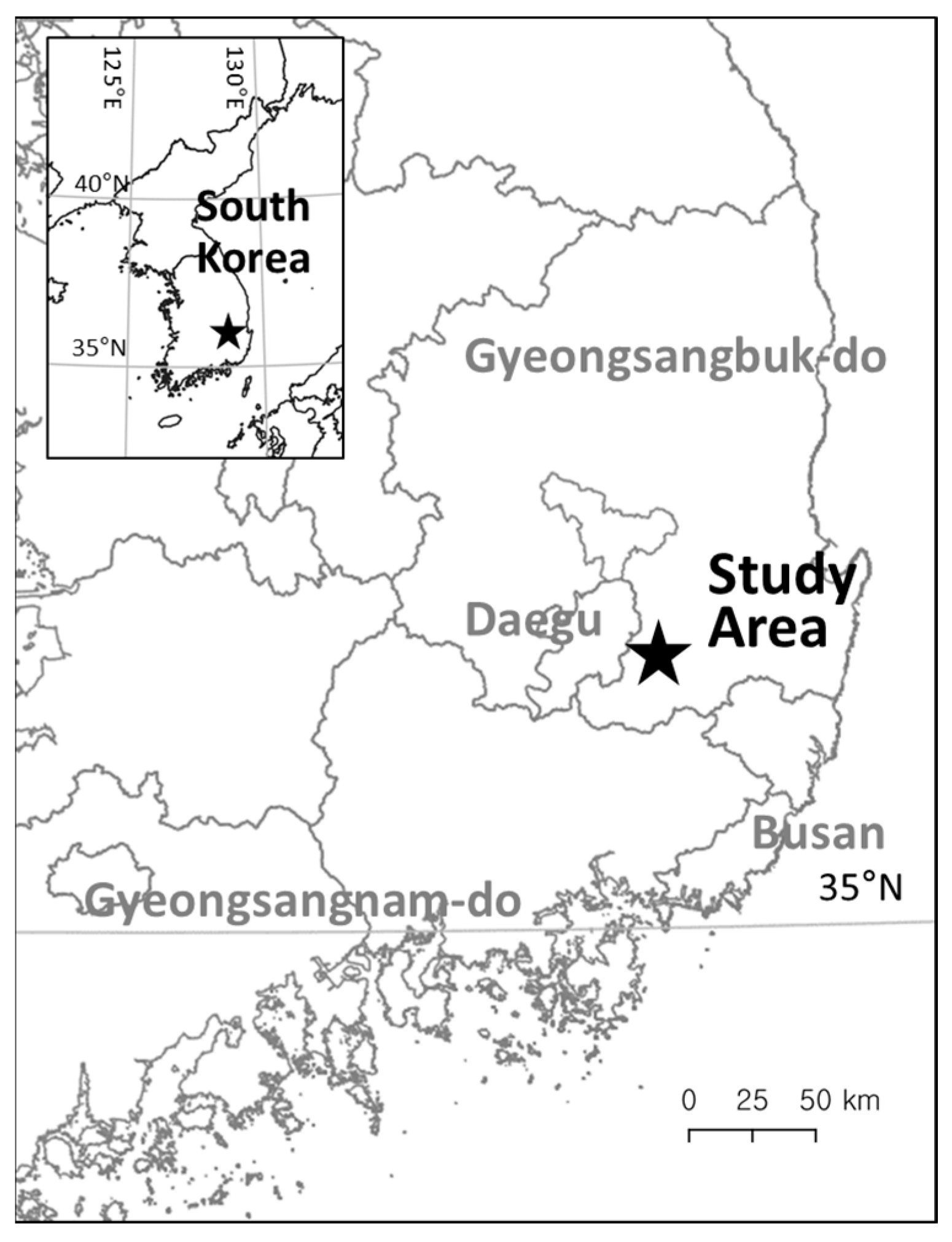
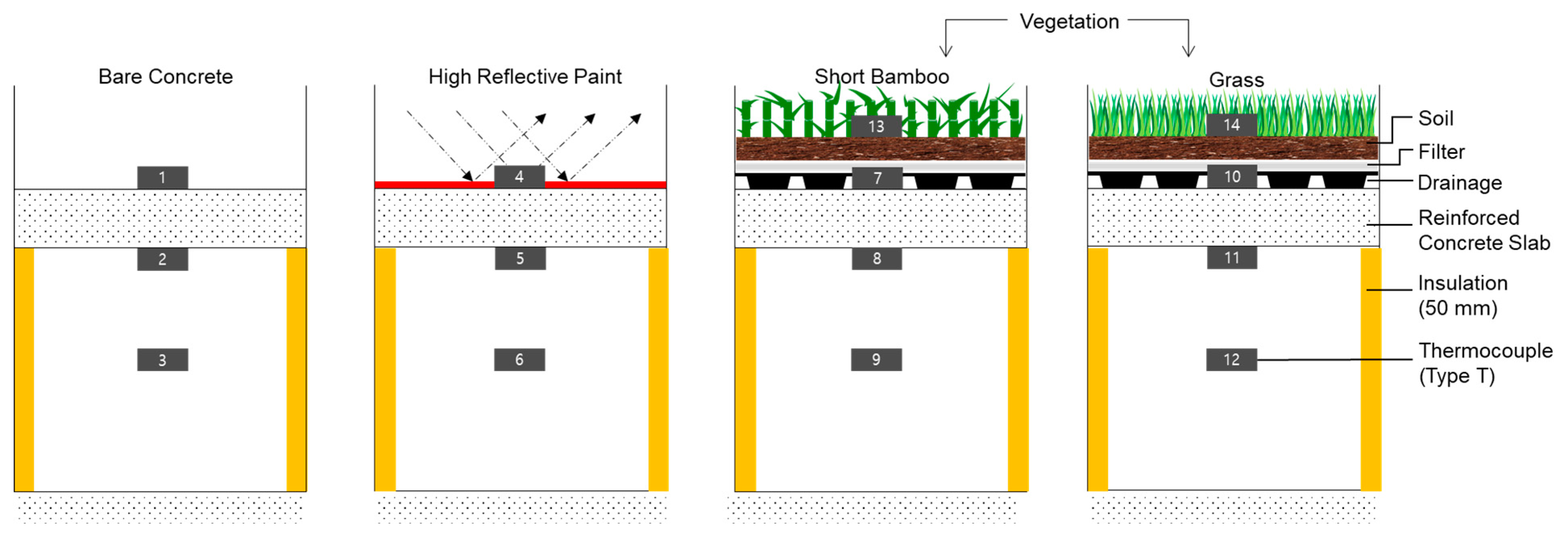
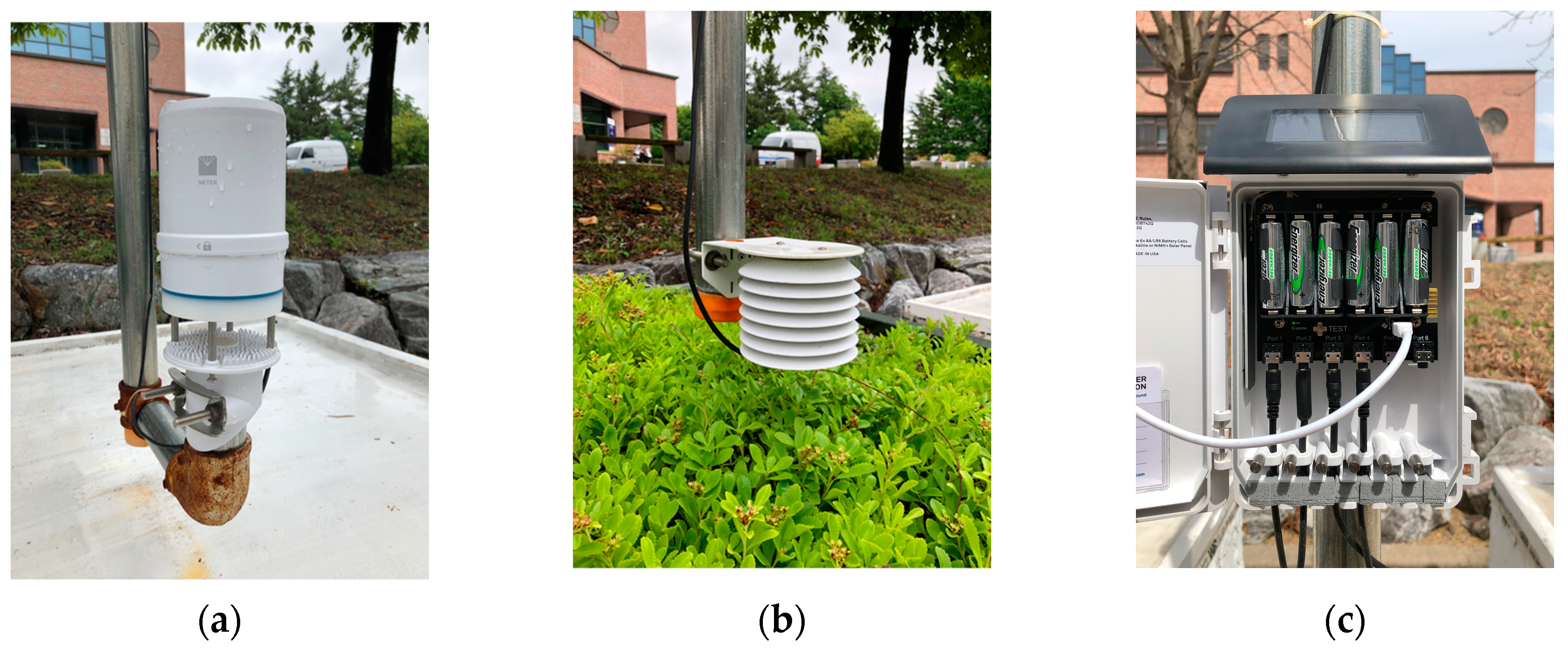
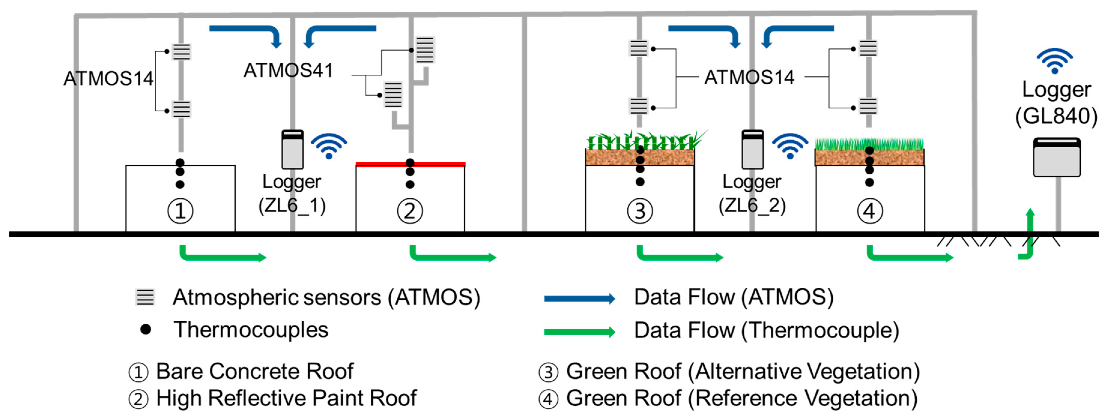
2.1. Study Area and Experimental Setup

In this study, four individual and separated experimental buildings were constructed. Temperatures, pressures, and wind speeds at two vertical points with different elevations were measured to estimate the surface energy balance for each roof type with the profile method.

The experiment site is located in Gyeonsan-si (city), Gyeongsangbuk-do (province), South Korea as shown in Figure 1. Gyeongsan, located in the southeastern region of South Korea (latitude: 35°49′23.99′′ N; longitude: 128°44′16.01′′ E), has a humid subtropical climate (Cfa) characterized by four distinct seasons. Summers, from June to August, are hot and humid, with average temperatures ranging from 25 °C to 35 °C (77 °F to 95 °F) and frequent monsoonal rains during the jangma season, contributing significantly to the annual rainfall of 1000 to 1500 mm (39 to 59 inches). Winters, from December to February, are relatively mild compared to northern regions, with temperatures averaging between −5 °C and 5 °C (23 °F to 41 °F), and with light snowfall occurring occasionally. Spring and autumn offer pleasant and comfortable weather, with average temperatures ranging from 15 °C to 25 °C (59 °F to 77 °F) and abundant sunshine. While Gyeongsan generally enjoys moderate weather, it occasionally experiences typhoons in late summer and early autumn, bringing heavy rainfall and strong winds. These climatic conditions make Gyeongsan favorable for agriculture and outdoor activities, particularly during the spring and autumn.

Figure 2 shows the four individual experiment buildings with different roof types, which were constructed close to the building of the Department of Civil Engineering in Yeungnam University’s Gyeongsan campus. The measurement process began in July, 2020, and the data for this study were collected during the mid-summer period from the 19th to the 26th of August, with a five-minute interval. Figure 3 illustrates the vertical roof structures of the experiment buildings. Figure 3 also shows the placement of the thermocouples used to capture temperature variations. The heights of the four buildings are basically the same (1.0 m). The widths and depths are also the same for all four buildings (1.1 m and 1.6 m, respectively). The thickness of the concrete roof is 0.09 m, with foam insulation (50 mm thickness) applied to the structure’s sidewalls to minimize the thermal influences from the outside atmosphere.

Roof surface temperatures can be measured using infrared (IR) thermometers, thermal imagers, or contact thermometers. The IR thermometers can provide a temperature reading quickly without any contact but are not as accurate as contact measurements. Contact thermometers are classified based on the sensor type used for the measurement, i.e., a thermocouple, resistance temperature detector (RTD), or thermistor. Selecting the proper sensor type is the first important step and mainly depends on the application and additional factors, like size, cost and accuracy. Most applications have a well-defined measurement range, accuracy requirement, and physical size constraints. Thermocouples are the most widely used sensors because of their low cost and wide temperature range. This study adopted the T-type thermocouple to measure temperature, considering application and maintenance.

As shown in Figure 3, building No. 1 (building 1) has a concrete roof, serving as the reference for other roof types. Building No. 2 (building 2) has a highly reflective painted roof, coated with a highly reflective paint (United Coatings Roof Mate Top Coat) to augment the roof’s reflectance, where the solar reflectance is suggested as 0.83 initially and 0.71 for the weathered condition. Buildings 3 and 4 have green roofs with two different types of vegetation—short bamboo and grass, respectively. Each green roof includes an additional 20 cm-deep soil layer, along with filter and drainage layers, categorizing them as extensive-type green roofs, as shown in Figure 3.

Figure 3 also shows the locations of the thermocouples, which were used to monitor temperatures of the buildings, including the roof, ceiling, and indoor temperatures. The concrete-roof building (building 1) has three thermocouples placed on the roof, ceiling, and indoors, which is the same as for the highly reflective painted-roof building (building 2). The green-roof buildings (buildings 3 and 4) have four thermocouples; three thermocouples are in the same places as in the other buildings, with one additional thermocouple on top of the soil. Before the installation of the green roofs and highly reflective paint, the temperatures from four buildings were compared, and the result showed the same thermal behavior inside and outside of the buildings. The temperature was crosschecked with other methodologies, such as IR thermometers and thermal images, and the results showed a good agreement with each other.

Figure 4 illustrates the atmospheric sensors used for this study. Figure 4a shows the METER ATMOS41 used to monitor temperature, humidity, atmospheric pressure, precipitation, wind speed, wind direction, and solar radiation at two vertical points on building 2. Figure 4b depicts the METER ATMOS14 used to measure temperature, humidity and atmospheric pressure at two vertical points for buildings 1, 3, and 4. Additionally, Figure 4c shows the ZL6 datalogger used to collect data from the ATMOS41 and ATMOS14 sensors.

Figure 5 illustrates the data collection schematic, including the datalogger and sensors. As previously mentioned, atmospheric data are collected using Meter’s ATMOS14 for buildings 1, 3, and 4 or ATMOS41 for building 2. Data from ATMOS14 for building 1 and ATMOS41 for building 2 were stored every five minutes by Meter’s ZL6 datalogger (Pullman, WA, USA). Similarly, data from the ATMOS14 sensors for buildings 3 and 4 were collected every five minutes by another ZL6 logger, as shown in Figure 5. The ZL6 logger is powered by a built-in photovoltaic cell, and the data can be accessed through a cloud service or via direct connection to the logger. Additionally, Figure 5 depicts the thermocouples used to measure building temperatures, including the roof, ceiling, and indoor temperatures, marked as black dots. The temperature data from the thermocouples were recorded every minute by Graphtec’s GL840-WV datalogger (YoKohama, Japan).

2.2. Net Radiation and Flux Profile Method

The net radiation (R_n) is obtained by considering the incoming radiation and outgoing radiation, which is given as the following equation. For clarity, it is helpful to distinguish shortwave radiation and longwave radiation, as follows [28]:

$$R_{n=}{F}_{SW}^{\downarrow }-F_{SW}^{\uparrow }+F_{LW}^{\downarrow }-F_{LW}^{\uparrow }$$

(1)

where R_n is the net radiation (W/m²). $F_{SW}^{\downarrow }$ is downwelling shortwave solar radiation (W/m²) transmitted through air. $F_{SW}^{\uparrow }$ is the reflected upwelling shortwave solar radiation (W/m²). Equation (1) can be rewritten using the shortwave albedo (A_SW) and the longwave albedo (A_LW) as follows:

$$R_n={(1-A_{SW})F}_{SW}^{\downarrow }+(1-A_{LW})F_{LW}^{\downarrow }$$

(2)

where $F_{LW}^{\downarrow }$ is longwave radiation (W/m²) downwards from the atmosphere. $F_{LW}^{\uparrow }$ is upward longwave radiation (W/m²). When further simplifying the above equation by neglecting the longwave term, considering incoming and outgoing longwave radiation cancel each other out, the equation becomes as follows:

$$R_{n }{=(1-A_{SW})F}_{SW}^{\downarrow }$$

(3)

In the meantime, the net radiation that reaches at the roof surface can be divided into four components, as follows:

$$R_n=L_E+H+G+\mathsf{\Delta }G$$

(4)

where L_E is the latent heat flux (W/m²), which is a portion of the net radiation used for the phase change of water. The latent heat flux is obtained by multiplying the evaporative flux E and the latent heat of vaporization ν. H is the sensible heat flux (W/m²), which is an energy flux portion that increases the surrounding temperatures. G is the ground heat flux (W/m²) that is transmitted into the building and contributes to increasing the indoor temperature. $\Delta$G is the amount of energy stored in the soil layer, which was ignored in this study.

The dynamic sublayer (10⁰ to 10¹ m from the surface) is a fully turbulent region near the ground surface, where the effects of the buoyancy force due to density stratification can be ignored. At the same time, the distance from the surface is enough that the viscosity of air and the structures of individual roughness elements have no effect on the motion. In the dynamic sublayer, the mean wind speed, mean temperature, and mean specific humidity have logarithmic profiles. The vertical profile of wind is influenced by atmospheric stability. In the surface sublayer, which extends from the viscous sublayer to the order of 10¹ m above the ground, atmospheric stability becomes a critical factor. Moreover, the effect of buoyancy becomes effective due to the vertical density gradient. To account for this, Monin and Obukhov introduced a rigorous theoretical indicator, ζ, known as the stability length scale, to characterize atmospheric stability [34,35,36,37]. Equations (5) and (6) are as follows:

$$\mathsf{\zeta }={\displaystyle \frac{z-z_0}{L}}$$

(5)

$$L={\displaystyle \frac{-{ u}_{*}^3 \rho }{kg[\frac{H}{T_a{c}_P}+0.61E]}}$$

(6)

where $\rho$ denotes the density of water, $c_p$ represents the specific heat capacity of water at a constant pressure (J/kg K), k is the von Karman constant, E is evaporation rate, and g is the gravitational acceleration (m/s²). The stability length is positive for stable, negative for unstable, and infinitely large for neutral conditions. z represents the height above the roof surface, while z₀ is the zero-plane displacement height depending on the rooftop roughness.

This study measured wind speed, temperature, and humidity at two different elevations, which was used to calculate the friction velocity, evaporation rate, and sensible heat flux using the following equations [23]:

$${\overline{u}}_2-{\overline{u}}_1={\displaystyle \frac{u_{*}}{k}}[ \ln \left({\displaystyle \frac{{\zeta }_2}{{\zeta }_1}}\right)-{\psi }_m({\zeta }_2)+{\psi }_m\left({\zeta }_1\right)]$$

(7)

$${\overline{q}}_1-{\overline{q}}_2={\displaystyle \frac{E}{k{u}_{*}\rho }}[ \ln \left({\displaystyle \frac{{\zeta }_2}{{\zeta }_1}}\right)-{\psi }_q({\zeta }_2)+{\psi }_q\left({\zeta }_1\right)]$$

(8)

$${\overline{\theta }}_1-{\overline{\theta }}_2={\displaystyle \frac{H}{k{u}_{*}\rho c_p}}[ \ln \left({\displaystyle \frac{{\zeta }_2}{{\zeta }_1}}\right)-{\psi }_h({\zeta }_2)+{\psi }_h\left({\zeta }_1\right)]$$

(9)

where q denotes the specific humidity. $\theta$ indicates the potential temperature. $u_{*}$ represents the friction velocity ($\mathrm{m}/\mathrm{s}$). ${\psi }_m$, ${\psi }_h$, and ${\psi }_q$ are the profile functions for stability correction. The number 1 represents the lower measurement point, which is near the surface, while the number 2 represents the other point, which is far from the surface. The functions are as follows [23]:

$${\psi }_m=2\mathit{ln}\left[{\displaystyle \frac{1+x}{2}}\right]+2\ln \left[{\displaystyle \frac{1+x^2}{2}}\right]-2{\mathit{tan}}^{-1}x+{\displaystyle \frac{\pi }{2}}$$

(10)

$${\psi }_h=2\ln \left[{\displaystyle \frac{1+x^2}{2}}\right]$$

(11)

$${\psi }_q=2\ln \left[{\displaystyle \frac{1+x^2}{2}}\right]$$

(12)

where x is equal to ${(1-16\zeta )}^{1/4}$.

The calculation starts with an assumption that L is infinitely long, which sets the entire profile function values to zero from Equations (10)–(12). This provides the initial estimates for E, H, and u*. Using these initial values, the profile functions are calculated, and E, H, u*, and L are iteratively recalculated until they converge, yielding the final estimation.

The ground heat flux represents the energy transmitted through roof material into the building interior. It depends on the temperature difference between the roof and the inside of the building. Equation (13) is as follows:

$$Q_G={-K}_s{\displaystyle \frac{(T_0-T_1)}{dz}}$$

(13)

where $K_s$ represents the conductivity of concrete (W/m K). $T_0$ denotes the temperature of the roof surface (upper surface of the concrete) (°C) and $T_1$ denotes the temperature of the indoor ceiling (°C). dz is the distance from the roof surface to the ceiling inside of the building. The net radiation can be calculated by adding all three components together, namely the sensible heat flux (Equation (9)), latent heat flux (Equation (8)), and ground heat flux (Equation (13)). The calculated net radiation values were then compared with and validated against the observed values obtained by Equation (3).

3. Results

This study examined the components of net radiation for different roof types, including concrete roofs, highly reflective painted roofs, and green roofs, using measurement data collected over one week, from the 19th of August at 00:00 to the 26th of August at 00:00, with a five-minute interval. The flux profile method requires wind speed and atmospheric pressure at two different elevations, along with temperature and humidity. Shear velocity, as defined in Equation (5), was determined using wind speed data from the two points. Specific humidity was calculated based on temperature, relative humidity, and atmospheric pressure measurements at the two elevations. These values were then used to compute the evaporation rate (E), as described in Equation (6). The study utilized two types of atmospheric sensors (METER’s ATMOS41 and ATMOS14), with the ATMOS41 being capable of measuring wind speed. As depicted in Figure 5, two ATMOS41 sensors were installed for building 2, and the wind speed data from building 2 were used for the flux calculations for all the other buildings.

3.1. Concrete Roof and Highly Reflective Painted Roof

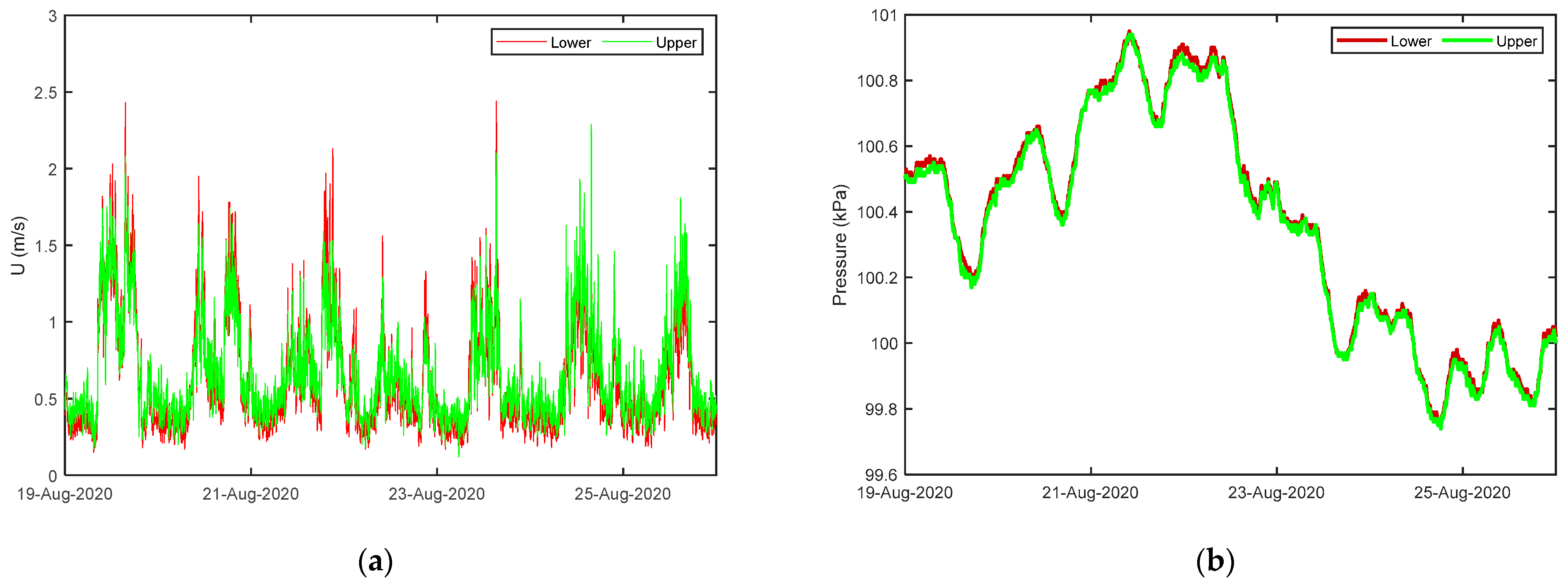
3.1.1. Wind Speed and Pressure Measurements

Figure 5 illustrates the wind speed and atmospheric pressure measured at two points using METER’s ATMOS41 (installed on building 2, the highly reflective painted roof) and ATMOS14 (installed on building 3, the green roof with short bamboo), respectively. The average wind speed during the measurement period (one week) was 0.6131 m/s at the lower point and 0.6635 m/s at the upper point, as shown in Figure 6a. Figure 6b presents the atmospheric pressure measured for building 3 at two points. The average atmospheric pressure during the study period was 100.369 kPa at the lower point and 100.355 kPa at the upper point.

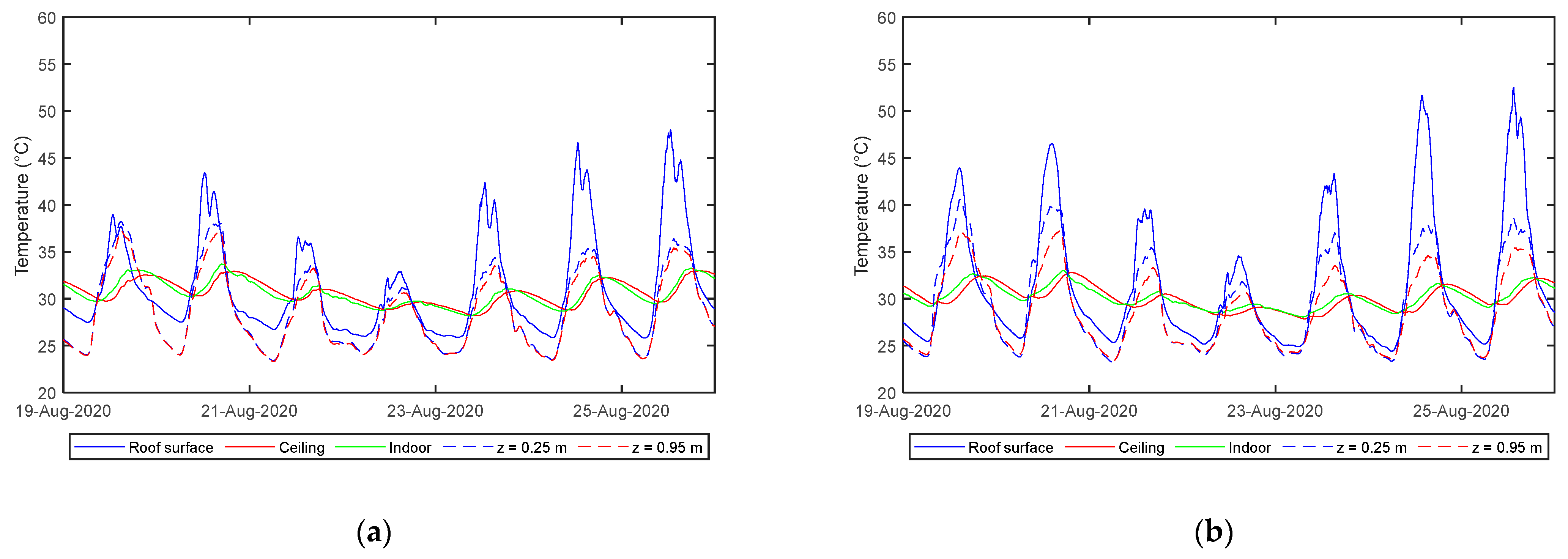
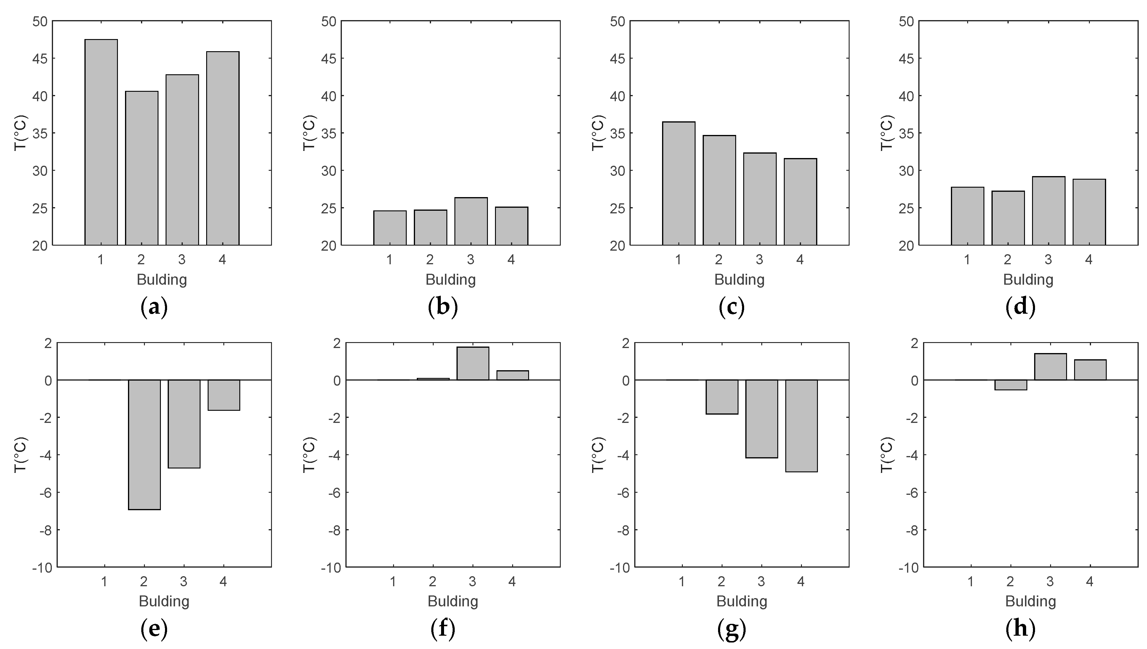
3.1.2. Temperature Measurements

Figure 7 illustrates the temporal variation in temperature at various locations, including the roof surface, ceiling, and indoor environment, as well as at two points above the roof surface. Temperatures at the roof surface, ceiling, and indoor environment were measured using T-type thermocouples, as detailed in the methodology section. The temperatures at the two points above the roof surface were recorded using atmospheric sensors (METER’s ATMOS14 for buildings 1, 3, and 4, and ATMOS41 for building 2). As shown in Figure 7a, the concrete roof exhibited higher surface temperatures during the daytime compared to the highly reflective painted roof, as seen in Figure 7. Notably, on August 19th and 20th, the surface temperature of the concrete roof exceeded 50 °C during the daytime, whereas the surface temperature of the highly reflective painted roof remained below 45 °C during the same period.

Table 1. Temperature measurements for the concrete-roof building and the highly reflective painted-roof building using thermocouples for roof surface, ceiling, and indoor measurements and ATMOS14 for two different points.

Temperature Sensor Location	Mean Temperature (°C)	Building
		Bare Concrete Roof (Building 1)	Highly Reflective Painted Roof (Building 2)
Roof surface	Total	32.74	30.87
	Daytime	37.33	33.96
	Nighttime	28.15	27.78
	Daily Maximum	47.50	40.57
	Daily Minimum	24.60	24.69
Ceiling	Total	32.02	30.38
	Daytime	34.62	31.97
	Nighttime	29.42	28.79
	Daily Maximum	42.21	37.20
	Daily Minimum	25.67	25.44
Indoor	Total	31.56	30.48
	Daytime	32.45	31.13
	Nighttime	30.68	29.83
	Daily Maximum	36.49	34.67
	Daily Minimum	27.75	27.22
Lower point above the roof surface	Total	29.54	28.77
	Daytime	32.28	30.83
	Nighttime	26.80	26.71
	Daily Maximum	37.55	34.98
	Daily Minimum	23.90	23.84
Upper point above the roof surface	Total	28.76	28.42
	Daytime	30.91	30.14
	Nighttime	26.61	26.70
	Daily Maximum	35.28	34.08
	Daily Minimum	23.77	23.82

presents the mean temperatures recorded at various measurement locations for both the concrete roof and the highly reflective painted roof. The concrete roof consistently exhibited higher overall mean temperatures, daytime averages, and daily maximum mean temperatures compared to the highly reflective painted roof across all measurement points. Notably, the daily maximum mean temperature at the surface of the concrete roof reached 47.50 °C, which was 6.93 °C higher than the corresponding value for the highly reflective painted roof (40.57 °C). The indoor temperature of the highly reflective painted-roof building was also lower than for the concrete-roof building. The daily maximum indoor mean temperature was 34.67 °C, which was lower by 1.80 °C compared to the concrete-roof building. The temperature measurements of the lower and upper point above the roof surface showed the diurnal variation in the vertical temperature profile. During the daytime, the surface temperature rises as the surface absorbs the solar radiation, and then the temperature propagates upward to the air, so the temperature decreases as the altitude increases. However, these profiles invert during the nighttime, when the surface temperature drops faster than the air temperature.

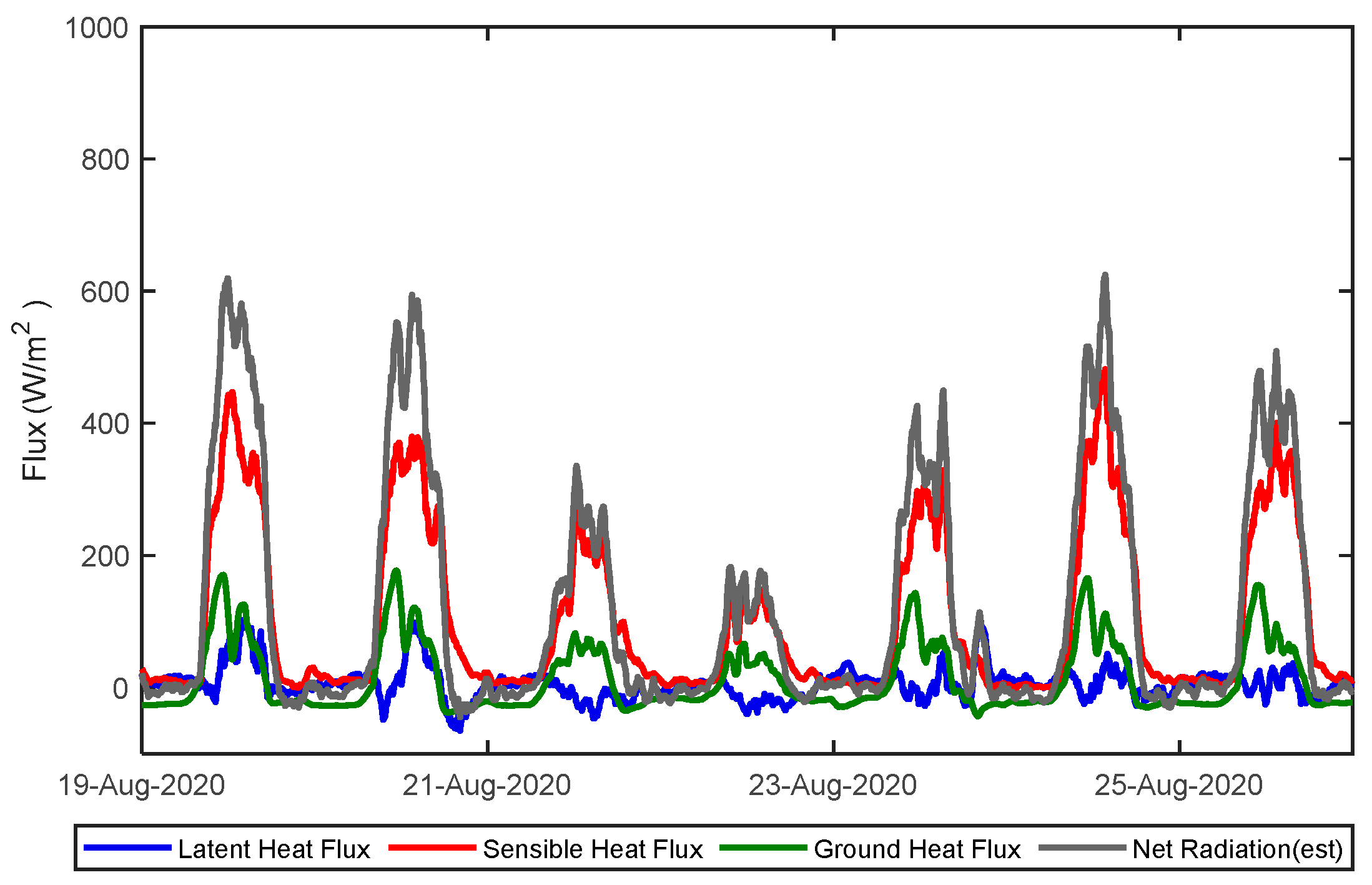
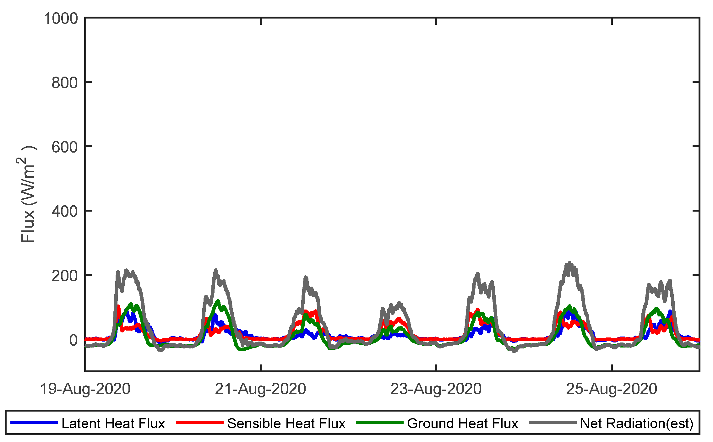
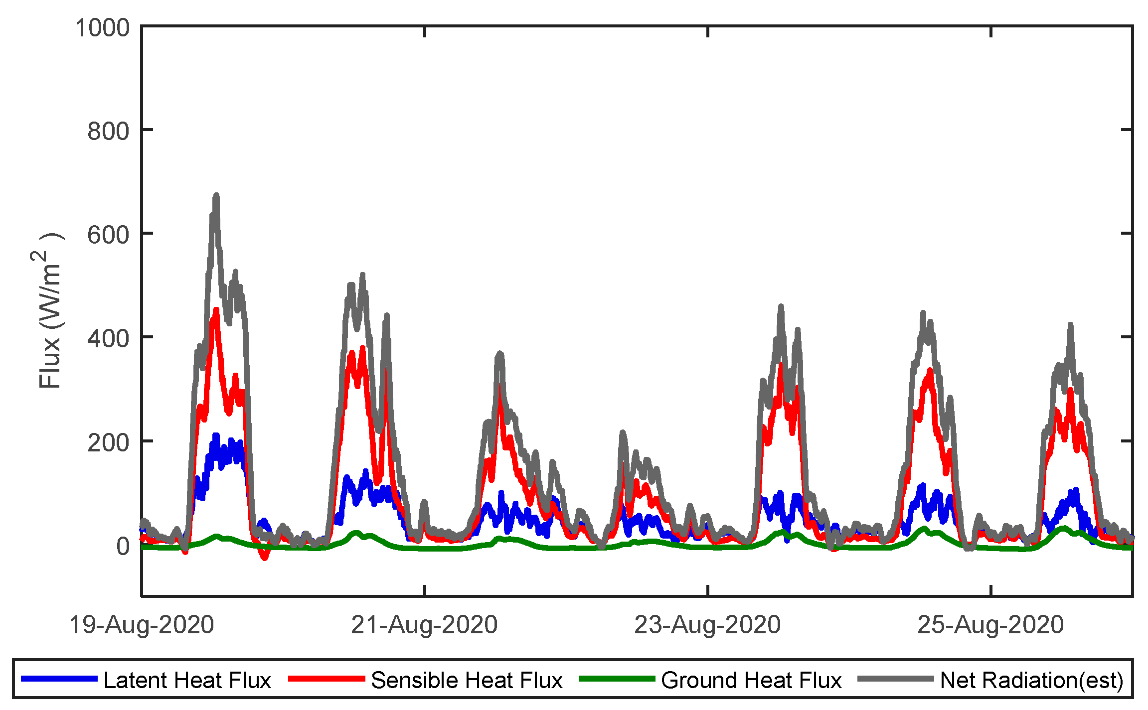
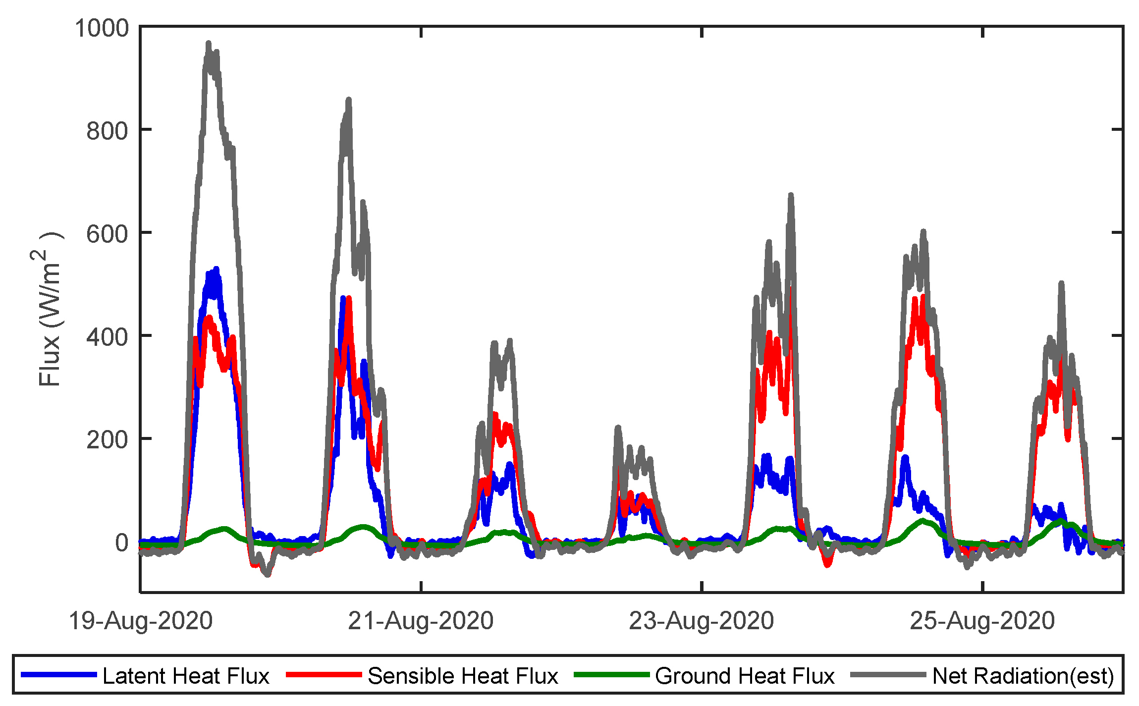
3.1.3. Estimation of Surface Energy Balance

Equations (1) and (2) shows the surface energy balance equation, where the net radiation is the sum of sensible heat flux, latent heat flux, and ground heat flux, assuming that the energy storage (ΔG) is negligible. Figure 8 and Figure 9 show the estimated net radiation for the concrete-roof building and the highly reflective painted-roof building, respectively, using the flux profile method. The sensible heat flux and latent heat flux were calculated from the observed wind speed, atmospheric pressure, and temperature at two different points, as described earlier in the methodology section. The ground heat flux was also calculated using the temperature measurements at two different points (the roof surface and ceiling). The results showed that the mean net radiation during the experiment period was 123.18 W/m² for the concrete-roof building, whereas it was 42.99 W/m² for the highly reflective painted-roof building due to the high albedo of the painted roof.

3.2. Green Roofs

3.2.1. Temperature and Pressure Measurements

Figure 10 shows the temperature variation inside and outside of the green roofs during the experiment period for one week (August 19th to 26th). In general, the surface temperature and indoor temperatures were lower than with the concrete roof. In particular, the indoor temperature showed stable changes compared to the fluctuation of the concrete-roof building. The temperature showed similar behaviors for both green-roofed buildings. The total mean temperatures were 30.6 °C (short bamboo) and 30.13 °C (grass) regardless of the vegetation type (grass for building 4 and short bamboo for building 3). The surface temperatures of the short bamboo roof were higher than for the grass roof. The daytime mean temperature of the short bamboo roof was 35.38 °C and the maximum mean was 45.88 °C, which were higher than 1.1 °C and 3.09 °C compared to the grass roof, respectively. These results were caused by the vegetation type, because the short bamboo did not cover the entire soil surface compared to grass, which resulted in a lower albedo as more net radiation reached the surface.

Table 2. Temperature measurements for green-roof building 1 (grass) and green-roof building 2 (short bamboo) using thermocouples for roof surface, ceiling, and indoor measurements and ATMOS14 for two different points.

Temperature Sensor Location	Mean Temperature (°C)	Building
		Green Roof (Grass) (Building 4)	Green Roof (Short Bamboo) (Building 3)
Roof surface	Total	31.23	31.52
	Daytime	34.28	35.38
	Nighttime	28.19	27.65
	Daily Maximum	42.79	45.88
	Daily Minimum	26.36	25.09
Ceiling	Total	30.64	30.05
	Daytime	30.09	29.53
	Nighttime	31.19	30.57
	Daily Maximum	32.10	31.59
	Daily Minimum	29.29	28.87
Indoor	Total	30.60	30.13
	Daytime	30.29	30.01
	Nighttime	30.91	30.24
	Daily Maximum	32.33	31.58
	Daily Minimum	29.16	28.83
Lower point above the roof surface	Total	28.96	29.54
	Daytime	31.32	32.62
	Nighttime	26.61	26.46
	Daily Maximum	35.81	37.97
	Daily Minimum	23.77	23.61
Upper point above the roof surface	Total	28.58	28.67
	Daytime	30.65	30.71
	Nighttime	26.50	26.63
	Daily Maximum	34.82	34.88
	Daily Minimum	23.70	23.80

lists the mean temperatures recorded at various measurement locations for both green roofs. Green roofs showed distinctively different results compared to the concrete roof or the highly reflective painted-roof buildings across all ceiling and indoor measurement points. Notably, the daily maximum mean indoor temperatures were 32.33 °C and 31.58 °C for the grass roof and the short bamboo roof, respectively. These results were lower than the concrete roof by 4.16 °C and 4.91 °C for each building. Figure 11a shows that the surface temperatures of the green roofs were lower than the concrete roof but higher than the highly reflective painted roof. However, these higher temperatures do not contribute to the indoor temperature increases, as shown in Figure 11c,g, due to the insulation effects from the substrates of the green roofs. Figure 11f,h also shows that the minimum mean temperature of the concrete roof was lower than green roofs.

3.2.2. Estimation of Surface Energy Balance

Figure 12 and Figure 13 illustrate the estimated net radiation for the green-roof buildings (obtained from the flux profile method). The results showed that the mean net radiation during the experiment period was 136.99 W/m² for the grass-roof building, whereas it was 149.48 W/m² for the short bamboo-roof building due to the lower albedo of the short bamboo roof. Particularly, the green roofs showed higher portions of the latent heat flux compared to the previous roof types, such as the concrete roof and highly reflective painted roof. The latent heat fluxes were 91.54 W/m² and 93.58 W/m² for the grass and short bamboo roofs, respectively, compared to the concrete roof (5.73 W/m²) and the highly reflective painted roof (14.58 W/m²). The ratios of the latent heat fluxes were also higher than roofs without vegetation, as shown in

Table 3. Estimated net radiation (R_n) and fluxes using the flux profile method. The percentage values inside the brackets show the ratio of each flux compared to the net radiation.

Building	Rn	QH	QE	QG
Bare concrete roof	123.18	103.81 (84%)	5.73 (5%)	13.63 (11%)
Highly reflective painted roof	42.99	19.40 (45%)	14.35 (33%)	9.23 (22%)
Grass roof	136.99	91.54 (67%)	44.38 (32%)	1.05 (1%)
Short bamboo roof	149.48	93.58 (63%)	53.28 (36%)	2.61 (1%)

.

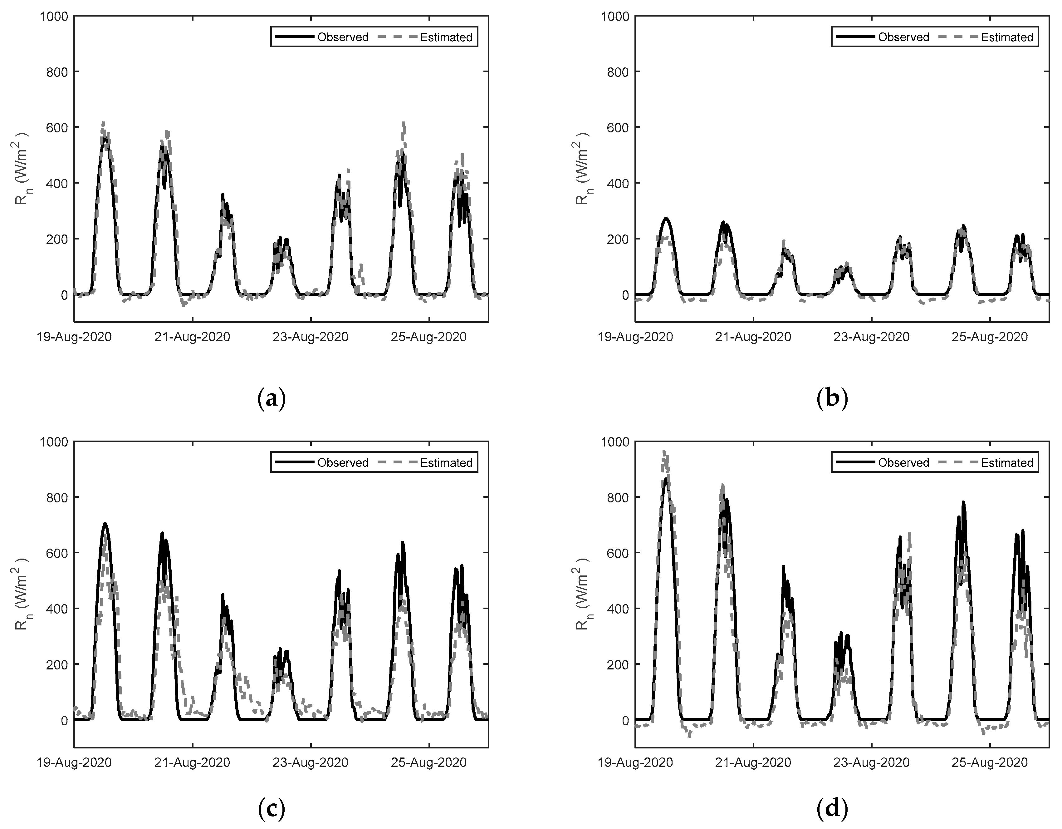
3.3. Comparison with the Observed Net Radiation

Figure 14 shows the estimated net radiation results, which represent the sum of the sensible heat flux, latent heat flux, and ground heat flux as given in Equation (2), compared with the observed net radiation from ATMOS41. In general, the results demonstrate the robustness of the flux profile method in estimating each energy flux and net radiation, with the Nash–Sutcliffe efficiency (NE) used to evaluate the estimation’s performance. The NE was highest for the concrete roof (Figure 14a), at 0.9297, and lowest for the grass roof, at 0.7950. The NE values were 0.8955 for the highly reflective painted roof and 0.8915 for the short bamboo roof. It should be noted that the observed net radiation is limited to shortwave radiation due to the sensor’s inability to monitor longwave radiation. However, longwave radiation can be neglected because the incoming and outgoing components of longwave radiation balance each other out. In this regard, the estimation of the albedo is important to calculate the observed net radiation as given in Equation (1). This topic will be discussed in detail in the Discussion section.

4. Discussion

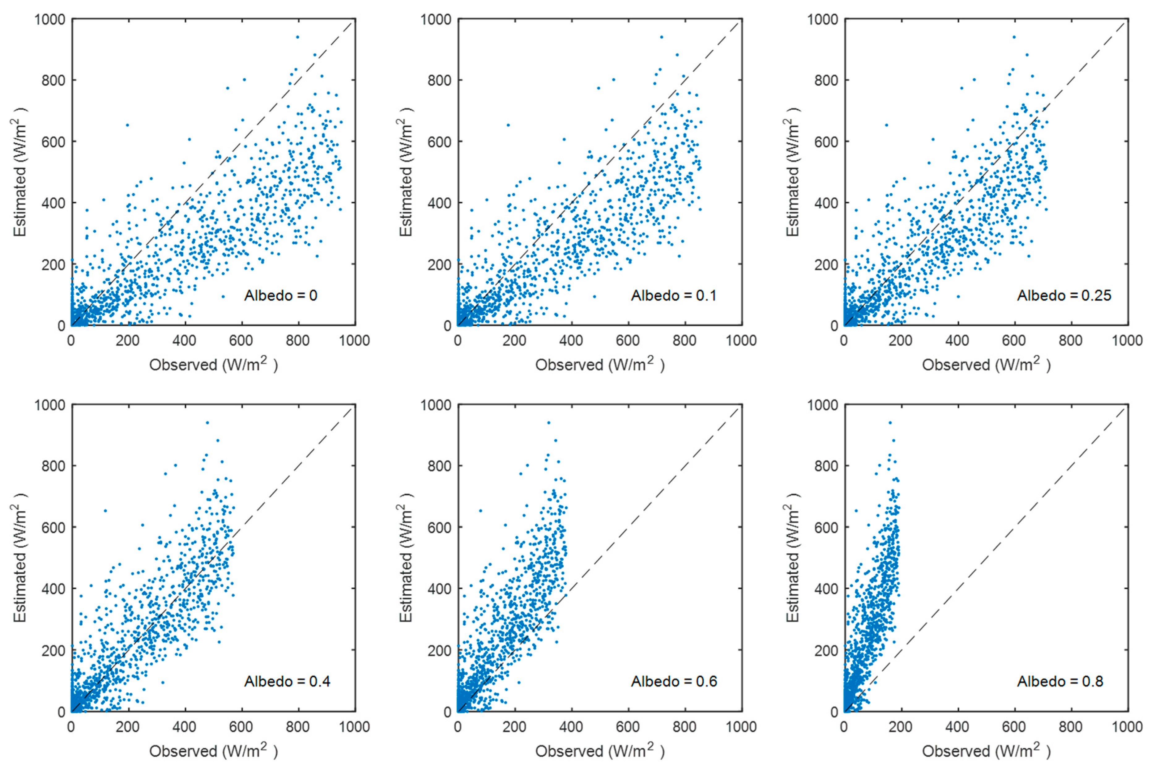
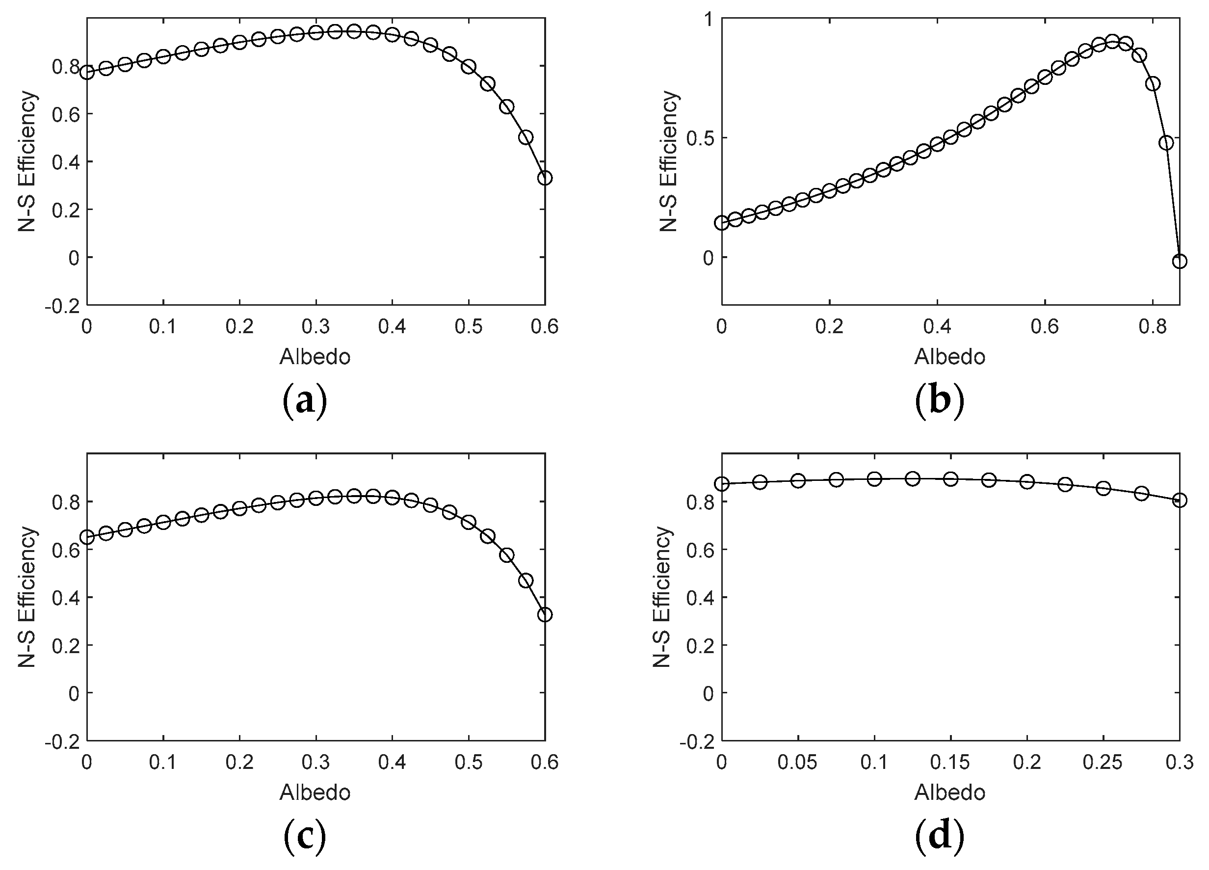
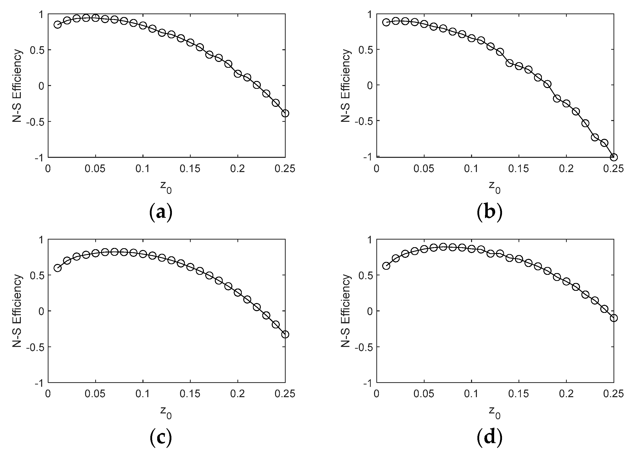
Sensitivity Analysis of the Albedo

The albedo plays a crucial role in determining the observed net radiation. Figure 15 compares the observed net radiation with the estimated value from the flux profile method, highlighting the significant influence of albedo on the method’s accuracy and alignment with observations. To further explore this relationship, Figure 16 presents a sensitivity analysis of the albedo for each roof type. The results showed that each roof has an optimal and original albedo value that closely matches the observed data.

Figure 16a shows that the optimal albedo value for the concrete roof is 0.35, which falls within the expected physical range for concrete surfaces. Similarly, Figure 16b shows that the highly reflective painted roof has an optimal albedo of 0.70, aligning closely with the product specifications (Roof Mate Top Coat: 0.83 initially and 0.71 in weathered conditions). For the grass roof, Figure 16c identifies an optimal albedo value of 0.375. Figure 16d reveals that the optimal albedo value for the short bamboo roof is 0.125, which is lower than that of the grass roof, despite both being green roofs.

Another important parameter is roughness height (z₀), using the flux profile method as proposed in Equation (3) for the stability length. Figure 17 shows the sensitivity analysis of the roughness height for each roof. The results also show appropriate optimum values for each roof types considering the physical properties of roughness. Figure 17a,b show that the optimum values for the roughness height are 0.05 and 0.0125 for the concrete roof and highly reflective roof, respectively. Theoretically, the roughness height of these two types should be 0 because there is no vegetation and no obstacles. However, each roof has a 5 cm height boundary wall for construction purposes and this can cause higher optimum values. Figure 17c,d show that the optimum values for the roughness height are 0.07 for both green roofs. Both green roofs showed higher optimum roughness values compared to the concrete-surfaced roofs.

5. Conclusions

This study introduced the flux profile method as a straightforward and practical approach to estimate the surface energy balance of green roofs, offering a cost-effective alternative to expensive monitoring systems by relying on basic measurements at two points. To prevent any temperature disturbances, four independent and insulated experimental buildings were constructed, each with a distinct roof type: concrete, highly reflective paint, short bamboo, and grass. The flux profile method was employed to estimate sensible and latent heat fluxes using temperature, atmospheric pressure, and wind speed measurements taken at two different heights, demonstrating its practicality and applicability. The results showed the net radiation estimated by the flux profile method coincided with the observed data. The findings validated the method’s reliability in estimating heat fluxes across all roof types. Additionally, sensitivity analysis revealed that the optimal values of albedo and surface roughness for each roof type fell within reasonable physical ranges, further supporting the method’s credibility. The results also highlighted that a green roof significantly reduced the sensible heat flux by increasing the proportion of the latent heat flux. The grass roof reduced the absolute amount of sensible heat flux by 11.8% compared to the concrete roof. The surface energy balance analysis of the green roofs suggests that this methodology could be a valuable tool for quantitatively assessing the benefits of green roofs, particularly in mitigating urban heat islands and reducing building energy consumption. These results can be affected by local experimental conditions, such as local climate conditions, soil and vegetation conditions, and so forth, because the methodology depends on the vertical profiles of temperature and humidity. However, the contribution of the vegetation (green roof) to increasing the portion of the latent heat flux is expected to remain valid in different regions.

References

1. Slaney, S. Stormwater Management for Sustainable Urban Environments; Images Publishing Group Pty Limited: Chadstone, VIC, Australia, 2016. [Google Scholar]
2. Ascione, F.; Bianco, N.; de’ Rossi, F.; Turni, G.; Vanoli, G.P. Green roofs in European climates. Are effective solutions for the energy savings in air-conditioning? Appl. Energy 2013, 104, 845–859. [Google Scholar] [CrossRef]
3. Ávila-Hernández, A.; Simá, E.; Xamán, J.; Hernández-Pérez, I.; Téllez-Velázquez, E.; Chagolla-Aranda, M.A. Test box experiment and simulations of a green-roof: Thermal and energy performance of a residential building standard for Mexico. Energy Build. 2020, 209, 109709. [Google Scholar] [CrossRef]
4. Baraldi, R.; Neri, L.; Costa, F.; Facini, O.; Rapparini, F.; Carriero, G. Ecophysiological and micromorphological characterization of green roof vegetation for urban mitigation. Urban For. Urban Green. 2019, 37, 24–32. [Google Scholar] [CrossRef]
5. Brutsaert, W. Evaporation into the Atmosphere: Theory, History, and Applications; Springer: Dordrecht, The Netherlands, 1982; 299p. [Google Scholar]
6. Businger, J.A.; Yaglom, A.M. Introduction to Obukhov’s paper on ‘turbulence in an atmosphere with a non-uniform temperature’. Bound.-Layer Meteorol. 1971, 2, 3–6. [Google Scholar] [CrossRef]
7. Cai, L.; Feng, X.-P.; Yu, J.-Y.; Xiang, Q.-C.; Chen, R. Reduction in Carbon Dioxide Emission and Energy Savings Obtained by Using a Green Roof. Aerosol Air Qual. Res. 2019, 19, 2432–2445. [Google Scholar] [CrossRef]
8. Castiglia Feitosa, R.; Wilkinson, S. Modelling green roof stormwater response for different soil depths. Landsc. Urban Plan. 2016, 153, 170–179. [Google Scholar] [CrossRef]
9. Collins, S.; Kuoppamäki, K.; Kotze, D.J.; Lü, X. Thermal behavior of green roofs under Nordic winter conditions. Build. Environ. 2017, 122, 206–214. [Google Scholar] [CrossRef]
10. Costa-Filho, E.; Chávez, J.L.; Zhang, H.; Andales, A.A. An optimized surface aerodynamic temperature approach to estimate maize sensible heat flux and evapotranspiration. Agric. For. Meteorol. 2021, 311, 108683. [Google Scholar] [CrossRef]
11. Gregoire, B.G.; Clausen, J.C. Effect of a modular extensive green roof on stormwater runoff and water quality. Ecol. Eng. 2011, 37, 963–969. [Google Scholar] [CrossRef]
12. Hathaway, M.A.; Hunt, F.W.; Jennings, D.G. A Field Study of Green Roof Hydrologic and Water Quality Performance. Trans. ASABE 2008, 51, 37–44. [Google Scholar] [CrossRef]
13. Heusinger, J.; Weber, S. Surface energy balance of an extensive green roof as quantified by full year eddy-covariance measurements. Sci. Total Environ. 2017, 577, 220–230. [Google Scholar] [CrossRef]
14. Kotsiris, G.; Androutsopoulos, A.; Polychroni, E.; Souliotis, M.; Kavga, A. Carbon footprint of green roof installation on school buildings in Greek Mediterranean climatic region. Int. J. Sustain. Energy 2019, 38, 866–883. [Google Scholar] [CrossRef]
15. Li, Y.; Babcock, R.W. Green roofs against pollution and climate change. A review. Agron. Sustain. Dev. 2014, 34, 695–705. [Google Scholar] [CrossRef]
16. Lin, B.-S.; Yu, C.-C.; Su, A.-T.; Lin, Y.-J. Impact of climatic conditions on the thermal effectiveness of an extensive green roof. Build. Environ. 2013, 67, 26–33. [Google Scholar] [CrossRef]
17. Liu, K.; Bass, B. Performance of green roof systems. In Proceedings of the Cool Roofing Symposium, Toronto, ON, Canada, 12–13 May 2005; pp. 1–18. [Google Scholar]
18. Mehdi, R.; Nyirumuringa, E.; Juyeon, K.; Doo Hwan, K. Analyzing the Impact of Green Roof Functions on the Citizens’ Mental Health in Metropolitan Cities. Iran. J. Public Health 2021, 50, 900. [Google Scholar] [CrossRef]
19. Moghbel, M.; Erfanian Salim, R. Environmental benefits of green roofs on microclimate of Tehran with specific focus on air temperature, humidity and CO2 content. Urban Clim. 2017, 20, 46–58. [Google Scholar] [CrossRef]
20. Monin, A.S.; Obukhov, A.M. Basic laws of turbulent mixing in the surface layer of the atmosphere. Tr. Akad. Nauk SSSR Geophiz. Inst. 1954, 24, 163–187. [Google Scholar]
21. Peng, L.L.H.; Jim, C.Y. Economic evaluation of green-roof environmental benefits in the context of climate change: The case of Hong Kong. Urban For. Urban Green. 2015, 14, 554–561. [Google Scholar] [CrossRef]
22. Peng, Z.J.; Stovin, V. Independent Validation of the SWMM Green Roof Module. J. Hydrol. Eng. 2017, 22, 04017037. [Google Scholar] [CrossRef]
23. Prueger, J.H.; Kustas, W.P. Aerodynamic Methods for Estimating Turbulent Fluxes; Micrometeorology in Agricultural Systems Agricultural Research Service: Lincoln, NE, USA, 2005; pp. 407–436. [Google Scholar]
24. Qin, X.; Wu, X.; Chiew, Y.; Li, Y. A green roof test bed for stormwater management and reduction of urban heat island effect in Singapore. Br. J. Environ. Clim. Change 2013, 2, 410–420. [Google Scholar] [CrossRef]
25. Sailor, D.J. A green roof model for building energy simulation programs. Energy Build. 2008, 40, 1466–1478. [Google Scholar] [CrossRef]
26. Santamouris, M. Cooling the cities—A review of reflective and green roof mitigation technologies to fight heat island and improve comfort in urban environments. Sol. Energy 2014, 103, 682–703. [Google Scholar] [CrossRef]
27. Speak, A.F.; Rothwell, J.J.; Lindley, S.J.; Smith, C.L. Urban particulate pollution reduction by four species of green roof vegetation in a UK city. Atmos. Environ. 2012, 61, 283–293. [Google Scholar] [CrossRef]
28. Stull, R.B. An Introduction to Boundary Layer Meteorology; Kluwer Academic Publishers: Dordrecht, The Netherlands; Boston, MA, USA, 1988; 666p. [Google Scholar]
29. Fortuniak, K.; Pawlak, W.; Siedlecki, M. Integral Turbulence Statistics Over a Central European City Centre. Bound.-Layer Meteorol. 2013, 146, 257–276. [Google Scholar] [CrossRef]
30. Montgomery, R.B. Vertical Eddy Flux of Heat in the Atmosphere. J. Atmos. Sci. 1948, 5, 265–274. [Google Scholar] [CrossRef]
31. Swinbank, W.C. The Measurement of Vertical Transfer of Heat and Water Vapor by Eddies in the Lower Atmosphere. J. Atmos. Sci. 1951, 8, 135–145. [Google Scholar] [CrossRef]
32. Wyngaard, J.C.; Clifford, S.F. Estimating Momentum, Heat and Moisture Fluxes from Structure Parameters. J. Atmos. Sci. 1978, 35, 1204–1211. [Google Scholar] [CrossRef]
33. Gawuc, L.; Łobocki, L.; Strużewska, J. Application of the profile method for the estimation of urban sensible heat flux using roadside weather monitoring data and satellite imagery. Urban Clim. 2022, 42, 101098. [Google Scholar] [CrossRef]
34. USEPA. Green Roofs for Stormwater Runoff Control; EPA/600/R-09/026; United States Environmental Protection Agency: Washington, DC, USA, 2009. [Google Scholar]
35. Van der Meulen, S.H. Costs and Benefits of Green Roof Types for Cities and Building Owners. J. Sustain. Dev. Energy Water Environ. Syst. 2019, 7, 57–71. [Google Scholar] [CrossRef]
36. VanWoert, N.D.; Rowe, D.B.; Andresen, J.A.; Rugh, C.L.; Fernandez, R.T.; Xiao, L. Green Roof Stormwater Retention. J. Environ. Qual. 2005, 34, 1036–1044. [Google Scholar] [CrossRef]
37. William, R.; Goodwell, A.; Richardson, M.; Le, P.V.V.; Kumar, P.; Stillwell, A.S. An environmental cost-benefit analysis of alternative green roofing strategies. Ecol. Eng. 2016, 95, 1–9. [Google Scholar] [CrossRef]
Figure 1. Location map of the study area.
Sustainability 17 02725 g001
Figure 2. Experiment buildings (concrete boxes) for different types of roofs, including (a) bare concrete (No. 1), (b) highly reflective paint (No. 2), (c) short bamboo (No. 3), and (d) grass roof (No. 4).
Sustainability 17 02725 g002
Figure 3. Experiment buildings schematic which shows where the thermocouples (gray squares with numbers) are located in each building.
Sustainability 17 02725 g003
Figure 4. Atmospheric sensors: (a) METER ATMOS41 for monitoring temperature, humidity, atmospheric pressure, precipitation, wind speed, wind direction, and solar radiation at two different points; (b) METER ATMOS14 for temperature, humidity, and atmospheric pressure at two different points; (c) ZL6 datalogger.
Sustainability 17 02725 g004
Figure 5. Green roof monitoring system schematic.
Sustainability 17 02725 g005
Figure 6. Wind speed and atmospheric pressure at two points measured using METER’s ATMOS41 and ATMOS14: (a) wind speed using ATMOS41; (b) atmospheric pressure using ATMOS14 for the concrete-roof building.
Sustainability 17 02725 g006
Figure 7. Temperature measurements for (a) the concrete-roof building and (b) the highly reflective painted-roof building using thermocouples for roof surface, ceiling, and indoor measurements and ATMOS14 for two different points.
Sustainability 17 02725 g007
Figure 8. Estimated net radiation (Rn) of the concrete roof from the flux profile method; the net radiation was estimated by summing the latent heat flux, sensible heat flux, and ground heat flux.
Sustainability 17 02725 g008
Figure 9. Estimated net radiation (Rn) of the highly reflective painted roof from the flux profile method; the net radiation was estimated by summing the latent heat flux, sensible heat flux, and ground heat flux.
Sustainability 17 02725 g009
Figure 10. Temperature measurements for (a) green-roof building 1 (grass) and (b) green-roof building 2 (short bamboo) using thermocouples for roof surface, ceiling, and indoor measurements and ATMOS14 for two different points.
Sustainability 17 02725 g010
Figure 11. (a) Daily maximum mean temperatures at the roof surface; (b) daily minimum mean temperatures at the roof surface; (c) daily maximum indoor temperatures; (d) daily minimum indoor temperatures; the difference to the concrete roof for (e) daily maximum and (f) minimum at the roof surface; (g) daily maximum and (h) minimum indoor temperature differences.
Sustainability 17 02725 g011
Figure 12. Estimated net radiation (Rn) of the green roof (grass) from the flux profile method; the net radiation was estimated by summing the latent heat flux, sensible heat flux, and ground heat flux.
Sustainability 17 02725 g012
Figure 13. Estimated net radiation (Rn) of the green roof (short bamboo) from the flux profile method; the net radiation was estimated by summing the latent heat flux, sensible heat flux, and ground heat flux.
Sustainability 17 02725 g013
Figure 14. Comparison of the net radiation estimated from the flux profile method with the observed radiation for (a) the concrete roof (NE 0.9297); (b) the highly reflective painted roof (NE 0.8955); (c) green roof 1 (grass) (NE 0.7950); and (d) green roof 2 (short bamboo) (NE 0.8915).
Sustainability 17 02725 g014
Figure 15. Comparison of the observed and estimated net radiation for the concrete roof, which shows the sensitivity to the value of the albedo.
Sustainability 17 02725 g015
Figure 16. Sensitivity analysis to the value of the albedo: (a) the concrete roof; (b) the highly reflective painted roof; (c) the grass roof; (d) the short bamboo roof.
Sustainability 17 02725 g016
Figure 17. Sensitivity analysis to the value of the roughness height, z0: (a) the concrete roof; (b) the highly reflective painted roof; (c) the grass roof; (d) the short bamboo roof.
Sustainability 17 02725 g017