A Two-Layer Cooperative Optimization Approach for Coordinated Photovoltaic-Energy Storage System Sizing and Factory Energy Dispatch Under Industrial Load Profiles

Abstract

Driven by policy incentives and economic pressures, energy-intensive industries are increasingly focusing on energy cost reductions amid the rapid adoption of renewable energy. However, the existing studies often isolate photovoltaic-energy storage system (PV-ESS) configurations from detailed load scheduling, limiting industrial park energy management. To address this, we propose a two-layer cooperative optimization approach (TLCOA). The upper layer employs a genetic algorithm (GA) to optimize the PV capacity and energy storage sizing through natural selection and crossover operations, while the lower layer utilizes mixed integer linear programming (MILP) to derive cost-minimized scheduling strategies under time-of-use tariffs. Multi-process parallel computing accelerates the fitness evaluations, resolving high-dimensional industrial data challenges. Multi-process parallel computing is introduced to accelerate fitness evaluations, effectively addressing the challenges posed by high-dimensional industrial data. Validated with real power market data, the TLCOA demonstrated rapid adaptation to load fluctuations while achieving a 23.68% improvement in computational efficiency, 1.73% reduction in investment costs, 7.55% decrease in power purchase costs, and 8.79% enhancement in renewable energy utilization compared to traditional methods. This integrated framework enables cost-effective PV-ESS deployment and adaptive energy management in industrial facilities, offering actionable insights for renewable integration and scalable energy optimization.

1. Introduction

In response to the global warming challenge driven by high levels of carbon dioxide emissions, the international community has widely advocated for the adoption of clean energy and a reduction in carbon emissions to achieve sustainable economic and social development [1]. The industrial sector, including the power industry, is the largest source of carbon emissions in China. Identifying feasible and effective emission reduction strategies within this sector is crucial to achieving China’s carbon peak and carbon neutrality goals [2]. The increasing global energy demand and the transition towards sustainable energy solutions have driven the integration of renewable energy sources into industrial power systems. Industrial parks, as major energy consumers, face challenges in optimizing energy consumption while ensuring cost-effectiveness and sustainability.

Industrial parks, which consist of multiple industrial load facilities, are particularly suitable for integrating renewable energy systems such as photovoltaic-energy storage system (PV-ESS). PV-ESS refers to an integrated system of photovoltaic (PV) power generation and an energy storage system (ESS) for optimizing industrial energy management. The “industrial load profile” refers to a variation in industrial load over time, which is influenced by factors such as production schedules, operational shifts, and seasonal fluctuations in energy demand. Industrial parks serve as the practical application scenario for the scheduling algorithm. The purpose of designing the scheduling algorithm (which includes an iterative process) is to address the challenges of energy dispatch in PV-ESS within industrial parks. Replacing fossil fuels with renewable energy sources in industrial parks and optimizing energy supply strategies during production are effective measures for reducing carbon emissions [3]. ESS, as a crucial tool for balancing energy supply and demand, have seen widespread adoption in industrial energy management in recent years [4]. The capacity configuration and efficient scheduling of plant PV-ESS not only reduce energy costs for enterprises but also lower carbon emissions and foster sustainable development. However, industrial production loads are characterized by high volatility and diverse electricity demands [5]. The output of renewable energy is highly dependent on weather conditions, and photovoltaic power generation is inherently uncertain [6]. These factors pose significant challenges for the sizing and energy scheduling of PV-ESS in industrial enterprises. Increasing the capacity of PV-ESS reduces the risk of power supply instability caused by fluctuations in renewable energy and load uncertainty [7], but it results in higher upfront investment and construction costs. Conversely, a smaller PV-ESS capacity lowers the initial investment but offers limited support for the plant’s energy supply and scheduling. Moreover, the optimization of the PV-ESS sizing and the energy scheduling of the plant are highly nonlinear and complex [8]. Traditional optimization methods struggle to efficiently solve this problem under multi-objective and multi-constraint conditions.

The existing research has primarily addressed two aspects: the optimal sizing of PV-ESS and coordinated energy scheduling of industrial loads for renewable energy sources. For PV-ESS sizing, Dandan Zhu et al. [9] proposed a two-level coordinated model based on the power characteristics of industrial loads, which enhances both the load utilization efficiency and renewable energy integration capacity. To address the challenges of high-penetration renewable energy integration, Min Xu et al. [10] developed a trapezoidal fuzzy number-based equivalent model for power grid applications. Li et al. [11] analyzed the impact of social incentive policies on the investment and construction scale of PV-ESS. Guo et al. [12] proposed a physical modeling approach to determine the optimal capacity range of energy storage systems under specific margin conditions. Although these studies provide a scientific foundation for the capacity allocation of PV-ESS, most have not integrated them with energy scheduling, hindering the achievement of long-term optimization.

Regarding the co-dispatch of industrial loads with renewable energy sources, Kam-ran’s study demonstrated that a forecast-based dispatch strategy can effectively enhance local grid reliability and the potential of industrial units to utilize renewable energy [13]. Qinliang Tan et al. proposed a dispatch optimization model to address the renewable energy curtailment issue from both economic and renewable energy utilization perspectives [14]. Li et al. employed a data-driven model to address the dispatch challenges of distributed renewable energy systems, considering the lack of data sharing among distributed PV-ESS [15]. Babu et al. utilized nonlinear optimization techniques to enhance renewable energy dispatch strategies for industrial loads [16]. These studies offer valuable insights into energy dispatch optimization; however, they still fall short in addressing source-load uncertainty and time-of-day pricing.

The two-layer cooperative optimization approach has garnered increasing attention in recent years; however, its application in PV-ESS is still in the exploratory phase. Jiacheng Guo et al. employed a two-layer optimization approach to analyze the energy consumption and carbon emission issues in near-zero energy communities, demonstrating that a regionally integrated energy system can reduce supply costs [17]. Rujing Yan proposed a planning method based on fuzzy multi-objective decision-making and two-stage adaptive robust optimization, exploring the impact of load uncertainty on energy storage capacity allocation [18]. However, most of these studies focused on a single objective (e.g., cost or carbon emissions) and lack a comprehensive approach to multi-objective synergistic optimization. Furthermore, many existing methods assume fixed source-load conditions and fail to fully account for the impacts of PV output fluctuations, load uncertainty, and time-of-day pricing on the optimization results.

Although the above studies offer valuable insights into capacity allocation and energy dispatch optimization for PV-ESS, they still have the following limitations: Firstly, there is a lack of a two-tier co-optimization framework. Most studies only focused on single-level optimization problems, such as optimizing the PV-ESS capacity allocation or energy scheduling strategy independently, and failed to combine both in a two-tier collaborative optimization framework. Secondly, the impact of source-load uncertainty and time-of-day pricing has not been adequately considered. Most existing studies assume fixed source-load conditions and do not fully account for the effects of PV output fluctuations, load uncertainty, and time-of-day pricing on the optimization results. Finally, the computational efficiency and adaptability are insufficient. For optimization problems involving large-scale industrial production data, the existing methods are often computationally inefficient and struggle to meet real-time scheduling demands. Therefore, this paper proposes a TLCOA for energy use in industrial loads, aiming to ensure stable load operation while achieving efficient energy scheduling through accurate PV-ESS modeling and effective coordinated energy dispatch, as well as significantly reducing energy costs in industrial production.

Although the existing studies typically optimize PV-ESS sizing and scheduling independently, they rarely integrate both aspects within a unified two-layer optimization framework. Additionally, source-load uncertainties (such as PV fluctuations and load variability) and time-of-use pricing have not been sufficiently considered. To address these limitations, this study proposes a two-layer cooperative optimization approach (TLCOA) that accurately captures PV–ESS interactions, accounts for uncertainties and time-of-day pricing, and effectively coordinates energy dispatch, significantly reducing energy costs and improving computational efficiency in industrial production.

The key contributions of this study can be summarized as follows:

(1)

A two-layer cooperative optimization model integrating GA and MILP is proposed. The model incorporates source and load uncertainties as well as time-of-use electricity prices, with the objective of minimizing the economic costs. It simultaneously determines the optimal capacity of the PV-ESS and performs fine-grained scheduling of industrial load energy allocation.

We propose a Two-Layer Cooperative Optimization Approach (TLCOA) that integrates a genetic algorithm (GA) and mixed integer linear programming (MILP) for coordinated PV-ESS sizing and energy dispatch.

(2)

Enhanced computational efficiency is accomplished through multi-process parallel computing. To address the challenges of large-scale and high-dimensional industrial load scheduling data, the RG (Random Generation), HG (Heuristic Generation), and LHS (Latin Hypercube Sampling) methods are integrated to enhance the population diversity and expand the solution space. Furthermore, multi-process parallel computing is implemented to accelerate fitness evaluation, significantly improving the computational efficiency of the optimal solution search using massive datasets.

(3)

Comprehensive experimental validation with real-world data was achieved. The proposed algorithm was rigorously validated using real-world factory load and power market data. Its feasibility and adaptability in complex industrial environments were demonstrated through multiple metrics, including the economic cost reduction, renewable energy utilization rate, and energy exchange efficiency with the grid.

We conduct comprehensive experimental validation using real-world industrial load and power market data, demonstrating the feasibility and adaptability of the TLCOA in complex industrial environments.

The remainder of this paper is organized as follows: Section 2 presents the modeling framework of the in-plant Source-Grid-Load-Storage (S-G-L-S) system. Section 3 introduces the Two-Layer Cooperative Optimization Approach (TLCOA), which integrates a genetic algorithm (GA) and mixed-integer linear programming (MILP) enhanced by multi-process parallel computing. Section 4 details the validation of the TLCOA using real-world industrial load profiles and power market data, analyzing its performance in terms of economic cost, renewable energy utilization, and grid interaction efficiency. Finally, Section 5 concludes the study with key findings and discusses potential applications in industrial energy management.

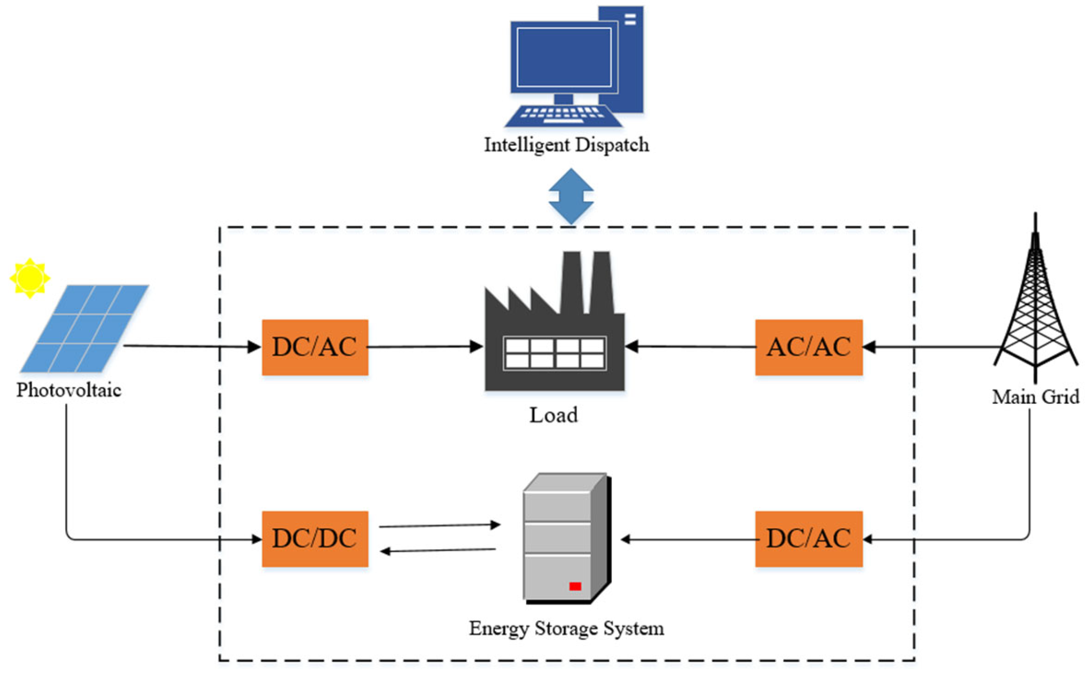
2. Problem Formulation and System Modeling

The Source-Grid-Load-Storage (S-G-L-S) architecture within the industrial plant is illustrated in Figure 1. The S-G-L-S system comprises a photovoltaic (PV), loads, grid connections, ESS, inverter modules, and an energy dispatch controller.

The economic cost of the plant’s electricity supply is influenced by the capital costs of the PV, ESS, and inverters. The installed PV capacity determines the hourly power generation: a higher installed capacity increases power generation but requires a higher upfront investment, whereas a lower capacity reduces costs but risks the generation of insufficient power to meet load demands. Similarly, the ESS capacity governs the energy storage scalability—larger capacities enable greater energy reserves but incur higher capital expenditures, and vice versa. Notably, the installed PV-ESS capacities directly impact the scheduling strategies during peak-flat-valley tariff periods. Therefore, optimizing both PV-ESS capacities is critical to balance the economic investment with the operational efficiency while ensuring load demand fulfillment.

2.1. Energy Storage Systems

The energy storage system (ESS) plays a critical role in energy dispatch operations, effectively smoothing renewable energy fluctuations [19], reducing peak-valley demand gaps, and lowering electricity costs. The ESS charging/discharging power at time slot t is denoted as $P_t^{ESS}$. The discharge mode ($P_t^{ESS}$ > 0) indicates the power supply to external loads, while the charge mode ($P_t^{ESS}$ < 0) represents the power absorption from either the grid or generation units. Mutual exclusivity between charging and discharging operations is enforced at all times. The power constraints of the ESS are formulated as

$$-P_{max}^{ESS}\le P_t^{ESS}\le P_{max}^{ESS}$$

(1)

where $P_{max}^{ESS}$ denotes the maximum allowable charging/discharging power of the ESS.

The state of charge (SOC) is a key indicator used to evaluate the charging and discharging state of a battery, as well as the remaining usable power [20]. Real-time SOC monitoring allows for the adjustment of ESS scheduling strategies, which in turn affects the electricity costs in industrial production. The SOC of the ESS at time t is denoted as $SO{C}_t$:

$$SO{C}_t=\left\{\begin{array}{ll}SO{C}_{t-1}-\alpha \cdot P_t^{ESS}\cdot {\eta }_{ch}^{ESS}\cdot \mathsf{\Delta }t/S^{ESS},& P_t^{ESS}\ge 0\\ SO{C}_{t-1}-\left(1-\alpha \right)\cdot P_t^{ESS}\cdot \mathsf{\Delta }t/\left(S^{ESS}\cdot {\eta }_{dis}^{ESS}\right),& P_t^{ESS}<0\end{array}\right.$$

(2)

Here, ${\eta }_{ch}^{ESS}$ and ${\eta }_{dis}^{ESS}$ represent the charging and discharging efficiencies of the ESS, while $S^{ESS}$ refers to the rated energy capacity of the ESS. When $\alpha =1$, the ESS operates in discharging mode, and when $\alpha =1$, the ESS operates in charging mode. $\mathsf{\Delta }t$ is the duration of time period t.

The SOC must be maintained within a safe range, with $SO{C}_{min}$ and $SO{C}_{max}$ representing the minimum and maximum values at which the ESS can operate properly, respectively.

$$SO{C}_{min}\le SO{C}_t\le SO{C}_{max}$$

(3)

The investment cost of the ESS is given by

$$C^{ESS}=\left(C_{\mathrm{u}\mathrm{n}\mathrm{i}\mathrm{t}}^{ESS}+C_{inst}^{ESS}+C_{ad}^{ESS}\right)\cdot S^{ESS}$$

(4)

where $S^{ESS}$ is the capacity of the ESS, $C_{unit}^{ESS}$ is the procurement cost per unit of capacity, $C_{inst}^{ESS}$ is the installation and integration cost per unit of capacity, and $C_{ad}^{ESS}$ is the operation and maintenance cost per unit of capacity.

2.2. Photovoltaics

Photovoltaic (PV) power generation is a solar energy technology that directly converts solar energy into electricity using the charge separation phenomenon in photovoltaic cells [21]. By applying a transparent conductive film to the surface of the PV panel, photons from sunlight excite electrons, generating a current that produces electricity. Solar radiation intensity and ambient temperature are the primary factors affecting PV power generation, which can be expressed by the following formula:

$$P_t^{PV}=P_{STC}{G}_{AC}{\displaystyle \frac{1+\delta \left(T_c-T_r\right)}{G_{STC}}}$$

(5)

$$T_c=T_e+30G_{AC}/1000$$

(6)

where $P_t^{PV}$ represents the PV output power; $P_{STC}$ is the maximum test power under the specific conditions; $G_{AC}$ is the radiation intensity; $\delta$ is the power temperature coefficient, typically −0.47%/K; $T_c$ is the operating temperature of the PV panels; $T_r$ is the reference temperature, typically 25 °C; $G_{STC}$ is the radiation intensity under standard test conditions, typically 1000 W/m²; and $T_e$ is the environmental temperature.

The installed PV capacity in industrial parks should account for the actual environmental constraints, and the installation area of PV modules should not exceed the maximum area available for panel installation in the park.

$$0<S^{PV}\le S_{max}^{PV}$$

(7)

The investment cost of PV is

$$C^{PV}=\left(C_{unit}^{PV}+C_{\mathrm{i}\mathrm{n}\mathrm{s}\mathrm{t}}^{PV}+C_{\mathrm{a}\mathrm{d}}^{PV}\right)\cdot S^{PV}$$

(8)

where $C_{unit}^{PV}$ is the cost of materials per unit area, $C_{\mathrm{i}\mathrm{n}\mathrm{s}\mathrm{t}}^{PV}$ is the cost of installation per unit area, and $C_{\mathrm{a}\mathrm{d}}^{PV}$ is the cost of maintenance and operation per unit area.

2.3. Main Grid

The S-G-L-S system in industrial parks is connected to the main grid (MG) through a transformer and operates in a grid-connected mode [22]. When the power supplied to the load by the PV-ESS is insufficient to support the normal operation of the load, power needs to be purchased from the MG to meet the load’s power requirements. When the amount of PV power generated exceeds the load’s electricity demand, the excess power is stored in the ESS to minimize curtailment losses [23]. The electric power corresponding to the amount of electricity purchased from the MG at time t is $P_t^{MG}$. The power purchased from the MG should satisfy the constraint

$$0\le P_t^{MG}\le P_{max}^{MG}$$

(9)

where $P_{max}^{MG}$ is the maximum power limit of the transformer. Industrial parks purchasing power from the MG need to consider the impact of time-sharing tariffs. The time-of-day tariffs for different moments of the day in Northeast China are shown below:

$$C_t^{MG}=\left\{\begin{array}{ll}0.628 \mathrm{C}\mathrm{N}\mathrm{Y}/\mathrm{K}\mathrm{W}.\mathrm{h}& 8\text{:}00\le t<12\text{:}00,17\text{:}00\le t<21\text{:}00\\ 0.529 \mathrm{C}\mathrm{N}\mathrm{Y}/\mathrm{K}\mathrm{W}.\mathrm{h}& 5\text{:}00\le t<8\text{:}00,12\text{:}00\le t<17\text{:}00,21\text{:}00\le t<22\text{:}00\\ 0.450 \mathrm{C}\mathrm{N}\mathrm{Y}/\mathrm{K}\mathrm{W}.\mathrm{h}& 22\text{:}00\le t<5\text{:}00\end{array}\right.$$

(10)

3. Solution Methodology

This study employed the TLCOA to configure the capacity of the PV-ESS in industrial parks and to co-optimize the S-G-L-S scheduling strategy. An industrial park served as the application scenario, providing contextual data such as load data, solar irradiance, and time-of-use tariffs. The iterative process described in this section, including population initialization and traversal of individuals, is part of the genetic algorithm (GA) used in the upper layer of the TLCOA to solve the optimization problem for an industrial park.

The concept of the TLCOA is illustrated in Figure 2. Firstly, the problem is analyzed and studied, a physical model is established, the objective function is set, the constraints are set, the data are pre-processed, and the operating parameters are set. Then the TLCOA is used to solve the problem, and the GA is used in the upper layer to solve the installed area of the PV and the capacity of the ESS, and the decision variables of the upper layer are passed into the lower layer. In the lower layer, MILP is used to solve the various time periods according to the decision variables of the upper layer. In the lower layer, MILP is used to solve the scheduling strategy for each time period according to the decision variables from the upper layer and evaluate the adaptability of the upper layer individuals; the adaptability value is returned to the upper layer to obtain the optimal individuals and optimal scheduling strategy. Finally, the performance of the algorithm is analyzed based on the results.

3.1. Decision Variables

In this study, the installed capacity of the PV ($S^{PV}$) and the configured capacity of the ESS ($S^{ESS}$) are taken as the upper level parameters of the SGLS system to be optimised, and the power supplied by the PV to the loads ($P_t^{\left(PV,L\right)}$), the charging power of the PV charging into the ESS ($P_t^{\left(PV,ESS\right)}$), the power supplied by the MG to the loads ($P_t^{\left(MG,L\right)}$), the charging power of the MG charging into the ESS ($P_t^{\left(MG,ESS\right)}$), and the power supplied by the ESS to the loads ($P_t^{\left(ESS,L\right)}$) at each time period were taken as the parameters to be optimized at the lower level. The significance of each variable is described in

Table 1. The meaning of the variables.

No.	Variable	Meaning
1	$S^{PV}$	Installed capacity of the PV
2	$S^{ESS}$	Installed capacity of the ESS
3	$P_t^{\left(PV,L\right)}$	Power from the PV to the load at time t
4	$P_t^{\left(PV,ESS\right)}$	Power from the PV to the ESS at time t
5	$P_t^{\left(MG,L\right)}$	Power from the MG to the ESS at time t
6	$P_t^{\left(MG,ESS\right)}$	Power from the MG to the ESS at time t
7	$P_t^{\left(ESS,L\right)}$	Power from the ESS to the load at time t
8	$P_t^L$	Load power consumption at time t
9	$P_t^{PV}$	Photovoltaic generation power at time t
10	$P_t^{ESS}$	ESS charging/discharging power at time t
11	$P_{max}^{ESS}$	Maximum power limit of the ESS
12	$P_t^{MG}$	Grid-supplied power at time t

.

3.2. Constraints

The stable operation of the plant load has to take into account the power balance constraints of the system [24]. The sum of the power supply from the PV-ESS and MG should meet the power requirements of the load:

$$P_t^{\left(L,PV\right)}+P_t^{\left(L,ESS\right)}+P_t^{\left(L,MG\right)}=P_t^L,t=1,2,\cdots T$$

(11)

where $P_t^{\left(L,PV\right)}$, $P_t^{\left(L,ESS\right)}$, and $P_t^{\left(L,MG\right)}$ are the electric power supplied to the load by the PV, ESS, and MG at time t, respectively. At moment t, the sum of the energy taken by the load and ESS from the PV system should be less than the PV output:

$$P_t^{\left(PV,L\right)}+P_t^{\left(PV,ESS\right)}\le P_t^{PV}$$

(12)

where $P_t^{\left(PV,L\right)}$ is the power supplied by the PV to the load at time t, $P_t^{\left(PV,L\right)}=P_t^{\left(L,PV\right)}$, and $P_t^{\left(PV,ESS\right)}$ is the charging power from the PV to the ESS at time t. At moment t, the power charged by the PV and MG to the ESS should be less than the upper limit of the rated power for charging the ESS, and the power discharged by the ESS to the load should be less than the upper limit of the rated power for discharging the ESS:

$$P_t^{\left(ESS,PV\right)}+P_t^{\left(ESS,MG\right)}=P_t^{ESS}\ge -P_{max}^{ESS}$$

(13)

$$P_t^{\left(ESS,L\right)}=P_t^{ESS}\le P_{max}^{ESS}$$

(14)

where $P_t^{\left(ESS,PV\right)}$ is the charging power obtained by the ESS from the PV at moment t, $P_t^{\left(ESS,MG\right)}$ is the charging power obtained by the ESS from the MG at moment t, and $P_t^{\left(ESS,L\right)}$ is the discharging power supplied by the ESS to the loads at moment t. For the ESS, the power to charge energy from the outside is negative and the power to discharge energy to the outside is positive [25].

$$P_t^{\left(ESS,PV\right)}=-P_t^{\left(PV,ESS\right)}$$

(15)

$$P_t^{\left(ESS,L\right)}=P_t^{\left(L,ESS\right)}$$

(16)

At moment t, the power supplied from the MG to the loads and ESS should be less than the upper limit of the rated power of the transformer:

$$P_t^{\left(MG,L\right)}+P_t^{\left(MG,ESC\right)}=P_t^{MG}\le P_{max}^{MG}$$

(17)

$P_t^{\left(MG,L\right)}$ is the power supplied by the MG to the load at time t, and $P_t^{\left(MG,ESS\right)}$ is the power charged by the MG to the ESS at time t.

$$P_t^{\left(ESS,MG\right)}=-P_t^{\left(MG,ESS\right)}$$

(18)

3.3. Objective Function

The optimization model’s core lies in its objective function. In this study, the objective function was formulated to minimize the plant’s total energy cost, which includes the capital costs of the PV system, ESS, power converters, and the operational costs of electricity consumption.

$$minCost=C_{mon}^{ESS}+C_{mon}^{PV}+C_{mon}^{CONV}+\sum _{t=0}^T{C}_t^{GD}\cdot P_t^{GD}\cdot \mathsf{\Delta }t$$

(19)

where $C_{mon}^{ESS}$, $C_{mon}^{PV}$, and $C_{mon}^{CONV}$ are the monthly investment costs for the ESS, PV, and converter, respectively; $C_t^{GD}$ is the time-of-use electricity price at time t; and $P_t^{GD}$ is the grid-supplied power at time t.

The costs and parameters of the PV system, ESS, and power converters are summarized in

Table 2. Equipment parameters and cost of construction.

Equipment Name	Optimization Scope	Construction Cost	Tenure (Years)
PV	$50–5\times {10}^3\hspace{0.17em}{\mathrm{m}}^2$	$8\times {10}^2\hspace{0.17em}\mathrm{C}\mathrm{N}\mathrm{Y}/{\mathrm{m}}^2$	20
ESS	$50–1\times {10}^3\hspace{0.17em}\mathrm{K}\mathrm{W}\mathrm{H}$	$1.1\hspace{0.17em}\mathrm{C}\mathrm{N}\mathrm{Y}/\mathrm{W}\mathrm{H}$	10
CONV	$50–5\times {10}^2\hspace{0.17em}\mathrm{K}\mathrm{W}$	$1.7\times {10}^2\hspace{0.17em}\mathrm{C}\mathrm{N}\mathrm{Y}/\mathrm{K}\mathrm{W}$	10

. In the actual construction of industrial parks, practical constraints must be considered. For the upper-layer optimization, the maximum available area for PV panel installation was set to $5\times {10}^3$ m², and the optimal range for the ESS rated capacity was 50–$1\times {10}^3$ kWh. For the lower-layer optimization, the power ratings of the PV inverters and ESS were constrained to 50–500 kW and 50–800 kW, respectively.

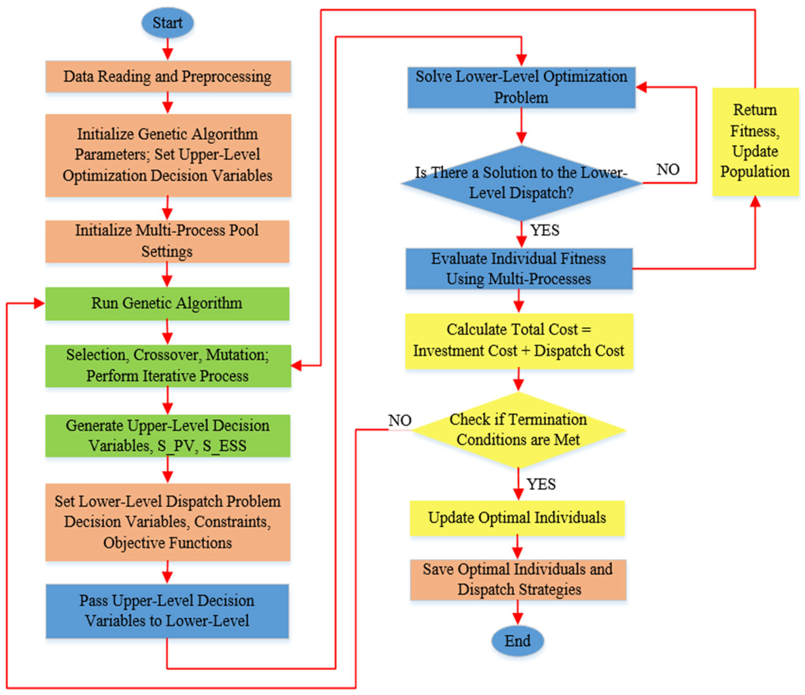
3.4. The Specific Solution Process

3.4.1. Overall Framework of TLCOA and Algorithm Flow

In this study, a TLCOA was used to allocate he PV-ESS capacity for the plant while solving the scheduling strategy that matches the capacity of the PV-ESS; the solution process is shown in Figure 3.

The TLCOA proposed in this study aims to simultaneously determine the optimal sizing of the PV and ESS (upper layer) and derive an economic scheduling strategy for the industrial load (lower layer). Figure 3 provides an overview of the TLCOA framework, showing how information flows between the two layers and how each layer interacts with the other.

In the industrial setting considered here, the investment costs for the PV–ESS and operational costs are closely intertwined. The upper layer focuses on long-term decisions—namely, the installed capacity of the PV-ESS. By searching a wide solution space, the GA balances the trade-offs between a larger PV–ESS capacity and a lower initial cost. Once the upper layer proposes a PV–ESS configuration, the lower layer solves a more detailed dispatch problem for each time step, taking into account the load demand, PV power generation, time-of-use tariffs, and the constraints on ESS charging and discharging.

This two-layer setup is crucial because planning (capacity sizing) and operational (energy dispatch) decisions are interdependent. A single-layer approach might overlook either the practical scheduling constraints or the long-term impact of the capacity choices. In contrast, the TLCOA framework iteratively refines both layers to achieve a globally better solution.

Before executing the algorithm, some data pre-processing work needs to be performed, including obtaining the hourly outdoor ambient temperature, solar radiation intensity, and meteorological parameters for Northeast China [26], and calculating the power generation per unit area of the photovoltaic panels. The actual operating data of the plant load and the power purchase price are collected from the power system at various times of the day. The acquired data are then normalized to create a standard dataset containing date, time, and period indices, and the dataset is checked for negative and missing values to ensure its validity.

3.4.2. Upper-Layer GA for PV–ESS Capacity Optimization

The goal of the upper-level optimization is to determine the optimal installed capacity of the PV-ESS to minimize the total system cost. The population is initially generated, and its quality is improved using methods such as Random Generation (RG), Heuristic Generation (HG), and Latin Hypercube Sampling (LHS) [27] to produce diverse initial solutions that satisfy the initial constraints. Selection, crossover, and mutation are performed, and the lower-level scheduling optimization function is invoked as the fitness function to compute individual fitness. After multiple rounds of iterative evolution, the optimal solution for the upper-level decision variables is obtained.

First, according to the constraint ranges of the decision variables ${\mathrm{S}}^{\mathrm{P}\mathrm{V}}$ and ${\mathrm{S}}^{\mathrm{E}\mathrm{S}\mathrm{S}}$ given in Table 2 of Section 3.3, we encode them accordingly. Each individual in the population is represented as ind:

$$\mathrm{i}\mathrm{n}\mathrm{d}=({\mathrm{S}}^{\mathrm{P}\mathrm{V}},{\mathrm{S}}^{\mathrm{E}\mathrm{S}\mathrm{S}})$$

(20)

Next, the population is initialized. The RG (Random Generation) method uses random sampling to produce a subset of individuals, thus maintaining broad coverage of the search space. The HG (Heuristic Generation) method relies on heuristic rules: in this study, it was set so that the peak PV generation exceeds the peak load demand, and the ESS can store enough energy to meet peak-period load requirements. The LHS (Latin Hypercube Sampling) method divides the variable ranges into equal strata and systematically samples within each stratum, thereby enhancing sample coverage. By combining these three approaches, the initial population benefits from both randomness and heuristic insights, reducing the risk of becoming trapped in local optima.

Each GA individual $\mathrm{i}\mathrm{n}\mathrm{d}=({\mathrm{S}}^{\mathrm{P}\mathrm{V}},{\mathrm{S}}^{\mathrm{E}\mathrm{S}\mathrm{S}})$ undergoes a lower-layer dispatch optimization (MILP) to compute the corresponding total cost (investment + dispatch cost). The resulting total cost is then transformed into a fitness value $f$:

$$f\left(t\right)={\displaystyle \frac{1}{C^{invest}+C_t^{dispatch}}}$$

(21)

$$C^{invest}=C_{mon}^{ESS}+C_{mon}^{PV}+C_{mon}^{CONV}$$

(22)

$$C_t^{dispatch}=\sum _{t=0}^T{C}_t^{MG}\cdot P_t^{MG}\cdot \mathsf{\Delta }t$$

(23)

where $C^{invest}$ is the investment cost and $C_t^{dispatch}$ is the dispatch cost.

A lower total cost yields a higher fitness, guiding the GA to favor configurations that combine reduced capital expenditure (capex) and minimized electricity purchase cost. Once the fitness scores are obtained, the GA applies standard genetic operators to improve the population iteratively. By applying tournament selection, the more adaptive individuals are chosen for reproduction. Then, the decision variables of the two selected parents are combined to generate offspring, as shown in Equations (24) and (25).

$${\mathrm{S}}^{\mathrm{P}\mathrm{V}}\left(child\right)=\alpha {\mathrm{S}}^{\mathrm{P}\mathrm{V}}\left(parent1\right)+(1-\alpha ){\mathrm{S}}^{\mathrm{P}\mathrm{V}}\left(parent2\right)$$

(24)

$${\mathrm{S}}^{ESS}\left(child\right)=\alpha {\mathrm{S}}^{ESS}\left(parent1\right)+(1-\alpha ){\mathrm{S}}^{ESS}\left(parent2\right)$$

(25)

where $\alpha$ is a randomly chosen coefficient in [0, 1]. A small random mutation is introduced into each individual, as shown in Equation (26), to ensure population diversity and prevent the search from stagnating.

$${\mathrm{S}}^{\mathrm{P}\mathrm{V}}\left(child\right)={\mathrm{S}}^{\mathrm{P}\mathrm{V}}\left(child\right)\pm {\delta }_p$$

(26)

$${\mathrm{S}}^{ESS}\left(child\right)={\mathrm{S}}^{ESS}\left(child\right)\pm {\delta }_e$$

(27)

where ${\delta }_p$ and ${\delta }_e$ are mutation magnitudes constrained by the feasible ranges.

After each generation, a new population is formed, comprising the best individuals carried over (elitism) and newly generated offspring. The algorithm repeats selection, crossover, mutation, and re-evaluation until the termination condition is met, at which point, the genetic algorithm finds the best individual.

3.4.3. Lower-Layer MILP for Energy Dispatch

The decision variables for the PV installed capacity and ESS capacity from the upper layer are passed to the lower layer to optimize the distribution of power between the PV, ESS, and MG across each time period. The lower-level dispatch operations must satisfy the energy balance constraints, SOC constraints for energy storage, charge/discharge mutual exclusion constraints, PV generation allocation constraints, and charge/discharge power limitations [28].

Based on the constraints in Section 3.2 and the objective function in Section 3.3, MILP is solved using the standard solver CPLEX. The lower layer calculates the dispatch cost for each individual passed down from the upper layer; summing the dispatch cost and the investment cost yields the total cost, which serves as that GA individual’s fitness measure. The algorithm iteratively updates the fitness and re-solves until convergence. By coordinating both layers, the TLCOA not only provides capacity decisions that minimize capital and operating expenditures but also generates a practical, time-indexed dispatch plan that captures actual load demands, PV availability, and battery storage constraints.

The inverse of the total cost is used as the fitness value to guide the upper-level GA in its evolutionary search. The lower-level scheduling uses MILP to calculate the scheduling cost based on the decision variables $S^{PV}$ and $S^{ESS}$ passed from the upper level. The upper-level GA is integrated with the lower-level scheduling through the fitness function, achieving collaborative optimization of PV-ESS capacity allocation and power scheduling via the feedback mechanism.

The key parameters analysis for the TLCOA algorithm are listed in

Table A1. Key parameter analysis for the TLCOA algorithm.

Parameter	Value/Range	Rationale and Justification
Population Size (GA)	100	(1) Coverage vs. Efficiency: A population of 100 maintains sufficient exploration of the search space without excessively prolonging the evaluation. (2) Leverages parallel fitness evaluation to handle the per-individual MILP cost.
Number of Generations (GA)	50	(1) Search Depth: Fifty generations allow the GA to refine solutions adequately while keeping the runtime manageable. (2) Empirical tests showed minor improvements after ~40 generations.
Crossover Probability (GA)	0.7	(1) Population Diversity: A moderately high crossover rate (0.6–0.9) is typical to encourage the recombination of promising traits. (2) Balances exploration (varied offspring) and exploitation (retaining good genetic segments).
Mutation Probability (GA)	0.2	(1) Avoid Premature Convergence: A 20% mutation rate ensures continued genetic diversity, preventing stagnation in local minima. (2) A higher mutation rate might destabilize convergence; a lower rate could limit exploration.
Time Horizon and Step	24 h @ 1 h step	(1) Granularity vs. Complexity: A 1 h time-step yields a tractable MILP size while capturing daily load patterns. (2) Smaller steps increase accuracy but raise solver complexity.
${\eta }_{ch}^{ESS}{,\eta }_{ch}^{ESS}$	0.95, 0.95	(1) Round-Trip Efficiency: A 95% charging/discharging efficiency approximates the typical Li-ion battery performance. (2) Could be tuned for other battery chemistries if needed.

of Appendix A.

3.4.4. Implementation Details and Parallel Computing

To address the high time complexity associated with large data dimensions and population sizes in fitness evaluation, a parallel assessment method is employed to evaluate individuals using the fitness function, as shown in Figure 4. Figure 4a shows the process of serially evaluating the fitness in the main process, while Figure 4b shows the process of parallel fitness evaluation across multiple subprocesses. The adaptation calculation tasks are distributed to multiple subprocesses via the process pool, with each subprocess independently executing the fitness function. The results are then aggregated in the main process to update the population’s fitness values, reducing the time overhead of the adaptation evaluation. Through continuous iterations, the optimal PV-ESS capacity is determined, along with the scheduling strategies for different time periods based on the corresponding capacities.

The pseudocode of the TLCOA algorithm is given below (Algorithm 1).

Algorithm 1. TLCOA: Two-Layer Cooperative Optimization for PV–ESS Sizing and Dispatch

# Upper Layer: Genetic Algorithm (GA) # Lower Layer: Mixed-Integer Linear Programming (MILP) # Parallel Fitness Evaluation: each population member is evaluated in parallel. Procedure TLCOA_Main:   1. (prices_df, pv_output_df, load_df) ← read_and_preprocess(“data_file.csv”)   2. Initialize global data for parallel processes (init_pool_globals).   3. (toolbox, var_bounds, avg_load, pool) ← setup_genetic_algorithm()   4. (best_ind, logbook, hof) ← run_genetic_algorithm(toolbox)   5. extract_and_visualize_results(best_ind)   6. pool.close(), pool.join() End Procedure -------------------------------------------------------------------------------- Function run_genetic_algorithm(toolbox) → (best_ind, logbook, hof):   1. population ← toolbox.population()   2. ngen ← 500, cxpb ← 0.7, mutpb ← 0.2   3. hof ← HallOfFame(1)   4. stats ← define_statistics(…)   5. (population, logbook) ← eaSimple(      population, toolbox,      cxpb = cxpb, mutpb = mutpb,      ngen = ngen, stats = stats,      halloffame = hof, verbose = True    )   6. best_ind ← hof[0]   # best (S_PV, S_ESS) solution   7. return (best_ind, logbook, hof) End Function -------------------------------------------------------------------------------- Function evaluate(individual) → fitness:   # individual = (S_PV, S_ESS)   1. investment_cost ← compute_investment(S_PV, S_ESS)   2. (dispatch_cost, _) ← optimize_dispatch(S_PV, S_ESS, global_data, …)   3. if dispatch_cost = ∞ then     return large_value   4. total_cost ← investment_cost + dispatch_cost   5. return total_cost End Function -------------------------------------------------------------------------------- Function optimize_dispatch(S_PV, S_ESS, prices_df, pv_output_df, load_df, …) → (cost, dispatch_df):   1. prob ← create MILP problem (MINIMIZE total electricity cost)   2. for each time slot t in load_df:     - Define variables: P_PV_load[t], P_grid_load[t], P_ESS_load[t], etc.     - Enforce constraints:     (a) Load balance: P_PV_load[t] + P_grid_load[t] + P_ESS_load[t] = Load[t]     (b) PV allocation: P_PV_load[t] + P_PV_ESS[t] ≤ S_PV * PV_output[t]     (c) ESS SOC: E_ESS[t+1] = E_ESS[t] + …     (d) Charge/discharge limits and binary constraints for mutual exclusivity   3. Add objective function: minimize ∑(price[t] × grid_power[t]) [± any sell/buy terms]   4. prob.solve()   5. if solution is not Optimal: return (∞, None)   6. cost ← value(prob.objective)   7. dispatch_df ← extract_decision_variables(prob)   8. return (cost, dispatch_df) End Function

4. Validation and Analysis of Case Studies

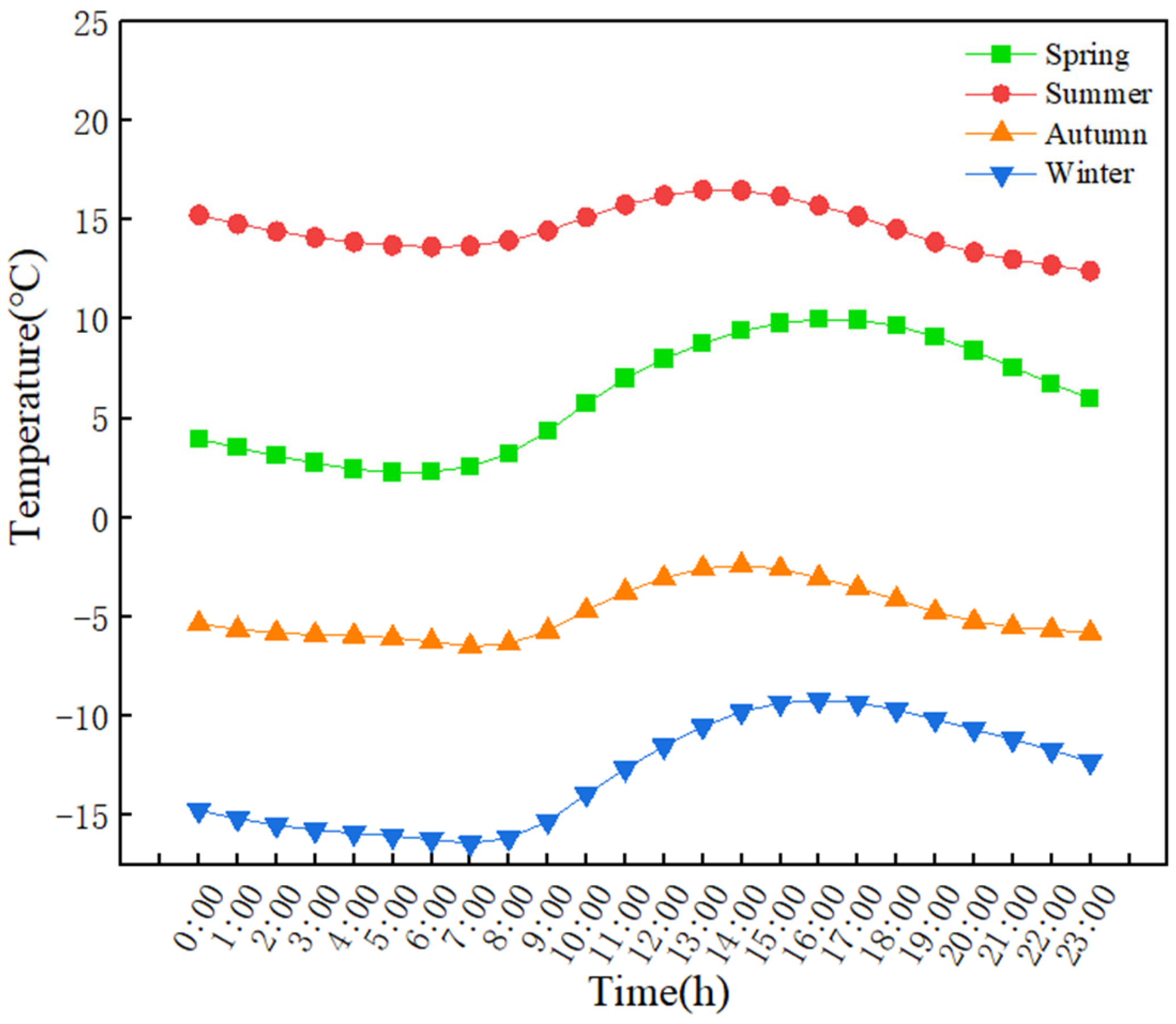
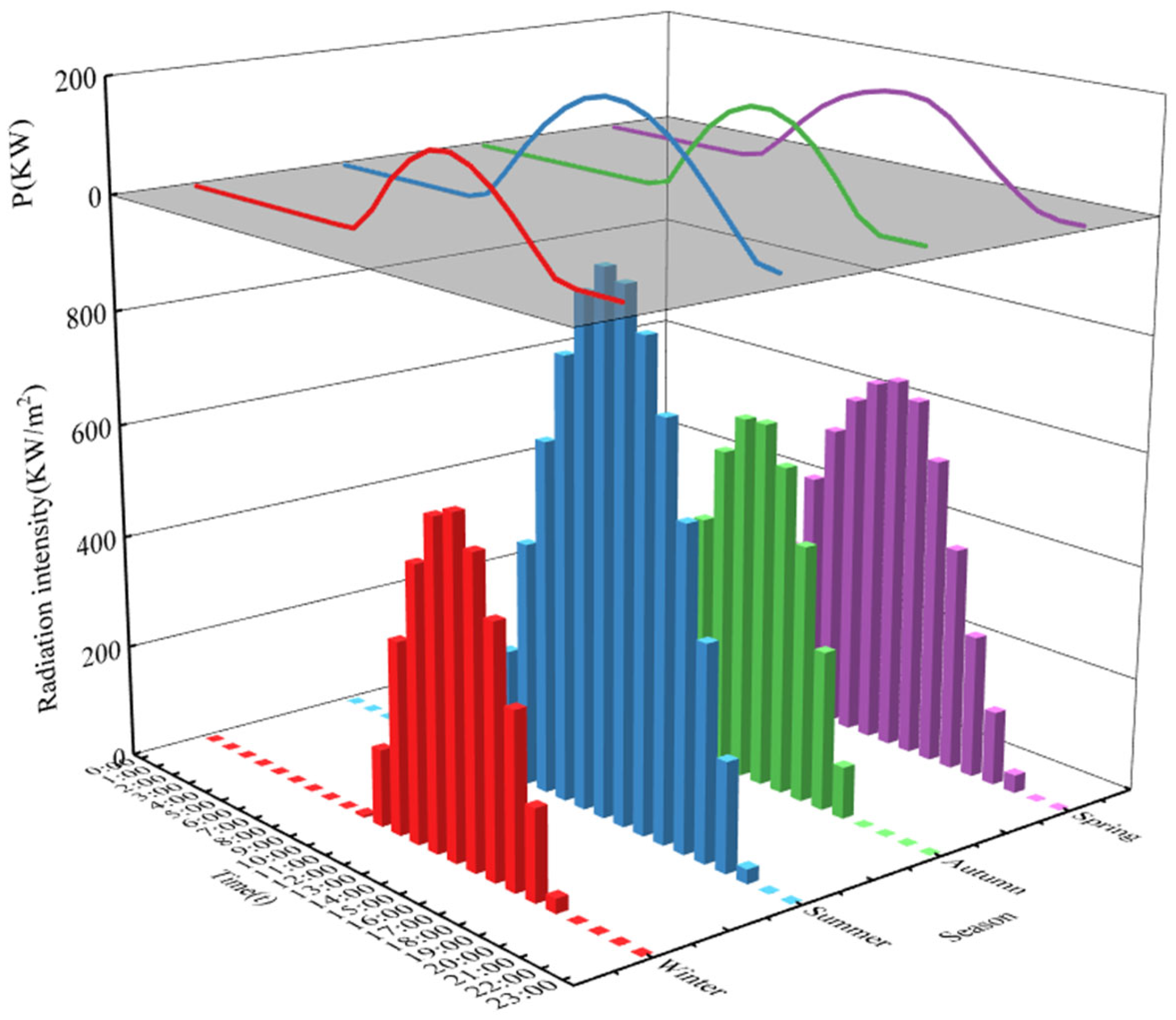
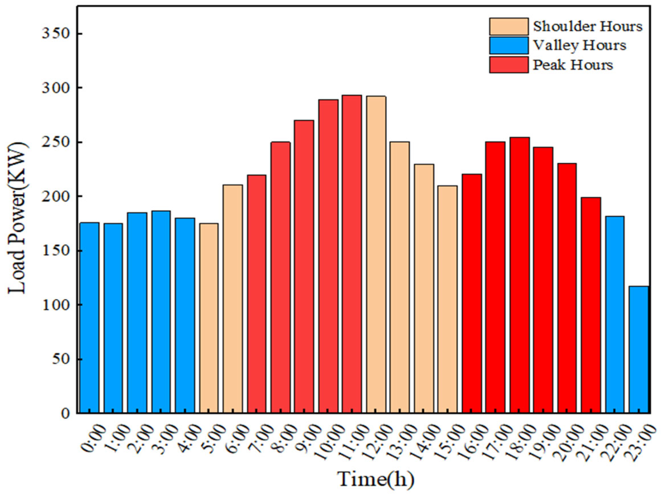
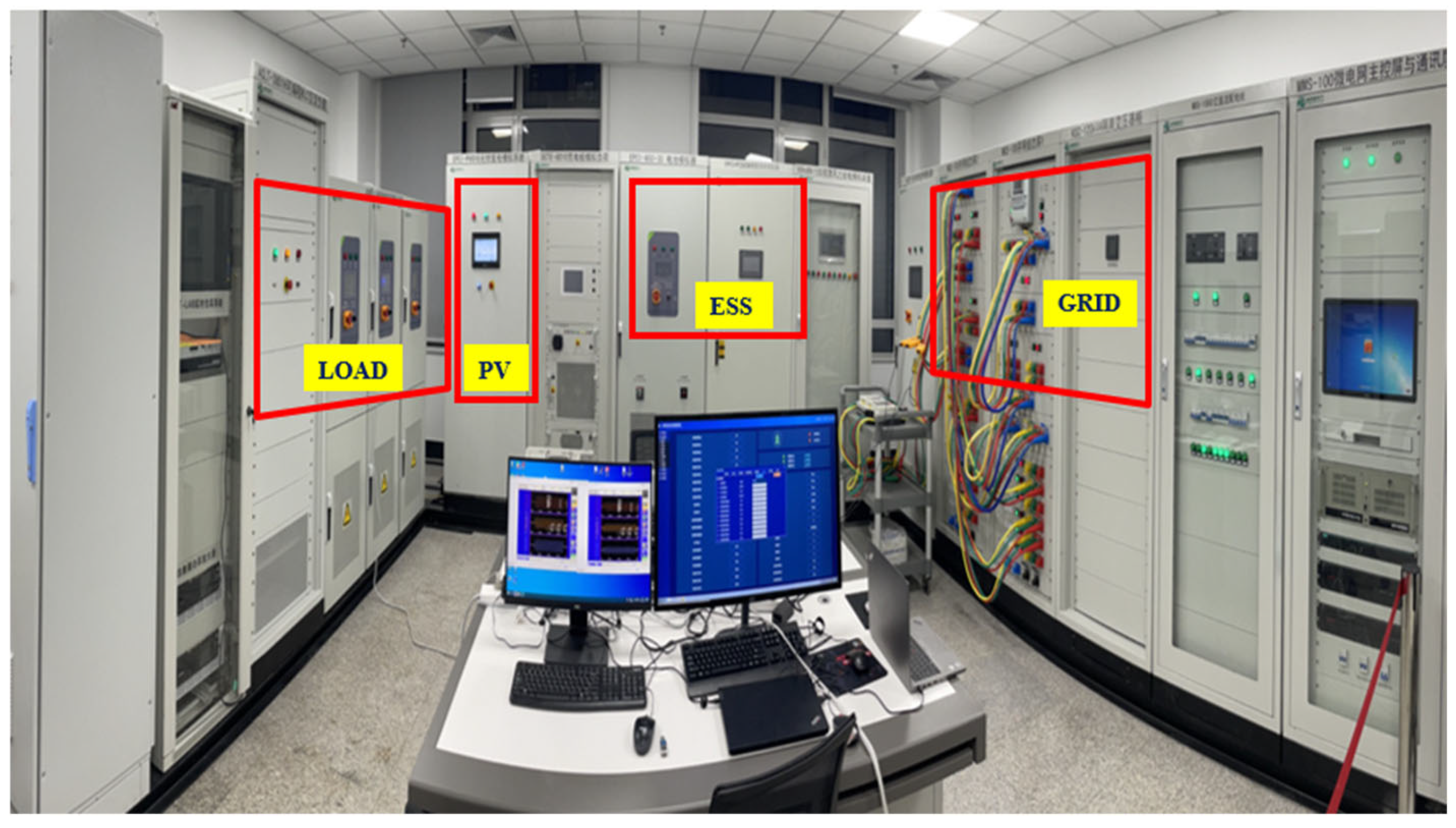
4.1. Case Description

In this study, solar irradiance data from a region in Northeast China were utilized to establish a photovoltaic (PV) power generation model. Figure 5 illustrates the hourly variations of outdoor environmental factors on a typical day in each season. As shown in Figure 5, the outdoor temperature exhibited distinct seasonal patterns, with summer temperatures averaging around 15 °C and winter temperatures ranging between −10 °C and −15 °C, indicating a significant temperature difference between summer and winter.

Figure 6 illustrates the variations in outdoor solar irradiance on a typical day across spring, summer, autumn, and winter. As shown in the figure, the diurnal patterns of irradiance were consistent across all seasons, exhibiting a bell-shaped curve. Irradiance gradually increased in the morning, peaked around 14:00, and then decreased in the afternoon, dropping to zero after sunset. This demonstrates the clear diurnal intermittency of solar resources. The maximum irradiance reached 943.6 W/m² in summer and 593.9 W/m² in winter, with winter irradiance being approximately 63% of summer levels. Similarly, PV power generation followed the same trend as irradiance, with peak power reaching 210.5 KW in summer and 146.7 KW in winter. The winter PV power was about 70% of summer levels, indicating significant seasonal variability in PV performance.

Load data from a factory in Northeast China were utilized to establish a load model. Figure 7 presents the daily power consumption histogram of the factory’s workshop load. As shown in the figure, the workshop’s production load exhibited relatively stable power consumption. The power consumption during daytime peak hours was significantly higher than during nighttime valley hours, indicating a pronounced peak–valley difference in the factory’s load profile.

The Source–Grid–Load–Storage laboratory is illustrated in Figure 8. We fed the real-world power data we obtained into this laboratory for validation to ensure that our algorithm was not confined to a purely simulated environment and can function effectively under real-world conditions.

4.2. Validation of the TLCOA

This section presents a comparative analysis of the two-layer cooperative optimization approach (TLCOA), genetic algorithm (GA), and data-driven algorithm (DDA) proposed in this study.

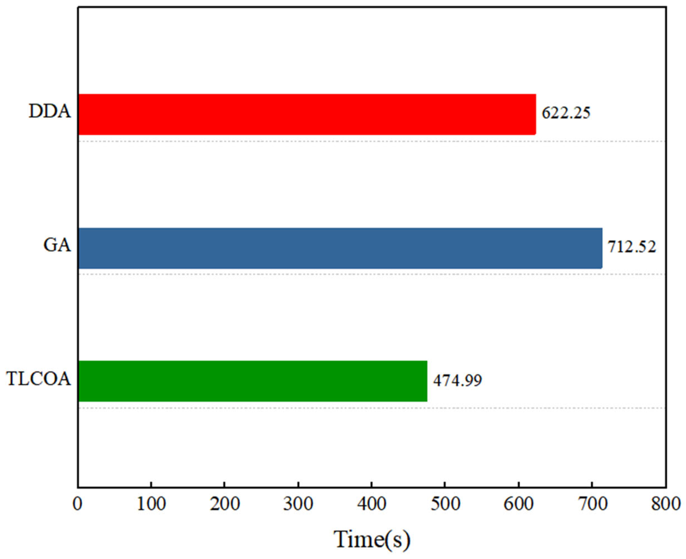
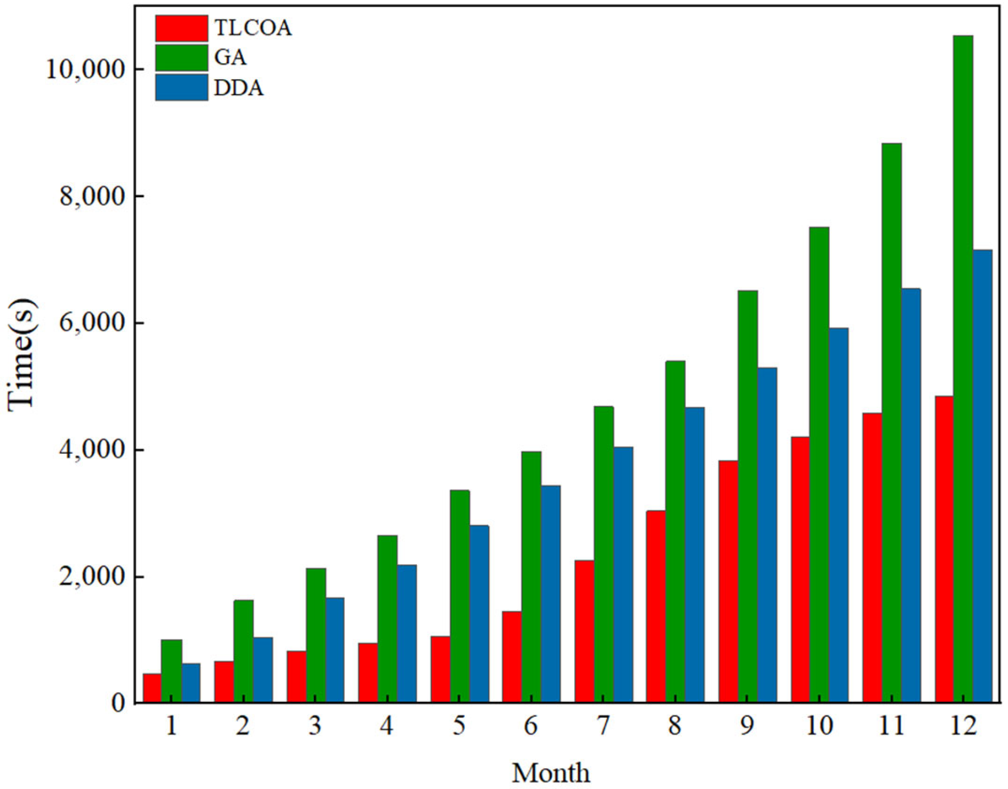
4.2.1. Comparison of Solution Time

Figure 9 shows the computation time for the three methods. The calculation times for the TLCOA, GA, and DDA were 474.99, 712.52, and 622.25 s, respectively. The comparison showed that the TLCOA, which employs parallel fitness evaluation, reduced the computation time by 33.33% compared to the GA and 23.68% compared to the DDA.

In order to verify the performance advantages of the TLCOA algorithm in large-scale data scenarios, we designed a comparative experiment in which the dataset size was gradually increased on a monthly basis, as shown in Figure 10, and then examined how the running times of the TLCOA, GA, and DDA vary with different data volumes. The comparison of running times for these three algorithms under large-scale data conditions is illustrated in Figure 11. Owing to its use of multi-process parallel computing, the TLCOA achieved the shortest running time of 1647.72 s, whereas the DDA algorithm took 7467.00 s, and the GA algorithm required the longest time at 8550.24 s.

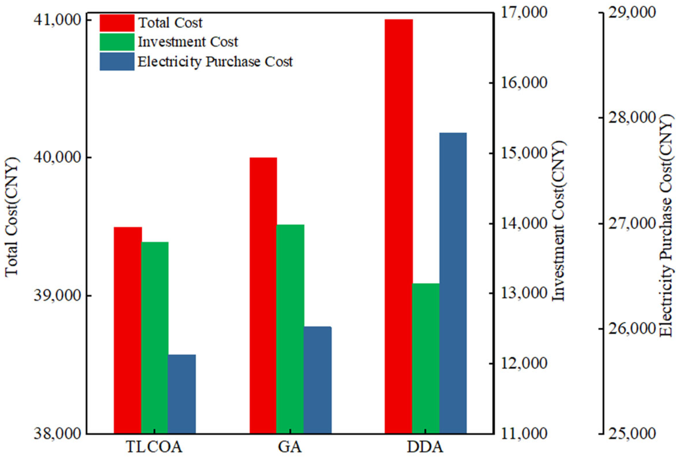
4.2.2. Comparison of Economic Benefits

In terms of economic benefits, the capacities of the optical storage systems designed by the three methods are presented in

Table 3. Installed capacity of PV-ESS from different methods.

Parameter	TLCOA	GA	DDA
$\mathrm{ESS} \mathrm{capacity} (\mathrm{K}\mathrm{W}\mathrm{H}$)	998	1000	1099
$\mathrm{PV} \mathrm{capacity} ({\mathrm{m}}^2$)	1376	1444	921

. The electricity costs for the three methods are shown in Figure 12. The total electricity costs for the TLCOA, GA, and DDA were CNY 39,497.9, CNY 40,001.1, and CNY 41,005.1, respectively. Among these, the investment and construction costs of the PV-ESS for the TLCOA, GA, and DDA were CNY 13,740.3, CNY 13,981.9, and CNY 13,144.2, respectively. The monthly purchased electricity costs for the TLCOA, GA, and DDA were CNY 25,757.4, CNY 26,019.2, and CNY 27,860.9, respectively. The calculations show that the TLCOA saved CNY 62,832 and CNY 504,840 in electricity purchase costs over the effective working life of the PV panels compared to the GA and DDA, respectively.

The long-term economic benefits of a factory are vital for maintaining normal production operations.

Table 4. Investment cost, electricity purchase cost, maintenance cost, annual savings, and expected payback period under different algorithms.

Method	TLCOA	GA	DDA
Investment Cost (103 CNY)	2199.57	2255.68	1946.00
Annual Operational Cost (CNY)	309.09	312.23	334.33
Annual Maintenance Cost (CNY)	2474.93	2544.6	2130.22
Payback Period (Years)	3.22	3.31	2.96

presents an analysis, from a long-term perspective, of the investment cost, electricity purchase cost, maintenance cost, annual savings, and estimated payback period under the different algorithms. The results indicate that the payback periods for the TLCOA, GA, and DDA were 3.22 years, 3.31 years, and 2.96 years, respectively, suggesting that these three methods have relatively close payback times. However, from a long-term viewpoint, after reaching the break-even point, the TLCOA algorithm provided higher benefits.

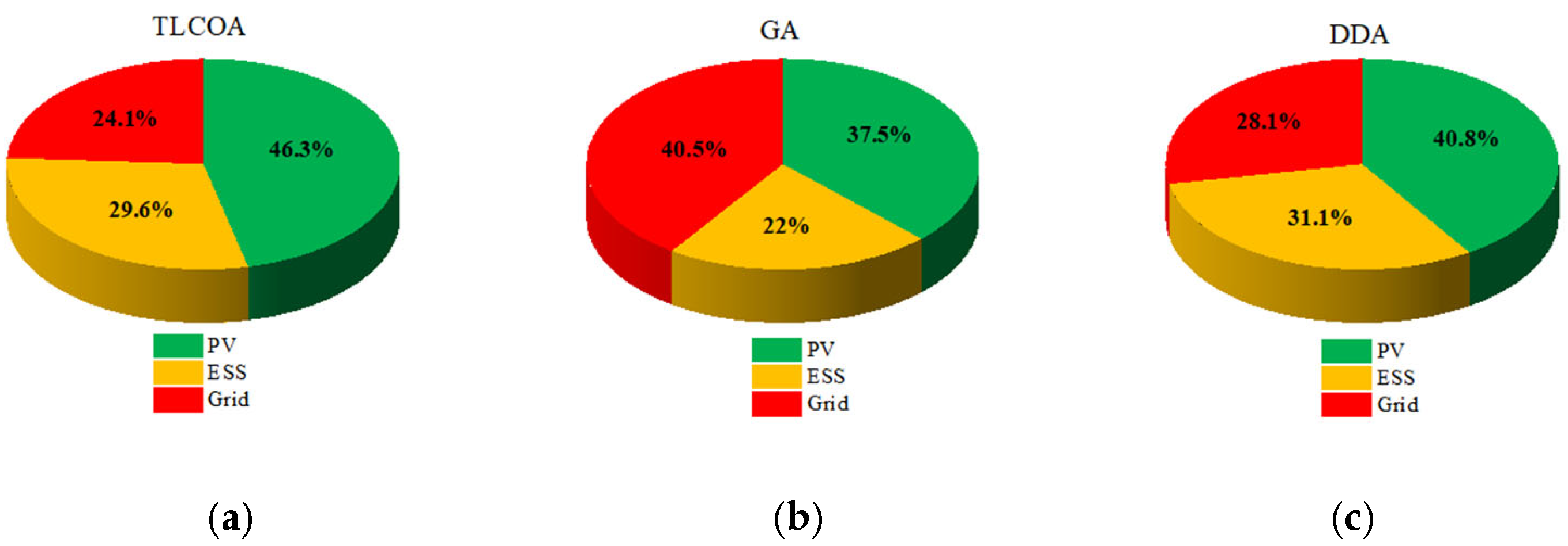
4.2.3. Comparison of Renewable Energy Utilization Rate

Figure 13 illustrates the intra-day energy supply distribution from the PV system, ESS, and main grid (MG) to the load under the TLCOA, GA, and DDA. For the TLCOA, the contributions of the PV, ESS, and MG to the load were 46.34%, 29.59%, and 24.07%, respectively. Under the GA, these values were 40.85%, 31.09%, and 28.06%, while under the DDA, they were 37.55%, 21.98%, and 40.47%. Among the three methods, the TLCOA achieved the highest PV-ESS utilization rate at 75.93%, whereas the DDA exhibited the lowest at 59.53%. These results demonstrate the superiority of the TLCOA in renewable energy utilization, effectively enhancing the integration of renewable energy while meeting the plant’s load demand, which aligns with the algorithm’s design objectives.

4.2.4. Analysis of System Stability

In terms of integrated system performance, the interaction between the PV, ESS, loads, and MG after using the TLCOA is shown in Figure 11. The PV, ESS, and MG power supply met the load’s electricity demand, and the MG gave priority to supplying power to the load during the valley hours (22:00–5:00) at night when the cost of purchasing electricity is lower, while the MG charged the ESS at the same time during the hours when the price of electricity is lower. During the daytime peak hours (8:00–12:00), when power purchase costs are high, power was mainly supplied to the loads by the PV, while the excess power was deposited into the ESS at the peak PV output moments, and during the nighttime peak hours (17:00–21:00), when power purchase costs are high, power was mainly supplied to the loads by the ESS. During the shoulder hours periods (5:00–8:00, 12:00–17:00, 21:00–22:00), the system was mainly powered by the PV and ESS. This scheduling strategy shaves peaks and fills valleys to supply power to the loads by taking into account the time-sharing tariffs during peak and valley hours in order to reduce electricity costs for the plant.

In terms of system stability, Figure 14 illustrates the interactions among the source, grid, load, and storage (S-G-L-S) using the TLCOA algorithm under different seasonal conditions. Overall, with the TLCOA in spring, summer, autumn, and winter, the power supplied by the PV, ESS, and MG was capable of meeting the load demands. Specifically, the TLCOA scheduling strategy tended to charge the ESS at night, during the valley time period (22:00–05:00) when electricity prices are lower, with the main grid (MG) supplying both the load and the ESS. During the day (08:00–12:00), when electricity purchase costs are higher, the load was primarily powered by PV, and any surplus PV generation was stored in the ESS. During the high-cost evening peak (17:00–21:00), the ESS mainly supplied the load. During shoulder periods (05:00–08:00, 12:00–17:00, and 21:00–22:00), the load was predominantly powered by a combination of the PV and ESS. By leveraging peak–valley TOU tariffs, this strategy “shaves peaks and fills valleys” to reduce the factory’s electricity costs.

In spring and autumn, the PV generation did not differ significantly, so the scheduling strategies remained relatively consistent. In contrast, summer features higher solar irradiance and ambient temperatures, thus enabling greater PV generation. Surplus daytime generation was stored for use during nighttime hours (21:00–23:00). In winter, solar irradiance is lower and temperatures are colder, resulting in reduced PV output. Consequently, less PV power was stored during the day, and the evening period (19:00–23:00) required increased electricity purchases from the grid to maintain load stability. Under stable load conditions, winter’s electricity purchase cost surpassed that in summer by CNY 71,698.13.

5. Conclusions

To achieve stable load operation and minimize electricity costs in industrial parks, this paper proposes a TLCOA for optimizing upper-level equipment configuration and lower-level operating parameters using real power system and plant load data. The key findings can be summarized as follows:

(1)

By employing a parallel multi-process solving strategy in the TLCOA, the time required to find the optimal scheduling solution was reduced by 33.33% and 23.68%, compared to the GA and DDA, significantly improving the solving efficiency.

(2)

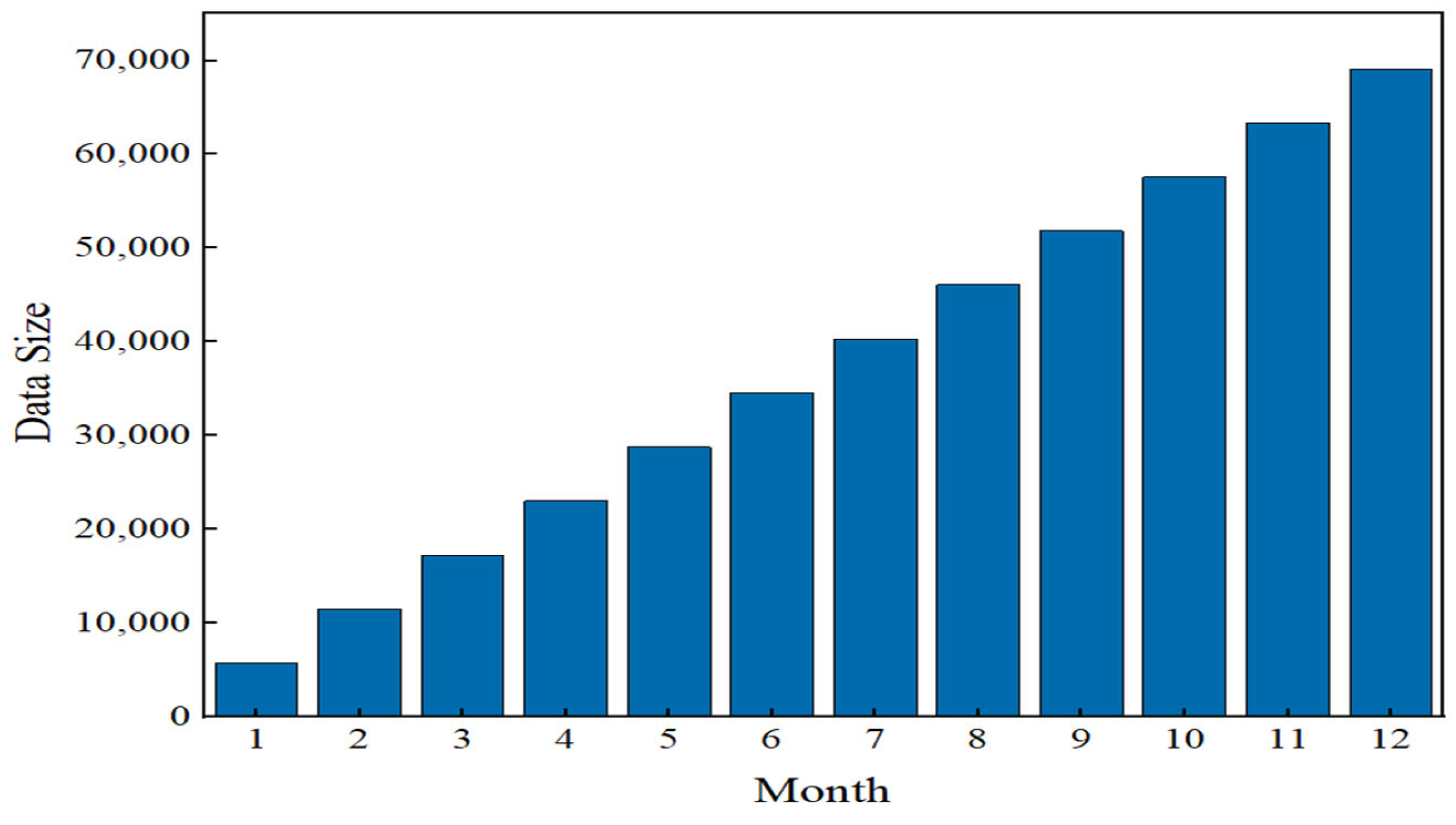
The experimental results showed that, compared to the single-layer GA algorithm and the DDA algorithm, TLCOA exhibited significant advantages in handling large-scale datasets. Nonetheless, given the high efficiency required for industrial energy dispatch, there remains room for further enhancement of the TLCOA algorithm. Future studies could explore reinforcement learning-based search strategies or other hybrid methods to improve the energy dispatch efficiency.

(3)

A TLCOA was used to model the investment in the PV-ESS for the plant. The PV area was 1376 m² and the ESS capacity was 998 kWh, resulting in a 1.73% reduction in investment costs and a 7.55% reduction in purchased power costs. As a result, the economic cost of energy use in the plant was significantly reduced.

(4)

From a long-term economic perspective, this study analyzed the payback period for a factory’s investment in a PV–ESS system. With the TLCOA, the payback period was 3.22 years, after which, the factory attained the greatest savings in electricity purchases, thus maximizing economic returns. This study offers a reliable plan for implementing PV–ESS systems in industrial facilities.

(5)

By scheduling the load energy supply using the TLCOA, the PV, ESS, and MG supplied 46.34%, 29.59%, and 24.07% of the load, respectively. The PV power supply increased by 8.79%, significantly improving the utilization rate of renewable energy.

(6)

Based on the comprehensive system performance analysis, after adopting the TLCOA, the S-G-L-S system provided a stable power supply to the loads and could adjust the power supply strategy according to time-of-day tariffs, achieving “peak shaving and valley filling”.

Regarding system stability, the scheduling strategy obtained via the TLCOA algorithm adapted well to environmental variations across the spring, summer, autumn, and winter. This ensures a stable power supply to the loads while also achieving “peak shaving and valley filling”.

This study offers insights into the construction of optical storage systems for high power-consuming enterprises. The TLCOA considers system stability, solution efficiency, economic cost, and renewable energy utilization, providing an optimized solution for complex energy systems.

References

1. Zhao, X.; Ma, X.; Chen, B.; Shang, Y.; Song, M. Challenges toward Carbon Neutrality in China: Strategies and Countermeasures. Resour. Conserv. Recycl. 2022, 176, 105959. [Google Scholar] [CrossRef]
2. Shao, T.; Pan, X.; Li, X.; Zhou, S.; Zhang, S.; Chen, W. China’s Industrial Decarbonization in the Context of Carbon Neutrality: A Sub-Sectoral Analysis Based on Integrated Modelling. Renew. Sustain. Energy Rev. 2022, 170, 112992. [Google Scholar] [CrossRef]
3. Wang, S.; Yue, Y.; Cai, S.; Li, X.; Chen, C.; Zhao, H.; Li, T. A Comprehensive Survey of the Application of Swarm Intelligent Optimization Algorithm in Photovoltaic Energy Storage Systems. Sci. Rep. 2024, 14, 17958. [Google Scholar] [CrossRef] [PubMed]
4. Li, S.; Xu, Q.; Yang, Y.; Xia, Y.; Hua, K. Study on Distributed Renewable Energy Generation Aggregation Application Based on Energy Storage. Int. J. Electr. Power Energy Syst. 2024, 158, 109935. [Google Scholar] [CrossRef]
5. Yang, C.; Lin, Z.; Huang, K.; Wu, D.; Gui, W. Manifold Embedding Stationary Subspace Analysis for Nonstationary Process Monitoring with Industrial Applications. J. Process Control 2024, 140, 103262. [Google Scholar] [CrossRef]
6. Fan, G.-F.; Feng, Y.-W.; Peng, L.-L.; Huang, H.-P.; Hong, W.-C. Uncertainty Analysis of Photovoltaic Power Generation System and Intelligent Coupling Prediction. Renew. Energy 2024, 234, 121174. [Google Scholar] [CrossRef]
7. Xie, L.; Xiang, Y.; Xu, X.; Wang, S.; Li, Q.; Liu, F.; Liu, J. Optimal Planning of Energy Storage in Distribution Feeders Considering Economy and Reliability. Energy Tech. 2024, 12, 2400200. [Google Scholar] [CrossRef]
8. Jiang, C.; Mao, Y.; Chai, Y.; Yu, M. Day-ahead Renewable Scenario Forecasts Based on Generative Adversarial Networks. Int. J. Energy Res. 2021, 45, 7572–7587. [Google Scholar] [CrossRef]
9. Zhu, D.; Liu, W.; Hu, Y.; Wang, W. A Practical Load-Source Coordinative Method for Further Reducing Curtailed Wind Power in China with Energy-Intensive Loads. Energies 2018, 11, 2925. [Google Scholar] [CrossRef]
10. Xu, M.; Li, W.; Feng, Z.; Bai, W.; Jia, L.; Wei, Z. Economic Dispatch Model of High Proportional New Energy Grid-Connected Consumption Considering Source Load Uncertainty. Energies 2023, 16, 1696. [Google Scholar] [CrossRef]
11. Li, L.; Cao, X. Comprehensive Effectiveness Assessment of Energy Storage Incentive Mechanisms for PV-ESS Projects Based on Compound Real Options. Energy 2022, 239, 121902. [Google Scholar] [CrossRef]
12. Guo, Z.; Zhang, X.; Li, M.; Wang, H.; Han, F.; Fu, X.; Wang, J. Control and Capacity Planning for Energy Storage Systems to Enhance the Stability of Renewable Generation Under Weak Grids. EBSCOhost. Available online: https://openurl.ebsco.com/contentitem/doi:10.1049%2Frpg2.12424?sid=ebsco:plink:crawler&id=ebsco:doi:10.1049%2Frpg2.12424 (accessed on 11 February 2025).
13. Zamanpour, K.; Vaziri Rad, M.A.; Saberi, N.; Fereidooni, L.; Kasaeian, A. Techno-Economic Comparison of Dispatch Strategies for Stand-Alone Industrial Demand Integrated with Fossil and Renewable Energy Resources. Energy Rep. 2023, 10, 2962–2981. [Google Scholar] [CrossRef]
14. Tan, Q.; Mei, S.; Ye, Q.; Ding, Y.; Zhang, Y. Optimization Model of a Combined Wind–PV–Thermal Dispatching System under Carbon Emissions Trading in China. J. Clean. Prod. 2019, 225, 391–404. [Google Scholar] [CrossRef]
15. Li, Y.; Hou, J.; Yan, G. Exploration-Enhanced Multi-Agent Reinforcement Learning for Distributed PV-ESS Scheduling with Incomplete Data. Appl. Energy 2024, 359, 122744. [Google Scholar] [CrossRef]
16. Babu, C.A.; Ashok, S. Optimal Utilization of Renewable Energy-Based IPPs for Industrial Load Management. Renew. Energy 2009, 34, 2455–2460. [Google Scholar] [CrossRef]
17. Guo, J.; Wu, D.; Wang, Y.; Wang, L.; Guo, H. Co-Optimization Method Research and Comprehensive Benefits Analysis of Regional Integrated Energy System. Appl. Energy 2023, 340, 121034. [Google Scholar] [CrossRef]
18. Yan, R.; Wang, J.; Lu, S.; Ma, Z.; Zhou, Y.; Zhang, L.; Cheng, Y. Multi-Objective Two-Stage Adaptive Robust Planning Method for an Integrated Energy System Considering Load Uncertainty. Energy Build. 2021, 235, 110741. [Google Scholar] [CrossRef]
19. Yang, M.; Wang, J.; Zhou, Y.; Han, G.; Kang, J. Optimal Configuration of Integrated Energy System Based on Multiple Energy Storage Considering Source-Load Uncertainties under Different Risk Tendencies. J. Energy Storage 2025, 109, 115220. [Google Scholar] [CrossRef]
20. Gibilisco, P.; Ieva, G.; Marcone, F.; Porro, G.; Tuglie, E.D. Day-Ahead Operation Planning for Microgrids Embedding Battery Energy Storage Systems. A Case Study on the PrInCE Lab Microgrid. In Proceedings of the 2018 AEIT International Annual Conference, Bari, Italy, 3–5 October 2018; IEEE: Bari, Italy, 2018; pp. 1–6. [Google Scholar]
21. Bai, Z.; Gu, Y.; Wang, S.; Jiang, T.; Kong, D.; Li, Q. Applying the Solar Solid Particles as Heat Carrier to Enhance the Solar-Driven Biomass Gasification with Dynamic Operation Power Generation Performance Analysis. Appl. Energy 2023, 351, 121798. [Google Scholar] [CrossRef]
22. Wang, T.; Lin, C.; Zheng, K.; Zhao, W.; Wang, X. Research on Grid-Connected Control Strategy of Photovoltaic (PV) Energy Storage Based on Constant Power Operation. Energies 2023, 16, 8056. [Google Scholar] [CrossRef]
23. Tercan, S.M.; Demirci, A.; Gokalp, E.; Cali, U. Maximizing Self-Consumption Rates and Power Quality towards Two-Stage Evaluation for Solar Energy and Shared Energy Storage Empowered Microgrids. J. Energy Storage 2022, 51, 104561. [Google Scholar] [CrossRef]
24. Silva, J.A.A.; López, J.C.; Arias, N.B.; Rider, M.J.; Da Silva, L.C.P. An Optimal Stochastic Energy Management System for Resilient Microgrids. Appl. Energy 2021, 300, 117435. [Google Scholar] [CrossRef]
25. Luna, A.C.; Diaz, N.L.; Graells, M.; Vasquez, J.C.; Guerrero, J.M. Mixed-Integer-Linear-Programming-Based Energy Management System for Hybrid PV-Wind-Battery Microgrids: Modeling, Design, and Experimental Verification. IEEE Trans. Power Electron. 2017, 32, 2769–2783. [Google Scholar] [CrossRef]
26. Al Essa, M.J.M. Management of Charging Cycles for Grid-Connected Energy Storage Batteries. J. Energy Storage 2018, 18, 380–388. [Google Scholar] [CrossRef]
27. Turdybek, B.; Tostado-Véliz, M.; Mansouri, S.A.; Rezaee Jordehi, A.; Jurado, F. A Local Electricity Market Mechanism for Flexibility Provision in Industrial Parks Involving Heterogenous Flexible Loads. Appl. Energy 2024, 359, 122748. [Google Scholar] [CrossRef]
28. Guo, J.; Liu, Z.; Wu, X.; Wu, D.; Zhang, S.; Yang, X.; Ge, H.; Zhang, P. Two-Layer Co-Optimization Method for a Distributed Energy System Combining Multiple Energy Storages. Appl. Energy 2022, 322, 119486. [Google Scholar] [CrossRef]
Figure 1. Source-Grid-Load-Storage relationship in the plant.
Sustainability 17 02713 g001
Figure 2. Block diagram of the TLCOA.
Sustainability 17 02713 g002
Figure 3. Solution process of the TLCOA.
Sustainability 17 02713 g003
Figure 4. Comparison of fitness evaluation approaches. (a) Flowchart of serial fitness evaluation. (b) Flowchart of parallel fitness evaluation.
Sustainability 17 02713 g004
Figure 5. Temperature profiles on a typical day across seasons.
Sustainability 17 02713 g005
Figure 6. Solar irradiance and PV power generation profiles on a typical day.
Sustainability 17 02713 g006
Figure 7. Electric power consumption of factory loads throughout the day.
Sustainability 17 02713 g007
Figure 8. Source–Grid–Load–Storage laboratory.
Sustainability 17 02713 g008
Figure 9. Running time of different algorithms.
Sustainability 17 02713 g009
Figure 10. Algorithm data volume increased on a monthly basis.
Sustainability 17 02713 g010
Figure 11. Running times of different algorithms using large-scale data.
Sustainability 17 02713 g011
Figure 12. Total Cost, investment cost, and electricity purchase cost of different algorithms.
Sustainability 17 02713 g012
Figure 13. Energy supply to loads from PV, ESS, and MG under different algorithms. (a) Energy supply to loads from PV, ESS, and MG under TLCOA. (b) Energy supply to loads from PV, ESS, and MG under GA. (c) Energy supply to loads from PV, ESS, and MG under DDA.
Sustainability 17 02713 g013
Figure 14. Energy supply relationships within the S-G-L-S system in (a) spring, (b) summer, (c) autumn, and (d) winter. P_ESS_Load denotes the power supplied from the ESS to the load; P_Grid_ESS denotes the charging power from the MG to the ESS; P_Grid_Load denotes the power supplied from the MG to the load; P_PV_ESS denotes the charging power from the PV to the ESS; P_PV_Load denotes the power supplied from the PV to the load; and Load denotes the use of the load power.
Sustainability 17 02713 g014