Article

Optimization Scheduling of Hydro–Wind–Solar Multi-Energy Complementary Systems Based on an Improved Enterprise Development Algorithm

1
China Three Gorges Jinsha River Yunchuan Hydropower Development Co., Ltd., Kunming 650204, China
2
School of Civil and Hydraulic Engineering, Huazhong University of Science and Technology, Wuhan 430074, China
3
Joint Laboratory of Hydro-Wind-Solar Multi-Energy Complementarity, Wuhan 430010, China
*
Authors to whom correspondence should be addressed.
Sustainability 2025, 17(6), 2691; https://doi.org/10.3390/su17062691
Submission received: 9 February 2025 / Revised: 12 March 2025 / Accepted: 14 March 2025 / Published: 18 March 2025
(This article belongs to the Section Energy Sustainability)

Abstract

:
To address the challenges posed by the direct integration of large-scale wind and solar power into the grid for peak-shaving, this paper proposes a short-term optimization scheduling model for hydro–wind–solar multi-energy complementary systems, aiming to minimize the peak–valley difference of system residual load. The model generates and reduces wind and solar output scenarios using Latin Hypercube Sampling and K-means clustering methods, capturing the uncertainty of renewable energy generation. Based on this, a new improved algorithm, Tent–Gaussian Enterprise Development Optimization (TGED), is introduced by incorporating chaotic initialization and Gaussian random walk mechanisms, which enhance the optimization capability and solution accuracy of the traditional enterprise development optimization algorithm. In a practical case study of a certain hydropower station, the TGED algorithm outperforms other benchmark algorithms in terms of solution accuracy and convergence performance, reducing the residual load peak–valley difference by over 600 MW. This effectively mitigates the volatility of wind and solar power output and significantly enhances system stability. The TGED algorithm demonstrates strong applicability in complex scheduling environments and provides valuable insights for large-scale renewable energy integration and short-term optimization scheduling of hydro–wind–solar complementary systems.

1. Introduction

Since the 21st century, climate change caused by greenhouse gas emissions has become an increasingly severe issue, prompting countries worldwide to collaborate in addressing this global challenge [1,2]. The power sector is a major source of carbon emissions, with traditional energy sources such as coal-fired power generation contributing significantly to CO₂ emissions. To achieve China’s “dual carbon” goals, it is essential to build a new power system dominated by renewable energy and promote the large-scale optimal allocation of clean energy [3,4]. In recent years, renewable energy has developed rapidly, with the proportion of clean energy in the energy mix continuously increasing, leading to noticeable improvements in energy structure optimization and carbon reduction. Among various renewable energy sources, wind power and solar power have been prioritized for development in China due to their abundant resources and ease of access [5,6]. As of the end of December 2024, the total installed power generation capacity nationwide reached approximately 3.35 billion kW, with solar power capacity reaching about 890 million kW, a year-on-year increase of 45.2%, and wind power capacity reaching about 520 million kW, growing by 18.0%. However, both wind power and solar power output exhibit strong variability on daily and seasonal scales due to the influence of weather, meteorological conditions, and terrain factors. Their inherently intermittent, fluctuating, and stochastic characteristics [7] can pose significant challenges to grid peak regulation and stable operation if integrated directly into the power grid [8]. Hydropower units, characterized by fast start-up and shutdown capabilities as well as a wide range of adjustable generation capacity, can respond swiftly to load fluctuations [9]. Therefore, hydropower can serve as an excellent peak-shaving source for power system regulation [10,11]. By utilizing the peak-shaving capability of hydropower to regulate the active output of wind and solar power and realizing the joint operation of hydro–wind–solar systems, the utilization rate of photovoltaic and wind power can be significantly improved. This approach further explores development models for clean energy and plays an important demonstration role in the future development of clean energy [12].
In this context, quantifying the uncertainty of wind and solar output to provide more reliable references for regulating hydropower units, optimizing hydropower output, and improving grid stability becomes a fundamental basis for constructing the hydro–wind–solar complementary optimization scheduling model. Scenario analysis is a commonly used method that discretizes a random vector with a continuous probability distribution into a set of scenarios, transforming a stochastic optimization problem into a deterministic one. The general steps include initial scenario construction, scenario reduction, and evaluation of the reduced scenario set. Common scenario generation methods include Monte Carlo sampling [13], autoregressive moving average model [14], and Latin superlimination method [15]. Among them, the Monte Carlo method has been studied for a long time, and the sampling accuracy depends on the size of the scene set, which is not applicable in some scenarios with high sampling efficiency requirements, and some extreme scenarios will be submerged by the large scene set. Latin Hypercube Sampling is a hierarchical sampling method that is designed to accurately reconstruct the population distribution of random variables through sampling with fewer iterations than the Monte Carlo method. The simulation accuracy is affected by the correlation between the sampled values and the sampled values of different input random variables. Scenario reduction methods include backward elimination [16], fast forward selection [17], scenario count construction [18], and clustering algorithms [19].
The short-term optimization and complementary scheduling of production demand in the water–wind–solar complementary operation is a research hotspot of scholars at home and abroad, and it is also the main difficulty that needs to be overcome. Model construction and solving algorithms are the two main parts of the study [20]. The hydro–wind–solar complementary system typically treats hydropower, wind power, and solar power as an integrated system. This complementary power generation system involves the interconnection of multiple energy resources, requiring optimization algorithms with strong adaptability and high efficiency to support the optimization scheduling of hydro–wind–solar systems [21]. In recent years, some scholars have carried out a series of studies on the operation of hydropower in the context of new energy grid connections on the basis of hydropower generation dispatching. Wang et al. [22] constructed a multi-energy complementary and coordinated operation model considering the comprehensive water demand of the reservoir and used the peak regulation capacity of the hydropower station to achieve the maximum clean energy consumption and the minimum fluctuation of the residual load. Zhang et al. [23] developed a short-term optimal scheduling model for a hydro–wind–solar multi-energy complementary system, aiming to minimize the curtailment of wind and solar power while maximizing the total generation capacity of cascade hydropower stations. Jin et al. [24] constructed a long-term and short-term coupling hydro–wind–solar optimal dispatching model of a regional power grid and explored the impact of different wind–solar penetration levels on hydropower peak-shaving operation. As for the solution algorithm, the traditional optimization algorithm is often computationally intensive, and the problem of “dimensionality disaster” is often prone to occur when solving high-latitude problems, while the hydro–wind–solar complementary optimization scheduling problem happens to be a high-dimensional optimization problem, which is difficult to solve by the traditional optimization algorithm, and the intelligent optimization algorithm provides a new solution to this problem. Intelligent algorithms have developed rapidly in the past two decades due to their strong adaptability, good robustness, and easy-to-realize parallel computing. Compared with traditional optimization algorithms, they do not require an accurate model of the problem itself, do not require the function to be continuous and differentiable, and are suitable for solving problems with complex objective functions or constraints, but they still have some drawbacks. Genetic algorithms have a simple principle and are easy to operate, but they tend to fall into local optima. Particle swarm optimization (PSO) [25] can be processed in parallel, and has the advantages of fast computation speed and good convergence performance when solving high-dimensional optimization problems, but it also has the disadvantages of easy precocious maturity and falling into local optimum. Truong et al. [26] proposed an Enterprise Development Optimization (ED) algorithm based on the development process of enterprise development. The process of the algorithm covers tasks, structures, technologies and personnel, and determines each step by switching the mechanism of activities, and gradually updates the searched solution, which has the advantages of high accuracy and few parameters to be adjusted. However, the algorithm itself also has some shortcomings, such as ease of falling into local optimum, low stability, etc.
In light of this, this paper improves the standard ED algorithm by applying Tent mapping and Gaussian random walk, proposing the Tent–Gaussian Enterprise Development Optimization (TGED) algorithm, and for the first time, attempts to apply this algorithm to the field of hydro–wind–solar multi-energy complementary optimization scheduling. The structure of the remainder of the paper is as follows: Section 2 introduces the specific method for quantifying the uncertainty of wind and solar output; Section 3 presents the construction of the hydro–wind–solar multi-energy complementary short-term optimization scheduling model; Section 4 describes the preliminary validation of the TGED algorithm and test functions; Section 5 validates and analyzes the proposed model and algorithm using a certain hydropower station as a practical case; Finally, Section 6 concludes the paper and outlines directions for further research.

2. Generation of Typical Wind and Solar Scenarios

2.1. Calculation of Wind and Solar Power Output

This study relies on data from the European Centre for Medium-Range Weather Forecasts (ECMWF) to obtain wind speed, solar irradiance, and temperature data. Wind speed and solar irradiance are then converted to power output based on Equations (1) and (2).
(1)
Wind power output calculation [27]
N t w = 0 , ν t < ν in , ν t > ν out ν t ν in ν rated ν in 3 × P w , ν in < ν t < ν rated P w , ν rated ν t ν out
where N t w is wind power output for t period, MW; P w is the installed capacity of the wind farm (rated power), MW; ν t is the wind speed at the wind turbine in the t period, m/s; ν in , ν out and the ν rated wind turbine cut in, cut out and rated wind speed, respectively.
(2)
Solar Power Output Calculation
N t p = χ R t R s t c [ 1 + α p ( T t T s t c ) ]
where N t p is the solar output of the t period, MW; χ indicates the rated power of the solar power station, MW; R t is the solar radiation intensity in the t period, W/m2; R s t c and T s t c represent the solar irradiance and temperature under standard test conditions, which are typically set to 1000 W/m2 and 25 °C, respectively. α p is the temperature-to-power conversion coefficient, typically taken as −0.35%/°C (indicating that for every 1 °C increase in temperature above 25 °C, the efficiency of the solar panel decreases by 0.35%). T t is the temperature of the solar panel, °C.
The temperature of the solar panel is not only related to the air temperature but also to the performance and irradiance of the solar cell:
T t = T a i r + T N O C 20 800 × G
where T N O C is the rated working temperature of photovoltaic cells, which refers to the temperature of photovoltaic cells under the external environmental conditions of irradiance of 800 W/m2, air temperature of 20 °C, and wind speed of 1 m/s. G is the irradiation intensity on the solar panel, W/m2. ( T N O C 20 ) / 800 can be approximated as the temperature increase in the panel caused by the conversion of solar irradiance into heat.

2.2. Scenario Generation and Reduction

This paper generates sampling scenarios using the Latin Hypercube Sampling (LHS) method based on wind and solar data from typical days, with the number of samples set to 1000. As a stratified sampling method, Latin Hypercube Sampling consists of two parts: sampling and sorting. The basic requirement for sampling is that the sampling points of the input random variable completely cover its random distribution area. The purpose of sorting is to control the correlation of the sampled values of the input random variables and make them close to the correlation between the input random variables, so as to reduce the influence of the correlation between the sampled values on the accuracy of the Latin Hypercube Sampling simulation, which has the advantages of high sampling efficiency and good robustness [28,29]. The schematic diagram of Latin Hypercube Sampling is shown in Figure 1 below:
In general, the larger the scene set, the higher the simulation accuracy. However, the optimization model with a large number of scenarios is time-consuming to solve, so it is necessary to eliminate redundant scenarios while retaining valid information. As an unsupervised data mining technique, the research goal of cluster analysis is to classify and divide data units with similarity and convergence, so as to achieve high similarity within data categories and significant differentiation between data categories. In this paper, the typical output scenarios of wind power and solar power are studied by the scenario reduction technique based on the clustering method, and the number of scenarios after reduction is set to 10. The K-means [30] clustering method is a commonly used partition clustering algorithm, and the main steps include:
Step 1: Initialize the clustering center C = { C 1 , C 2 , C 3 , , C k } ;
Step 2: Calculate the distance from each unit in the sample set to the cluster center;
Step 3: Divide each unit into the cluster where the nearest category center is located;
Step 4: Recalculate the clustering center according to the category results generated after reclassification;
Step 5: Repeat steps 2–4 until the newly generated category center is equal to the original category center or meets the convergence conditions.

3. Short-Term Optimal Scheduling Model for Hydropower–Wind–Solar Complementarity

3.1. Objective Function

The purpose of hydropower–wind–solar complementarity is to fully leverage the flexible regulation capacity and large storage space of hydropower station reservoirs to provide “primary power compensation” for wind and solar power. This process smooths out the inherent randomness, volatility, and intermittency of wind and solar generation, improves the bundled transmission quality of hydropower–wind–solar systems, and enhances the grid’s ability to accommodate renewable energy. The process of hydropower stations stabilizing wind and solar power output can be regarded as a compensation mechanism for renewable energy sources. The peak-shaving and optimal scheduling of hydropower aims to align the fluctuations of the combined output of hydropower and wind–solar generation with the fluctuations of grid load as closely as possible, thereby minimizing residual load fluctuations. In this paper, the uncertainty of new energy output is described by taking the scenario and the corresponding probability of renewable energy output obtained by scenario generation and reduction, and the short-term optimal scheduling model is constructed with the reservoir water level as the decision variable and the minimum peak-to-valley difference of the remaining load of the system as the objective function.
min s = 1 S Pr ( s ) Δ L R ( s ) Δ L R ( s ) = L R max ( s ) L R min ( s ) L R = C t P h P w P s
where Pr ( s ) is the probability of scenario s ; Δ L R ( s ) is the minimum residual load peak–valley difference calculated for scenario s ; C t is the grid load; P h   P w and P s are the output values of hydropower, wind power, and solar power, respectively.

3.2. Constraints

(1)
Water Balance Constraints
V t + 1 = V t + ( R t Q t S t ) Δ t
where V t + 1 and V t are the initial and final reservoir storage volumes of the hydropower station during time period t , respectively; R t , Q t and S t correspond to the inflow, generation flow, and spilled water flow of the hydropower station during time period t ; Δ t is the duration of time period t .
(2)
Water Level Constraints
Z t min Z t Z t max
where Z t min and Z t max are the minimum and maximum allowable water levels of the hydropower station’s reservoir during time period t , respectively.
(3)
Output Constraints
N t , m i n h N t h N t , m a x h N t , m i n w N t w N t , m a x w N t , m i n s N t s N t , m a x s
where N t h is the output of the hydropower station during time period t , MW; N t , m i n h and N t , m a x h are the minimum and maximum allowable outputs of the hydropower station during time period t , MW; N t w is the output of the wind farm during time period t , MW; N t , m i n w and N t , m a x w are the minimum and maximum allowable outputs of the wind farm during time period t , MW; N t s is the output of the solar farm during time period t ; N t , m i n s and N t , m a x s are the minimum and maximum allowable outputs of the solar farm during time period t , MW.
(4)
Generation Flow Constraints
Q t min Q t Q t max
where Q t min and Q t max are the minimum and maximum allowable generation flow rates of the hydropower station during time period t , respectively.
(5)
Water Level Fluctuation Constraints
Z t d o w n Δ Z t Z t up
where Z t d o w n and Z t up are the minimum and maximum allowable water level drop and rise limits of the hydropower station’s reservoir during time period t , respectively.
(6)
Boundary Constraints
Z 0 = Z s t a r t Z T = Z e n d
where Z s t a r t and Z e n d are the initial and final water levels of the reservoir during the scheduling period, respectively.

4. Model Solution Based on the TGED Algorithm

4.1. Improvement Strategy

The ED algorithm optimizes the problem by simulating the enterprise development process, with its core focusing on the interaction of four variables in the system: tasks, structure, technology, and personnel. These variables can be considered as cyclical [31]. Tasks refer to the primary goals of an enterprise and include the many different but operationally meaningful subtasks that may exist in a complex organization. Structure refers to the systems used for communication, authority (or other roles), and workflows. Technology refers to the tools, equipment, and methodologies used to accomplish tasks and facilitate the internal operations of an organization. A person is primarily an individual. Since these four variables are interdependent, a change in one variable usually leads to a compensatory (or counter-change) change in the other. Different solutions for any one variable will yield different values for business performance. Thus, when business performance is quantitatively evaluated and compared, the best management solutions are identified [32,33].
The ED algorithm has a simple structure and strong optimization capability, but it also has some drawbacks, such as being prone to falling into local optima and lacking stability. To address these shortcomings, the following improvement strategies are proposed.
(1)
Chaos Initialization
In intelligent optimization algorithms, the quality of population initialization plays a crucial role in the efficiency of the subsequent search process and the global search capability. Traditional random initialization methods may result in an uneven distribution of the initial population, thereby affecting the search coverage. To address this issue, this study employs chaotic mapping for initialization to enhance the uniformity and diversity of the initial population. Chaotic search exhibits characteristics such as nonlinearity, ergodicity, randomness, and sensitivity to initial values, which contribute to improving the search capability of the algorithm [34]. Common chaotic mapping methods include Logistic mapping, Lozi mapping, Chebyshev mapping, Tent mapping, and Cubic mapping. Among these, Tent mapping demonstrates superior ergodicity and uniform distribution characteristics. Compared with methods such as Logistic mapping, Tent mapping ensures a more uniform numerical distribution, avoiding overly concentrated initial solutions in the search space. Therefore, this study adopts Tent mapping for population initialization to distribute the initial solutions as evenly as possible within the solution space, thereby enhancing the algorithm’s global search capability. The Tent mapping generates a chaotic sequence according to the following equation:
x k + 1 = x k α , x k < α ( 1 x k ) 1 α , x k α α ( 0 , 1 )
Then, the chaotic sequence is mapped to the value space of the decision variable in the problem to be optimized. The specific steps are as follows:
1. According to Equation (11), generate n individuals with m-dimensional values, where x 1 = r a n d ( 0 , 1 ) , α = 0.49 , and the meta-body is X = ( x 1 , x 2 , , x m ) , x i ( 0 , 1 ) , i = 1 , 2 , , m ;
2. According to the formula:
y i = a i + x i × ( b i a i )
Map the original individuals to the value range of the decision variables to obtain the initial population. Where a i and b i are the lower and upper limits of the value space, respectively, x i is the value of the original individual in the i-th dimension, and y i is the value of the initial solution individual in the i-th dimension.
To verify the effectiveness of Tent mapping initialization, random numbers within the interval [0,1] were generated using both the built-in random number generation function in programming languages and the Tent mapping-based method. The mean and variance of the generated random numbers from both methods were then calculated and compared. The results show that the built-in random number generation function produced a mean of 0.5029 and a variance of 0.0850, while the Tent mapping-based method yielded a mean of 0.5006 and a variance of 0.0831, which are closer to the theoretical ideal values for a uniform distribution (mean of 0.5, variance ≈ 0.08333). This indicates that the Tent mapping method can generate a more uniformly distributed random number sequence, ensuring a more even distribution of the initial population within the decision variable space. Consequently, it provides a more favorable starting state for the optimization algorithm, thereby enhancing global search capability and convergence efficiency.
(2)
Gaussian Walk
In the optimization process of the ED algorithm, traditional search mechanisms may cause the population to stagnate near local optima. To balance exploration and utilization, this study introduces Gaussian random walk (GRW) during the search phase to enhance the algorithm’s optimization capability. The GRW model is a typical random walk model with strong exploitation capabilities [35,36]. Guided by the current best individual, this strategy dynamically adjusts the search direction, enabling a more refined search in the vicinity of the optimal solution and thereby improving local search performance. Moreover, random perturbations following a Gaussian distribution are applied to allow the search step size to adjust naturally within the local region, thus preventing excessively large steps that would decrease search efficiency or overly small steps that would result in slow convergence. Other search strategies, such as Levy Flight, Cauchy distribution perturbations, and Simulated Annealing (SA), each have their own characteristics: Levy Flight is suitable for long-step searches that facilitate global exploration but may compromise local search capability; Cauchy distribution perturbations, with their heavy-tailed properties, are effective at escaping local optima but may lead to unstable search behavior; and Simulated Annealing is applicable to certain combinatorial optimization problems, though its temperature control parameters are complex and computationally expensive. Considering computational efficiency, stability, and local exploitation capability, this study ultimately adopts Gaussian random walk as the search strategy to enhance the optimization performance of the TGED algorithm and ensure its robustness and efficiency across various optimization scenarios. The mathematical expression of the Gaussian random walk strategy is as follows:
G W 1 = G a u s s i a n ( μ B P , σ ) + ε × B P ε × P i
G W 2 = G a u s s i a n ( μ P , σ )
where G W 1 and G W 2 are two Gaussian random walk methods, and one of them can be selected according to the actual optimization problem. ε and ε are random numbers in the range [0,1], BP is the best individual in the population, P i represents the position of individual i in the population, and μ B P , μ P and σ are the parameters of the Gaussian distribution, where the mean μ B P is equal to B P , the mean μ P is equal to P i , and the standard deviation σ can be calculated using the following formula:
σ = log ( g ) g × ( p i B P )
In the algorithm, as the number of iterations increases, the local search capability should be enhanced to find the optimal solution. This can be achieved by using log ( g ) g to reduce the step size of Gaussian jump, where g represents the number of iterations of the algorithm.

4.2. TGED Algorithm

The task and structure updates in the Enterprise Development Optimization (ED) algorithm focus on exploration, the technology update balances exploration and exploitation, and the personnel update emphasizes exploitation. Based on the above improvement strategies, the process of the TGED algorithm is as follows.

4.2.1. Population Initialization

The TGED algorithm randomly generates a uniformly distributed initial population based on the Tent map for optimization, which expands the optimization range and avoids convergence in the early stage of the algorithm. The initial population generation is shown as follows:
x i = l b + C i × ( u b l b )
where x i represents the i-th solution at each step, corresponding to a water level value of the hydropower station, m; u b and l b denote the lower and upper boundaries during the optimization process, i.e., the maximum and minimum water level limits in actual operation, m; C i is the i-th value of the chaotic sequence generated using the Tent map.

4.2.2. Gaussian Walk Optimization

This paper adopts the G W 1 walk method, utilizing the best individual in the current population for optimization.
x i ( t ) = G a u s s i a n ( x b e s t ( t 1 ) , σ ) + ε × x b e s t ( t 1 ) ε × x i ( t 1 )
where x i ( t ) is the new solution of individual i , representing a new water level variation process; x i ( t 1 ) is the current solution of individual i , representing its water level variation process in the current iteration; and x b e s t ( t 1 ) is the current optimal solution, referring to the best water level variation process in the current fitness evaluation.

4.2.3. Update Mechanism

(1)
Task Update
In the task management process, the worst solution is re-generated based on the Tent mapping:
x w r o s t ( t ) = l b + C i × ( u b l b )
where x w r o s t is the worst individual solution in the search space, representing the water level variation process with the lowest fitness in the current iteration.
(2)
Structure Update
During the optimization process, the new workflow structure is influenced by other workflow structures as well as the current optimal workflow. To simulate this adjustment process, the following equation is used to generate a new individual water level variation process, thereby optimizing the water level scheduling scheme:
x i s ( t ) = x i s ( t 1 ) + r a n d ( 1 , 1 ) × ( x b e s t ( t 1 ) x c s ( t 1 ) )
x c s ( t 1 ) = x r a n d 1 s ( t 1 ) + x r a n d 2 s ( t 1 ) + + x r a n d m s ( t 1 ) m
where x i s ( t ) is the new structure, x b e s t ( t 1 ) is the current best solution, and x c s ( t 1 ) represents the center position of other work structures influencing the new structure, which helps guide the direction of water level updates. x r a n d 1 s ( t 1 ) , x r a n d 2 s ( t 1 ) , …, x r a n d m s ( t 1 ) are solutions randomly selected from the population, and r a n d ( 0 , 1 ) is a random number within the interval [−1,1]. m refers to the number of work processes that affect the new structure. In this study, m is set to 3 to obtain optimal results within a relatively short computation time.
(3)
Technology Update
Technology plays a key role in facilitating organizational change, and many times, organizations are reshaped not in direct response to some extraordinary ideas, but because the development of technology has made it possible to implement those ideas. The input of open innovation is mainly used to improve the “exploration” ability of enterprises, and the output of open innovation is closely related to the “use” of technology by enterprises. Businesses must increase their efforts to explore and leverage new technologies in order to acquire and apply the knowledge needed for innovative activities. This paper simulates the synergy between exploration and utilization in the technology updating process using the following equation to optimize the scheduling strategy of the hydro–wind–solar multi-energy complementary system:
x i τ ( t ) = x i τ ( t 1 ) + r a n d α ( 0 , 1 ) × x b e s t ( t 1 ) x i τ ( t 1 ) + r a n d β ( 0 , 1 ) × x b e s t ( t 1 ) x r a n d 1 τ ( t 1 )
where x b e s t ( t 1 ) x r a n d 1 τ ( t 1 ) denotes the exploration phase, and x b e s t ( t 1 ) x i τ ( t 1 ) denotes the exploitation phase.
(4)
Personnel Update
Companies must foster an engaged work culture that fosters individual creativity and teamwork by respecting individuals and stakeholders. Such a work culture impacts employee commitment and engagement in sustainability. Caring is essential to success. Assuming that the feature is one-dimensional, the following equation demonstrates how to simulate human activity by randomly selecting and updating features, in order to enhance the adaptability and convergence efficiency of the optimization algorithm in the hydro–wind–solar multi-energy complementary system:
x i , d p ( t ) = x i , d p ( t 1 ) + r a n d ( 1 , 1 ) × ( x b e s t , d ( t 1 ) x c , d p ( t 1 ) )
x c , d p ( t 1 ) = x r a n d 1 , d p ( t 1 ) + x r a n d 2 s ( t 1 ) + + x r a n d m s ( t 1 ) m
where m represents the number of people influencing the individual, with m = 3 in this study to obtain the optimal result in a shorter computation time; d is a random characteristic of individuals, used to simulate the dynamic adjustment of the individual under environmental influences, in order to improve the adaptability of the optimization algorithm. The calculation method for this characteristic is as follows:
d = [ r a n d ( 0 , 1 ) × n d ]
where n d is the dimensionality of the solution.

4.2.4. Update Switching Mechanism

In the proposed TGED algorithm, it is assumed that only one update mechanism is considered at a time. Therefore, at any given moment t , only one of the four update mechanisms (i.e., task, structure, technology, and personnel) is executed, and this is controlled by the update switching mechanism. When r a n d ( 0 , 1 ) < p 1 (where p 1 = 0.1, indicating that the probability of executing this step is 10%), the task update mechanism is executed. The switching of structure, technology, and personnel renewal mechanisms is controlled by functions c ( t ) , as shown in Equation (25). When the value of c ( t ) is 1, 2, or 3, the structure, technology, and personnel update mechanisms are executed, respectively.
c ( t ) = 3 × ( 1 r a n d ( 0 , 1 ) × t max i t e r )
where max i t e r represents the maximum number of iterations, and t represents the t-th iteration.

4.3. Model Solving Process

The process of the TGED algorithm to solve the multi-energy complementary optimal scheduling problem of water, wind, and solar is as follows:
Step 1: Set the parameters of the TGED algorithm, the population size is N, the individual dimension is D, and the number of algorithm iterations is max i t e r . Load the wind and solar power output data and the basic data of the hydropower station, including wind and solar output scenarios and their corresponding probabilities, normal reservoir water levels, the water level–storage curve, the discharge capacity curve, the inflow and outflow during the scheduling period, etc. Set the objective function as the minimum difference between the peak and valley of the system’s residual load, with the fitness being the value of the objective function, which is the residual load peak–valley difference after optimization of the wind–solar–hydro complementary system’s peak regulation. The decision variables are the water levels for each time period, and the input constraints of the wind–solar–hydro complementary scheduling model are incorporated.
Step 2: The initialization of N individuals is generated through Tent mapping, forming an initial population consisting of N individuals. Each individual represents a reservoir water level process of the hydropower station. The fitness value of each particle is calculated using the objective function, determining the initial global optimal solution. By comparing the fitness values of all particles, the current best particle is identified, and its fitness value is recorded.
Step 3: Using Gaussian random walk to guide the current optimal individual towards the optimal solution, a new random population is generated. For each particle i , the updated fitness value f i t n e s s ( i ) is calculated and compared with the previous fitness value F i t n e s s ( i ) . If the new fitness value f i t n e s s ( i ) is better than the old value F i t n e s s ( i ) , the particle’s current position is updated to move towards the new solution. If f i t n e s s ( i ) is better than the current global best solution g l o b a l _ b e s t _ f i t n e s s , then g l o b a l _ b e s t _ f i t n e s s is updated to f i t n e s s ( i ) and the global optimal water level change process g l o b a l _ b e s t _ p o s is updated to the water level variation process corresponding to particle i .
Step 4: If r a n d ( 0 , 1 ) < p 1 ( p 1 = 0.1 ) holds true, the task update mechanism is executed. The worst individual in the current population is selected, and its water level process is regenerated based on Tent mapping. The updated fitness value is then calculated for the regenerated particle.
Step 5: If r a n d ( 0 , 1 ) < p 1 ( p 1 = 0.1 ) does not hold, calculate the value of c ( t ) . When c ( t ) = 1 , execute the structure update mechanism; when c ( t ) = 2 execute the technical update mechanism; and when c ( t ) = 3 , execute the personnel update mechanism. The value of c ( t ) is related to the iteration count. In the early stages, when the iteration number t is much smaller than the maximum iteration count, the probability of c ( t ) = 3 , is higher. As the iteration count increases, it gradually transitions to c ( t ) = 2 and c ( t ) = 1 , ultimately achieving the switching of different update mechanisms.
Step 6: Whether it is a task update or a structure, technology, and personnel update, after each update is completed, the water level process is revised to ensure the rationality of the results, the fitness value of all individuals is recalculated and updated, and the global optimal solution value and the corresponding water level process are judged. As the number of iterations increases, the global optimal solution is constantly updated to ensure that the algorithm converges in the optimal direction.
Step 7: Check if the maximum iteration count max i t e r has been reached. If not, increment the iteration count and return to Step 3 to continue the iterative calculation. If the maximum iteration count max i t e r is reached, determine the global best position, output the global best solution, and use it as the solution for the water–wind–solar complementary optimization scheduling.
In summary, the pseudocode flow of the TGED algorithm for solving the hydro–wind–solar multi-energy complementary optimization scheduling problem is shown in Algorithm 1:
Algorithm 1: TGED for Solving the Hydro-Wind-Solar Multi-Energy Complementary Optimization Scheduling Problem.
Input: Inflow runoff sequence for the scheduling period, wind–solar output scenarios, boundary conditions for scheduling operation, and various operational constraints.
Initialization: Generate the initial population based on Tent mapping and calculate the fitness values of each particle.
Main Program:
while (iter <= iteration)
Perform Gaussian random walk optimization
Calculate c(t) value
for i = 0 to popSize
    if   r a n d ( 0 , 1 ) < p 1   ( p 1 = 0.1)
    Task update: For the worst fitness individual, regenerate based on Tent mapping
   else
    switch c(t)
      case c(t) = 1
      Structure update
     case c(t) = 2
      Technology update
     case c(t) = 3
      Personnel update
    end of switch
   end of if
end of for
Update iteration count: iter++
if iter = iteration
end
Output: Optimal solution and corresponding water level, outflow, and output processes.

4.4. Function Testing and Analysis

To validate the superiority of the TGED algorithm, 10 commonly used benchmark functions, including 3 unimodal functions and 7 multimodal functions, are used for comparative analysis with the standard Evolutionary Development Algorithm (ED), standard Differential Evolution Algorithm (DE), standard Stochastic Fractal Search Algorithm (SFS), and standard Particle Swarm Optimization (PSO) algorithm. The total number of iterations is set to M = 100, the population size is N = 50, and the variable dimension is D = 10. The selected test function formula is as follows
f 1 ( x ) = 10 n + i = 1 n x i 2 10 cos ( 2 π x i )
f 2 ( x ) = 1 + 1 4000 i = 1 n x i 2 i = 1 n cos x i i
f 3 ( x ) = 20 exp 0.2 1 n i = 1 n x i 2 exp 1 n i = 1 n cos ( 2 π x i ) + 20 + e
f 4 ( x ) = i = 1 n 1 100 ( x i + 1 x i 2 ) 2 + ( 1 x i ) 2
f 5 ( x ) = i = 1 n x i 2 + 0.5 i = 1 n i x i 2 + 0.5 i = 1 n i x i 4
f 6 ( x ) = i = 1 n | x i | + i = 1 n | x i |
f 7 ( x ) = i = 1 n x i 2
f 8 ( x ) = i = 1 n sin ( x i ) ( sin ( i x i 2 / π ) ) 2 m
f 9 ( x ) = i = 1 n ( x i 1 ) 2 + i = 1 n cos ( x i 2 + 1 )
f 10 ( x ) = i = 1 n | x i sin ( x i ) + 0.1 x i |
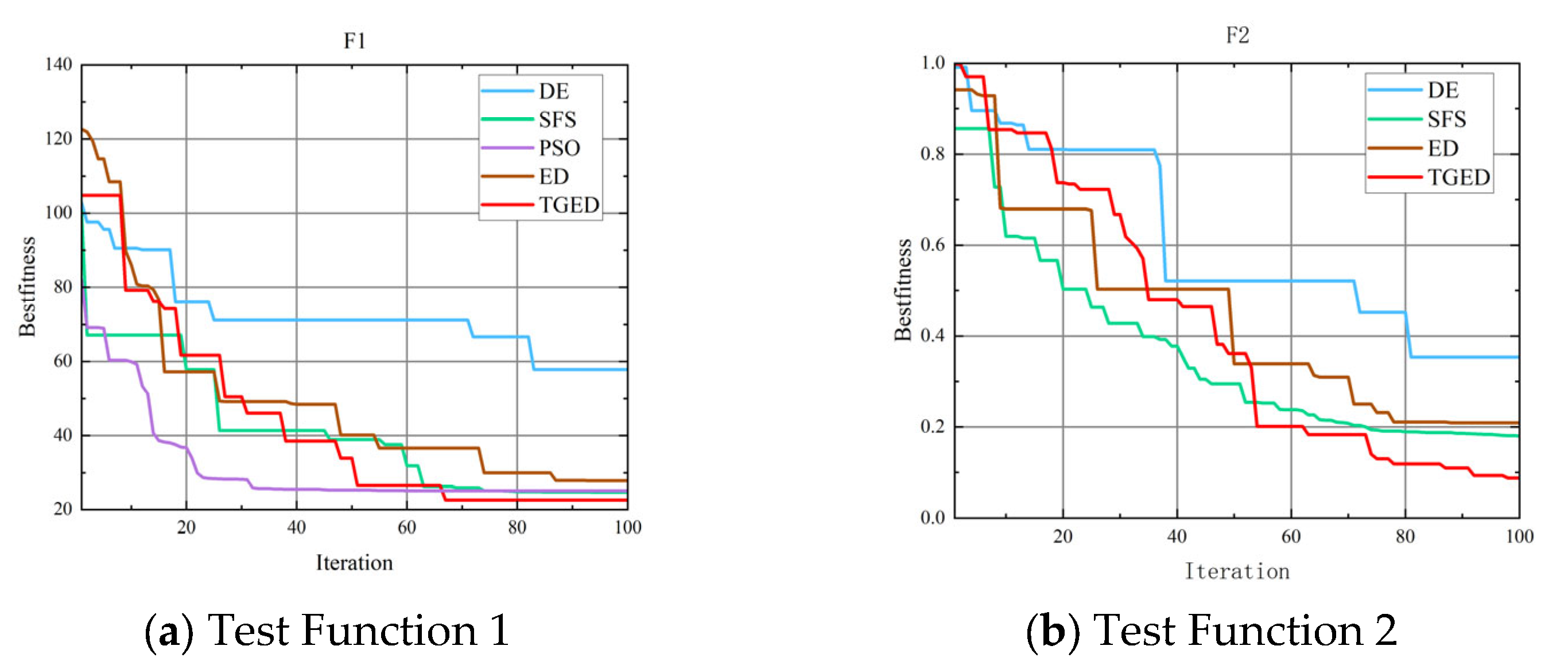
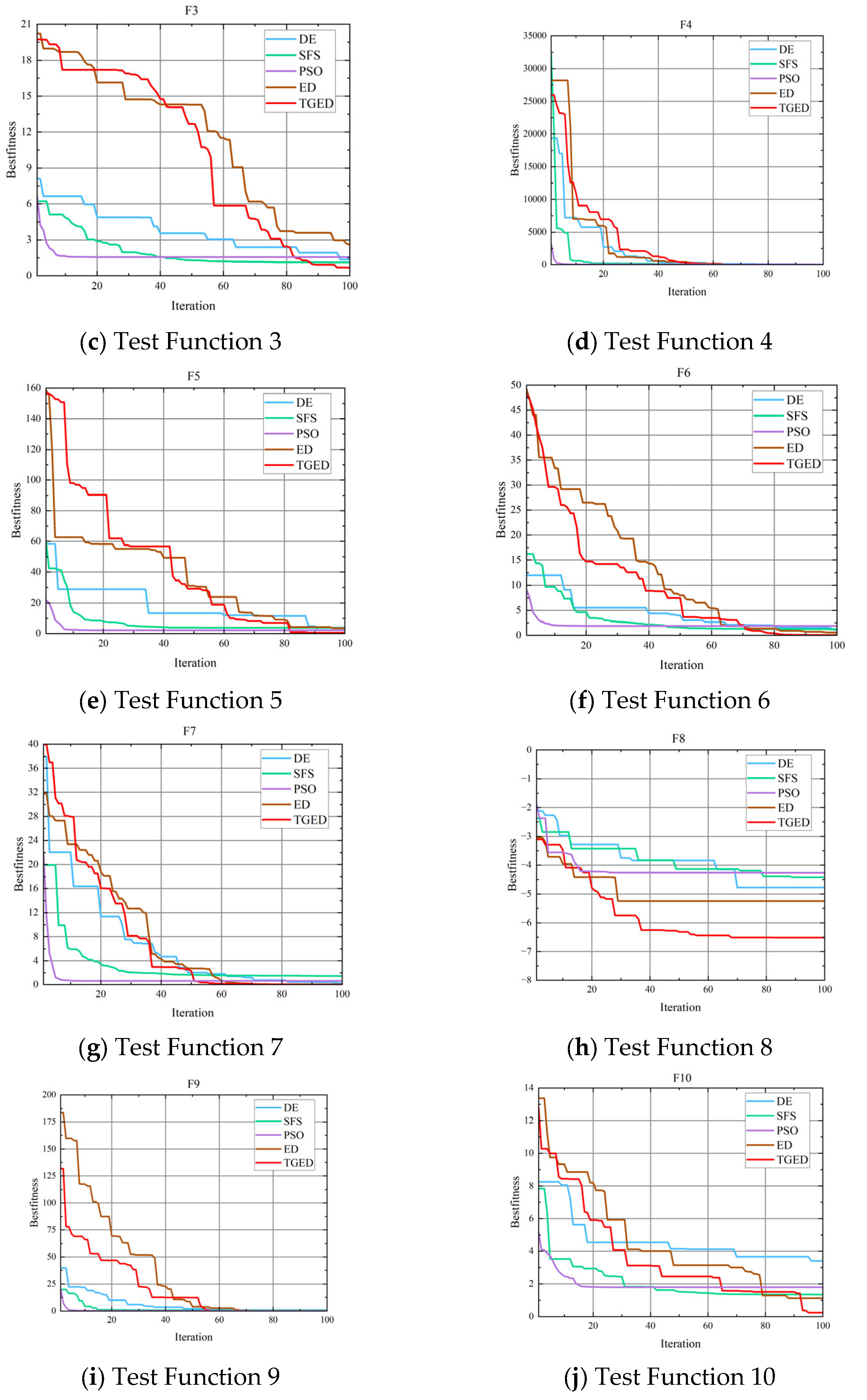
The optimization results and convergence curves are shown in Table 1 and Figure 2, respectively.
Based on the above comparison, it can be concluded that among the 10 commonly used benchmark functions, the TGED algorithm effectively avoids premature convergence during the optimization process. It achieves high solution accuracy and superior optimization performance compared to the unmodified original algorithm and other benchmark algorithms. This demonstrates that the improvements made to the ED algorithm are effective.
Although the results of the test functions partially demonstrate the superiority of the TGED algorithm, further validation is required through practical engineering problems to confirm the feasibility and efficiency of the improved algorithm in the optimization scheduling of hydro–wind–solar multi-energy complementarity.

5. Case Study

5.1. Engineering Background

This study focuses on a hydropower station and its integrated wind–solar resources, forming a hydro–wind–solar multi-energy complementary system, as well as the power grid for electricity transmission. The hydropower station is located on a major river in the southwestern region of China, with a normal reservoir elevation of 825 m and a total installed capacity of 16,000 MW. The installed capacities of wind power and photovoltaic power are 3470 MW and 1805 MW, respectively. The receiving power grids of the hydropower station cover two provincial-level grids, and in this study, 50% of the power output from the station is transmitted to one of these grids.

5.2. Analysis of Typical Days

This study uses four typical days as examples: 5 February 2022, as a dry season day with strong wind and weak solar energy (Typical Day 1); 4 August 2021, as a flood season day with strong solar and weak wind energy (Typical Day 2); 19 October 2021, as a flood season day with strong wind and weak solar energy (Typical Day 3); and 10 May 2022, as a dry season day with strong solar and weak wind energy (Typical Day 4). The scheduling period is set to one day (24 h) with a scheduling interval of 2 h, resulting in 12 scheduling periods. Simulated scheduling analyses are conducted under two scenarios: hydropower peak-shaving and hydro–wind–solar multi-energy complementary system peak-shaving. These analyses evaluate the regulation performance of the hydro–wind–solar complementary optimization scheduling model constructed in this study, based on the TGED algorithm, in balancing wind–solar output and grid load.
The inflow, initial, and final water levels for the scheduling period, as well as the upper and lower water level limits for typical days, are based on the actual operational data of the hydropower station, as shown in Table 2. The average daily loads for the four typical days are approximately 34,301 MW, 69,839 MW, 59,395 MW, and 61,789 MW, respectively. The case study employs the DE, SFS, ED, PSO, and TGED algorithms to solve the model, with algorithm parameters set as follows: the population size is set to 50, the individual dimension is set to 13, and the number of iterations is set to 100.
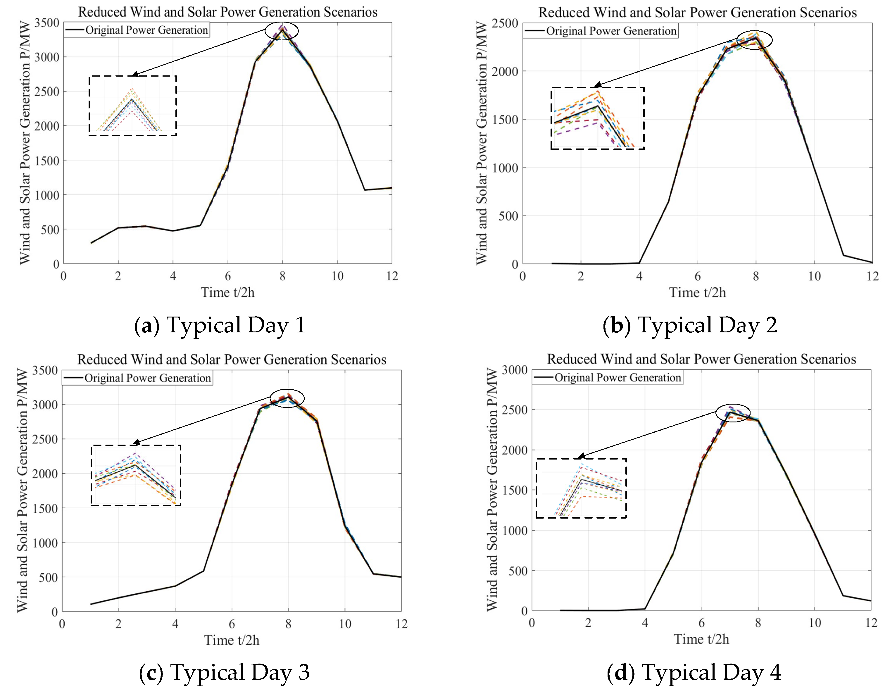
The wind and solar output scenarios for the four typical days are generated and reduced separately, with the typical scenario diagrams shown in Figure 3 below:
The ten wind–solar typical scenarios reduced for the four typical days passed the significance test with p > 0.05, based on the K-S test. This indicates that the Latin Hypercube Sampling and K-means clustering methods used in this study are reasonable.
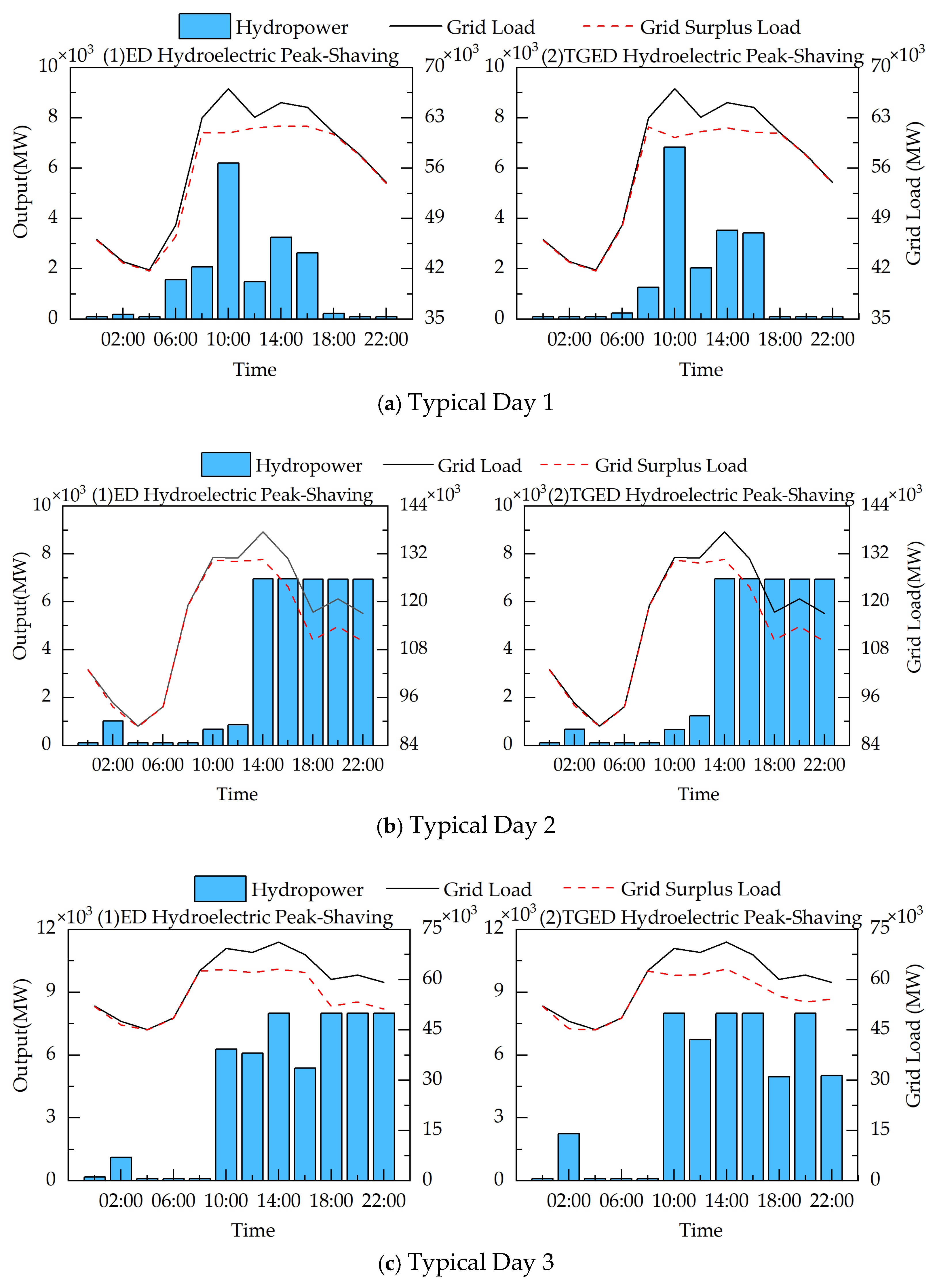
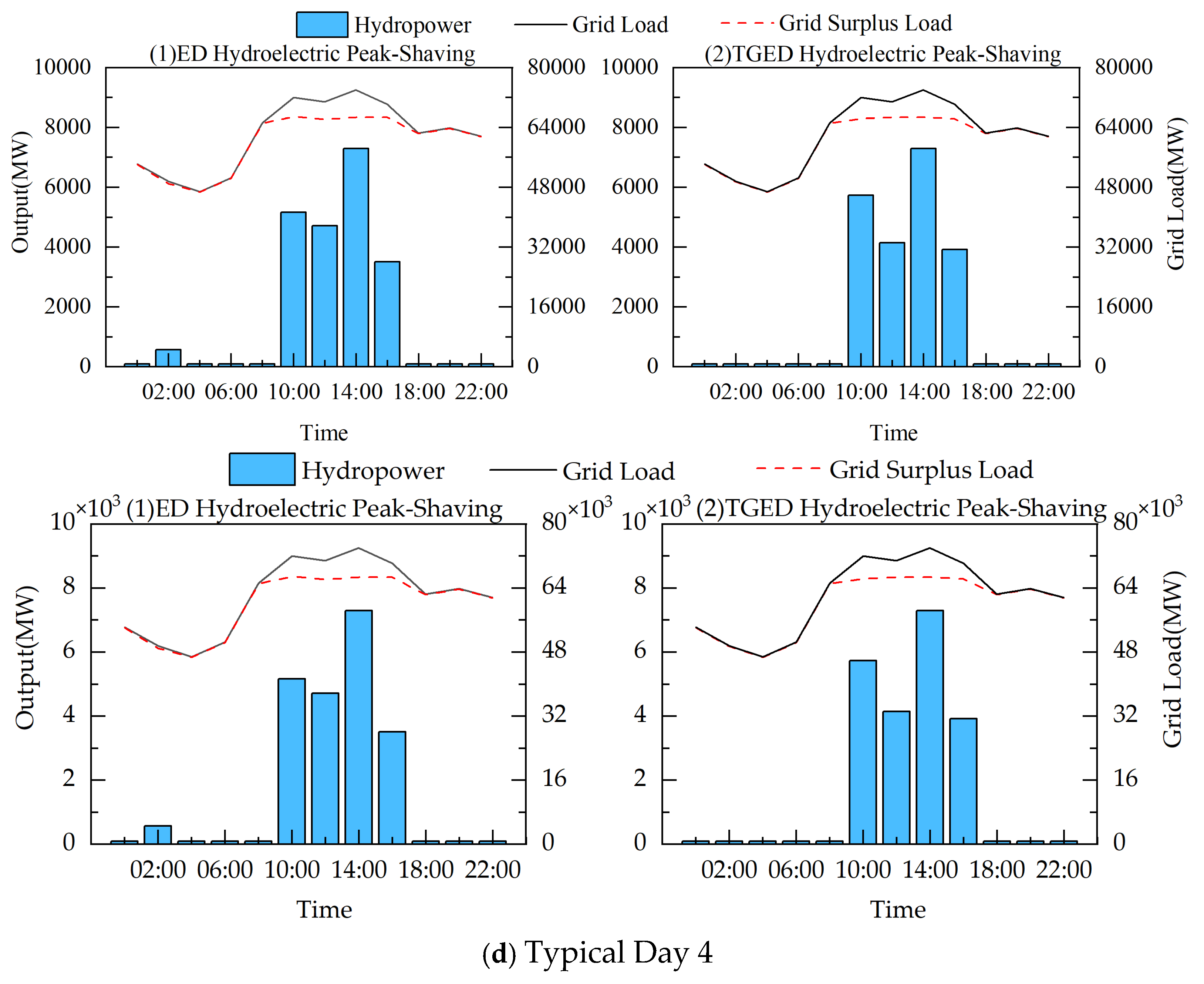
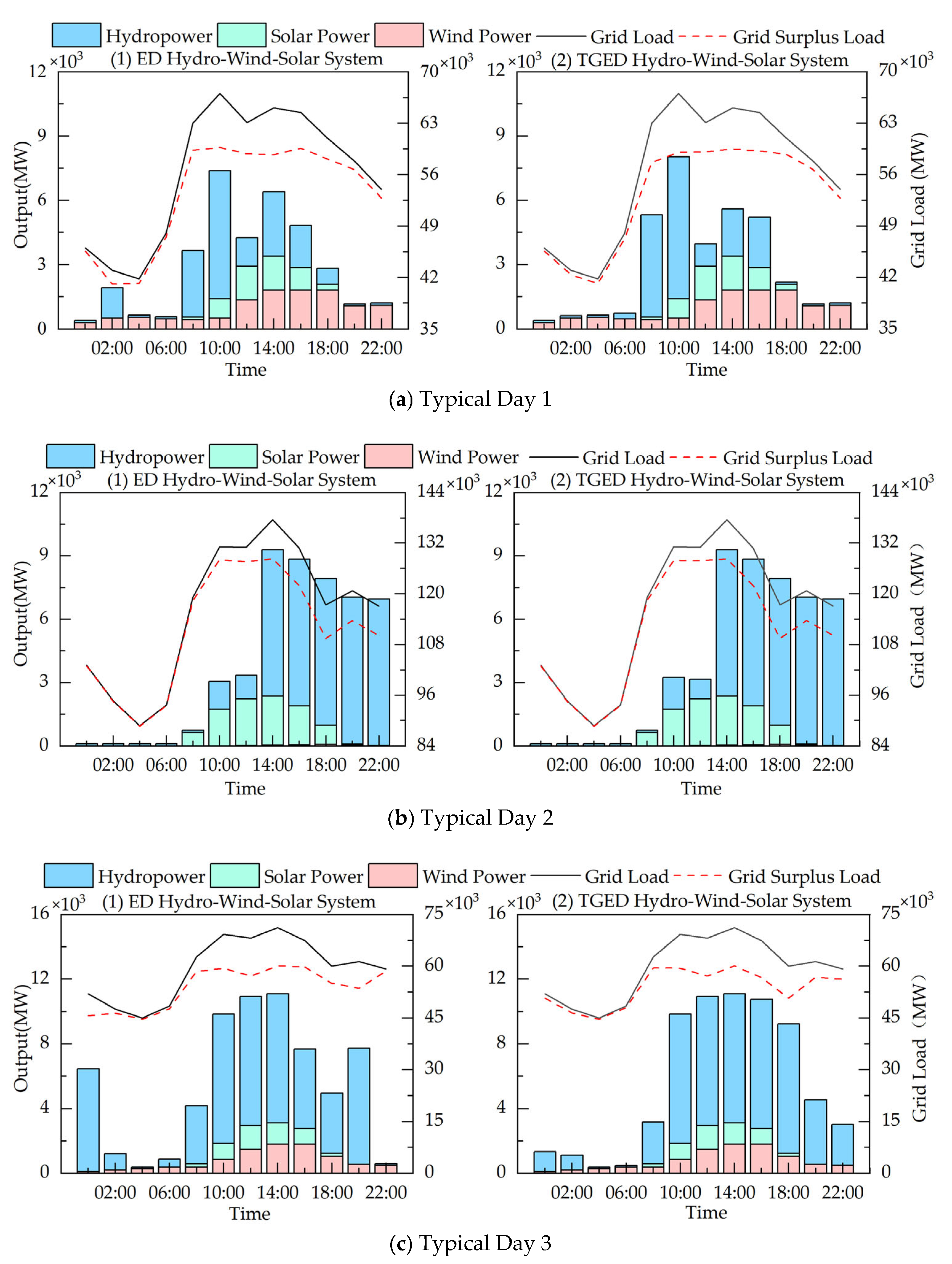
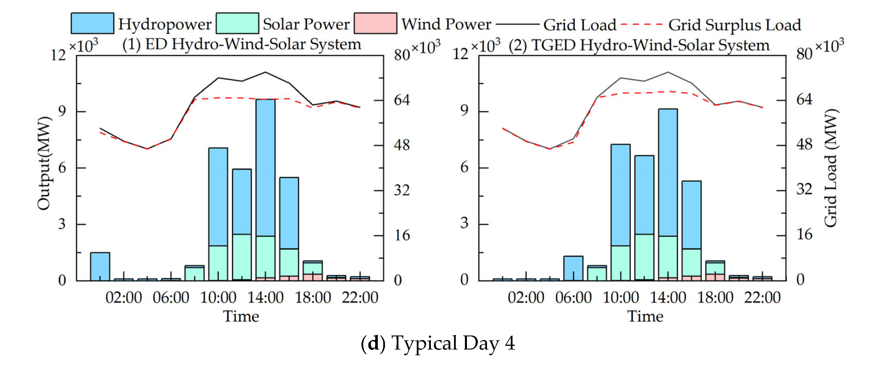
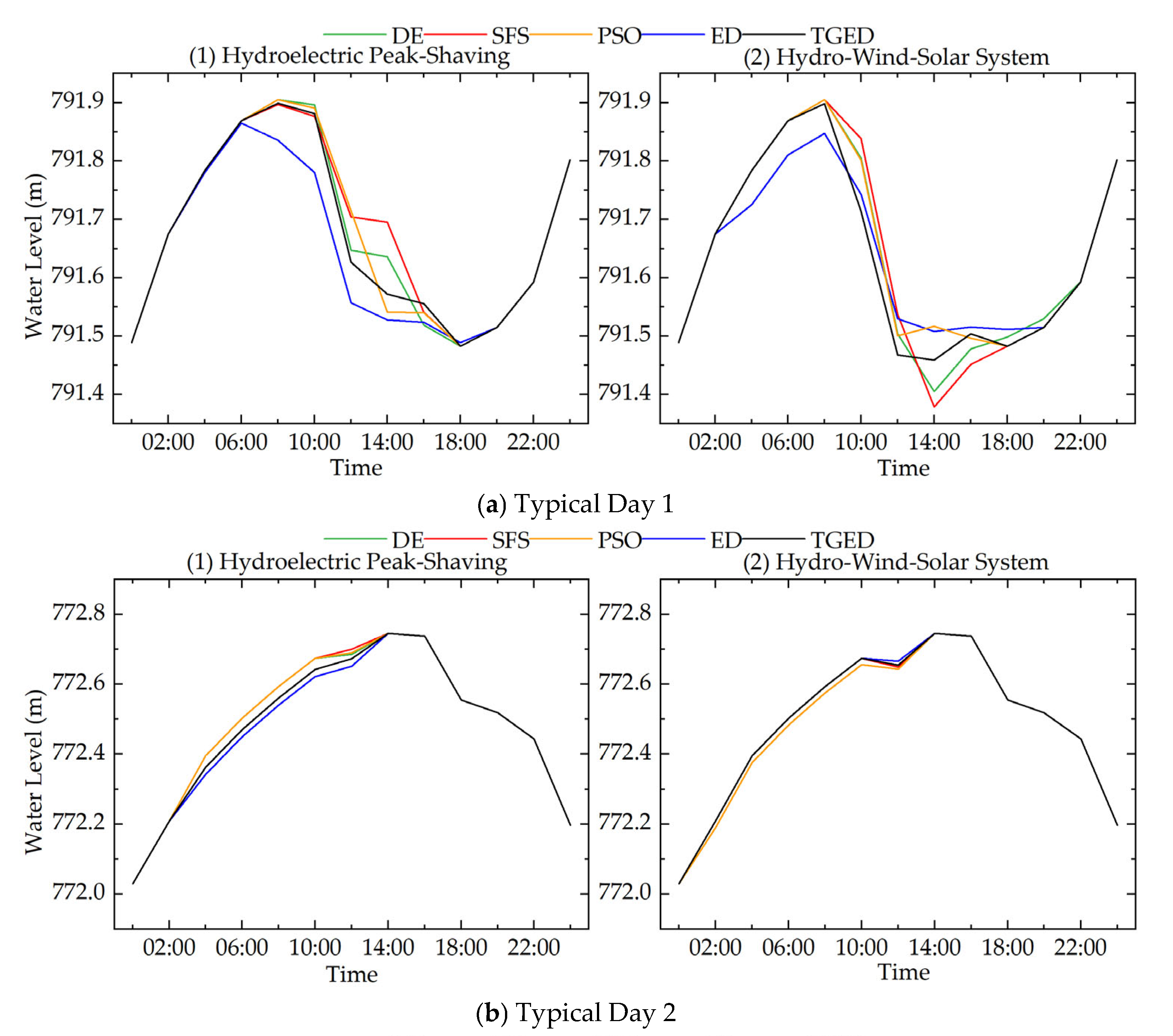
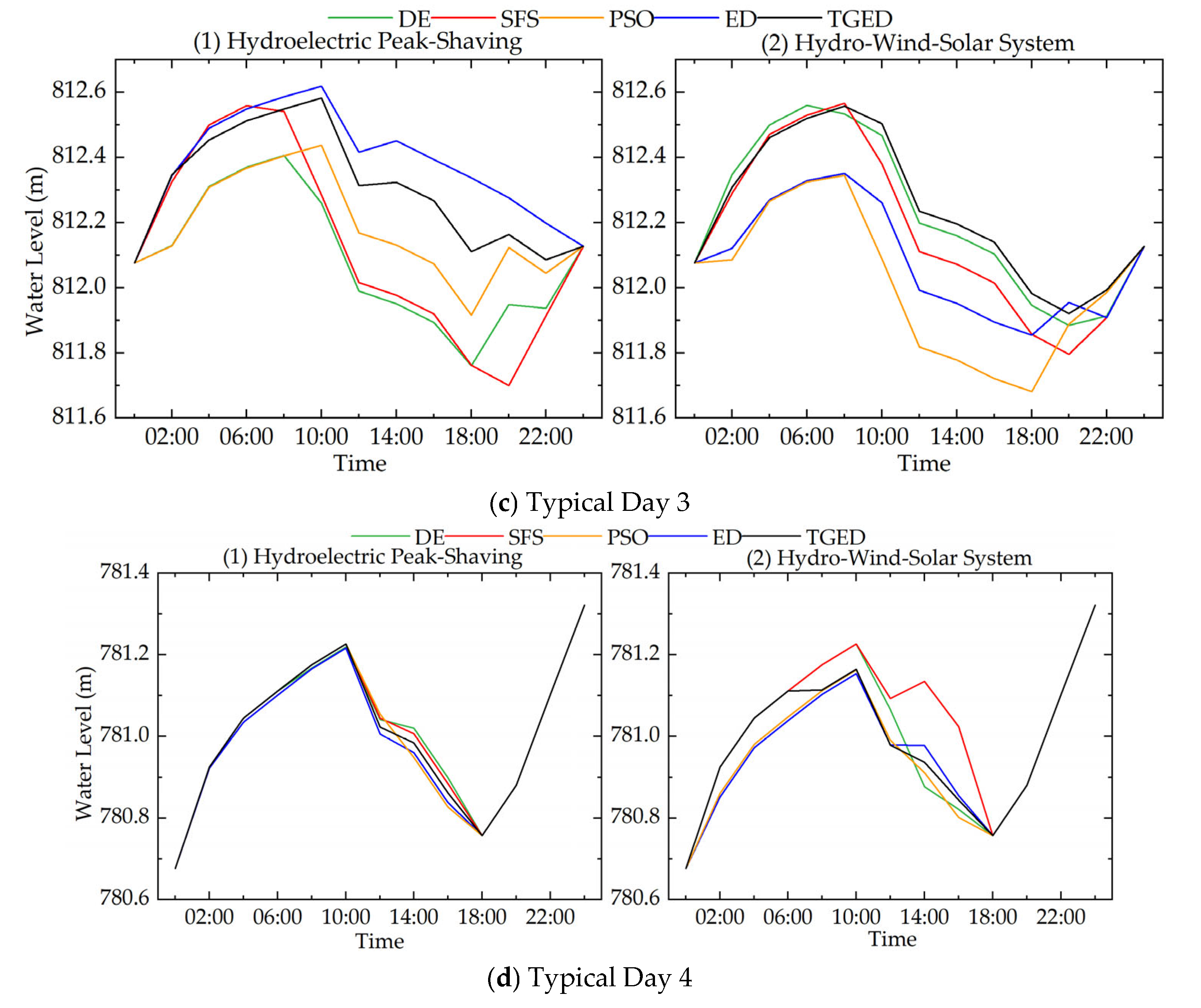
Figure 4, Figure 5 and Figure 6 below show the results of the hydroelectric peak-shaving operation and the hydro–wind–solar multi-energy complementary system operation for the four typical days:
By observing the results of the four typical days, it can be seen that, during the low-load periods, the output is reduced, water is stored, and the water level is increased. In contrast, during high-load periods, the water level is reduced, and the outflow is increased to enhance the output, effectively tracking the load variation process. From the residual load processes after hydroelectric peak-shaving and hydro–wind–solar complementary system peak-shaving, it is evident that, compared with the original load, the residual load after peak-shaving is smaller and the process is smoother, validating the effectiveness of the model constructed in this paper. Furthermore, whether for hydroelectric peak-shaving or hydro–wind–solar complementary system peak-shaving, the water level variation process obtained by the TGED algorithm has not exceeded the peak and valley values of the other three algorithms within a day, thus effectively avoiding rapid fluctuations in the reservoir water level in a short time.
Further comparisons of the peak-shaving performance between the TGED algorithm and four other algorithms are presented in Table 3. On the two typical dry season days (Day 1 and Day 4), both the hydro peak-shaving and hydro–wind–solar complementary system peak-shaving results optimized by the TGED algorithm yielded the smallest residual load peak–valley differences. On Typical Day 1, the hydro peak-shaving result achieved by the TGED algorithm was approximately 250 MW, 294 MW, 112 MW, and 163 MW lower than those of the DE, SFS, ED, and PSO algorithms, respectively, while the hydro–wind–solar complementary system peak-shaving result was reduced by approximately 633 MW, 862 MW, 286 MW, and 184 MW compared to DE, SFS, ED, and PSO, respectively. On Typical Day 4, the TGED algorithm’s hydro peak-shaving result was approximately 302 MW, 201 MW, 127 MW, and 111 MW lower than those of DE, SFS, ED, and PSO, respectively, and its hydro–wind–solar complementary system peak-shaving result was reduced by approximately 634 MW, 576 MW, 84 MW, and 734 MW, respectively. These results indicate that the application of the TGED algorithm not only enhances the model’s ability to adapt to the uncertainty of renewable energy outputs but also improves the quality of the optimization results. However, on the two typical flood season days, Day 2 and Day 3, the results obtained by all four algorithms were nearly the same. This suggests that when the flood season inflow is relatively large, the hydropower station plays a strong regulation role, and the optimization performance of the different algorithms is similar. On the other hand, for typical dry season days and flood season days with relatively small average inflows, the regulation range of hydropower output is limited, which places a greater demand on the optimization capability of the algorithms.
To further validate the peak-shaving performance of the TGED algorithm, this study calculates the mean square deviation (MSD) of the residual load for each typical day, based on the optimization objective of minimizing the residual load peak-to-valley difference. The results are presented in Table 4. Due to differences in optimization objectives, the TGED algorithm does not always yield the lowest MSD across all four typical days, indicating that, in some scenarios, optimizing solely for the minimum residual load peak-to-valley difference may adversely affect the overall stability of the residual load. Nevertheless, compared with other algorithms, the MSD of the residual load achieved by the TGED algorithm consistently remains within a reasonable and stable range without significant fluctuations. This result further demonstrates the comprehensive peak-shaving advantage of the TGED algorithm—it effectively reduces the peak-to-valley difference while maintaining good residual load stability, thereby providing reliable support for optimal scheduling in complex dispatch environments.
In addition, to evaluate the computational complexity and engineering feasibility of the TGED algorithm, this paper statistically analyzes the runtime of various algorithms under different peak-shaving schemes for typical days. The scheduling model was run on a uniform hardware configuration (Intel Core i7-12700KF 3.60 GHz processor, NVIDIA RTX 4070 GPU), and the runtimes of the TGED, ED, DE, SFS, and PSO algorithms were recorded to further compare their computational efficiency. Table 5 presents the actual runtimes of different algorithms under the hydropower peak-shaving and hydro–wind–solar complementary peak-shaving schemes. Since the hydro–wind–solar complementary system peak-shaving scheme takes into account the uncertainty of wind and solar output, its computational complexity is higher, leading to significantly increased runtimes compared with the standalone hydropower peak-shaving scheme. The TGED algorithm was improved based on the ED algorithm through an optimized initialization strategy and the introduction of a Gaussian random walk mechanism to enhance global search capability. However, these enhancements also increase the computational complexity to some extent, resulting in the TGED algorithm having a longer runtime than the ED algorithm under both peak-shaving schemes. Under the hydropower peak-shaving scheme, the TGED algorithm’s runtime is lower than that of the DE, SFS, and PSO algorithms, indicating that its improvement strategy maintains high computational efficiency while ensuring effective optimization performance. In the hydro–wind–solar complementary peak-shaving scheme, although the TGED algorithm’s runtime is slightly higher than that of the PSO algorithm, the difference is minimal and remains within a reasonable range. This demonstrates that despite the increased computational complexity, the enhancement in optimization quality provided by the TGED algorithm effectively compensates for the additional computational cost, thereby affirming its strong practical application value.
Under the influence of the volatility of wind and solar output, the stable operation of the grid load requires effective peak-shaving strategies to reduce the impact of wind and solar power on the system. The results for the four typical days show a decrease in both the residual load peak–valley difference and MSD after incorporating wind and solar power, indicating that the peak-shaving effectiveness of the hydro–wind–solar system is influenced by the degree of temporal overlap between the wind and solar output peak periods and the grid load peak periods. When the wind and solar output peak coincides with the load peak, it means that wind and solar power can provide more electricity during the peak period, thereby relieving the peak-shaving pressure on hydropower. Conversely, it increases the peak-shaving pressure on hydropower. The results of the four typical days validate the effectiveness of the hydro–wind–solar multi-energy complementary optimization scheduling model in adapting to wind and solar output uncertainty and balancing the grid load, offering valuable insights and reference for short-term intraday scheduling of hydro–wind–solar complementary systems.

6. Conclusions and Summary

In response to the challenges of grid peak-shaving caused by the uncertainty of wind and solar power generation, this paper utilizes Latin Hypercube Sampling (LHS) and K-means clustering to quantify the uncertainty of wind and solar output. With the objective of minimizing the system’s residual load peak–valley difference, we have developed a short-term optimization scheduling model for hydro–wind–solar multi-energy complementary systems based on the Improved Enterprise Development Optimization Algorithm (TGED). Through practical application in a certain hydropower station system, the effectiveness and superiority of the TGED algorithm in optimizing scheduling are verified. The main conclusions are as follows:
(1)
Effectiveness of the Improved Algorithm: This paper improves the Enterprise Development Optimization (ED) algorithm by combining chaotic initialization and Gaussian random walk with the standard algorithm. A new ED algorithm is proposed that enhances the solving accuracy and reduces the likelihood of falling into local optima. Preliminary validation through ten test functions shows that the TGED algorithm achieves high accuracy, faster convergence, and better optimization capabilities compared to other algorithms.
(2)
Peak-Shaving Performance Improvement: The TGED algorithm has optimized grid load peak-shaving across multiple typical day scenarios, demonstrating excellent optimization performance. Its adaptive update mechanism can rapidly respond to fluctuations in load and output, further smoothing the residual load process. Compared with the standard DE, SFS, PSO, and ED algorithms, the TGED algorithm exhibits superior peak-shaving results, further confirming its applicability in complex multi-energy scheduling environments.
(3)
Advantages of Hydro–Wind–Solar Complementarity: In multi-energy complementary operation, hydro–wind–solar complementarity uses the flexible regulation capability of hydropower to effectively suppress the fluctuations of wind and solar output, achieving a more stable grid load output, which facilitates efficient consumption of renewable energy. Typical day analysis shows that the hydro–wind–solar complementary optimization scheduling model based on TGED can effectively reduce the system’s load peak–valley difference under various meteorological conditions.
In summary, the findings of this study indicate that the TGED algorithm can effectively support the peak-shaving scheduling of hydro–wind–solar multi-energy complementary systems. It exhibits robust regulation capabilities in complex scenarios characterized by the large-scale integration of wind and solar power into the grid, thereby offering superior scheduling solutions for clean energy consumption in challenging environments. This study focused solely on optimizing a single objective function (the residual load peak-to-valley difference), primarily because the TGED algorithm is currently tailored for solving single-objective optimization problems. In the future, we plan to further refine the model by incorporating a multi-objective optimization framework that considers multiple factors such as total power generation, operation and maintenance costs, and environmental impacts, in order to achieve a more comprehensive and efficient scheduling strategy. Additionally, we will explore the integration of other intelligent optimization methods or develop more efficient hybrid strategies to further enhance the algorithm’s efficiency and adaptability.

Author Contributions

Conceptualization, G.Z. and C.Y.; methodology, G.Z.; software, H.H.; validation, C.Y. and Y.Y.; formal analysis, H.H.; investigation, L.Z.; resources, L.Z.; data curation, H.H.; writing—original draft preparation, G.Z.; writing—review and editing, G.Z. and C.Y.; visualization, Y.Y.; supervision, C.Y. and L.M.; project administration, C.Y.; funding acquisition, L.M. All authors have read and agreed to the published version of the manuscript.

Funding

This research was funded by China Yangtze Power Co., Ltd., contract number Z532302054.

Institutional Review Board Statement

Not applicable.

Informed Consent Statement

Not applicable.

Data Availability Statement

Data unavailable due to privacy restriction.

Conflicts of Interest

Guohan Zhao and Linfeng Zou are from the China Three Gorges Jinsha River Yunchuan Hydropower Development Co., Ltd. The remaining authors declare that the research was conducted in the absence of any commercial or financial relationships that could be construed as a potential conflict of interest.

Abbreviations

The following abbreviations are used in this manuscript:
TGEDTent–Gaussian Enterprise Development Optimization
EDEnterprise Development Optimization
DEDifferential Evolution
SFSStochastic Fractal Search
PSOLinear dichroism

References

  1. Yang, G.; Kong, D.; He, X.; Yu, X.; Jiang, K. Prediction of hydrogen leakage location and intensity in hydrogen refueling stations based on deep learning. Int. J. Hydrogen Energy 2024, 68, 209–220. [Google Scholar] [CrossRef]
  2. Yogeswari, M.K.; Dharmalingam, K.; Mullai, P. Implementation of artificial neural network model for continuous hydrogen production using confectionery wastewater. J. Environ. Manag. 2019, 252, 8. [Google Scholar] [CrossRef] [PubMed]
  3. Zhao, X.; Ma, X.; Chen, B.; Shang, Y.; Song, M. Challenges toward carbon neutrality in china: Strategies and countermeasures. Resour. Conserv. Recycl. 2022, 176, 9. [Google Scholar] [CrossRef]
  4. Yuan, K.; Zhang, T.; Xie, X.; Du, S.; Xue, X.; Abdul-Manan, A.F.N.; Huang, Z. Exploration of low-cost green transition opportunities for china’s power system under dual carbon goals. J. Clean. Prod. 2023, 414, 15. [Google Scholar] [CrossRef]
  5. Babay, M.; Adar, M.; Chebak, A.; Mabrouki, M. Forecasting green hydrogen production: An assessment of renewable energy systems using deep learning and statistical methods. Fuel 2025, 381, 31. [Google Scholar] [CrossRef]
  6. Chen, Y.; Liu, J.; Feng, L. Transient analysis of a green hydrogen production and storage system using alkaline electrolyzer. Fuel 2022, 324, 10. [Google Scholar] [CrossRef]
  7. Qing, X.; Niu, Y. Hourly day-ahead solar irradiance prediction using weather forecasts by LSTM. Energy 2018, 148, 461–468. [Google Scholar] [CrossRef]
  8. Zhang, Z.; Qin, H.; Li, J.; Liu, Y.; Yao, L.; Wang, Y.; Wang, C.; Pei, S.; Zhou, J. Short-term optimal operation of wind-solar-hydro hybrid system considering uncertainties. Energy Convers. Manag. 2020, 205, 16. [Google Scholar] [CrossRef]
  9. Babay, M.; Adar, M.; Chebak, A.; Mabrouki, M. Comparative sustainability analysis of serpentine flow-field and straight channel PEM fuel cell designs. Int. J. Syst. Assur. Eng. Manag. 2024, 15, 3954–3970. [Google Scholar] [CrossRef]
  10. Wei, H.; Zhang, H.X.; Yu, D.; Wang, Y.T.; Ling, D.; Ming, X. Short-term optimal operation of hydro-wind-solar hybrid system with improved generative adversarial networks. Appl. Energy 2019, 250, 389–403. [Google Scholar] [CrossRef]
  11. Liu, Z.; Mo, L.; Lou, S.; Zhu, Y.; Liu, T. An ecology-oriented single—Multi-objective optimal operation modeling and decision-making method in the case of the ganjiang river. Water 2024, 16, 970. [Google Scholar] [CrossRef]
  12. Fu, K.; Sun, X.; Chen, K.; Mo, L.; Xiao, W.; Liu, S. Monthly runoff prediction based on stochastic weighted averaging-improved stacking ensemble model. Water 2024, 16, 3580. [Google Scholar] [CrossRef]
  13. Hart, E.K.; Jacobson, M.Z. A monte carlo approach to generator portfolio planning and carbon emissions assessments of systems with large penetrations of variable renewables. Renew. Energy 2011, 36, 2278–2286. [Google Scholar] [CrossRef]
  14. Zhang, H.; Lu, Z.; Hu, W.; Wang, Y.; Dong, L.; Zhang, J. Coordinated optimal operation of hydro-wind-solar integrated systems. Appl. Energy 2019, 242, 883–896. [Google Scholar] [CrossRef]
  15. Yu, H.; Chung, C.Y.; Yong, K.P.; Lee, H.W.; Zhang, J.H. Probabilistic load flow evaluation with hybrid latin hypercube—Sampling and cholesky decomposition. IEEE Trans. Power Syst. 2009, 24, 661–667. [Google Scholar] [CrossRef]
  16. Heitsch, H.; Römisch, W. Scenario reduction algorithms in stochastic programming. Comput. Optim. Appl. 2003, 24, 187–206. [Google Scholar] [CrossRef]
  17. Wang, Y.; Liu, Y.; Kirschen, D.S. Scenario reduction with submodular optimization. IEEE Trans. Power Syst. 2017, 32, 2479–2480. [Google Scholar] [CrossRef]
  18. Dupacová, J.; Gröwe-Kuska, N.; Römisch, W. Scenario reduction in stochastic programming: An approach using probability metrics. Math. Program. 2003, 95, 493–511. [Google Scholar] [CrossRef]
  19. Lv, S.; Wang, H.; Meng, X.; Yang, C.; Wang, M. Optimal capacity configuration model of power-to-gas equipment in wind-solar sustainable energy systems based on a novel spatiotemporal clustering algorithm: A pathway towards sustainable development. Renew. Energy 2022, 201, 240–255. [Google Scholar] [CrossRef]
  20. Li, F.; Chen, S.; Ju, C.; Zhang, X.; Ma, G.; Huang, W. Research on short-term joint optimization scheduling strategy for hydro-wind-solar hybrid systems considering uncertainty in renewable energy generation. Energy Strateg. Rev. 2023, 50, 17. [Google Scholar] [CrossRef]
  21. Jiang, W.; Liu, Y.; Fang, G.; Ding, Z. Research on short-term optimal scheduling of hydro-wind-solar multi-energy power system based on deep reinforcement learning. J. Clean. Prod. 2023, 385, 12. [Google Scholar] [CrossRef]
  22. Wang, X.; Chang, J.; Meng, X.; Wang, Y. Hydro-thermal-wind-photovoltaic coordinated operation considering the comprehensive utilization of reservoirs. Energy Convers. Manag. 2019, 198, 15. [Google Scholar] [CrossRef]
  23. Zhang, X.; Wang, M.; Jia, T.; Ma, X.; Song, Q.; Zhou, Q.; Yang, X.; Liu, J.; Guo, A. A heat-resistant glass-modified multi-component phosphate adhesive for repair and connection of superalloy in extreme environment. J. Alloys Compd. 2018, 745, 868–873. [Google Scholar] [CrossRef]
  24. Jin, X.; Liu, B.; Liao, S.; Cheng, C.; Li, G.; Liu, L. Impacts of different wind and solar power penetrations on cascade hydroplants operation. Renew. Energy 2022, 182, 227–244. [Google Scholar] [CrossRef]
  25. Huang, S.J. Enhancement of hydroelectric generation scheduling using ant colony system based optimization approaches. IEEE Trans. Energy Convers. 2001, 16, 296–301. [Google Scholar] [CrossRef]
  26. Truong, D.; Chou, J. Metaheuristic algorithm inspired by enterprise development for global optimization and structural engineering problems with frequency constraints. Eng. Struct. 2024, 318, 25. [Google Scholar] [CrossRef]
  27. Daneshvar, M.; Mohammadi-Ivatloo, B.; Zare, K. Two-stage optimal robust scheduling of hybrid energy system considering the demand response programs. J. Clean. Prod. 2020, 248, 13. [Google Scholar] [CrossRef]
  28. Mazidi, M.; Zakariazadeh, A.; Jadid, S.; Siano, P. Integrated scheduling of renewable generation and demand response programs in a microgrid. Energy Convers. Manag. 2014, 86, 1118–1127. [Google Scholar] [CrossRef]
  29. Shu, Z.; Jirutitijaroen, P. Latin hypercube sampling techniques for power systems reliability analysis with renewable energy sources. IEEE Trans. Power Syst. 2011, 26, 2066–2073. [Google Scholar] [CrossRef]
  30. Lu, L.; Yuan, W.; Su, C.; Wang, P.; Cheng, C.; Yan, D.; Wu, Z. Optimization model for the short-term joint operation of a grid-connected wind-photovoltaic-hydro hybrid energy system with cascade hydropower plants. Energy Convers. Manag. 2021, 236, 12. [Google Scholar] [CrossRef]
  31. Shatrevich, V. Industrial structures as competitive factor in organization development. In Proceedings of the 2nd International Scientific Conference—Contemporary Issues in Business, Management and Education, Vienna, Austria, 13–14 May 2013; Volume 110, pp. 871–878. [Google Scholar] [CrossRef]
  32. Glasauer, C. The PREVENT-model: Human and organizational factors fostering engineering of safe and secure robotic systems. J. Syst. Softw. 2023, 195, 17. [Google Scholar] [CrossRef]
  33. Chen, M.S.; Gu, Y.L. The mechanism and measures of adjustment of industrial organization structure: The perspective of energy saving and emission reduction. In Proceedings of the 2010 International Conference on Energy, Environment and Development (Iceed2010), Kuala Lumpur, Malaysia, 8–9 December 2010; Volume 5, pp. 2562–2567. [Google Scholar] [CrossRef]
  34. Shao, S.; Peng, Y.; He, C.; Du, Y. Efficient path planning for UAV formation via comprehensively improved particle swarm optimization. ISA Trans. 2020, 97, 415–430. [Google Scholar] [CrossRef] [PubMed]
  35. Xu, A.; Mo, L.; Wang, Q. Research on operation mode of the yalong river cascade reservoirs based on improved stochastic fractal search algorithm. Energies 2022, 15, 7779. [Google Scholar] [CrossRef]
  36. Qin, A.K.; Suganthan, P.N. Self-adaptive differential evolution algorithm for numerical optimization. In Proceedings of the 2005 IEEE Congress on Evolutionary Computation, Proceedings, Scotland, UK, 2–5 September 2005; Volumes 1–3, pp. 1785–1791. [Google Scholar] [CrossRef]
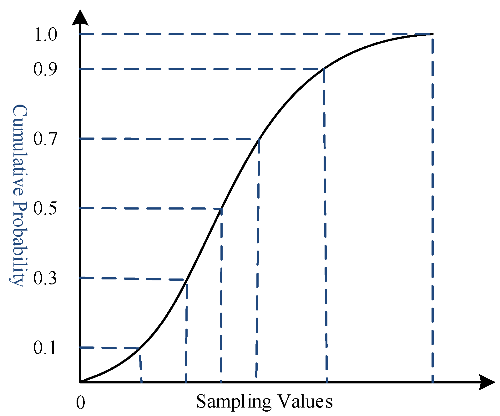
Figure 1. Schematic of Latin Hypercube Sampling.
Sustainability 17 02691 g001
Figure 2. Convergence Curves of Ten Test Functions for Different Algorithms.
Sustainability 17 02691 g002aSustainability 17 02691 g002b
Figure 3. Wind–Solar Typical Scenarios for Typical Days.
Sustainability 17 02691 g003
Figure 4. Hydroelectric Peak-Shaving Operation Results for Typical Days.
Sustainability 17 02691 g004aSustainability 17 02691 g004b
Figure 5. Hydro–Wind–Solar Complementary System Operation Results for Typical Days.
Sustainability 17 02691 g005aSustainability 17 02691 g005b
Figure 6. Water Level Variation Process for Typical Days.
Sustainability 17 02691 g006aSustainability 17 02691 g006b
Table 1. Computation Results of Test Functions for Different Algorithms.
No.TypeTest Function x i Value RangeOptimal Value
TGEDEDDESFSPSO
1Multimodal f 1 ( x ) [−5.12,5.12]22.56127.82957.79024.68225.095
2Multimodal f 2 ( x ) [−6,6]0.0880.2090.3530.1800.229
3Multimodal f 3 ( x ) [−32.768,32.768]0.6662.6121.3591.1241.560
4Unimodal f 4 ( x ) [−5,5]9.37610.12743.58732.29836.535
5Multimodal f 5 ( x ) [−5,10]0.5553.5332.2033.7422.157
6Unimodal f 6 ( x ) [−10,10]0.0500.5831.1091.2351.884
7Unimodal f 7 ( x ) [−5,5]0.0010.0350.2651.4530.623
8Multimodal f 8 ( x ) [0,π]−6.512−5.246−4.775−4.418−4.263
9Multimodal f 9 ( x ) [−10,10]00.0390.1690.8230.272
10Multimodal f 10 ( x ) [−10,10]0.2461.1263.4111.3481.797
Table 2. Parameter Settings for Typical Days of the Hydropower Station.
Typical DayTypical Day 1 (5 February 2022)Typical Day 2 (4 August 2021)Typical Day 3 (19 October 2021)Typical Day 4 (10 May 2022)
Initial Water Level (m)791.489772.029812.076780.676
Final Water Level (m)791.802772.196812.127781.322
Average Inflow Rate (m3/s)2229.4504175.6674392.7863279.863
Upper Water Level Limit (m)794.489775.029815.076783.676
Lower Water Level Limit (m)789.489770.029810.076778.676
Table 3. Calculation Results of Residual Load Peak–Valley Difference for Typical Days.
Peak-Shaving SchemeAlgorithmTypical Day 1 (5 February 2022)Typical Day 2 (4 August 2021)Typical Day 3 (19 October 2021)Typical Day 4 (10 May 2022)
Hydro Peak-Shaving (MW)DE20,305.05641,933.28818,253.65720,312.989
SFS20,348.81441,933.28118,253.65920,211.558
PSO20,218.02841,933.28818,253.65720,125.865
ED20,166.45341,933.27318,253.65720,137.728
TGED20,054.82541,933.27318,253.65720,010.942
Hydro–Wind–Solar Peak-Shaving (MW)DE18,986.45139,591.00415,434.33618,787.417
SFS19,214.94339,591.00415,434.33218,730.139
PSO18,537.14639,591.00415,434.33218,887.543
ED18,639.18239,591.00415,434.33518,237.425
TGED18,353.09439,591.00415,434.33218,153.789
Table 4. Residual Load Mean Square Deviation Calculation Results for Typical Days.
Peak-Shaving SchemeAlgorithmTypical Day 1 (5 February 2022)Typical Day 2 (4 August 2021)Typical Day 3 (19 October 2021)Typical Day 4 (10 May 2022)
Hydro Peak-Shaving (MW)DE7586.22114,296.9146270.7197296.032
SFS7621.97314,298.9376166.4877264.329
PSO7594.92414,297.3506543.3287268.999
ED7790.16314,486.5556709.9617353.426
TGED7581.35014,413.5516286.2717262.861
Hydro–Wind–Solar Peak-Shaving (MW)DE6872.58914,062.3955410.8256644.506
SFS6911.99313,506.2075131.8456648.868
PSO6839.79713,556.1595806.6276759.444
ED7086.41213,506.0645835.2966770.382
TGED6853.25313,505.9335218.5726794.697
Table 5. Comparison of Algorithm Runtimes in the Scheduling Model.
Peak-Shaving SchemeRuntime (min)
TGEDEDDESFSPSO
Hydro Peak-Shaving0.0230.0160.0260.0280.027
Hydro–Wind–Solar Peak-Shaving12.33011.54112.89813.30212.248
Disclaimer/Publisher’s Note: The statements, opinions and data contained in all publications are solely those of the individual author(s) and contributor(s) and not of MDPI and/or the editor(s). MDPI and/or the editor(s) disclaim responsibility for any injury to people or property resulting from any ideas, methods, instructions or products referred to in the content.