Fisheries Sustainability Eroded by Lost Catch Proportionality in a Coral Reef Seascape

Abstract

Coral reef and their ecological services of food production and shoreline protection are threatened by unsustainable use. To better understand their status, multiple approaches to estimating fisheries sustainability were compared, namely fisheries-independent stock biomass and recovery rates, fisheries-dependent landed catches, balanced harvest and gear use metrics, and fish length measurements. A community biomass recovery was established over a 45-year no-fishing stock recovery time series from seven fisheries reserves and compared to catch- and length-based estimates of sustainability. The logistic production rates (r = 0.09 ± 0.06 95% confidence interval (CI)) and maximum equilibrium total biomass (~150 ± 30 tons/km²) indicated a broad range of potential maximum sustainable yields, with a likely range of 1.1 to 3.9 (95% CI; mean = 3.8) tons/km²/year. In contrast, the mean annual linear biomass growth rates in reserves were lower but less variable than logistic surplus production estimates, ranging from 2.1 to 3.5 (mean = 2.8 tons/km²/year). Realized catches at landing sites were lower still, ranging from 1.43 to 1.52 (mean = 1.48 ± 0.2 tons/km²/y). Differences between production estimates and capture were largely attributable to changes in taxonomic composition and an imbalance in the estimated proportionality of production potential versus actual capture rates. Lost potential capture was likely due to differences in the vulnerability of taxa to fishing and a lack of compensatory increased production among fishing-resistant taxa. Large proportional losses of catch were measured among snappers, unicorn fish, sweetlips, goatfish, and soldierfish, while smaller proportional gains in the catch samples were found among resident herbivorous rabbitfish, parrotfish, and groupers. Many of these declining taxa have vulnerable schooling life histories that are likely to require special habitat and reserve characteristics. Evaluations of sustainability from length measurements found 17 or 7% of total and 12% of caught species had sample sizes minimally sufficient for evaluation (>30 individuals from 413 catches, 2284 captured individuals composed of 144 species) of length and spawning metrics of sustainability. Seven of these species met length-based and three met spawning potential ratio thresholds for sustainability. Consequently, length-based evaluations had poor species coverage and therefore we were unable to evaluate the sustainability of the larger fish community. Recommendations for future research include a better understanding of the consequences of variability in spillover and proportionality of production potential for sustainability. Management recommendations are to focus management on the recovery of species abundant in unfished locations but not contributing to fisheries yield.

1. Introduction

Sustainable fisheries are one of the major challenges facing humanity [1]. In the tropics, limited reliable stock and yield information have challenged efforts to sustainably manage fisheries [2]. Most tropical fisheries assessments are based on landed fish weights and body length information [3,4,5]. Fisheries-independent measurements and analytical methods required to validate catch status in species-diverse fisheries can be expensive and seldom completed [6]. The common usage of expedient sustainability metrics can therefore potentially hinder robust evaluations understanding of stock status in tropical fisheries. For example, long-standing disagreements between the recommendations arising from catch and stock assessments have persisted [7]. Consequently, understanding how common fisheries status metrics influence desired levels of fishing effort and mortality is needed.

There are a variety of stock and catch production estimate methodologies. Moreover, measures reliant on pooled communities or individual species and stocks and catch foci have several consequences. In species-diverse coral reef fisheries, many species contribute small amounts to the larger community biomass and yield. Therefore, a mix of sustainably and unsustainably fished species is likely present when community biomass is evaluated [8]. Careful consideration of sampling, cost–benefit, and analysis of sustainability metrics are therefore needed to articulate fisheries status among the various biomass, production, size-at-capture, and reproductive metrics [9].

Community production may vary depending on the selective measure and capture of species relative to the species and community production rates. Balancing fisheries production and capture rates of species, or “balanced harvesting”, is therefore considered a management goal to maximize fisheries production [10]. Because production estimates of all species are seldom available, most balanced harvest evaluations use proxies, such as body lengths and theoretical or empirical body size spectrum data [11]. The gear-as-niche capture model is a related concept that promotes proportionality in gear use The model recommends reducing or eliminating dominant or competitive gear that extirpates large-bodied species, which subsequently favors the capture of resilient small, productive, and suboptimal sized individuals and species [12].

Selected species-level metrics of sustainability, such as size and reproduction status, may correspond poorly with the more holistic community status metrics of biomass and production [13]. Length and life history metrics used to evaluate species sustainability frequently fail to measure the entire community or to produce a holistic ecosystem measures of sustainability. For example, length-based metrics, such as size at reproduction and spawning potential ratio (SPR) may only be possible for a limited number of species. Few species have locally validated spawning rates and obtaining minimum required sample sizes for evaluation may be hindered by limited budgets.

The studied fisheries ecosystem was within a coral reef island environment of southern Kenya and northern Tanzania, a uniquely large lagoonal environment and species assemblage [14] (Figure 1). East African fisheries are largely reported to have high variability in management effectiveness and to be overfished based on various ecological and fish assessments [15,16]. Benchmarks for determining this status are frequently fish biomass evaluations comparing fished reefs under different management systems with numerous effective high-compliance fisheries closures that range in age from a few years to 45 years of no fishing [15]. Differences in fish biomass among low compliance and community closures are evident in terms of the rate of recovery and final biomass equilibrium [15]. The fish production and capture status context have, however, not been disarticulated to fully evaluate the proposed imbalance between production and capture rates, especially the meso-scale variability in production and capture among different geographies; for example, the leeward large lagoonal system behind the inhabited islands of Pemba, Zanzibar, and Mafia. Here, we assess the status of this lagoon by comparing several methods used to estimate sustainability.

Catch landings and recovery of stocks were evaluated in a network of variable age and management fisheries closures. The biomass of fished locations and in closures with different times since closure provided a 45-year time series of biomass recovery known as a space-for-time substitution. The capture, biomass, and recovery rates provided estimates of sustainable production using a variety of methods. These included fisheries-independent stock biomass and recovery rates and fisheries-dependent landed catches, the balance or proportionality between stocks in the closures and in the catch, and fish length and reproduction status metrics. The comparison of methods was expected to reveal potential biases, convergences, blind spots, and cost–benefit considerations relevant to collecting common metrics used to estimate reef fisheries sustainability.

A series of related methodological questions were asked. Specifically, if (1) recovery rates in fisheries reserves could be used to accurately estimate production rates of the fisheries, (2) if fishable production estimates from long-term recovery in reserves would match shorter-term (i.e., annual) stock and catch production estimates, (3) if taxonomic composition and production rates (fisheries yields) of key taxa accurately reflected fishable production estimates, (4) if proportionality in taxonomic composition in the catch was maintained between the landed catch and an older unfished reserve, and (5) if common length and spawning metrics were useful measures of fisheries sustainability for modest sampling effort and costs.

2. Materials and Methods

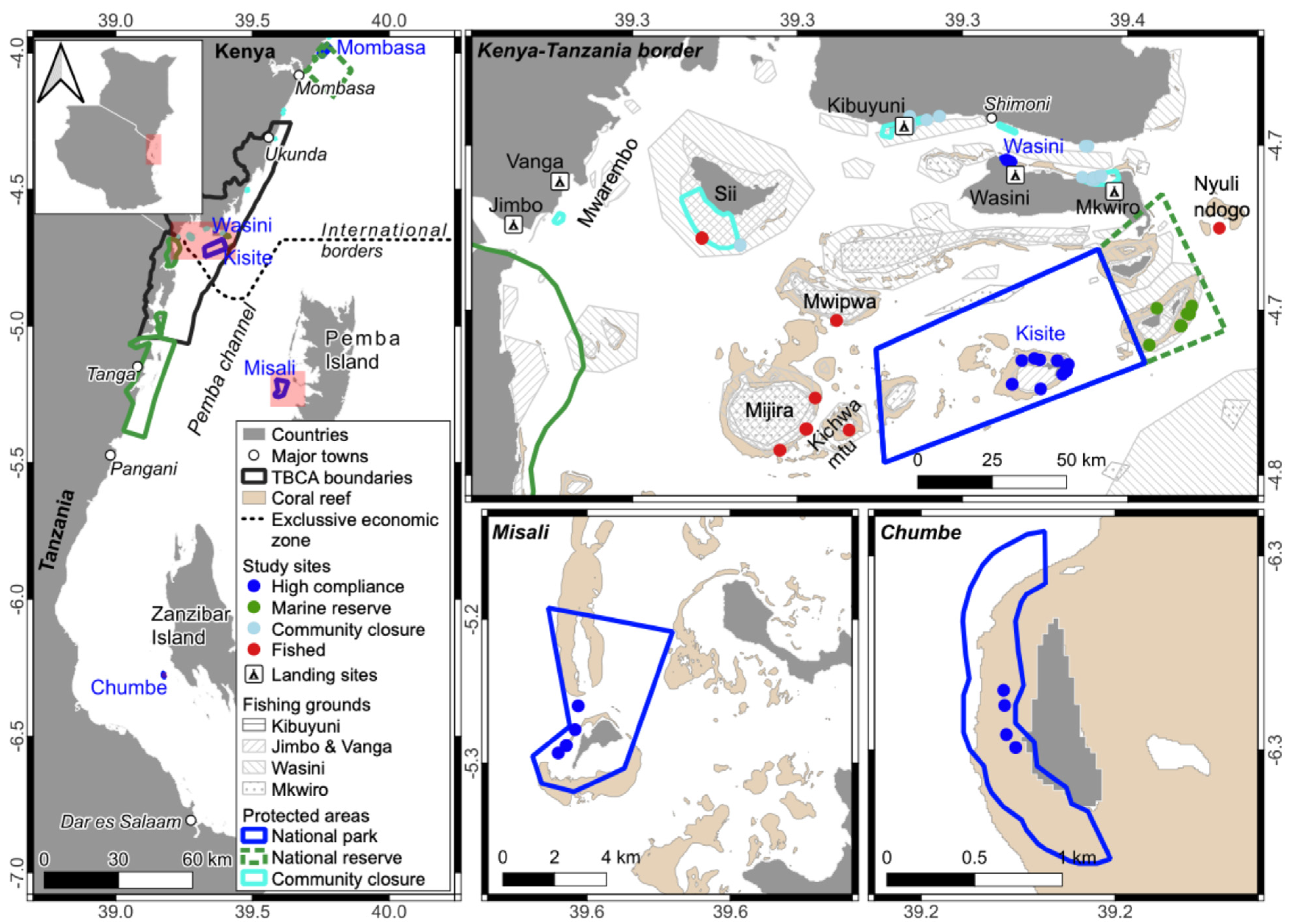
2.1. Study Sites

The southern Kenya–northern Tanzania location is a shallow marine environment with scattered coral reef islands located leeward of the emergent larger inhabited islands of Zanzibar and Pemba [17] (Figure 1). This marine lagoonal environment is approximately 30 km wide, 200 km long, and intersected by the deep Pemba Channel (~750 m deep). The lagoon runs from the south of the city of Dar es Salaam to the Shimoni–Vanga towns of Kenya in the north. It is characterized by low wave energy, cool water, and mildly variable temperatures, but with low acute thermal stress. The lagoon is inhabited by unique coral and fish assemblages that differ from the ocean-exposed windward environments [14]. Scattered small emergent and submerged reefs create high geomorphological and habitat diversity [14]. We studied fish communities in the 7 fisheries reserves in this lagoon as well as fish landings captured at 5 shoreline landing sites on the Kenyan side of the international border (Figure 1). The fished ecosystems are similar in being characterized by shallow nearshore sand, seagrass, and coral reefs, with some coastal fringing mangroves. The fished zones are predominantly characterized by a mixture of gear restrictions and occasional use of fish size limits, but no catch quotas. Enforcement is variable and dependent on local national and community governance commitments to national and protected area laws.

2.2. Field Methods

Estimates of the production of fishable and specific fish taxa in marine reserves and catch landing sites are described and compared below.

2.2.1. Fish Production Estimates from Marine Reserves

Fish stock censuses were undertaken to estimate biomass at the family/functional levels and numbers of individuals in preselected families at the species level between 1995 and 2023 (Supplementary Materials, Table S1a). The three government or privately managed marine reserves (Kisite, Chumbe, and Misali) were established in 1978, 1994, and 1998, and sampling was undertaken starting in 1995 and ending in 2023. The four community closures (Kibuyuni, Wasini, Mji wa Kale, and Sii) were established in 2008, 2009, 2015, and 2019, and sampling was undertaken between 2012 and 2021. More repeated sampling was undertaken in the reserves than in community closures. The differences in closure dates and ages provided a 45-year time series of biomass changes or recovery rates in closures.

Fishable biomass, defined as the biomass of fish > 10 cm in length in sampled transects, was evaluated. Following some precautions, this method is accurate for the larger observable fish captured by fishers [18]. Censuses were undertaken at irregular intervals between 1995 and 2023 on reef edges in a permanent national fisheries reserve established in 1978 (Kisite Marine National Park), with repeat sampling conducted in two fisheries reserves in Zanzibar (Chumbe Island closed in 1994) and on Pemba (Misali Island closed in 1998) and four smaller community managed reserves (Wasini, Sii, Kibuyuni, and Mji wa Kale). The 7 reserves were a mixture of national, private, and community reserves that varied in size from <1 to 34 km² (Supplementary Materials, Table S1a). These reserves represent reefs with various levels of connectivity and are separated by variable distances with a mean of 79.5 ± 33.8 km (±95% CI) (Supplementary Materials, Table S1b). Fished reefs in this region often have similar biomass with values of ~250 kg/ha that can be used to estimate the initial or pre-closure biomass [15]. The uniformity of initial biomass is expected to reduce the variation around the initial biomass conditions when reserves were closed to fishing. An exception was the Chumbe Island reserve, which was occupied and protected by the Tanzanian Navy prior to its establishment as a reserve in 1994, resulting in a higher early closure biomass (Figure 2a).

Underwater visual surveys used the same methods as belt transects of 500 m² over repeated sampling. Censuses were undertaken while snorkeling (<3 m) and SCUBA diving (3–15 m). Sites were a mixture of reef habitats including reef slopes, crests, and back reefs located on calcium carbonate bottoms colonized by hard and soft corals, algae, and sand, with seagrass being a smaller portion of the bottom cover. During surveys, individual fish within the belt were identified into 23 families and sized by standard lengths into 10 cm bins [15]. Individuals not in these 23 families were placed in an “Others” category. Several of the families had few captured species (i.e., Monocanthidae and Diodontidae) and were therefore not compared between the surveys and reserves. Taxa weights were estimated by using the midpoint of the size bins and published length–weight relationships taken from local landing sites to estimate the mean weight of each bin. Community biomass was therefore the sum of the bin weights in a censused transect and presented as kilograms per hectare for each and all taxonomic groups, but stocks and yields are presented as tons per square kilometer. Subsequent passes counted and identified fish to the species level for evaluations of species richness and for evaluating by-species differences in the proportionality of species in the censused reefs and fish landing sites.

2.2.2. Estimates of Proportional Taxonomic Composition and Linear Production

Proportionality is a measure of the balance between a fishery ecosystem taxa’s production and capture rates. To estimate this metric, fish counts in the oldest reserve were compared to catches. A total of 41 fish families were identified via both catch and reserve samples. Of the 41 families, 12 taxonomic groupings were captured at the landing sites and observed in the marine reserve census. This selection of 12 families was chosen to correct for potential biases. The 12 family/functional-based groupings included Acanthuridae, Chaetodontidae, Haemulidae, Holocentridae, Labridae, Lethrinidae, Lutjanidae, Mullidae, Pomacanthidae, Serranidae, and Siganidae. The Scarinae subfamily was kept separate from Labrinae due to ecological, functional, and catch-targeting differences when evaluating responses to fishing closure. Specifically, Scarinae species are herbivores while Labrinae species are carnivores The 12 common taxonomic groupings observed in catch and marine censuses were used in subsequent analyses including annual production rates, which were estimated as the change in biomass over time and based on the linear annual change (i.e., slope) in biomass. This was calculated for times series in the 7 reserves. In the oldest reserve (Kisite Marine National Park) and in the final year of field sampling, individual fish were counted and identified to the species level for these 12 shared families to evaluate differences between the oldest reserve and fish landings at the species level. Production estimates of fishable biomass used the common Schaefer or logistic model to test for potential exponential growth and to compare results with short-term (i.e., annual) stock catch production. Thus, these two estimates of production were compared for fit to empirical catch or capture production estimates from the landing sites (Figure 1), as described below.

2.2.3. Fisheries Catch Production Rates

Five fish landing sites were monitored by employed community members and fisheries department observers between February 2020 and June 2023 [19]. Data enumerators were selected based on their high scores on a previously described exam using a fisheries literacy test [19]. Additionally, the areas of the 5 landing sites’ fishing grounds were estimated via a collaborative community mapping process (Figure 1). It was established that there were 210 fishing days per year based on interviews and the landing site reports of fishing efforts. Therefore, these time and area estimates were used to calculate yields in tons on an annual or 210 fishing days per year basis.

Landing sites were visited 12.2 ± 0.3 (SEM) days per month by employed community members and 3.0 ± 0.2 days per month by fisheries officers. Observers recorded the numbers of fishers and boats and landed fish were weighed in as the following categories: octopus and five finfish catch group categories of goatfish, rabbitfish, scavengers, parrotfish, and mixed catch associated with benthic habitats. Each category was measured to the nearest 0.1 kg. The mixed catch was a diverse group of reef-associated fish that received a similarly low price. Landing data were entered via cell phones using KoboCollect mobile software (https://kf.kobotoolbox.org/accounts/login/, accessed on 4 July 2023, and data were downloaded into spreadsheets for subsequent analyses. Observers were instructed to measure catch from all fishers that landed fish. However, in some instances, a subsample (proportion of catch that fairly represents landed catch as per fish category and size) was measured.

2.2.4. Fish Length Estimates of Sustainability

Common length and spawning metrics were evaluated for their potential to estimate sustainability. Therefore, between August 2022 and August 2023, community data recorders sampled caught fish by measuring their total body lengths to the nearest centimeter. A total of 413 catch trips were recorded during sampling. Photos of all species were taken for identification and eventual validation of captured species. A total sample of 2284 individuals and 144 unique species of fish were measured, and these data were used to obtain length at first maturity (L_mat), length at optimum yield (L_opt), and spawning potential ratio (SPR) information for the well-sampled (n > 30) species. When catches were small, all fish captured were measured to the nearest millimeter and weighted to the nearest gram. The type of fishing gear and number of fishers and boats were recorded for each landing. When catches were large, a representative proportional sample was taken to measure lengths and weights.

To assist in identification, a list of species recorded in Kenya was compiled from Fishbase and unpublished government and non-government institutional sources (Supplementary Materials, Table S2), which assisted in the compilation of the list of species found in the studied reserves and catches (Supplementary Materials, Table S3). We classified species as either commercial or not based on their presence in the fish trade. The total fish species list for Kenya was based on catches and field observation and included 1034 species of which 204 were recorded in this study. Recorded species were pooled into the family for comparisons of differences between abundance in the reserve and catch samples.

2.3. Data Analyses

2.3.1. Production Estimates from Marine Reserves

Recovery of fish stocks in the 7 reserves were used to produce a plot of biomass as a function of the time since closure to fishing as an estimate of fish production in the absence of fishing. Stocks were estimated from replicate field transects that were pooled to sites and year to get a total of 35 site × time replications spanning 1 to 45 years of closure to fishing in reserves. Replicate transects undertaken in 14 adjacent fished sites were pooled and used to estimate the closure anchor year or the zero-recovery time point. Pooling transects or replicates standardizes sampling effort and improves data accuracy, minimizing variability.

Total surplus and annual production of the total biomass and 12 common taxonomic groups based on these replicates were plotted and data fit to logistic and linear models in the R package ‘nlsLM ()’. The reserve age–fishable biomass data were tested and compared for the Ricker, asymptote, and logistic models. The logistic model had the lowest Akaike information criterion (AIC) of 1495.6 compared to 1499.9 and 1514 for the asymptote and Ricker models, respectively. Therefore, the best-fit logistic was used to estimate the mean r (±95% CI) or the community biomass growth rate, K (±95% CI), the final mean equilibrium biomass, and the zero-age or the equations anchor point B₀ (±95% CI) (Supplementary Materials, Table S4a).

The logistic growth model is commonly used in fisheries data because it effectively captures population dynamics in fish stocks where resources are limited. Moreover, the logistic model is more resistant to overfitting and has higher predictive power than the other models. The surplus production model provides a foundation for sustainable fisheries management, offering simple tools to estimate the balance between production and capture and therefore estimate overfishing status. The model estimates sustainable harvest levels (maximum sustainable yields—MSYs) using recovery rate (r) and equilibrium biomass (K) from the logistic model, calculated as MSY = rK/4.

Coefficients and variance of the slope from linear regression models were used to estimate annual production for each taxonomic group (Supplementary Materials, Table S4b), thereby allowing by-taxa and sum or total production calculations. A linear model was used because reserve age (time) and total and taxonomic fishable biomass are independent of each other. Data were pooled such that samples were independent of each other and data fit assumptions of normality. The production estimates from linear and surplus models were compared to evaluate the influence of the exponential portion of the logistic model. All analyses were run in R version 4.2.1. Previous studies have focused on the recovery of various aspects of the coral reef community and habitat, but here the focus was on estimating stock production on a large scale that would match and be comparable with the above-described empirical fisheries catch data.

2.3.2. Proportional Taxonomic Composition and Production

To estimate taxa proportionality, fish counts in the oldest reserve were compared to counts in the catches for the 12 “family” groupings and the sampled species. Among the 12 groupings, a total of 192 species were identified of which 109 species were identified in the Kisite Marine National Park field transects (4500 m²) and 83 species in the catches (Supplementary Materials, Table S3). There were 69 species unique to the marine reserve, 43 species unique to the catches, and 40 species shared by both marine reserves and landings. The cumulative number of common species as a function of the number of individuals seen in the censuses or captured were compared for the reserve and fish landings. For comparisons, the species sold at landing sites (commercial) and taken for home consumption (noncommercial) were plotted separately to allow fairer comparisons of species richness in the reserves and catches. Commercial species were those species observed for sale in markets while noncommercial were species that were either not captured or, if captured, used for home consumption. Species abundance plots used function ‘iNEXT ()’ in iNEXT R package version 3.0.0.

One multivariate analysis of the fish community composition used all the recorded species in the marine reserves and catches. Relative abundances were calculated from the total sample of individuals per marine reserve and catch categories. Reserve and catch species composition were evaluated for associations or similarity by gear and landing site by Ward hierarchical clustering. Ward’s clustering was used because it minimizes the total within-cluster variance. Specifically, the method ensures clusters are as distinct and meaningful as possible where differences in species cluster patterns can be subtle.

To evaluate the associations distinguishing cluster groups, a Principal Component Analysis (PCA) using the Bray–Curtis’s distance matrix for species abundance with dominant gear types and sites as vectors is presented. This method was chosen because it handles compositional data and for its robustness to zeros. The PCA was conducted using the ‘fviz_pca_biplot ()’ package in R. Clustering evaluated the vectors of gear types, landing sites, and the reserve. A second analysis was conducted to evaluate the proportionality of relative fish abundance and production between the reserves and catches for the 12 groupings and the 40 shared species where proportionally equals ((Catch% − Reserve%)/Catch%) × 100. Catch and reserve percentages were obtained by standardizing the numbers of individuals of each species by the total numbers of individuals for all species in catches and reserves separately to allow comparisons. Additionally, we compared between-site differences in descriptive ecological metrics of dominance (D = Simpson index), diversity (H = Shannon index), and evenness (J) of censused and caught fish. Given the focus on between-site differences, samples collected over time were pooled to evaluate sites and gear changes. High diversity suggests high similarity while low diversity suggests high dissimilarity.

Taxonomic composition analyses compared catch traits by gear and landing sites. To determine if the differential abundance or proportionality reflected life history characteristics, we compiled their species traits from the FishLife package in R. Weighted life history traits were calculated as the trait frequency multiplied by the relative abundance of the species divided by the total number of species [20]. Comparisons were made regarding negative (more species in reserves) and positive (more species in catches) differential categories. Additionally, weighted values for catches based on each fishing gear were calculated.

2.3.3. Evaluation of Fisheries Catch Production Rates

Fisheries catch production rates were evaluated for standard fisheries metrics by landing sites and all sites combined. Metrics included days sampled per month, fishing effort calculated as numbers of fishers who fished on that day divided by size of fishing area (fisher/km²/day), catch-per-unit-effort (CPUE = kg/fisher/day) as total catch divided by numbers of fishers who fished, yield (kg/km²/day) as total catch divided by the size of fishing area, and income (Kenyan Shilling (KES)/fisher/day) summed as CPUE times the average price One United States dollar equaled ~120 KES in 2022. The same metrics were also presented for the common gear types of traps, spearguns, handlines, and gill nets. Additionally, subsamples enabled calculation of the mean length of all species, and the number of species caught per day for each gear. Finally, the same metrics were presented for the weighed catch groups of goatfish, mixed catch, octopus, parrotfish, pelagics, rabbitfish, and scavengers (i.e., Lutjanidae, Lethrinidae, Nemipheridae, and Haemulidae). These groupings were used by data collectors as these fit well with prices and were naturally grouped by fishers for sale.

Data presentations are organized from highest to lowest abundance in tables based on the sum of all sites. The empirical fish landing data were not normally distributed and therefore Kruskal–Wallis tests were used to test for statistical significance between landing sites and catch categories used in ‘dplyr’. Comparison between specific groups used the post hoc Dunn’s test with Bonferroni correction using ‘dunnTest ()’. The relationships between a landing site’s Yield/MSY and CPUE, trophic level, and the Shannon diversity index of the catches were plotted to evaluate the fish catch status difference among sites.

2.3.4. Length-Based Catch Indicators

Length and spawning metrics were evaluated to determine if they were useful in evaluating sustainability for modest sampling intensity. Three length metrics were considered: length at maturity (L_mat), mean length (L), and length at optimum yield (L_opt). L_mat represents the total length at which 50% of individuals are mature, L of a species in relation to L_mat is often used to inform recruitment overfishing status (e.g., [21,22]), and L_opt is derived from growth and mortality parameters or empirical equations [23] to indicate status relative to maximum sustainable yield (MSY). Thus, the L of a species in relation to L_opt is an indicator of growth overfishing. For sustainability, the L: L_mat and L: L_opt targets would therefore be 1 or greater. L_mat and L_opt values for all species were obtained from FishBase (Fishbase.org 2023). Relying on life history parameters from global databases is often necessary because these databases (i.e., FishBase) are often the only source for such information, particularly in data-poor contexts such as tropical coral reefs. However, this study acknowledges that this may not account for species-specific variability or data quality questions, like outdated information or an over-reliance on limited information. Therefore, both L: L_mat and L: L_opt for all species in the catches where sample sizes were adequate (n > 30) were calculated as well as their 95% confidence intervals.

The final metric evaluated was the spawning potential ratio (SPR). The SPR is the proportion of the unfished reproductive potential left at the given fishing pressure [24]. The SPR was calculated for the most abundant species in the catch data (n > 30) using a length-based method (LBSPR) that requires the natural mortality to growth rate (M/k) ratio, asymptotic length, length at 50% maturity, and length at 95% maturity. SPR uses a length-per-recruit-structured model that splits the stock into diverse sub-cohorts, or growth-type groups, to account for length-dependent fish mortality rates [25]. The LBSPR model used life history parameters from FishBase [26] or the FishLife package in R [27,28], which uses a Bayesian modeling approach to predict parameters. The LBSPR method is sensitive to non-equilibrium dynamics, M/k estimation, and the shape of the capture selectivity curve [25]. The purpose here was to evaluate if this method, as commonly used, would be useful for estimating sustainability. Determining if these assumptions were correct would require more data and long-term analyses. To estimate sustainability, we used the suggestion that SPR values of 40% or greater are considered healthy and risk-averse [29]. SPR values between 25–40% indicate the stock may be overfished, and values below 25% indicate the stock is likely overfished.

3. Results

3.1. Production of Fish

3.1.1. Recovery Rate and Production Estimates from Marine Reserves

Biomass recovery of total reef fish stock determined from the space-for-time substitution found K, B₀, and r were all strongly statistically significant (p < 0.008) (Figure 2a; Supplementary Materials, Table S4a). The best-fit logistic model had a final equilibrium biomass of 1532 ± 605 (±2 SEM or 95%CI), an initial biomass (B₀) of 298.7 ± 148, and a mean recovery rate, or r, of 0.09 ± 0.06. Consequently, the estimated mean MSY was 3.83 tons/km²/year, but the high 95% CI indicates it could range greatly. In the unlikely case that the highest and lowest biomass and production coincided, the production would range from 1.2 to 15.6 tons/km²/year. In the more likely case that high biomass corresponds to low production and vice versa, the production range would range from 2.7 to 3.9 tons/km²/year. The annual change linear model estimate of total biomass production was 2.8 ± 0.6 tons/km²/y (p < 0.0001; R² = 0.70).

Recovery rate fits for the 12 taxonomic groupings indicated considerable variability and largely non-significant fits to the logistic model (Figure 2b; Supplementary Materials, Table S4a). Only K values were consistently statistically significant with no significance found for B₀ and r variables among all groupings. Poor fit to the logistic model contrasted with the linear production model that found significant reserve age slopes or annual production rates for Acanthuridae, Balistidae, Haemulidae, Others, Chaetodontidae, Pomacanthidae, Holocentridae, Labrinae, Lutjanidae, Mullidae, Scarinae, Serranidae, and total biomass (Supplementary Materials, Table S4b). The fit to the total biomass and Balistidae had the strongest relationships with time, R² of 0.70 and 0.50, respectively.

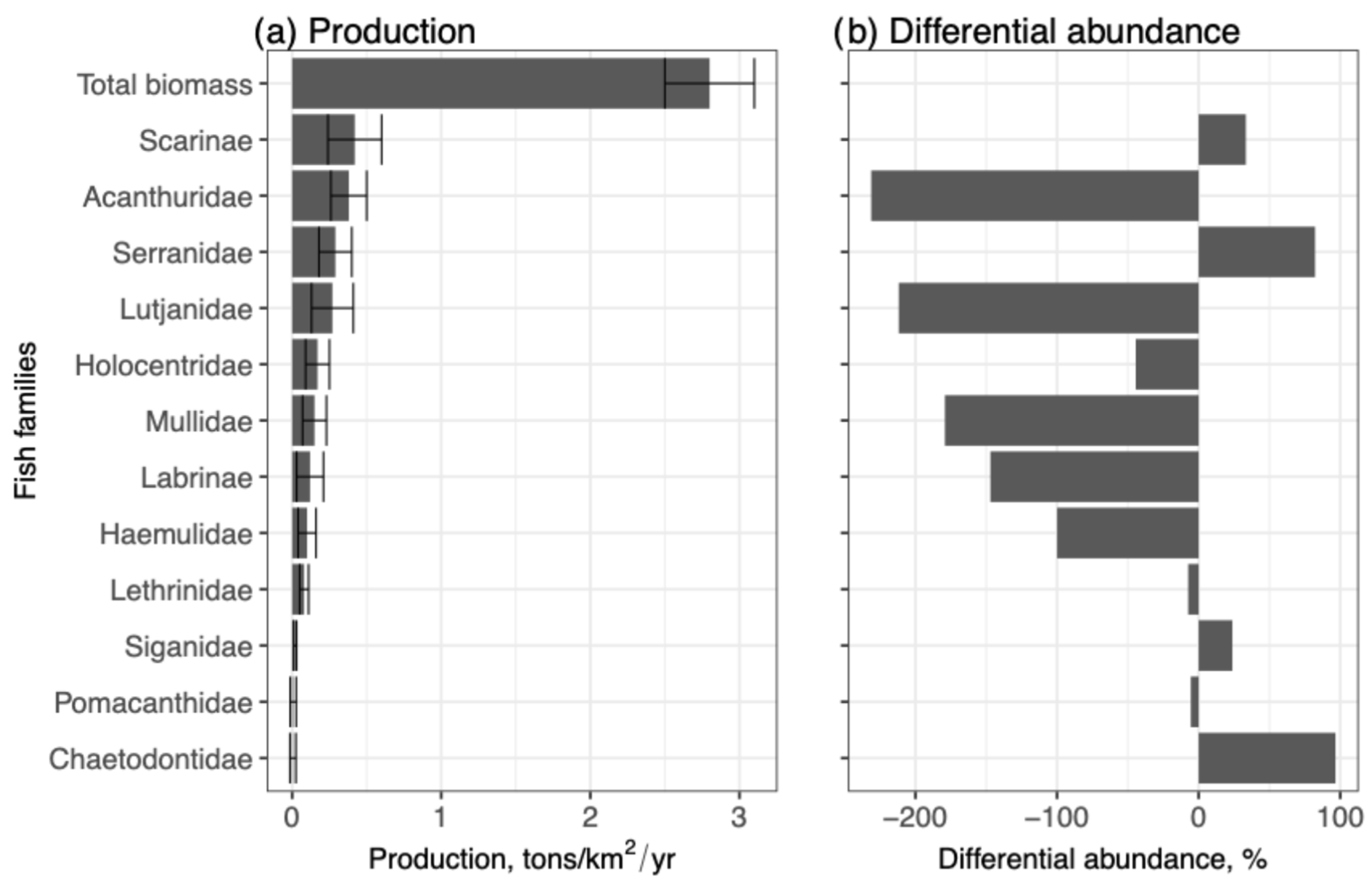
3.1.2. Family/Functional-Level Annual Production

Estimates of total annual linear production summing the 12 fish family/functional groupings in reserves indicated a total fishable production of 2.8 ± 0.7 tons/km²/year (Figure 3a). The Scarinae subfamily was the greatest contributor to annual production, followed by Acanthuridae, Serranidae, Lutjanidae, Holocentridae, Mullidae, Labrinae, Haemulidae, Lethrinidae, and Siganidae. Pomacanthidae and Chaetodontidae did not show any significant measurable annual production.

Comparing differences in the relative biomass of the fish groupings between the oldest reserve and the catch samples indicated a poor match between ranked estimates of production and the differential biomass (Figure 3b). Acanthuridae, Lutjanidae, Mullidae, Labrinae, Haemulidae, and Holocentridae were families with large negative differentials, which indicates significant lost potential production by these families. In contrast, Chaetodontidae, Serranidae, Scarinae, and Siganidae had smaller positive differentials that suggest little potential compensation in their production among these groups.

3.1.3. Estimated Fisheries Catch

Catch sampling among the 210 fishing days per year was undertaken for 11.7 ± 0.6 (±2 SEM) days per month. The 1.77 ± 0.16 fishers/km² caught 1.80 ± 0.16 kg/day producing a per fisher income of 772 ± 64 KES/fisher/day or USD 6.4 per day (

Table 1. Landed fish catch statistics. Means and standard errors of the mean (±SE) statistics by site and all sites for catches recorded over a 30-month period for (a) sampling, sampled days per month, sample size, fishing effort (fishers/km²/day), catch-per-unit-effort (CPUE, kg/fisher/day), income (KES/fisher/day), yield (kg/km²/day), and yield (tons/km²/y). (b) The site and all sites CPUE, yield, and income for dominant fish groups. Kruskal–Wallis and post hoc Dunn’s tests of significance are presented. Fisheries catch data are based on 1635 catch trips at 5 fish landing sites collected between February 2021 and December 2023. Values that share the same superscripted letters are not statistically different from each other.

	Category	Mkwiro	Wasini	Kibuyuni	Vanga	Jimbo	ChiSq; Prob > ChiSq	All Sites
(a) Sampling	Days sampled/month	13.6 ± 0.9 a	11.5 ± 0.7 b	11.9 ± 0.7 b	11.7 ± 0.6 b	10.0 ± 0.6 c	17.1; 0.002	11.7 ± 0.3
	Sample size (n)	366	320	345	318	286		1635
	Effort (Fishers/km2/day)	2.06 ± 0.16 a	1.85 ± 0.1 a	2.56 ± 0.28 b	1.29 ± 0.06 c	1.15 ± 0.08 c	63.6; <0.0001	1.77 ± 0.08
	CPUE (kg/fisher/day)	5.58 ± 0.28 a	3.46 ± 0.24 b	4.11 ± 0.2 b	2.4 ± 0.08 c	3.51 ± 0.21 b	75.0; <0.0001	3.79 ± 0.13
	Income (KES/fisher/day)	1214.76 ± 56.06 a	920.43 ± 66.62 b	841.12 ± 40.59 b	374.14 ± 17.58 c	548.89 ± 37.03 c	94.7; <0.0001	772.27 ± 32.03
	Yield (kg/km2/day)	11.95 ± 1.35 a	6.96 ± 0.69 b	9.99 ± 0.91 b	2.9 ± 0.17 c	3.6 ± 0.19 c	90.2; <0.0001	6.99 ± 0.45
	Yield (tons/km2/y)	2.53 ± 0.29 a	1.48 ± 0.15 b	2.12 ± 0.19 b	0.62 ± 0.04	0.76 ± 0.04 c	90.2; <0.0001	1.48 ± 0.10
(b) Fish groups
CPUE	Goatfish	0.13 ± 0.01 a	0.06 ± 0.01 b	0.11 ± 0.02 b	0.04 ± 0.01 c	0.01 ± 0.004 c	70.4; <0.0001	0.07 ± 0.01 a
	Mixed catch	0.43 ± 0.04 a	0.25 ± 0.02 c	0.19 ± 0.01 c	0.60 ± 0.07 a	0.76 ± 0.09 b	68.7; <0.0001	0.44 ± 0.03 b
	Octopus	0.21 ± 0.03 a	0.22 ± 0.03 a	0.39 ± 0.03 a	0.30 ± 0.03 a	0.97 ± 0.09 b	59.4; <0.0001	0.41 ± 0.03 b
	Parrotfish	0.28 ± 0.02 a	0.20 ± 0.03 b	0.17 ± 0.02 b	0.15 ± 0.03 b	0.10 ± 0.02 b	26.8; <0.0001	0.18 ± 0.01 c
	Pelagics	0.20 ± 0.03 a	0.26 ± 0.04 a	0.17 ± 0.03 a	0.60 ± 0.08 b	0.46 ± 0.08 b	42.3; <0.0001	0.34 ± 0.03 d
	Rabbitfish	0.58 ± 0.07 a	0.40 ± 0.04 b	0.33 ± 0.02 c	0.23 ± 0.04 c	0.33 ± 0.08 c	32.7; <0.0001	0.37 ± 0.03 b
	Scavengers	0.50 ± 0.03 a	0.33 ± 0.03 a	0.22 ± 0.02 b	0.97 ± 0.11 c	0.61 ± 0.09 a	51.3; <0.0001	0.52 ± 0.04 e
Yield	Goatfish	0.11 ± 0.02 a	0.03 ± 0.01 b	0.06 ± 0.01 b	0.01 ± 0.002 c	0.003 ± 0.002 c	88.5; <0.0001	0.04 ± 0.01 a
	Mixed catch	0.42 ± 0.07 a	0.16 ± 0.02 b	0.17 ± 0.03 b	0.32 ± 0.04 c	0.25 ± 0.03 c	22.0; 0.0002	0.27 ± 0.02 b
	Octopus	0.07 ± 0.01 a	0.10 ± 0.02 a	0.38 ± 0.07 b	0.17 ± 0.02 a	0.47 ± 0.05 b	62.9; <0.0001	0.24 ± 0.02 b
	Parrotfish	0.25 ± 0.04 a	0.11 ± 0.02 b	0.15 ± 0.02 b	0.05 ± 0.01 c	0.04 ± 0.01 c	55.5; <0.0001	0.12 ± 0.01 c
	Pelagics	0.09 ± 0.02 a	0.22 ± 0.05 a	0.13 ± 0.04 a	0.34 ± 0.02 b	0.23 ± 0.04 a	42.2; <0.0001	0.20 ± 0.02 d
	Rabbitfish	0.60 ± 0.09 a	0.45 ± 0.07 a	0.54 ± 0.06 a	0.05 ± 0.01 b	0.08 ± 0.02 b	85.3; <0.0001	0.34 ± 0.03 e
	Scavengers	0.52 ± 0.04 a	0.32 ± 0.03 a	0.31 ± 0.06 a	0.12 ± 0.02 b	0.17 ± 0.02 b	50.2; <0.0001	0.29 ± 0.02 b
Income	Goatfish	29.66 ± 3.00 a	17.57 ± 2.80 a	22.75 ± 2.90 a	6.98 ± 2.34 b	1.95 ± 0.81 b	74.1; <0.0001	15.79 ± 1.41 a
	Mixed catch	71.87 ± 7.16 a	51.47 ± 4.83 a	26.65 ± 2.05 b	68.33 ± 7.22 a	81.17 ± 8.89 c	46.9; <0.0001	59.53 ± 3.28 b
	Octopus	49.35 ± 6.65 a	61.73 ± 8.09 b	97.15 ± 7.76 c	72.59 ± 7.82 b	184.25 ± 20.38 d	49.3; <0.0001	92.30 ± 6.37 c
	Parrotfish	49.89 ± 4.77 a	47.00 ± 6.02 a	25.25 ± 2.49 b	23.81 ± 4.90 c	11.45 ± 2.74 c	46.9; <0.0001	31.35 ± 2.30 a
	Pelagics	47.64 ± 7.07 a	69.25 ± 10.44 a	39.00 ± 6.28 a	85.86 ± 12.96 b	77.94 ± 14.69 a	14.4; 0.006	63.93 ± 4.99 b
	Rabbitfish	149.99 ± 19.75 a	114.39 ± 10.77 a	70.18 ± 4.69 b	51.49 ± 10.02 b	64.34 ± 16.48 b	45.1; <0.0001	88.61 ± 6.57 c
	Scavengers	118.19 ± 8.67 a	92.50 ± 8.79 a	44.39 ± 4.87 b	168.2 ± 17.56 c	87.20 ± 12.90 a	48.2; <0.0001	100.84 ± 6.04 c

). This effort produced 7.0 ± 0.9 kg/km²/day (1.48 ± 0.2 tons/km²/y), but high variability was recorded between landing sites and catch metrics. In terms of CPUE, Mkwiro had the highest daily catch rate, Vanga the lowest, and Wasini, Kibuyuni, and Jimbo had intermediate rates. Per area, yields showed similar patterns with Mkwiro having nearly twice the average and Vanga and Jimbo nearly half the average yields. Differences between landing sites were also recorded for the catch groups. For CPUE, the importance of the taxa decreased from scavengers to mixed catch, octopus, rabbitfish, pelagics, parrotfish, and goatfish. Rabbitfish, scavengers, and octopus contributed most to yields and income, but these taxa were caught less at the Vanga and Jimbo landing sites. Pelagic fish were the most important portion of the catch at Vanga and octopus in Jimbo.

3.1.4. Numbers of Fish Species

Among the 12 fish groupings, species accumulation curves indicate similar rates of rise in the number of species in the old Kisite Marine National Park versus in fish catches pooled for all landing sites up to 2000 counted individuals (Figure 4). Above 2000 individuals, the marine reserve accumulated more species, up to 109 species at 4978 individuals, than the catch samples. Accumulation of species in landing sites is largely due to commercial species while there is a more balanced mix of commercial and noncommercial species in the marine reserve. At the landing site level, the number of caught species was markedly lower than the sum of all landing sites, rarely exceeding 50 species per 4000 individuals.

3.2. Balanced Harvest Analyses

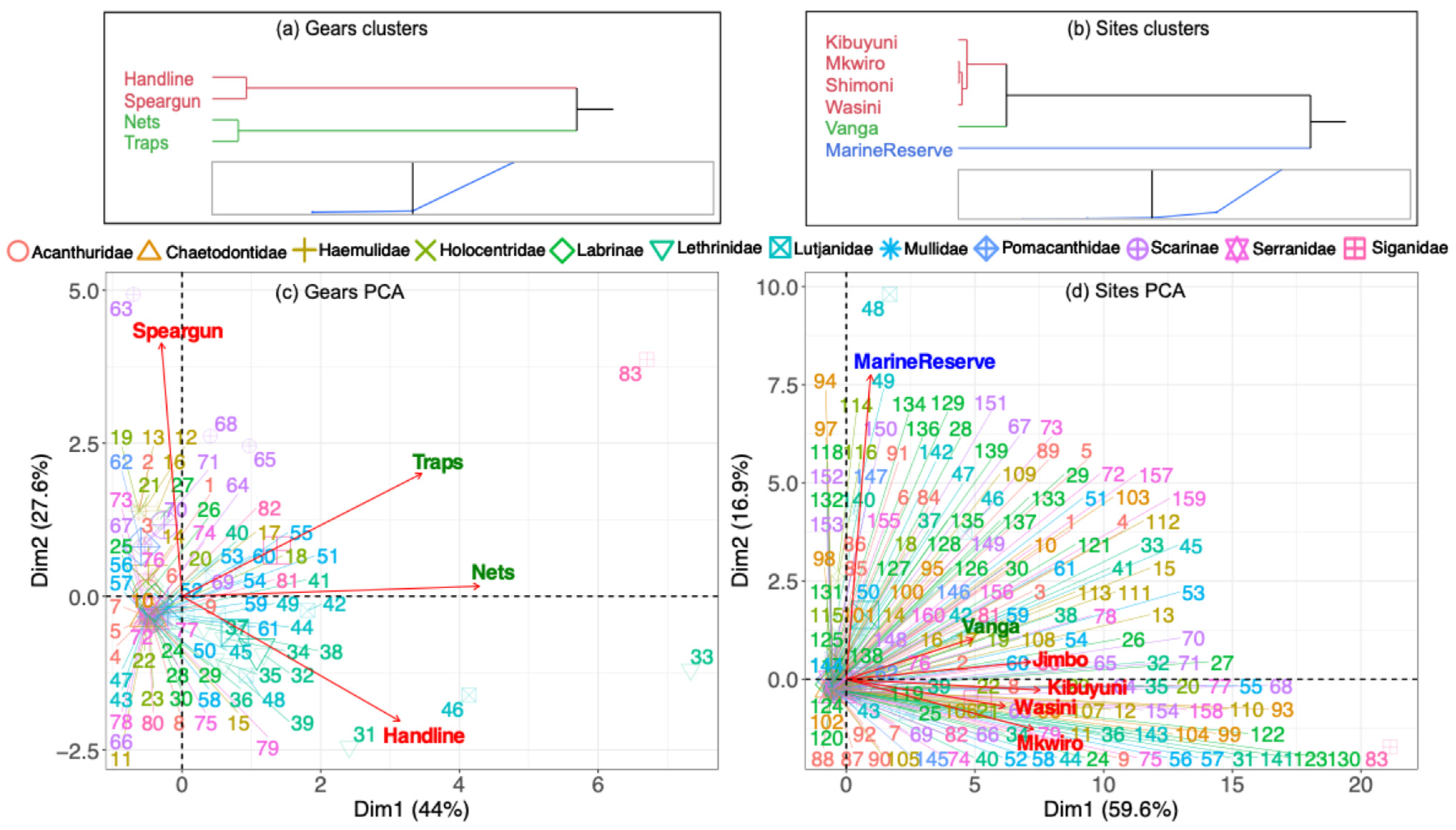
3.2.1. Balanced Gear Analyses

Multivariate analyses suggest some significant groupings or distinctions in species composition by gear and landing sites (Figure 5). Handlines and spears formed a unique cluster as did traps and nets. Differences among gear types (as shown by the vectors) were largely driven by a few species that were more common in the catch of each gear type (Figure 5a). For example, handlines captured relatively more Lutjanus fulviflamma and L. kasmira snappers. Traps and nets captured more Siganus sutor rabbitfish and spearguns more Calotomus carolina and Scarus ghobban parrotfishes. The catch composition in the marine reserve and Vanga cluster was different from the Jimbo, Kibuyuni, Wasini, and Mkwiro landing site clusters (Figure 5b). Lutjanus kasmira and L. lutjanus were one of the most common species in the marine reserve while several parrotfish were most common in the fisheries catch. Vanga’s catch was more like the reserve than Jimbo, Kibuyuni, Wasini, and Mkwiro, which may be due to differences in the total number of species caught. Consequently, there were two groups of distinct gear niches, and Vanga was a unique site in capturing many species but with low dominance and yields. Nevertheless, many species were caught by most gear types.

The mean lengths of fish were generally small at 22.0 ± 0.2 cm with modest differences among gear types (

Table 2. (a) Numbers of unique species caught by gear, site, and totals. Means and standard errors of the mean (±SE) and sample sizes by site, gear, and totals for (b) fish length measured nearest to millimeter, (c) catch-per-unit-effort (CPUE, kg/fisher/day), (d) yield (kg/km²/day), and (e) income (KES/fisher/day). Kruskal–Wallis and post hoc Dunn’s tests of significance are presented. Table 2a,b were generated using 2281 individuals of species collected between August 2022 and December 2023. Table 2c–e were summarized from 1635 catch trips collated between February 2021 and December 2023. Both datasets in Table 2a,b and Table 2c–e were collected at 5 fish landing sites. NS = not statistically significant. Values that share the same superscripted letters are not statistically different from each other.

	Category	Mkwiro (n)	Wasini (n)	Kibuyuni (n)	Vanga (n)	Jimbo (n)	ChiSq; Prob > ChiSq	All Sites (n)
(a) Number of species	Traps	30	16	28	32	22		66
	Spearguns	0	5	0	7	20		27
	Handlines	8	0	15	9	9		29
	Nets	0	2	6	88	5		93
	All gear types	34	21	30	104	43
(b) Fish length	Traps	28.0 ± 0.5 (151) a	25.0 ± 0.8 (63) b	27.0 ± 0.4 (178) b	22.0 ± 0.4 (226) c	28.0 ± 0.8 (100) b	120.6; <0.0001	26.0 ± 0.3 (718) b
	Spearguns		24.0 ± 1.1 (15) a		23.0 ± 1.0 (11) a	26.0 ± 1.5 (33) a	NS	25.0 ± 0.9 (59) b
	Handlines	19.0 ± 0.8 (15) a	34.0 ± 1.0 (6) b	20.0 ± 1.0 (58) a	20.0 ± 0.4 (37) a	22.0 ± 1.1 (23) b	18.8; 0.0009	21.0 ± 0.5 (139) a
	Nets		19.0 ± 0.2 (20) a	26.0 ± 0.7 (33) b	19.0 ± 0.2 (840) a	19.0 ± 0.9 (10) a	27.6; <0.0001	19.0 ± 0.2 (903) a
	All gear types	28.0 ± 0.5 (166) a	24.0 ± 0.6 (104) b	25.0 ± 0.4 (269) a	20.0 ± 0.2 (1114) c	26.0 ± 0.6 166) a	292.5; <0.0001	22.0 ± 0.2 (1819)
(c) CPUE	Traps	5.45 ± 0.33 a	3.41 ± 0.27 b	4.47 ± 0.23 a	6.94 ± 0.51 c	4.85 ± 0.37 a	46.1; <0.0001	5.05 ± 0.19 a
	Spearguns	3.93 ± 0.37 a	3.28 ± 0.23 a	3.34 ± 0.18 a	3.41 ± 0.23 a	3.73 ± 0.21 a	NS	3.51 ± 0.11 b
	Handlines	5.1 ± 0.31 a	2.82 ± 0.27 a	3.48 ± 0.24 a	3.38 ± 0.34 a	2.84 ± 0.17 b	35.9; <0.0001	3.52 ± 0.14 b
	Nets	3.25 ± 0.46 a	4.08 ± 0.3 b	4.16 ± 0.4 c	3.18 ± 0.24 b	2.88 ± 0.26 c	16.9; 0.002	3.48 ± 0.14 c
	All gear types	4.64 ± 0.2 a	3.61 ± 0.17 b	3.82 ± 0.15 b	3.8 ± 0.19 b	3.37 ± 0.15 b	33.7; <0.0001	3.77 ± 0.08
(d) Yield	Traps	6.93 ± 1.07 a	3.35 ± 0.43 b	4.92 ± 0.49 c	0.67 ± 0.05 d	1.09 ± 0.14 d	87.6; <0.0001	3.39 ± 0.32 a
	Spearguns	1.05 ± 0.1 a	0.99 ± 0.09 a	2.74 ± 0.33 b	1.37 ± 0.13 a	1.5 ± 0.15 a	26.5; <0.0001	1.59 ± 0.1 c
	Handlines	3.71 ± 0.44 a	1.17 ± 0.15 b	2.2 ± 0.39 c	0.29 ± 0.04 d	0.62 ± 0.06 d	69.6; <0.0001	1.68 ± 0.17 b
	Nets	1.08 ± 0.13 a	2.66 ± 0.23 b	3.25 ± 0.48 b	1.08 ± 0.06 a	1.55 ± 0.14 a	51.7; <0.0001	1.87 ± 0.1 c
	All gear types	3.52 ± 0.42 a	2.16 ± 0.15 b	3.21 ± 0.22 a	0.99 ± 0.04 c	1.3 ± 0.08 c	130.6; <0.0001	2.04 ± 0.08
(e) Income	Traps	1215.04 ± 68.75 a	916.15 ± 77.57 b	873.11 ± 46.77 b	1030.59 ± 68.24 b	715.65 ± 64.23 c	29.1; <0.0001	955.8 ± 32.25 a
	Spearguns	924.93 ± 88.34 a	892.86 ± 66.6 a	718.03 ± 36.75 a	746.13 ± 45.79 a	692.56 ± 47.84 a	NS	790.39 ± 26.45 c
	Handlines	1093.29 ± 63.82 a	736.76 ± 72.45 b	674.35 ± 47.23 b	605.34 ± 90.25 b	366.21 ± 20.29 c	58.9; <0.0001	697.55 ± 33.7 b
	Nets	686.99 ± 109.17 a	1056.54 ± 80.74 b	822.24 ± 85.34 b	491.23 ± 44.39 a	436.81 ± 49.46 a	70.8; <0.0001	678.73 ± 34.34 d
	All gear types	1033.58 ± 43.59 a	950.76 ± 44.63 a	769.32 ± 29.64 b	622.49 ± 33.58 c	529.5 ± 28.53 c	126.5; <0.0001	757.29 ± 17.91

). Nets captured the smallest (19.0 ± 0.2 cm), followed by handlines (21.0 ± 0.5) and spearguns (25.0 ± 0.9), and traps captured the largest fish (26.0 ± 0.3). Traps also had the highest CPUE, yields, and incomes. Spearguns and handlines were intermediate and did not differ in CPUE while nets had the lowest CPUE and income values. Gear types had high diversity and evenness of catch but generally declined along a spearguns, traps, nets, and handlines sequence (

Table 3. Simpson, Shannon, and evenness diversity indices for (a) dominant gear types and (b) study sites. Gear summaries were compiled from all 83 fish species identified in 12 common families in catch landing data. Site summaries were compiled from all 160 fish species identified in 12 common families during both catch and field sampling. Data were collected from 5 landing sites between August 2022 and December 2023.

	Simpson Index	Shannon Index	Evenness
(a) Gear
Speargun	0.93	2.86	1.0
Traps	0.82	2.67	0.93
Nets	0.88	2.61	0.91
Handline	0.90	2.55	0.89
(b) Site
Marine reserve	0.92	3.27	1.0
Jimbo	0.94	3.15	0.97
Vanga	0.88	2.77	0.85
Mkwiro	0.81	2.47	0.76
Wasini	0.87	2.44	0.75
Kibuyuni	0.79	2.30	0.70

a).

3.2.2. Balanced Taxonomic Composition Analyses

Evaluating the number of individuals in the 12 family/functional groupings and 40 species shared by the catch and reserve samples indicated large differences in the relative abundance of families and species (

Table 4. Summaries of common (a) families and (b) species abundance (mean ± standard deviation, SD) and sample size (n) of fish landing sampling at 5 sites (catch landing) and field sampling using discrete group sampling (DGS) transects at Kisite Marine National Park (MNP). Species are based on the 40 species in common in the census and fish landing data. Percentages of total and coefficients of variations (COV, %) for catch landing and field sampling are presented as well as percentage differential abundance between catch and field sampling of the unfished Kisite Marine National Park [(catch% − reserve%)/catch% × 100]. Simpson dominance, Shannon diversity, and evenness indices are presented for family and species. The table data are ordered from most negative to most positive differential abundances. Fish landing data were summarized from 753 individuals sampled between August 2022 and December 2023 while 2881 individuals sampled in May 2023 were used for the field survey data.

	Fish Landing Sampling			Field Sampling (DGS)
	Numbers/Fishing Group/Day ± SD (n)	Percentage of Total	COV, %	Numbers/500 m2 ± SD (n)	Percentage of Total	COV, %	Differential Abundance, %
(a) Family
Acanthuridae	0.01 ± 0.11 (12)	1.6	1928.8	3.38 ± 7.62 (152)	5.3	225.7	−231.3
Lutjanidae	0.03 ± 0.40 (13)	1.7	1277.2	17.11 ± 19.59 (154)	5.3	114.5	−211.8
Mullidae	0.09 ± 0.65 (192)	25.5	699.9	45.56 ± 133.93 (2050)	71.2	294	−179.2
Labrinae	0.01 ± 0.13 (13)	1.7	1622	3.33 ± 12.41 (120)	4.2	372.4	−147.1
Haemulidae	0.005 ± 0.10 (2)	0.3	2032.2	2.0 ± 1.8 (18)	0.6	90.1	−100
Holocentridae	0.01 ± 0.13 (7)	0.9	1588	2.11 ± 3.63 (38)	1.3	171.9	−44.4
Lethrinidae	0.01 ± 0.10 (20)	2.7	1419.3	1.33 ± 2.37 (84)	2.9	177.7	−7.4
Pomacanthidae	0.02 ± 0.25 (27)	3.6	1169.5	4.07 ± 7.98 (110)	3.8	195.8	−5.6
Siganidae	0.01 ± 0.01 (16)	2.1	100	1.0 ± 1.57 (45)	1.6	156.7	23.8
Scarinae	0.005 ± 0.07 (2)	0.3	1435.3	0.56 ± 0.73 (5)	0.2	130.8	33.3
Serranidae	0.04 ± 0.37 (89)	11.8	865.4	1.33 ± 1.82 (60)	2.1	136.6	82.2
Chaetodontidae	0.87 ± 2.04 (360)	47.8	234.3	5.0 ± 11.63 (45)	1.6	232.6	96.7
Simpson index	0.69			0.48
Shannon index	1.53			1.16
Evenness	1			0.76
(b) Species
Gomphosus caeruleus	0.049 ± 0.002 (1)	0.1	4.9	5.6 ± 3.5 (50)	1.74	63.7	−1640
Lutjanus kasmira	0.46 ± 0.05 (20)	2.7	10.5	124.2 ± 250.7 (1118)	38.81	201.8	−1337.4
Lutjanus gibbus	0.049 ± 0.002 (1)	0.1	4.9	4.3 ± 8.9 (39)	1.35	205.1	−1250
Naso annulatus	0.098 ± 0.005 (2)	0.3	4.9	12.4 ± 13.8 (112)	3.89	110.6	−1196.7
Myripristis berndti	0.139 ± 0.01 (4)	0.5	7	11.7 ± 23.8 (105)	3.64	203.8	−628
Mulloidichthys vanicolensis	0.148 ± 0.01 (3)	0.4	4.9	6.8 ± 13.3 (61)	2.12	195.7	−430
Ctenochaetus striatus	0.049 ± 0.002 (1)	0.1	4.9	1.4 ± 1.7 (13)	0.45	120.5	−350
Aethaloperca rogaa	0.049 ± 0.002 (1)	0.1	4.9	1.2 ± 1.4 (11)	0.38	114.1	−280
Lutjanus lutjanus	0.462 ± 0.08 (35)	4.6	18.3	53.3 ± 138.9 (480)	16.66	260.5	−262.2
Cephalopholis argus	0.098 ± 0.005 (2)	0.3	4.9	3.2 ± 1.8 (29)	1.01	55.5	−236.7
Lethrinus obsoletus	0.402 ± 0.03 (13)	1.7	7.8	17.1 ± 19.6 (154)	5.35	114.5	−214.7
Scarus frenatus	0.07 ± 0.005 (2)	0.3	7	2.4 ± 2.0 (22)	0.76	82.1	−153.3
Plectorhinchus gaterinus	0.12 ± 0.01 (4)	0.5	8.1	4.0 ± 4.4 (36)	1.25	111.1	−150
Chaetodon auriga	0.098 ± 0 (2)	0.3	4.9	2.0 ± 1.8 (18)	0.62	90.1	−106.7
Thalassoma lunare	0.049 ± 0 (1)	0.1	4.9	0.6 ± 0.7 (5)	0.17	130.8	−70
Halichoeres hortulanus	0.085 ± 0.01 (3)	0.4	8.5	2.1 ± 1.7 (19)	0.66	80.1	−65
Acanthurus leucosternon	0.148 ± 0.01 (3)	0.4	4.9	1.9 ± 2.9 (17)	0.59	155.4	−47.5
Parupeneus barberinus	0.322 ± 0.03 (13)	1.7	9.8	5.3 ± 1.7 (48)	1.67	32.5	1.8
Lutjanus fulviflamma	0.824 ± 0.28 (116)	15.4	34.1	45.8 ± 71.9 (412)	14.3	157.1	7.1
Acanthurus nigricauda	0.07 ± 0.005 (2)	0.3	7	0.8 ± 1.0 (7)	0.24	124.9	20
Sargocentron caudimaculatum	0.098 ± 0.005 (2)	0.3	4.9	0.8 ± 1.6 (7)	0.24	201	20
Scarus psittacus	0.13 ± 0.01 (5)	0.7	9.3	1.7 ± 1.8 (15)	0.52	108.2	25.7
Pomacanthus imperator	0.07 ± 0.005 (2)	0.3	7	0.6 ± 0.7 (5)	0.17	130.8	43.3
Myripristis murdjan	0.148 ± 0.01 (3)	0.4	4.9	0.4 ± 1.0 (4)	0.14	228.1	65
Calotomus carolinus	0.36 ± 0.04 (16)	2.1	10.8	2.1 ± 2.2 (19)	0.66	104.4	68.6
Anampses caeruleopunctatus	0.049 ± 0.002 (1)	0.1	4.9	0.1 ± 0.3 (1)	0.03	300	70
Bodianus bilunulatus	0.049 ± 0.002 (1)	0.1	4.9	0.1 ± 0.3 (1)	0.03	300	70
Epinephelus spilotoceps	0.049 ± 0.002 (1)	0.1	4.9	0.1 ± 0.3 (1)	0.03	300	70
Cheilinus trilobatus	0.098 ± 0.01 (4)	0.5	9.9	0.4 ± 0.5 (4)	0.14	118.6	72
Sargocentron diadema	0.12 ± 0.01 (4)	0.5	8.1	0.4 ± 1.0 (4)	0.14	228.1	72
Acanthurus dussumieri	0.155 ± 0.01 (4)	0.5	6.2	0.3 ± 0.7 (3)	0.1	212.1	80
Plectorhinchus flavomaculatus	0.148 ± 0.01 (3)	0.4	4.9	0.2 ± 0.4 (2)	0.07	198.4	82.5
Cheilio inermis	0.202 ± 0.02 (9)	1.2	10.8	0.4 ± 0.7 (4)	0.14	163.5	88.3
Epinephelus merra	0.07 ± 0.005 (2)	0.3	7	0.1 ± 0.3 (1)	0.03	300	90
Cephalopholis boenak	0.26 ± 0.02 (10)	1.3	9.3	0.3 ± 0.5 (3)	0.1	150	92.3
Scarus rubroviolaceus	0.109 ± 0.01 (5)	0.7	11.1	0.1 ± 0.3 (1)	0.03	300	95.7
Siganus sutor	2.042 ± 0.87 (360)	47.8	42.7	5.0 ± 11.6 (45)	1.56	232.6	96.7
Parupeneus cyclostomus	0.264 ± 0.03 (11)	1.5	10.1	0.1 ± 0.3 (1)	0.03	300	98
Scarus ghobban	0.721 ± 0.15 (61)	8.1	20.5	0.3 ± 1.0 (3)	0.1	300	98.8
Lutjanus argentimaculatus	0.984 ± 0.05 (20)	2.7	4.9	0.1 ± 0.3 (1)	0.03	300	98.9
Simpson index	0.74			0.79
Shannon index	2.09			2.16
Evenness	0.96			1.0

). At the family/functional group level, the largest differences were found among Acanthuridae, Lutjanidae, Mullidae Labrinae, Haemulidae, and Holocentridae, with minimal differences for Lethrinidae and Pomacanthidae. Differences in proportionality were high, ranging from −5.6% to −231.3%, indicating a greater loss in the taxonomic composition balance between the reserve and catch samples. Siganidae, Scarinae, Serranidae, and Chaetodontidae were more represented in the catch samples than in the marine reserve census sample. The range in the relative increases in the catch samples was smaller, from 24% to 97%, compared to losses.

At the species level, differences in proportionality of individuals were further pronounced with 14 species having large negative differences, ranging from −107% to −1640%, between the reserve and catch samples. Only three species had modest differences of −47.5% to −70%. Twenty-three species were caught in higher proportions in the catch samples than in the reserve samples, but differences were smaller ranging from 2% to 99%. Differences in dominance (Simpson index), diversity (Shannon index), and evenness between the marine reserve and landing sites were small for this species level of analysis but generally indicated an increase in dominance among landing sites near the reserve, or Mkwiro, Wasini, and Kibuyuni (Table 3b).

3.2.3. Balanced Life History Analyses

Weighed life histories indicated many changes that were expected to arise from fishing effects (

Table 5. Weighted averages of life history traits for negative and positive differential abundance based on species in the categories of (a) sampling groups, namely catch, marine reserve, shared common species, and all species, and (b) fishing gear type. Catch summaries were generated from 753 individuals sampled between August 2022 and December 2023 while the marine reserve summaries used 2881 individuals sampled in May 2023.

	Differential Category	Number of Species	Trophic Level	Growth Rate (K/Year)	Natural Mortality (M)	Life Span	Generation Time	Age at First Maturity™	Length at Maturity (Lmat)	Length at MSY (Lopt)	Maximum Length (Lmax)
(a) Sampling group
Catch	Negative	32	3.6	0.6	0.4	7.6	2.3	1.8	25.0	28.1	55.1
	Positive	11	2.3	1.1	1.2	5.9	1.7	1.4	21.8	23.4	39.7
Marine reserve	Negative	45	2.3	0.5	0.8	7.8	2.4	2.0	16.0	16.5	27.5
	Positive	24	2.9	1.0	1.2	4.3	1.5	1.2	15.2	13.5	29.3
Species shared	Negative	28	3.8	0.4	0.6	9.2	2.7	2.3	21.2	23	42.8
	Positive	12	2.5	0.6	1.0	5.6	1.7	1.4	27.1	30.6	48.8
All species	Negative	105	3.2	0.5	0.6	8.2	2.5	2	20.7	22.5	41.8
	Positive	47	1.7	0.7	0.8	3.4	1.1	0.9	12.4	12.3	23
(b) Fishing gear type	Nets	90	3.1	0.7	1.1	5.8	1.8	1.4	25.9	29.8	54.7
	Traps	65	2.8	0.6	0.8	6.7	2.0	1.6	25.2	28.1	48.0
	Handlines	29	3.7	0.5	0.5	8.0	2.3	1.9	22.7	25.2	49.6
	Spearguns	27	2.6	0.4	0.7	8.4	2.5	2.0	28.1	32.0	52.3
	All gear types	211	3.05	0.55	0.78	7.3	2.15	1.73	25.48	28.78	51.2

). For example, species underrepresented in the catch samples relative to the reserve samples have high trophic levels, maximum lengths, slower growth rates, lower natural mortality, longer life spans, longer generation times, ages at first maturity, length at maturity, and lengths at maximum yield (Table 5a). These differences were most pronounced when all species were evaluated rather than just the shared species.

Comparing life histories by gear type indicated that nets captured the most species, followed by traps, handlines, and spearguns (Table 5b). Handlines captured the proportionally highest trophic level species, followed by nets, spearguns, and traps. Growth and mortality rates indicated the highest turnover of biomass was for nets followed by traps, spearguns, and handlines.

3.2.4. Catch Production and Weighted Assemblage Composition

Summarizing data by sites provided ranges of sustainability from highly overexploited sites (Vanga and Jimbo) to catches closer to MSY in the villages adjacent to the national reserve (Mkwiro, Kibuyini, and Wasini) (Figure 6a). The MSY is likely to be achieved at ~6 kg/fisher/day and an average fishing effort of ~2 fishers/km² but none of the landing sites matched this catch rate. Moreover, the highest yields were associated with species with moderate trophic levels (2.8), high natural mortality (0.9), and low proportional diversity (Figure 6b,c). Sites with the lowest yields had moderate trophic levels but more modest natural mortality and higher proportional diversity (Table 3b).

3.3. Length-Based Catch Analyses

Seventeen species had adequate sample sizes (n > 30) to be included in the length-based analyses, with the most abundant species being Siganus sutor (n = 360) followed by Lethrinus lentjan (n = 232; Supplementary Materials, Table S6). The ratio of L to L_opt (mean) values ranged from a low of 0.34 ± 0.004 for Aphareus furca to a high of 1.21 ± 0.05 for Lethrinus borbonicus (Figure 7a). Seven of the species had upper limits to their 95% confidence intervals that were above 1. These included Atule mate, Gerres longirostris, Leptoscarus vaigiensis, L. borbonicus, Parupeneus heptacanthus, Scolopsis bimaculata, and Sphyraena obtusata. We found similar trends in the ratio of L to L_mat as well (Figure 7b).

Spawning potential ratio (SPR) values ranged from 0 to 77 (Figure 7c). Approximately 75% of the species had SPR values below 25, or the proposed threshold where stocks are likely overfished. Only one species, S. bimaculata, had an SPR value within the 25–40 range, where stocks are considered overfished (SPR = 26). Three species (A. mate, G. longirostris, and L. borbonicus) all had SPR values above 40, or above the threshold where their stocks are healthy.

4. Discussion

Comparisons of stocks, recovery of biomass, and catches at landing sites over time indicated a highly variable fisheries ecosystem composed of many species, life histories, vulnerabilities to capture and different fishing gear types, and their selective capture. Nevertheless, there was a modest correspondence between the three estimates of production or capture. Differences between the logistic surplus, linear annual, and annual catch suggest low accuracy that may largely reflect differences between potential and actual production.

The logistic and linear models used the same data to evaluate recovery in the reserves, but the between-method variation was high enough to challenge the accuracy of mean production estimates. The inclusion of the exponential term in the logistic likely provided an accurate estimate of potential production. In contrast, the linear model better accounted for taxa that declined disproportionally and were largely eliminated in the fishery catch. Taxa present only in the oldest reserve were no longer contributing to production, but nevertheless included in the logistic model production estimates. Therefore, population growth of less vulnerable taxa behaved linearly but the sum of all taxa or the recovering community biomass behaved logistically. In a fishery where taxa proportionality is constant over the mortality sequence, the community is expected to follow the logistic growth model reflected in the recovery of biomass in reserves. The potential versus realized difference is an important consideration for management goals: whether to promote recommendations to achieve potential and increased proportionality versus making more accurate estimates of the realized catches.

Production methods based on individual taxa may miss some of the important community-level responses, such as losses of production by vulnerable taxa and exponential growth. These effects on community growth become evident and better estimate recovery rates when fishing is stopped. In contrast, linear models of persistent taxa may better estimate capture rates by reflecting actual production when taxa are disproportionally lost. In ecosystems with diverse life histories and vulnerabilities, fishers, and their selective gear, will disproportionately capture and change the community to favor resistant taxa. When taxa decline and recover disproportionally, community production is expected to more accurately reflect potential, while linear recovery more closely reflect actual production.

There was a considerable divergence between the marine reserve fish benchmark community and the variable catches reflected by the high deviance from equal proportionality. Therefore, the selectivity of capture and differential growth and recovery of taxa produced disparities that make taxa-specific production estimates problematic. That is, capture interacts with the changing community composition and differential vulnerabilities of the stock biomass to produce different recovery, production and capture rates. Finally, length-based metrics of sustainability were constrained by high taxonomic variation and insufficient samples of many species, thereby challenging efforts to assess ecosystem sustainability for modest costs, which is typical of tropical fisheries research budgets. Possible solutions for estimating and recovering fisheries production are discussed below.

4.1. Recovery Rates and Fisheries Production

Differences in effort, biomass, and yields over time reflected changes in the fished ecosystem. The mechanistic differences between the logistic surplus and annual linear production likely represented the selective loss and recovery of taxa with differential fishing selectivity and mortality. Consequently, assumptions of uniform production and taxonomic composition with variable fishing effort—inherent in multispecies community production models—likely produce inaccuracies, especially when production potential and catchability are mismatched [30]. This is reflected in the weak reserve-landing site proportionality. Many taxa contributing to fishable biomass in the old reserve failed to contribute to production in the catch. Many vulnerable populations were reduced below their potential to contribute significantly to catch production. Variation in the resilience of captured species is therefore not reflected well in community production models. This mismatch is a likely reason why some fisheries catch models inaccurately estimate reef yields [31,32]. Ralston and Polvina [31] found pooling fish species with similar characteristics produced better results in Hawaii. However, we generally found poor fits to community production models for the 12 taxonomic groupings.

The recovery time series of biomass in different aged reserves illuminated the sources of variability among the 12 common taxonomic groupings in reserves. Recovery and total production is composed by a mixture of taxonomic and functional groups that can reflect complex interactions, recovery, and production behaviors [30,33]. The total biomass and expected production suggest the maximum biomass was reached at around 150 tons/km² after 45 years of no fishing. The community surplus production rate of r is associated with differences among site conditions, taxa, and reserve age. Therefore, biomass recovery data and associated confidence intervals of r set a wide estimate for total community production. The average production might be accurate if all taxa contributed proportionally or if losses of production were compensated for by resistant taxa across the fishing effort sequence [34,35,36]. However, this was not evident when comparing production methods.

Life history variability is expected to be large and influential enough in species-diverse ecosystems to change production significantly from community-level predictions. The data presented here indicate an average surplus MSY production of around 3.8 tons/km²/y. However, depending on the life history composition of the catch, it could be as low as 1.2 and potentially as high as 15.6 tons/km²/y. However, this range of variation is unlikely as there is an inverse relationship between K and r that will considerably constrain this variability [32]. Rather, yields may largely depend on aspects of the catch selectivity and associated composition of fishing-resistant taxa and to a lesser extent the habitat production potential, connectivity, and spillover rates of taxa from closures to adjacent fisheries.

4.2. Proportionality of the Taxa and Production

Maximum potential community production is expected to overestimate actual production because catchability often varies among taxa. Slow-growing target species are expected to decline fastest in the fishery due to both passive and active selectivity and catchability of taxa. Vulnerable taxa are expected to be reduced and lead to lost production potential as fishing effort increases. Therefore, the realized maximum sustainable production under current weakly selective gear conditions is likely to be closer to the lower estimate of production, or ~1.2 to 2.7 ton/km²/y, without restoring the vulnerable taxa. The actual reported yield of 1.5 ± 0.2 tons/km²/y (Table 1) and the sum of the 12 taxonomic groupings annual linear biomass recovery data (2.8 ± 0.7 tons/km²/y) both indicate values lower than the logistic surplus production estimates (Figure 3a). Consequently, when the production of species resistant to fishing does not compensate for the lost production of vulnerable target species, surplus community production estimates will likely overestimate the actual realized yields. Most productive and economically valuable species, such as N. annulatus, L. kasmira, L. gibbus, M. berndti, and M. vanicolensis, and other species were present but failed to contribute in proportion to their production potential, as indicated by their abundance in reserves. These are species that school on reefs in the day and are therefore expected to be highly susceptible to capture and overfishing.

Production will vary as the composition of species and their life histories change with disturbances. A common perception is that total production will be compensated for as species with slower turnover are replaced by those with faster life histories. However, while life histories in the catch shifted to lower trophic and faster turnover species, this change failed to compensate for the loss of the aggregating, slower-growing, and fishing-vulnerable species. Interestingly, schooling of fish in specific habitats is considered a mechanism for promoting catch hyperstability but here this appears to increase catchability [37]. Moreover, Kenyan reef fisheries have not displayed the compensatory high production and human nutrition predicted for disturbed fishing communities [38]. Further investigation is required to better understand these conflicting results before making reliable management recommendations.

The high observed variability among landing site catches is likely to reflect the fishing and management efforts of the specific fished reefs (Figure 6). The low reef fish production at the Vanga and Jimbo fishing sites is likely due to the dominance of nets, which captured a diverse community of small fish. Interestingly, this resulted in more species being caught but lower yields associated with lower taxa dominance indices of the caught fish. Studies in the Seychelles reported that increasing catch diversity buffered losses of fish catch in a declining fishery [39]. Compensation may occur, but here we see the lowest yields associated with the highest diversity, suggesting that this buffering effect has limitations to providing high catch resilience and production. Additionally, these low-yield fisheries have a history of dynamite fishing, which has eroded the benthic reef habitat (McClanahan, T.R. personal observation). Consequently, pelagic fish and octopus were a dominant part of the catch and may partially compensate for the low benthic fish catch and associated loss of captured nutrients [35,40]. Landing sites with the highest production were associated with the gear-restricted area in the Mpunguti Marine Reserve. Here, production based on the catch was closer to the estimated surplus production community MSY. Catches approached MSY, which would appear to be supported by the high dominance of a few mid-level trophic taxa species with high natural mortality rates.

4.2.1. Fishing Gear as Capture Niches

There was evidence for both overlap and niche separation among gear types. All gear types captured small fish, and most species were captured before optimal lengths. For example, handlines and spears shared many captured species but handlines caught smaller fish and could therefore potentially outcompete spearguns. A study of hook sizes in this fishery found the number of captured species declined with increasing hook size [41]. Therefore, small, captured fishes indicated common usage of small hook sizes. Nevertheless, the number of captured species by lines was still lower than in traps; this is probably because traps captured herbivores and low trophic level species that infrequently take bait [42]. Fishing gear types are very likely to be competing for many species despite some differences in gear selectivity or capture niches.

Characteristics of the gear should also influence competition between gear types. For example, an experimental study that added a 2 cm escape gap to all traps in a Kenyan fishery found that modified traps caught larger fish, but the total catch of other gear types increased, presumably as they captured smaller fish that escaped the modified traps [42]. Traps are likely to compete and lose to nets in a capture competition because the nets in use captured smaller fish than traps. The management recommendation of the gear niche model would be to reduce or modify the usage of nets and handlines in these fisheries, such that more species are caught near the optimum length (L_opt). Alternatively, avoiding the current scramble competition to capture ever smaller fish could be achieved by rules and agreements to increase hook sizes, net meshes, and the inclusion of escape gates in traps.

4.2.2. Balanced Harvesting Considerations

Balanced harvesting analysis provides a theory for how catch selectivity influences fisheries production [10,43]. Harvesting fish proportional to production has several hypothesized benefits including high capture production and a more even size and ecological structure [11]. Models and some empirical proxy results from fisheries support this hypothesis [44,45]. Nevertheless, the science is challenged by missing knowledge of biomass and production estimates under various environmental and management conditions. Fish abundance–size spectra have been suggested as a proxy for a balanced harvest and are steeper with increased fishing pressure in coral reefs [46,47]. However, spectral slopes change with habitat and recovery, which precludes universal laws as potential proxies for high production [48]. Recommendations have therefore focused more on targeting small or productive species [45]. Selective capture of small fishes over large fishes may however be challenging to implement where traditional gear capture species have many different sizes and life histories.

An assumption of the balanced harvest hypothesis is that ecological structure and processes remain constant as biomass declines. However, coral reef ecosystems exhibit threshold behaviors that prevent proportional changes [49,50]. Ecological threshold points exist and are sensitive to modest losses of fish biomass, even among species not targeted by fishers [15]. Further, benchmarks that act as controls for evaluating the impacts of a balanced harvest are often lacking in studies of proportionality. Finally, the differential value of species to human consumption, ecosystem functions, and human empathy is not well accounted for by management practices that promote proportionality management practice [51]. Balanced harvesting can also be poorly articulated, implemented, and differentiated from unselective fishing methods that preferentially reduce species sensitive to fishing and thereby promote a few resilient species. Balanced harvesting does, however, provide a potential fisheries norm or guideline for provoking fisheries management to better align capture and production. The implication of our study is that a significant loss of potential production from the logistic model predictions was a consequence of variable species production and catch selectivity.

4.3. Body Size Limitations for Estimating Sustainability

Only a few of the commonly captured species could be evaluated for sustainability by length and spawning metrics. The fisheries ecosystem was overfished, and most species were either missing or rare in the catch. For example, 204 species were observed in all surveys, but only 17 were numerous enough to be confidently evaluated by length measurements. Of these, seven and three species showed evidence for sustainability depending on the length or spawning criteria, respectively. Therefore, fish length data without the larger view of stock biomass and MSY estimates failed to objectively assess community-level sustainability. Nevertheless, some species, such as L. fulviflamma and L. kasmira, may be good indicators of overfishing. The reserve benchmark revealed the proportionality deficit among targeted species such as snappers. The overall status of the fishery was best illuminated by the unfished benchmark, which provided both biomass and community composition information.

Single-species MSY goals have been criticized for poorly considering species interactions and subsequent management implications [44,52]. However, at the community biomass level, many ecological changes in coral reef ecosystems occur close to community surplus production MSY estimates [49]. Here, community surplus production revealed differences between potential and actual production likely arising from losses of species. Therefore, the pooled community biomass benchmark provided a useful heuristic if not an accurate predictive model. Community biomass can, for example, quantify important tradeoffs in stocks, production, income, and other ecological and conservation goals.

MSY predictions appear to be sensitive to the methods of evaluation. For example, a comparative study found equilibrium models based on effort and yield estimates consistently overestimated MSY relative to non-equilibrium surplus production models in Kenyan fisheries [32]. Community biomass production and values of r and K were needed to calculate more realistic MSY estimates. Knowing r and K requires replicating reserves and the time and resources to evaluate the recovery of biomass [15,53]. Availability and high costs of repeat sampling over many years often prevent stock biomass-based approaches. Therefore, available catch data are often used to make estimates but are reliant on methodological short-cuts with poorly tested assumptions and other limitations [7].

Single taxa or categories of catch based on size-at-entry cut-off recommendations can suffer from omission and unknowns. For example, fish length information is useful for evaluating a single or a suite of metrics among commonly caught species [9,54]. However, the status of the overall fishery will require sampling many species in sufficient numbers to determine credible sustainability metrics. Species common under low fishing effort may eventually become rare as effort increases and subsequently makes their status difficult to evaluate. There are many accounts of fish that historically occupied fished ecosystems that became too rare to be evaluated for sustainability [55]. This historical benchmark or baseline problem troubles many estimates of sustainability in coral reefs [56] and elsewhere [57]. Nevertheless, there is a need to investigate the value of using specific taxa as indicators or proxies of a more holistic reef fisheries status.

4.4. Caveats and Conclusions

This study was highly reliant on the state of the old and high-compliance reserves or the benchmark. Old and high-compliance marine reserves are influenced by their size, connectivity, productivity, and fishing in the broader seascape [58]. Old and high-compliance reserves provide useful benchmarks for fished seascapes. These benchmarks do not, however, represent pristine or wilderness ecosystems [55]. Practically, even though marine reserves do not emulate wilderness, most fisheries are not compared to either benchmarks or baselines [56]. A baseline or benchmark is useful, but it should be acknowledged that status is relative to the seascape’s fishing history. Equilibrium biomass (K) and production values (r) are expected to change along gradients from fishing to wilderness and require different stock assessments and production estimates [32,56].

A key finding of this study is that catches were missing a significant portion of species and taxa that could be caught. Missing taxa affects both biomass production and length-based estimates of sustainability. While species remaining in the catch had faster life histories, this did not clearly compensate for the lost production of species with slower life histories. A common weakness of length and CPUE metrics of sustainability is that missing taxa are difficult to evaluate without benchmarks, even in the presence of replicate marine reserves. Fisheries assessments need to acknowledge these weaknesses and consider their influences on assessments and recommendations.

Managing the recovery of historically common but currently uncommon species is a potentially useful solution to recover production [55], such as species with large negative differentials between reserves and catches. In this study, common snappers, unicorn, goatfish, sweetlips, and soldierfish that school on reefs appeared most susceptible to capture and in need of population restoration. Consequently, fishing is likely to disrupt these taxa’s daily movements and social behavior and eventually erode their potential to contribute to fisheries production. Therefore, a management approach that protects these species with vulnerable life histories needs to ensure sufficient area and appropriate habitat exist in larger marine reserves.

A reserve-based management approach to sustainability requires a change in vision that acknowledges the value of safe locations for schooling and other vulnerable traits and behaviors. Considerable fisheries reserve science focuses primarily on the recovery and spillover of community biomass without considering how these factors are influenced by species’ life histories [59]. How the protection of their life histories influences spillover dynamics, effects on compensatory and lost production, and limits to achieving optimum yields need further investigation. The findings here indicate that a failure to protect fisheries species vulnerable to some gear can result in underperforming fisheries and poor spillover into the fisheries. This lost production potential threatens food security among people highly reliant on fisheries resources. Therefore, the key recommendations for future research and management are to focus on restoring species populations that could but are not contributing to fish catch. Specifically, how the protection of their habitats and life cycles can promote spillover and subsequent fisheries production should be considered.

References

1. Cooke, S.J.; Fulton, E.A.; Sauer, W.H.H.; Lynch, A.J.; Link, J.S.; Koning, A.A.; Jena, J.; Silva, L.G.M.; King, A.J.; Kelly, R.; et al. Towards vibrant fish populations and sustainable fisheries that benefit all: Learning from the last 30 years to inform the next 30 years. Rev. Fish Biol. Fish. 2023, 33, 317–347. [Google Scholar] [CrossRef]
2. Worm, B.; Hilborn, R.; Baum, J.K.; Branch, T.A.; Collie, J.S.; Costello, C.; Fogarty, M.J.; Fulton, E.A.; Hutchings, J.A.; Jennings, S.; et al. Rebuilding global fisheries. Science 2009, 325, 578–585. [Google Scholar] [CrossRef] [PubMed]
3. Dalzell, P. Catch rates, selectivity and yields of reef fishing. In Polunin NVC, 1st ed.; Roberts, C.M., Ed.; Chapman & Hall: London, UK, 1996; pp. 161–192. [Google Scholar]
4. Samoilys, M.A.; Osuka, K.; Maina, G.W.; Obura, D.O. Artisanal fisheries on Kenya’s coral reefs: Decadal trends reveal management needs. Fish. Res. 2017, 186, 177–191. [Google Scholar] [CrossRef]
5. Prince, J.; Hordyk, A. What to do when you have almost nothing: A simple quantitative prescription for managing extremely data-poor fisheries. Fish Fish. 2019, 20, 224–238. [Google Scholar] [CrossRef]
6. Hilborn, R.; Amoroso, R.O.; Anderson, C.M.; Baum, J.K.; Branch, T.A.; Costello, C.; de Moor, C.L.; Faraj, A.; Hively, D.; Jensen, O.P.; et al. Effective fisheries management instrumental in improving fish stock status. Proc. Natl. Acad. Sci. USA 2020, 117, 2218–2224. [Google Scholar] [CrossRef]
7. Pauly, D.; Hilborn, R.; Branch, T.A. Fisheries: Does catch reflect abundance? Nature 2013, 494, 303–306. [Google Scholar] [CrossRef]
8. Collie, J.S.; Gislason, H. Biological reference points for fish stocks in a multispecies context. Can. J. Fish. Aquat. Sci. 2001, 58, 2167–2176. [Google Scholar] [CrossRef]
9. Medeiros-Leal, W.; Santos, R.; Peixoto, U.I.; Casal-Ribeiro, M.; Novoa-Pabon, A.; Sigler, M.F.; Pinho, M. Performance of length-based assessment in predicting small-scale multispecies fishery sustainability. Rev. Fish Biol. Fish. 2023, 33, 819–852. [Google Scholar] [CrossRef]
10. Jacobsen, N.S.; Gislason, H.; Andersen, K.H. The consequences of balanced harvesting of fish communities. Proc. R. Soc. B Biol. Sci. 2014, 281, 20132701. [Google Scholar] [CrossRef]
11. Zhou, S.; Kolding, J.; Garcia, S.M.; Plank, M.J.; Bundy, A.; Charles, A.; Hansen, C.; Heino, M.; Howell, D.; Jacobsen, N.S.; et al. Balanced harvest: Concept, policies, evidence, and management implications. Rev. Fish Biol. Fish. 2019, 29, 711–733. [Google Scholar] [CrossRef]
12. McClanahan, T.R.; Mangi, S.C. Gear-based management of a tropical artisanal fishery based on species selectivity and capture size. Fish. Manag. Ecol. 2004, 11, 51–60. [Google Scholar] [CrossRef]
13. Morais, R.A.; Bellwood, D.R. Global drivers of reef fish growth. Fish Fish. 2018, 19, 874–889. [Google Scholar] [CrossRef]
14. McClanahan, T.R. Coral community life histories and population dynamics driven by seascape bathymetry and temperature variability. Adv. Mar. Biol. 2020, 87, 291–330. [Google Scholar]
15. McClanahan, T.R.; Graham, N.A.J.; MacNeil, M.A.; Cinner, J.E. Biomass-based targets and the management of multispecies coral reef fisheries. Conserv. Biol. 2015, 29, 409–417. [Google Scholar] [CrossRef]
16. Zeller, D.; Vianna, G.; Ansell, M.; Coulter, A.; Derrick, B.; Greer, K.; Noël, S.-L.; Palomares, M.L.D.; Zhu, A.; Pauly, D. Fishing effort and associated catch per unit effort for small-scale fisheries in the Mozambique Channel region: 1950–2016. Front. Mar. Sci. 2021, 8, 707999. [Google Scholar] [CrossRef]
17. Kent, P.E. The Geology and Geophysics of Coastal Tanzania; Institute of Geological Sciences, Geophysical Papers: London, UK, 1971; Volume 6, pp. 1–101. [Google Scholar]
18. Emslie, M.J.; Cheal, A.J. Visual Census of Reef Fish; Australian Institute of Marine Science: Townsville, Australia, 2018. [Google Scholar]
19. McClanahan, T.R.; Oddenyo, R.M.; Kosgei, J.K. Challenges to managing fisheries with high inter-community variability on the Kenya-Tanzania border. Curr. Res. Environ. Sustain. 2024, 7, 100244. [Google Scholar] [CrossRef]
20. McClanahan, T.R.; Humphries, A.T. Differential and slow life-history responses of fishes to coral reef closures. Mar. Ecol. Prog. Ser. 2012, 469, 121–131. [Google Scholar] [CrossRef]
21. Lappalainen, A.; Saks, L.; Šuštar, M.; Heikinheimo, O.; Jürgens, K.; Kokkonen, E.; Kurkilahti, M.; Verliin, A.; Vetemaa, M. Length at maturity as a potential indicator of fishing pressure effects on coastal pikeperch (Sander lucioperca) stocks in the northern Baltic Sea. Fish. Res. 2016, 174, 47–57. [Google Scholar] [CrossRef]
22. Froese, R.; Winker, H.; Coro, G.; Demirel, N.; Tsikliras, A.C.; Dimarchopoulou, D.; Scarcella, G.; Probst, W.N.; Dureuil, M.; Pauly, D. A new approach for estimating stock status from length frequency data. ICES J. Mar. Sci. 2018, 75, 2004–2015. [Google Scholar] [CrossRef]
23. Froese, R.; Binohlan, C. Empirical relationships to estimate asymptotic length, length at first maturity and length at maximum yield per recruit in fishes, with a simple method to evaluate length frequency data. J. Fish Biol. 2000, 56, 758–773. [Google Scholar] [CrossRef]
24. Goodyear, C.P. Spawning stock biomass per recruit in fisheries management: Foundation and current use. In Risk Evaluation and Biological Reference Points for Fisheries Management; Smith, S.J., Hunt, J.J., Rivard, D., Eds.; Department of Fisheries and Oceans, National Research Council: Ottawa, ON, Canada, 1993; pp. 67–82. [Google Scholar]
25. Cousido-Rocha, M.; Cerviño, S.; Alonso-Fernández, A.; Gil, J.; Herraiz, I.G.; Rincón, M.M.; Ramos, F.; Rodríguez-Cabello, C.; Sampedro, P.; Vila, Y.; et al. Applying length-based assessment methods to fishery resources in the Bay of Biscay and Iberian Coast ecoregion: Stock status and parameter sensitivity. Fish. Res. 2022, 248, 106197. [Google Scholar] [CrossRef]
26. Froese, R.; Pauly, D. Comment on “Metabolic scaling is the product of life-history optimization”. Science 2023, 380, eade6084. [Google Scholar] [CrossRef]
27. Thorson, J.T.; Munch, S.B.; Cope, J.M.; Gao, J. Predicting life history parameters for all fishes worldwide. Ecol. Appl. 2017, 27, 2262–2276. [Google Scholar] [CrossRef] [PubMed]
28. Thorson, J.T. Predicting recruitment density dependence and intrinsic growth rate for all fishes worldwide using a data–integrated life–history model. Fish Fish. 2020, 21, 237–251. [Google Scholar] [CrossRef]
29. Prince, J.; Victor, S.; Kloulchad, V.; Hordyk, A. Length based SPR assessment of eleven Indo-Pacific coral reef fish populations in Palau. Fish. Res. 2015, 171, 42–58. [Google Scholar] [CrossRef]
30. Kirkwood, G. Simple models for multispecies fisheries. In Theory and Management of Tropical Fisheries; The WorldFish Center: Monographs, Malaysia, 1982; pp. 83–98. [Google Scholar]
31. Ralston, S.; Polovina, J.J. A multispecies analysis of the commercial deep-sea handline fishery in Hawaii. Fish. Bull. 1982, 80, 435. [Google Scholar]
32. McClanahan, T.R.; Azali, M.K. Improving sustainable yield estimates for tropical reef fisheries. Fish Fish. 2020, 21, 683–699. [Google Scholar] [CrossRef]
33. Lorenzen, K.; Almeida, O.; Arthur, R.; Garaway, C.; Khoa, S.N. Aggregated yield and fishing effort in multispecies fisheries: An empirical analysis. Can. J. Fish. Aquat. Sci. 2006, 63, 1334–1343. [Google Scholar] [CrossRef]
34. Morais, R.A.; Depczynski, M.; Fulton, C.; Marnane, M.; Narvaez, P.; Huertas, V.; Brandl, S.J.; Bellwood, D.R. Severe coral loss shifts energetic dynamics on a coral reef. Funct. Ecol. 2020, 34, 1507–1518. [Google Scholar] [CrossRef]
35. Morais, R.A.; Smallhorn-West, P.; Connolly, S.R.; Ngaluafe, P.F.; Malimali, S.; Halafihi, T.; Bellwood, D.R. Sustained productivity and the persistence of coral reef fisheries. Nat. Sustain. 2023, 6, 1199–1209. [Google Scholar] [CrossRef]
36. Zamborain-Mason, J.; Cinner, J.E.; MacNeil, M.A.; Graham, N.A.J.; Hoey, A.S.; Beger, M.; Brooks, A.J.; Booth, D.J.; Edgar, G.J.; Feary, D.A.; et al. Sustainable reference points for multispecies coral reef fisheries. Nat. Commun. 2023, 14, 5368. [Google Scholar] [CrossRef]
37. Dassow, C.J.; Ross, A.J.; Jensen, O.P.; Sass, G.G.; van Poorten, B.T.; Solomon, C.T.; Jones, S.E. Experimental demonstration of catch hyperstability from habitat aggregation, not effort sorting, in a recreational fishery. Can. J. Fish. Aquat. Sci. 2020, 77, 762–769. [Google Scholar] [CrossRef]
38. Galligan, B.P.; McClanahan, T.R. Nutrition contributions of coral reef fisheries not enhanced by capture of small fish. Ocean. Coast. Manag. 2024, 249, 107011. [Google Scholar] [CrossRef]
39. Robinson, J.P.W.; Robinson, J.; Gerry, C.; Govinden, R.; Freshwater, C.; Graham, N.A.J. Diversification insulates fisher catch and revenue in heavily exploited tropical fisheries. Sci. Adv. 2020, 6, eaaz0587. [Google Scholar] [CrossRef]
40. Omukoto, J.O.; Graham, N.A.; Hicks, C.C. Fish markets facilitate nutrition security in coastal Kenya: Empirical evidence for policy leveraging. Mar. Policy 2024, 164, 106179. [Google Scholar] [CrossRef]
41. Ontomwa, M.B.; Fulanda, B.M.; Kimani, E.N.; Okemwa, G.M. Hook size selectivity in the artisanal handline fishery of Shimoni fishing area, south coast. West. Indian Ocean. J. Mar. Sci. 2019, 18, 29–46. [Google Scholar] [CrossRef]
42. McClanahan, T.R.; Kosgei, J.K. Redistribution of benefits but not detection in a fisheries bycatch-reduction management initiative. Conserv. Biol. 2018, 32, 159–170. [Google Scholar] [CrossRef]
43. Rochet, M.J.; Benoit, E. Fishing destabilizes the biomass flow in the marine size spectrum. Proc. R. Soc. B Biol. Sci. 2012, 279, 284–292. [Google Scholar] [CrossRef]
44. Kolding, J.; van Zwieten, P.A.M. Sustainable fishing of inland waters. J. Limnol. 2014, 73, 132–148. [Google Scholar] [CrossRef]
45. Law, R.; Plank, M.J.; Kolding, J. Balanced exploitation and coexistence of interacting, size-structured, fish species. Fish Fish. 2016, 17, 281–302. [Google Scholar] [CrossRef]
46. Garcia, S.M.; Kolding, J.; Rice, J.; Rochet, M.J.; Zhou, S.; Arimoto, T.; Beyer, J.E.; Borges, L.; Bundy, A.; Dunn, D.; et al. Reconsidering the consequences of selective fisheries. Science 2012, 335, 1045–1047. [Google Scholar] [CrossRef] [PubMed]
47. Graham, N.A.J.; Dulvy, N.K.; Jennings, S.; Polunin, N.V.C. Size-spectra as indicators of the effects of fishing on coral reef fish assemblages. Coral Reefs 2005, 24, 118–124. [Google Scholar] [CrossRef]
48. Carvalho, P.G.; Setiawan, F.; Fahlevy, K.; Subhan, B.; Madduppa, H.; Zhu, G.; Humphries, A.T. Fishing and habitat condition differentially affect size spectra slopes of coral reef fishes. Ecol. Appl. 2021, 31, e02345. [Google Scholar] [CrossRef]
49. McClanahan, T.R. Multicriteria estimate of coral reef fishery sustainability. Fish Fish. 2018, 19, 807–820. [Google Scholar] [CrossRef]
50. Karr, K.A.; Fujita, R.; Halpern, B.S.; Kappel, C.V.; Crowder, L.; Selkoe, K.A.; Alcolado, P.M.; Rader, D. Thresholds in Caribbean coral reefs: Implications for ecosystem-based fishery management. J. Appl. Ecol. 2015, 52, 402–412. [Google Scholar] [CrossRef]
51. Pauly, D.; Froese, R.; Holt, S.J. Balanced harvesting: The institutional incompatibilities. Mar. Policy 2016, 69, 121–123. [Google Scholar] [CrossRef]
52. Fulton, E.A. Opportunities to improve ecosystem-based fisheries management by recognizing and overcoming path dependency and cognitive bias. Fish Fish. 2021, 22, 428–448. [Google Scholar] [CrossRef]
53. MacNeil, M.A.; Graham, N.A.; Cinner, J.E.; Wilson, S.K.; Williams, I.D.; Maina, J.; Newman, S.; Friedlander, A.M.; Jupiter, S.; Polunin, N.V.C.; et al. Recovery potential of the world’s coral reef fishes. Nature 2015, 520, 341–344. [Google Scholar] [CrossRef]
54. Babcock, E.A.; Tewfik, A.; Burns-Perez, V. Fish community and single-species indicators provide evidence of unsustainable practices in a multi-gear reef fishery. Fish. Res. 2018, 208, 70–85. [Google Scholar] [CrossRef]
55. Pitcher, T.J. Fisheries managed to rebuild ecosystems? Reconstructing the past to salvage the future. Ecol Appl. 2001, 11, 601–617. [Google Scholar] [CrossRef]
56. McClanahan, T.R.; Friedlander, A.M.; Wantiez, L.; Graham, N.A.; Bruggemann, J.H.; Chabanet, P.; Oddenyo, R.M. Best-practice fisheries management associated with reduced stocks and changes in life histories. Fish Fish. 2022, 23, 422–444. [Google Scholar] [CrossRef]
57. Edgar, G.J.; Bates, A.E.; Krueck, N.C.; Baker, S.C.; Stuart-Smith, R.D.; Brown, C.J. Stock assessment models overstate sustainability of the world’s fisheries. Science 2024, 385, 860–865. [Google Scholar] [CrossRef]
58. Edgar, G.J.; Stuart-Smith, R.D.; Willis, T.J.; Kininmonth, S.; Baker, S.C.; Banks, S.; Barrett, N.S.; Becerro, M.A.; Bernard, A.T.F.; Berkhout, J.; et al. Global conservation outcomes depend on marine protected areas with five key features. Nature 2014, 506, 216–220. [Google Scholar] [CrossRef] [PubMed]
59. O’Leary, B.C.; Winther-Janson, M.; Bainbridge, J.M.; Aitken, J.; Hawkins, J.P.; Roberts, C.M. Effective coverage targets for ocean protection. Conserv. Lett. 2016, 9, 398–404. [Google Scholar] [CrossRef]
Figure 1. Map showing the location of fishing communities and their landing sites and fishing grounds. Included are locations of fish stocks and production censuses in fisheries reserves. Insets include the larger marine lagoonal region and the location of two studied fisheries reserves, Misali and Chumbe Islands, associated with the Pemba and Zanzibar islands. Data presented were collected in this area between 1995 and 2023 (Supplementary Materials, Table S1a).
Sustainability 17 02671 g001
Figure 2. Plot of biomass as a function of time since closure to fishing in the 7 studied marine reserves showing the distribution among (a) marine reserves or fishing closure sites and (b) 12 “family/functional” taxonomic groupings summed to total biomass and presented as stacked bar graphs, with pooling data at yearly intervals. The zero-recovery time point is based on 14 adjacent fished study sites. Pooled data were from 77 sites × time sampled replications sampled between 1995 and 2023.
Sustainability 17 02671 g002
Figure 3. (a) Estimates of production (mean ± 1 SEM) of the fish families as determined by the linear slope of the age of biomass recovery in 7 reserves and 14 fishing reefs (Supplementary Materials, Table S4b). (b) Percent differences in biomass between the park and catch samples in the fisheries for the 12 shared sampled families/functional groups. The zero point represents no difference between the park and fisheries biomass results while negative values indicate higher biomass in the park samples than in the catch samples. The summaries represent 753 individuals from catch samples surveyed between August 2022 and December 2023 and 2881 sampled fish observed in the oldest park (45 years since closure), the Kisite Marine National Park, in May 2023.
Sustainability 17 02671 g003
Figure 4. Plot of the cumulative number of species caught as a function of the cumulative number of individuals censused in the Kisite Marine National Park and observed in each landing site, marine reserve census, and all fish landings (catch). Further, catch (all landing species pooled) and marine reserve species are presented as total, commercial, and home consumption (non-commercial) categories. Data presented are based on 4977 individuals observed in the Kisite Marine National Park and 1508 caught at 5 landings for all species caught or observed in 12 common family/functional groupings. The catch data were surveyed between August 2022 and December 2023 while the reserve data were sampled in May 2023.
Sustainability 17 02671 g004
Figure 5. Ward hierarchical clusters of relative abundance of fish for (a) fish catch evaluated for fishing gear type and (b) landed fish in the 5 landing sites and censused in the Kisite Marine National Park. Multivariate Principal Component Analysis (PCA) with vectors of the relative abundance of fish as (c) catch by fishing gear type and (d) fish landed at the 5 sites and censused in the Kisite Marine National Park. The gear plot is based on 83 fish species while the site plot is based on 160 fish species caught or observed in the 12 common families. A list of species names associated with numbers is presented in the Supplementary Materials, Table S5. Catch data were surveyed between August 2022 and December 2023 while reserve data were sampled in May 2023.
Sustainability 17 02671 g005
Figure 6. Plots of the empirical relationships between catches relative to maximum sustained yield (Yield/MSY) at the 5 fishing villages and (a) catch per unit effort (CPUE), (b) trophic level and natural mortality metrics, and (c) Shannon diversity indices of the catch samples. The plot is derived from 2284 samples caught between August 2022 and December 2023 in 5 landing sites.
Sustainability 17 02671 g006
Figure 7. Summary of length- and spawning potential-based analyses (mean ± 95%CI) showing species organized by families. Presented as the ratios of (a) length/length opt, (b) length/length mat, and (c) spawning potential ratio (SPR). The SPR results indicate discrete cut-off points and not probabilities. The plot is derived from 2284 individuals caught between August 2022 and December 2023 in 5 landing sites.
Sustainability 17 02671 g007