Spatial Cluster Characteristics of Land Surface Temperatures

Abstract

Accurately measuring the characteristics of spatial clusters and changes in urban land surface temperature (LST) provides essential data that assist in urban heat island effect mitigation and sustainable urban development. Previous studies on the thermal environment often focused on the identification and spatial distribution of land surface temperature values and the lack of quantitative research on the LST spatial cluster characteristics, making it difficult to determine where mitigation strategies can be best applied to reduce high-temperature cluster (HH) areas and increase urban low-temperature cluster (LL) areas. Based on remote sensing (RS) images and geographic information system (GIS) technology, the cluster classification and spatial cluster characteristics analysis methods were used in this research to quantitatively assess the LST spatial cluster characteristics in Huaiyin District, Jinan City in 2000, 2005, 2010, 2015, 2020, and 2024. The results show the following: (1) The LST exhibited significant spatial cluster characteristics, with a strong correlation between the LST spatial cluster areas and their spatial locations. The spatial distributions of the HH and LL areas showed contrasts from north to south and west to east. (2) Decreasing temperature transformations were mainly located in new areas covered by water bodies and vegetation, while increasing temperature transformations were mainly located within re-developed built-up areas in the old urban area and in the newly built urban growth areas. The HH areas were larger, simpler in patch shape, and had more aggregated spatial distributions than the LL areas. Additionally, the barycentre distribution and migration trajectory of the HH areas were closely related to urban development planning. These quantitative results provide a scientific basis for understanding the urban LST spatial cluster characteristics, thus quantifying the core problem areas of urban planning and thermal environment regulation policies.

1. Introduction

With rapid urban development, the expansion of built-up areas results in the expansion of impervious surfaces gradually replacing the original natural cover, thus changing the original urban spatial structure and natural cover characteristics [1]. This disrupts the original urban surface heat balance, thereby leading to the deterioration of the urban thermal environment quality [2]. The urban thermal environment deterioration not only affects the urban material cycle, atmospheric environment, and ecological environment but also adversely affects human production and health [3]. This deterioration is strongly correlated with a range of urban ecosystem problems, including declining air quality [4], increasing air pollution [5], and frequent extreme disasters (such as high temperatures, heat waves, and heavy rainfall) [6]. These problems seriously affect sustainable urban development and the human living environment quality [7]. Therefore, the urban thermal environment problem has become a major issue affecting urban residents’ wellbeing [8]. It has been an essential issue in promoting high-quality, sustainable urban development to effectively control the further deterioration of the urban thermal environment and to improve urban thermal safety and comfort.

The urban thermal environment is a physical phenomenon that includes a series of environmental parameters [9]. Among them, the urban land surface temperature (LST) is one of the core physical parameters that can reflect the spatial pattern of the urban thermal environment [10] and microclimate [11]. The spatial pattern of the urban thermal environment is mainly characterised by the LST spatial distribution in urban areas [12]. The LST is one of the main physical properties and the most direct characterisation of the urban thermal environment [13]. The LST based on RS retrieval can reflect the urban thermal environment’s spatial structure [14]. Based on the spatial continuity of RS data, researchers investigated the thermal environment’s spatial distribution characteristics [15]. For example, Gaur et al. [16] quantified and modelled urban areas to determine the correlation between the urban thermal environment and scale. Lin et al. [17] analysed the change mechanism in the spatial distribution of urban heat islands in Hangzhou using the Google Earth Engine. Priyankara et al. [18] used Landsat data from 1996 to 2017 to obtain the LST spatial distribution map and studied the LST spatial and temporal characteristics through gradient, density, and direction analyses. Yue et al. [19] used Landsat 8 to calculate the LST through spatial analysis and found that the urban surface temperature spatial distribution was polycentric. Feng et al. [20] explored the LST spatio-temporal characteristics based on urban functional zones. Chen [21] explored the spatio-temporal changes in the thermal environment by using spatial analysis methods and pointed out that the city’s thermal stress was expanding outward.

With the continuous acceleration of urbanisation, the LST spatial distribution shows significant spatial cluster characteristics, forming special LST cluster areas, namely, low-temperature cluster (LL), high-temperature cluster (HH), and not obvious (NO) areas [22]. HH areas refer to areas where high-temperature phenomena are more concentrated and significant; this is a special category of high-LST areas (areas where the temperature reaches a certain threshold) that are also wide-ranging and may be accompanied by extreme high-temperature events. HH areas are usually found in specific geographical environments where climatic, topographic, and other factors are present. High-temperature areas can cause more serious thermal environmental problems or urban heat island effects if they form HH areas. Therefore, quantitative research on the LST spatial cluster characteristics is far-reaching and essential. The urban HH areas are where the higher-LST clusters are located and are considered the “heat source” of the city. In contrast, the LL areas are where the lower-LST clusters are located and are considered the “cold source” of the city. Urban HH areas affect the physiological conditions of organisms, which is an important factor in an urban ecological environment [23]. The urban low pressure generated by HH areas leads to the convection of urban warm air and suburban cold air, increasing local precipitation [24]. In addition, urban low pressure also promotes the formation and clustering of urban air pollutants [25]. Urban HH areas increase the intensity, periodicity, and frequency of urban heat waves, affecting urban residents’ comfort and health [26]. Operating electrical appliances, such as air conditioners and fans, to reduce temperatures increases urban electricity consumption by up to 19% [27]. Therefore, studying the spatial cluster characteristics and changes in LST is important for guiding urban planning, saving energy, and protecting the urban environment.

LST spatial distribution characteristics are important for studying the spatial pattern of the urban thermal environment. However, previous studies mainly focused on simply classifying high-temperature and low-temperature areas to explore the spatial distribution characteristics of LST values [28], while they lacked quantitative research on the LST spatial cluster characteristics. Unlike traditional studies on the LST spatial distribution characteristics, studies based on the LST spatial cluster characteristics using HH/LL areas can more precisely identify regions where high/low-temperature phenomena are more concentrated and significant. High-temperature areas only refer to areas where the temperature reaches a certain threshold but cannot reflect the intensity and range of the high-temperature impact. High-temperature cluster areas are regions where high-temperature phenomena are more concentrated and significant and are usually accompanied by more serious thermal environment problems or potential urban heat island effects. This research provided a scientific foundation for reducing HH areas and expanding LL areas, thereby mitigating the harmful impacts of urban heat islands. As a representative of urban heat island cities in China, Jinan has a special geographic environment with typical HH characteristics. This research used the Huaiyin District in Jinan City as a case study to quantify the LST spatial cluster characteristics by applying the cluster area classification, spatial barycentre, and spatial pattern methods. The study’s results effectively identify the core problem areas of poor urban thermal environments that need to be improved, providing basic data for follow-up research and a scientific basis for optimising the urban thermal environment through conscious urban planning policies and strategies.

2. Materials and Methods

Based on remote sensing (RS) images and geographic information system (GIS) technology, this research investigated the LST spatial cluster characteristics in the Huaiyin District of Jinan. First, this research retrieved the LSTs based on the radiative transfer equation (RTE) from Landsat data. Second, to further understand the LST spatial cluster characteristics of the study area, the spatial cluster classification model was used to identify and examine the LST spatial cluster areas. Finally, the spatial barycentre and spatial pattern models were used to analyse the LST spatial cluster areas to explore the LST spatial characteristics.

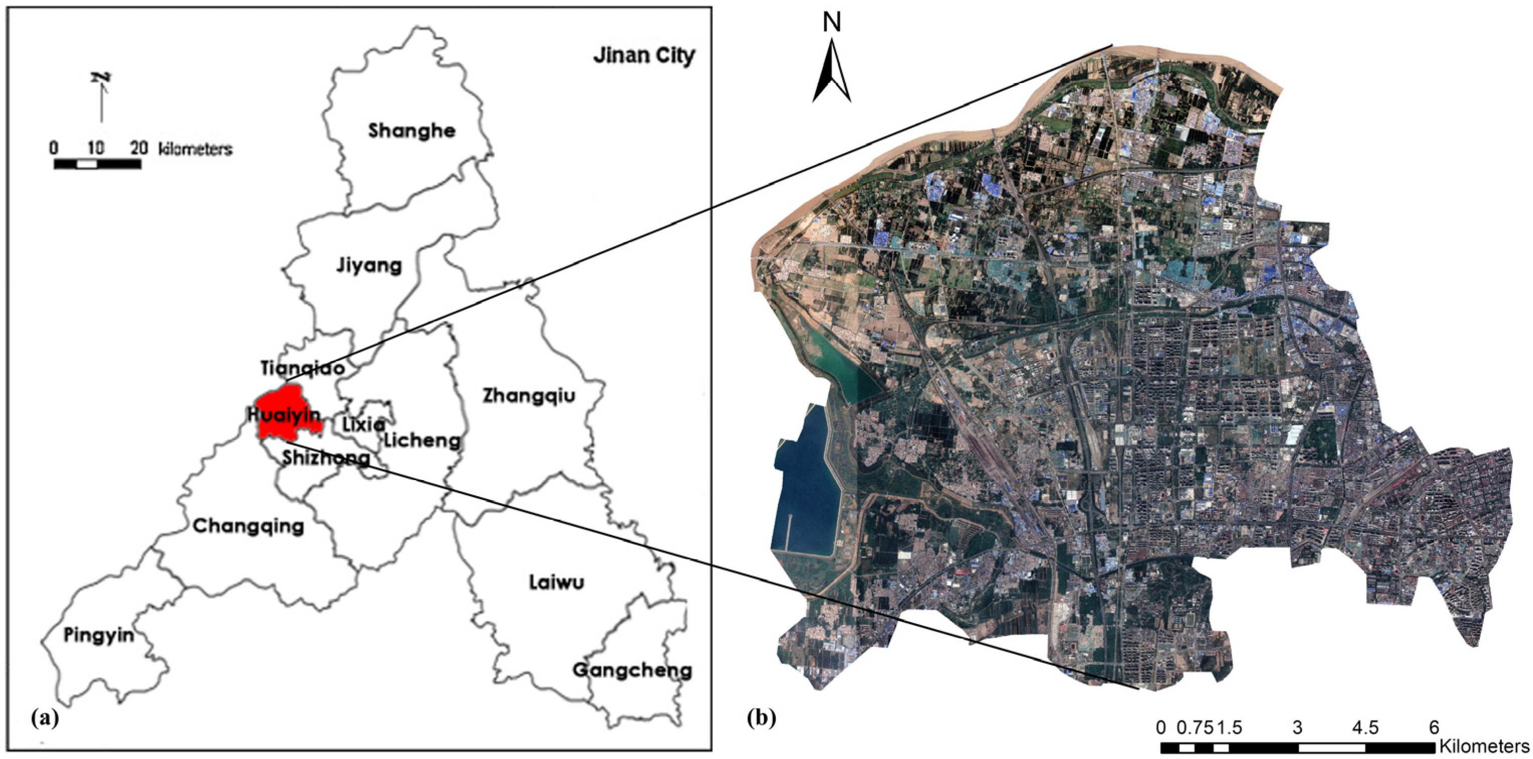
2.1. Study Area, Data Sources and Data Integration Method

(1) Study area

This research mainly analysed the LST spatial cluster characteristics in Huaiyin District, Jinan, China, to explore the change in the urban thermal environment. Based on the analysis of the LST spatial cluster areas in the Huaiyin area, this research provides a quantitative basis for the rational planning of urban spatial patterns and ecological quality improvement and provides a reference for other cities facing similar urban thermal environment problems. Jinan’s rapid urban expansion and its location in a valley topography mean the city cannot effectively dissipate heat to the surrounding areas, causing the city’s higher LST. Therefore, Jinan has become a high-temperature cluster area, with its all-time highest temperature reaching 44.7 °C. The Huaiyin District, located west of Jinan, is a key urban construction and development area. It has experienced the fastest growth in the city and the most significant change in the urban thermal environment. Due to rapid urban expansion, increasing population agglomeration and limited urban planning space, the Huaiyin District is severely affected by the heat island effect and has become a typical case in the research of LST spatial cluster characteristics.

The land coverage area of the Huaiyin District is 151.61 km² and includes three urban area types: the urban area, urban–rural fringe, and rural area [29] (Figure 1). The Huaiyin District, with its large land area and LST changes due to land-cover changes and development patterns, is an ideal location for this research. Analysing the LST spatial clustering in this study area can not only provide a quantitative basis for the rational planning of the urban spatial distribution and urban ecological quality improvement in the Huaiyin District of Jinan City but also provides reference and informative value for other cities facing similar urban thermal environment problems.

(2) Remote sensing data sources

The LST spatial distribution is a significant characteristic for evaluating the urban thermal environment. Therefore, analysing the LST spatial pattern and change process provides a basis for studying the urban thermal environment’s spatial pattern. As the LST is sufficiently sensitive to allow for identifying temporal and spatial differences in the thermal environment, exploring the change in the LST spatial distributions can effectively characterise the spatial and temporal changes in the urban thermal environment [28]. With the continual development of RS technology and LST retrieval algorithms, LST data obtained through RS monitoring have become an important data source for investigating the urban thermal environment’s spatial and temporal distribution characteristics. Consequently, RS monitoring can provide an accurate database for studying the LST spatial distribution and cluster characteristics [14].

This research quantitatively analysed the LST spatial cluster characteristics based on LST data, which was retrieved from the Landsat satellite thermal infrared data. Landsat satellite data are derived from the Earth observation satellite system launched by the National Aeronautics and Space Administration (NASA) and the United States Geological Survey (USGS) [30]. Landsat’s thermal infrared band is sensitive to the thermal radiation information of ground objects, and the surface radiation information received by the thermal infrared sensors of Landsat satellites can more accurately reflect the LST spatial distribution characteristics after retrieval and correction. Therefore, Landsat data have been widely used for monitoring LST changes [8]. Landsat images with no cloud cover and clear images in the study area were selected as the data source to accurately reflect the LST spatial distribution characteristics for similar time periods during the summers of 2000, 2005, 2010, 2015, 2020, and 2024 (

Table 1. Landsat data used in this research.

Acquisition Time	Satellite	Sensor
14 September 2000	Landsat 7	ETM+
15 May 2005	Landsat 5	TM
17 August 2010	Landsat 5	TM
12 June 2015	Landsat 8	OLI/TIRS
28 August 2020	Landsat 8	OLI/TIRS
20 June 2024	Landsat 8	OLI/TIRS

). These images were acquired from Landsats 5, 7, and 8, with a spatial resolution of 30 m and row and column numbers of 122/35. This research used the thermal infrared bands (Band 6 (10.40 μm to 12.50 μm) of Landsat 5 and Landsat 7; Band 10 (10.60 μm to 11.19 μm) of Landsat 8 and Landsat 9), red bands (Band 3 (0.63 μm to 0.69 μm) of Landsat 5 and Landsat 7; Band 4 (0.64 μm to 0.67 μm) of Landsat 8 and Landsat 9) and near-infrared bands (Band 4 (0.76 μm to 0.90 μm) of Landsat 5 and Landsat 7; Band 5 (0.85 μm to 0.88 μm) of Landsat 8 and Landsat 9) as the data sources. The original RS images were pre-processed with geometric correction and radiometric calibration. The images were cropped within the boundary of the Huaiyin District of Jinan City to obtain the RS image data for the study area.

(3) Spatial grid statistical method

The Landsat satellite data from different periods exhibit different spatial parameters, including different spatial resolutions and spatial coordinate systems. Therefore, this research established a geographic information grid to integrate all the data through the ArcGIS platform. Min et al. [31] showed that the 300 m scale is suitable for studying the LST spatial distribution characteristics. Therefore, the 300 m scale geographic information grid was used for data integration in this research to improve the LST data accuracy. The spatial analysis tools in ArcGIS were used to integrate all the layers into a geographic information grid at the same scale. The values that corresponded to larger units in the geographic information grids were obtained by calculating the mean value among the pixels in the raster data layers within the extent of the larger unit, and the values that corresponded to smaller units were obtained through interpolation calculations performed with the original raster data.

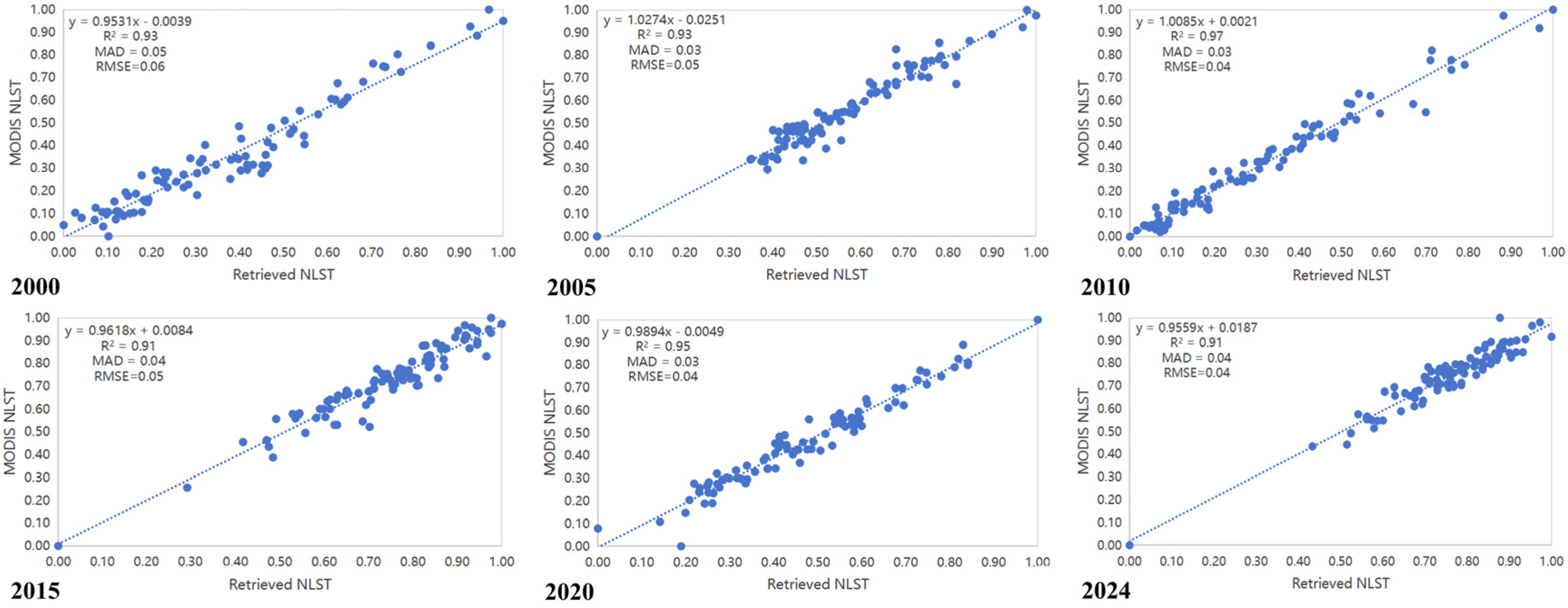
2.2. Land Surface Temperature Retrieval Method Based on Radiative Transfer Equation

There are three commonly used LST retrieval methods, namely, the RTE, single-window algorithm [32], and split-window algorithm [33], among which the RTE has been widely used due to its simplicity, universality, and small simulation error [34]. Therefore, this research used the RTE method to retrieve the LST from RS images on the ArcGIS platform.

Planck’s law (blackbody radiation law) describes the correlation between the intensity and wavelength of an object’s radiation and its temperature. Furthermore, the LST can be retrieved with an inverse function based on this correlation [35]. Radiation energy is attenuated as it travels through a medium because of absorption and scattering by the medium. RTE can eliminate the influence of the atmospheric medium on thermal radiation during radiation transfer based on the real-time atmospheric data acquired so that satellite infrared data can more accurately retrieve the LST [36]. The RTE method applies to all thermal infrared data from Landsat satellites and can accurately retrieve the LST based on different periods of historical data from each Landsat satellite [37].

The LST ($t_i$) is calculated according to Planck’s formula as follows [38]:

$$t_i={\displaystyle \frac{K_2}{\mathit{ln}\left[\left(K_1/L_i\right)+1\right]}}-K_3$$

(1)

where $K_1$ (unit: W/(m²·sr·μm)) and $K_2$ (unit: W) are calibration constants defined for the Landsat satellites ($K_1$ = 607.76 W/(m²·sr·μm) and $K_2$ = 1260.56 W for Landsat 5; $K_1$ = 666.09 W/(m²·sr·μm) and $K_2$ = 1282.71 W for Landsat 7; $K_1$ = 774.89 W/(m²·sr·μm) and $K_2$ = 1321.08 W for Landsat 8), $K_3$ is a constant used to convert the unit from kelvin to degrees Celsius and is approximately 273, and $L_i$ is the radiation brightness of the thermal band for the spatial unit $i$. In this research, $L_i$ was converted from the radiation values of the thermal infrared band images observed by the Landsat satellites. Since the atmospheric conditions significantly affect the radiation values obtained from satellite sensor observations [39], this research used the RTE method to convert the radiation values to radiation brightness to resolve the atmospheric effects in the LST retrieval as follows:

$$L_i=({\lambda }_i-L_{\mathit{up}}-\tau \times \left(1-{\epsilon }_i\right)\times L_{\mathit{down}})/(\tau \times {\epsilon }_i)$$

(2)

where $L_{\mathit{down}},L_{\mathit{up}} \mathrm{and} \tau$ are the satellite-observed atmospheric parameters representing the atmospheric downwelling and upwelling radiances and the atmospheric transmission, respectively; ${\lambda }_i$ is the radiation value in the Landsat thermal band for spatial unit $i$; ${\epsilon }_i$ is the land surface emissivity for spatial unit $i$, which is estimated using the normalised difference vegetation index (NDVI) threshold method with the NDVI data derived from the Landsat spectral data as follows [40]:

$${\epsilon }_i=K_4\times {\displaystyle \frac{\left(\frac{N_i-R_i}{N_i+R_i}\right)-\mathit{min}\left(\frac{N_i-R_i}{N_i+R_i}\right)}{\mathit{max}\left(\frac{N_i-R_i}{N_i+R_i}\right)-\mathit{min}\left(\frac{N_i-R_i}{N_i+R_i}\right)}}+K_5$$

(3)

where $K_4$ and $K_5$ are the land surface emissivity constants, with values of approximately 0.004 and 0.9886, respectively, and $N_i$ and $R_i$ are the near-infrared band and red band values for the spatial unit $i$, respectively. $N_i$ and $R_i$ are obtained from the corresponding band data of Landsat satellites using radiometric calibration. Radiometric calibration refers to converting the digital number (DN) value (0~255) of a digitised thermal infrared sensor into radiation values with practical significance. Before retrieving the LST, the DNs from the thermal infrared band must be converted to radiation values. For Landsat satellites, the radiometric calibration formula for the radiation value (${\epsilon }_i$) in Equation (2) is as follows:

$${\lambda }_i=G_b\times D_i+D_b$$

(4)

where $D_i$ is the Landsat dimensionless digital number measured using the sensor for spatial unit i, $G_b\mathrm{and}{D}_b$ are the gain value ($\mathrm{W}/({\mathrm{m}}^2·\mathrm{s}\mathrm{r}·\mathsf{\mu }\mathrm{m})$) and deviation value ($\mathrm{W}/({\mathrm{m}}^2·\mathrm{s}\mathrm{r}·\mathsf{\mu }\mathrm{m})$) for band b of the Landsat satellites, respectively, and they are provided in the RS satellite data files.

The LST calculated from the retrieval formula can characterise the LST at a specific date. Still, this is unsuitable for the comparative analysis of LST and cluster characteristics at different times due to differences in the climatic environments. This is because differences in climatic environments impact the absolute LST values but not the distribution patterns. In this research, the normalised land surface temperature ($T_i$) was used to explain the LST spatial distribution pattern to ensure the comparability of the LST values retrieved from satellite images at different times [41]; its formula is as follows:

$$T_i={\displaystyle \frac{t_i-\mathit{min}\left(t_i\right)}{\mathit{max}\left(t_i\right)-\mathit{min}\left(t_i\right)}}$$

(5)

where $\mathit{min}\left(t_i\right)$ and $\mathit{max}\left(t_i\right)$ are the minimum and maximum values of all the LST values, respectively.

The LST spatial distribution characteristics could be quantitatively identified by comparing the spatial distribution of the normalised land surface temperatures in the images on the ArcGIS platform.

To check the retrieved normalised land surface temperature accuracy, MODIS LST 1 km remote sensing data [42] within the same period were obtained as validation data in this study. A 1 km × 1 km grid was created in ArcGIS using the Fishnet tool, and the mean normalised land surface temperature values in each area were compared with the MODIS LST values for validation. The spatial distributions of the normalised land surface temperature and MODIS LST in the study area were relatively consistent. Therefore, it was considered that the normalised land surface temperature results from Landsat images were representative and could be used to characterise the LST spatial cluster characteristics in Huaiyin District. This study compared normalised land surface temperature with MODIS LST products using mean absolute differences (MAD), root mean square error (RMSE), and R² as quantitative evaluation criteria [37].

2.3. Identification of LST Spatial Cluster Areas

Under the effect of convective heat transfer in urban spaces, the LSTs in neighbouring spaces interact with each other, leading to LST spatial cluster areas. In the study of LST, local Moran’s I serves as a valuable tool for assessing the clustering or dispersion patterns of temperature data across a study area and the intensity and significance of these trends. By analysing the local Moran’s I, this research gained insight into the LST spatial cluster characteristics, identifying areas where high temperatures clustered together and regions where low temperatures formed distinct patterns. This research used the spatial cluster area classification of the local Moran’s I to classify the LST spatial cluster areas [43], leading to three types of LST spatial cluster areas: LL, HH and NO [44]. Unlike traditional LST classification methods, the spatial cluster area classification method used in this research quantitatively identified the LST spatial cluster characteristics using LST spatial cluster areas, which reflected not only the relationship between an area and the entire study area but also the cluster degree and area range of the LST.

(1) Spatial cluster test based on global Moran’s I

An LST spatial cluster is a concentration of LSTs with similar attributes in the area and the spatial distribution status of the LST spatial cluster area formed by these LSTs. In this research, the global Moran’s I was used to examine the spatial clustering of the LST data before the application of the local Moran’s I to classify the LST spatial cluster areas. The global Moran’s I test was used to ascertain the presence of spatial clusters in the LST spatial distribution. This was achieved by measuring the cluster areas’ status compared with the entire geographic unit space and the neighbouring spaces. The formula for the global Moran’s I ($I_G$) is expressed as follows [45]:

$$I_G={\displaystyle \frac{n}{{\Sigma }_{i=1}^n{\Sigma }_{j=1}^n{W}_{ij}}}\times {\displaystyle \frac{{\Sigma }_{i=1}^n{\Sigma }_{j=1}^n{W}_{ij}\left(t_i-\overline{t}\right)\left(t_j-\overline{t}\right)}{{\Sigma }_{i=1}^n{\left(t_i-\overline{t}\right)}^2}}$$

(6)

where $t_j$ is the LST at spatial unit j, which is adjacent to spatial unit i; $\overline{t}$ is the average LST value; n is the total number of spatial units; $W_{ij}$ is the spatial weight between spatial units i and j; and ${\Sigma }_{i=1}^n{\Sigma }_{j=1}^n{W}_{ij}$ is the sum of all spatial weights.

(2) Spatial cluster area classification based on local Moran’s I

Following the confirmation of the LST values’ spatial clustering, the spatial cluster area classification of the local Moran’s I was used to classify the LST spatial cluster areas, namely, the HH, LL, and NO areas. The formula for calculating the local Moran’s I ($I_i$) is as follows [46]:

$$I_i={\displaystyle \frac{t_i-\overline{t}}{l^2}}\times {\sum }_{k=1,k\ne i}^{n-1}\left[w_{ik}\left(t_k-\overline{t}\right)\right]$$

(7)

where $t_k$ is the LST at spatial unit k (which is a spatial unit that is not unit i), $w_{ik}$ is a weight value related to the distance between spatial units i and k and ranges within [−1, 1], and $l^2$ is the variance of the variable Z given by

$$l^2={\displaystyle \frac{{\sum }_{i=1}^n{(t_i-\overline{t})}^2}{n}}$$

(8)

In summary, as shown in Equation (7), $I_i$ is dependent on ${\displaystyle \frac{t_i-\overline{t}}{l^2}}$ and ${\sum }_{k=1,k\ne i}^{n-1}\left[w_{ik}\left(t_k-\overline{t}\right)\right]$. ${\displaystyle \frac{t_i-\overline{t}}{l^2}}$ represents the strength of the relationship between the LST of unit i and the entire study area’s average LST. In contrast, ${\sum }_{k=1,k\ne i}^{n-1}\left[w_{ik}\left(t_k-\overline{t}\right)\right]$ represents the strength of the relationship between the LST of the spatial unit i and the neighbouring area’s average LST. The LST spatial cluster area of unit i can be classified by comparing the positive and negative values of ${\displaystyle \frac{t_i-\overline{t}}{l^2}}$ and ${\sum }_{k=1,k\ne i}^{n-1}\left[w_{ik}\left(t_k-\overline{t}\right)\right]$ in $I_i$ for different areas, with the determination criteria shown in

Table 2. Determination criteria for cluster areas.

LST Spatial Cluster Area	$\frac{{\mathit{t}}_{\mathit{i}}-\overline{\mathit{t}}}{{\mathit{l}}^2}$	${\sum }_{\mathit{k}=1,\mathit{k}\ne \mathbf{i}}^{\mathit{n}-1}\left[{\mathit{w}}_{\mathit{i}\mathit{k}}\left({\mathit{t}}_{\mathit{k}}-\overline{\mathit{t}}\right)\right]$	Meaning
HH area	>0	>0	The LST of the spatial unit i is high, and its neighbouring LST is high.
LL area	<0	<0	The LST of the spatial unit i is low, and its neighbouring LST is low.
NO area	<0	>0	The LST of the spatial unit i is not similar to its neighbouring LST.
	>0	<0

.

2.4. LST Spatial Cluster Characteristics Analysis

(1) Spatial barycentre

The spatial barycentre is the location index of spatial elements, and its transfer reflects the spatial distribution trend of spatial elements. The spatial barycentres of the LST spatial cluster area types in different periods reflect the change in the LST spatial cluster characteristics. If a specific LST spatial cluster area type maintains a uniform increase or decrease in all spatial orientations, its spatial barycentre remains unchanged. If there is an obvious increase or decrease in a specific direction, the spatial barycentre of the LST spatial cluster area type changes significantly [47].

In this research, the spatial barycentres of the LST spatial cluster area types were obtained based on a spatial barycentre transfer to reveal the spatial change characteristics of the urban thermal environment. The specific formula used to calculate the barycentric coordinates ($X_{\mathit{tp}}$,$Y_{\mathit{tp}}$) of LST spatial cluster area type p in year t is expressed as follows:

$$X_{\mathit{tp}}={\displaystyle \frac{{\sum }_{r=1}^{n_{\mathit{tp}}}{X}_{\mathit{tpr}}}{n_{\mathit{tp}}}}$$

(9)

$$Y_{\mathit{tp}}={\displaystyle \frac{{\sum }_{r=1}^{n_{\mathit{tp}}}{Y}_{\mathit{tpr}}}{n_{\mathit{tp}}}}$$

(10)

where $n_{\mathit{tp}}$ is the number of units in LST spatial cluster area type p in year t, and $X_{\mathit{tpi}}$ and $Y_{\mathit{tpi}}$ are the horizontal and vertical coordinates of the geometric centre of spatial unit i of LST spatial cluster type p in year t, respectively.

(2) Spatial pattern index

To compare the spatial shape and scale of the LST spatial cluster area types in different periods, this research used landscape indexes to characterise the spatial pattern of the LST spatial cluster characteristics. The landscape index is a mathematical analysis method for quantitatively characterising the spatial pattern of different patches [48]. This study examined the LST spatial cluster characteristics in terms of the area, shape, and aggregation and these results were combined with the ecological significance of landscape indexes [49,50]. The landscape indexes selected for this study were the percentage of landscape (PLAND), which represents the landscape area, the landscape shape index (SHAPE), which represents the numbers and sizes of different area types, and the aggregation index (AI), which represents the shape complexities of different area types and spatial aggregation trends of different area types.

The PLAND is the areal proportion occupied by each LST spatial cluster area type. The formula for PLAND is as follows:

$$\mathit{PLAND}={\displaystyle \frac{{\sum }_{r=1}^m{a}_{\mathit{rp}}}{A}}$$

(11)

where $a_{\mathit{rp}}$ is the area (m²) of patch r in LST spatial cluster area type p, m is the number of type p patches in the spatial unit, and A is the total study area (m²).

The SHAPE measures the average shape of each LST spatial cluster area type patch within a spatial unit. By comparing the perimeter and area of the patches, it is possible to intuitively reflect the shape complexity of each LST spatial cluster area type patch and its deviation from an equal-area rectangle. The SHAPE value ranges from 1 to ∞. When the SHAPE is equal to 1, the shape of the LST spatial cluster area type patch is a square. As the shape of the LST spatial cluster area type patch becomes increasingly irregular, the SHAPE increases. The formula for the SHAPE is as follows:

$$\mathit{SHAPE}={\displaystyle \frac{0.25{\sum }_{r=1}^m{P}_{\mathit{rp}}}{\sqrt{{\sum }_{r=1}^m{a}_{\mathit{rp}}}}}$$

(12)

where $P_{\mathit{rp}}$ is the edge length (m) of patch r in LST spatial cluster area type p.

The AI represents the adjacency relationship between patches of the same LST spatial cluster area type. When the AI is maximised, the common boundary of all spatial units in the LST spatial cluster area type reaches the maximum value; that is, the cluster degree in the LST spatial cluster area type is the highest. The formula for the AI is as follows:

$$\mathit{AI}={\displaystyle \frac{g_p}{\mathit{max}\to g_p}}$$

(13)

where $g_p$ is the number of like adjacencies between spatial units of LST spatial cluster area type p, and $\mathit{max}\to g_p$ is the maximum number of like adjacencies between the spatial units of LST spatial cluster area type p (maximum possible number of like adjacencies of type p when type p is maximally clumped into a single patch).

3. Results

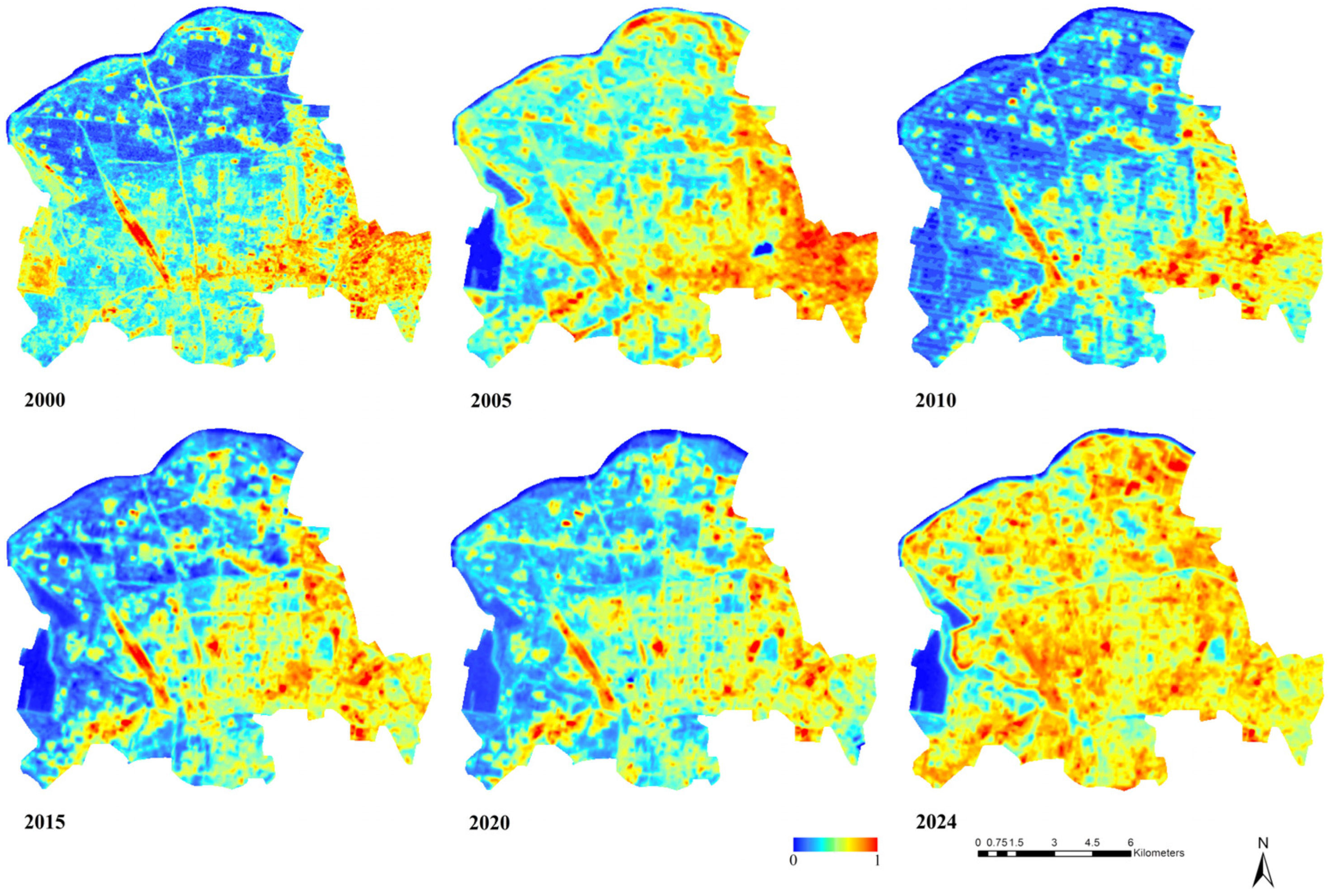
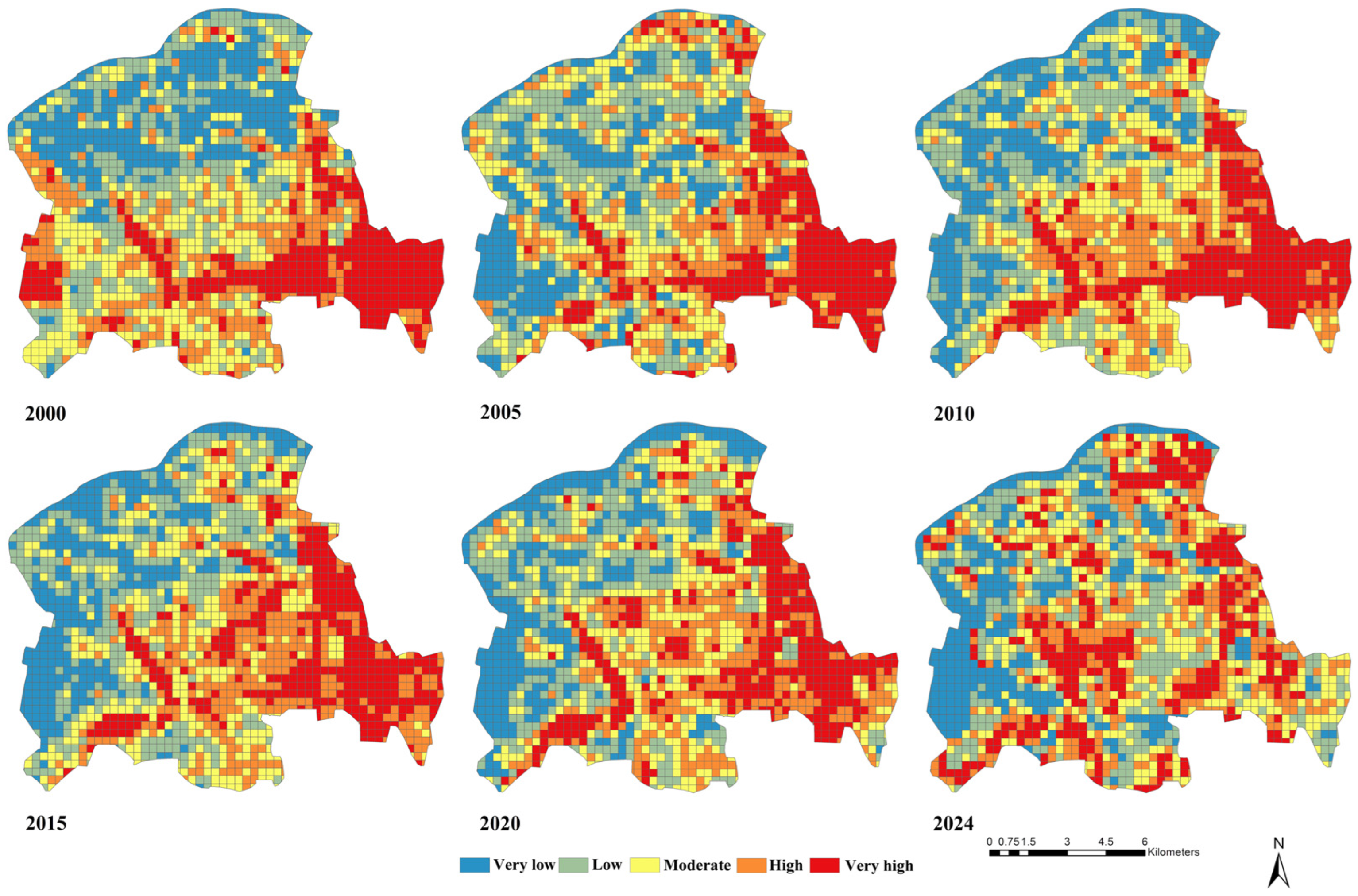
3.1. LST Spatial Distribution

To avoid the situation where different times and seasons lead to different urban values in different periods that cannot be directly compared, this research used the normalised land surface temperature to study the LST spatial distribution [41]. Due to urban development and spatial structure changes, the normalised land surface temperature showed a significant change in trend. Figure 2 shows the spatial distribution map of the normalised land surface temperatures in 2000, 2005, 2010, 2015, 2020, and 2024.

In this study, the retrieved normalised land surface temperatures were compared with the normalised MODIS LST products to obtain a scatter plot and validate the accuracy of the data. Figure 3 shows the validation results between the retrieved normalised land surface temperatures (Retrieved NLST) and the normalised MODIS LST products (MODIS NLST). The plot shows a good fit (R² ≥ 0.91, MAD ≤ 0.05 and RMSE ≤ 0.06) of calculated normalised land surface temperatures.

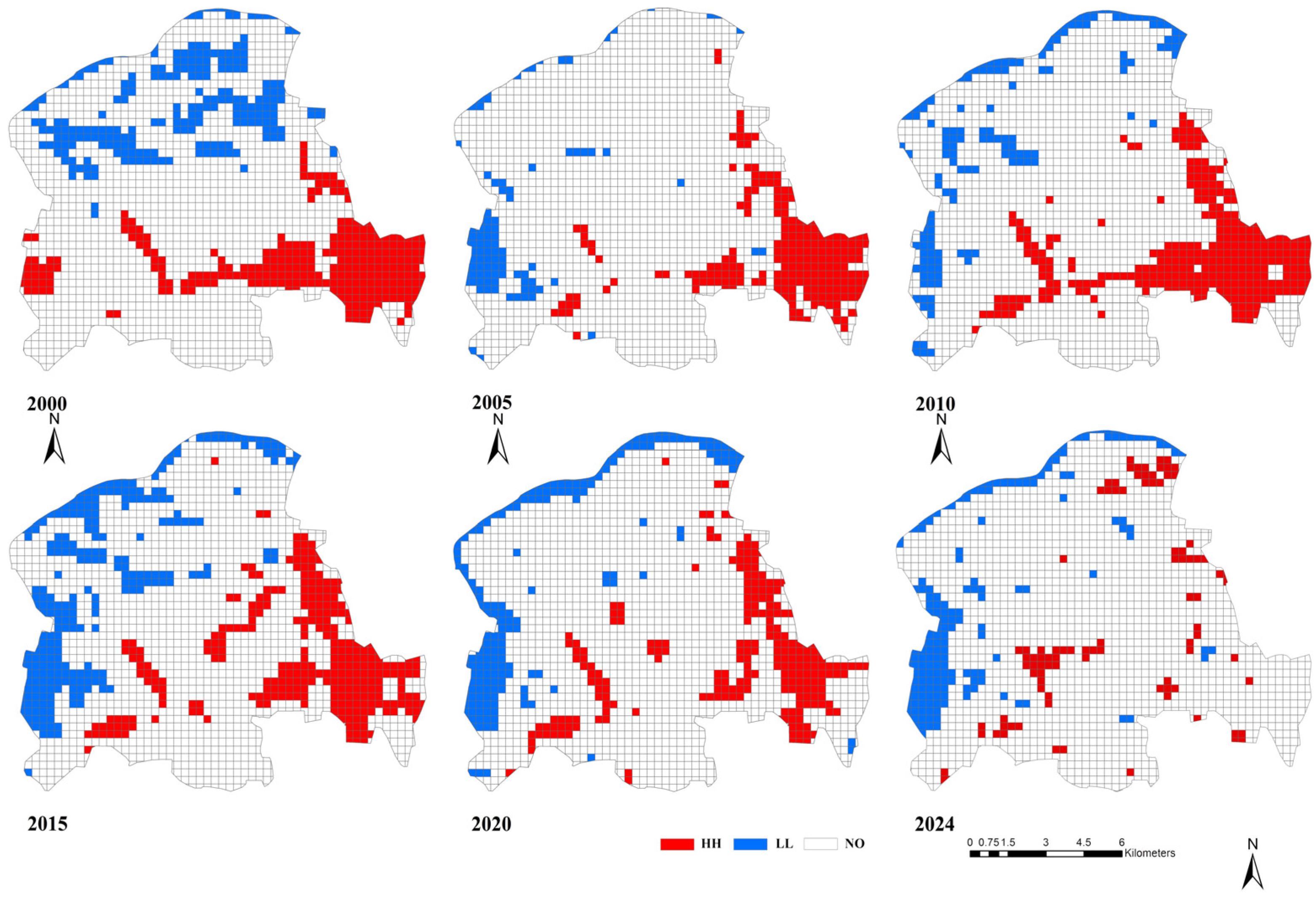
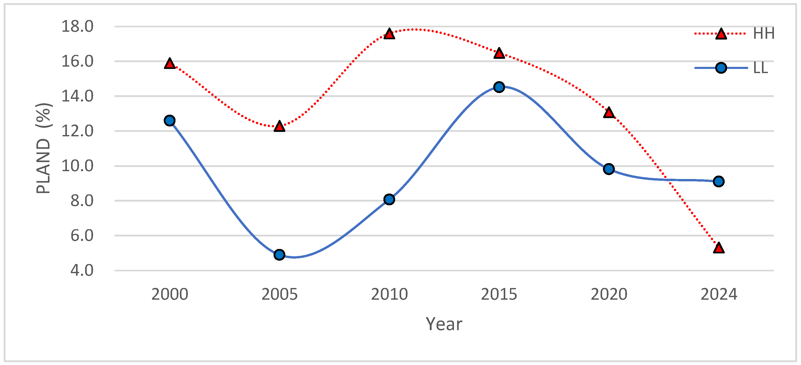
3.2. LST Spatial Cluster Area

In addition, based on the normalised land surface temperature results, the global Moran’s I was used to test the LST spatial cluster characteristics in geographic space, as shown in

Table 3. Global Moran’s I coefficients of LST.

Time	2000	2005	2010	2015	2020	2024
Global Moran’s I	0.75	0.56	0.78	0.79	0.72	0.73
Z score	44.1	32.9	46.3	46.7	42.7	42.9
p value	0	0	0	0	0	0

. The results show that the global Moran’s I values ranged from 0.56 to 0.79 in 2000, 2005, 2010, 2015, 2020, and 2024. The global Moran’s I values were positive in all years, with high Z scores and p values of 0, indicating that the LST showed significant spatial cluster characteristics in Huaiyin District, Jinan City.

According to the time series of the global Moran’s I (Figure 4), the LST in 2005 was relatively dispersed (global Moran’s I < 0.7), while the LST spatial distributions in other years were relatively clustered (0.7 ≤ global Moran’s I).

After verifying the LST spatial cluster characteristics, this study explored the LST spatial cluster characteristics using the local Moran’s I’s spatial cluster area classification. Figure 5 shows the LST spatial cluster areas in 2000, 2005, 2010, 2015, 2020, and 2024. The LST in this study area presented three LST spatial cluster area types: HH, LL, and NO. The HH area had a high LST and showed clustering with other high LSTs, and the LL area had a low LST and showed clustering with other low LSTs. The LST dataset exhibited a distinct separation between the HH and LL areas. The spatial distributions of the HH and LL areas contrasted from north to south and west to east.

Compared with the direct classification results (Figure 6), the spatial cluster area classification based on local Moran’s I (Figure 5) used in this study offers clear advantages in identifying HH and LL areas within the study area. This method more accurately reflects the spatial autocorrelation of LST and provides more meaningful spatial classifications. Firstly, direct classification methods rely on fixed numerical temperature thresholds, which makes it challenging to distinguish between isolated high-temperature points (such as scattered high or very high-temperature spots in the northwest) and extensive high-temperature regions (such as the widespread high or very high-temperature areas in the southeast). In contrast, our method employs a spatial weight matrix that enhances the identification of local LST anomalies, effectively reducing the occurrence of isolated high-temperature points caused by minor fluctuations and is more suitable for analysing LST spatial patterns at urban or regional scales. Secondly, direct classification results are susceptible to numerical noise, which can lead to the misclassification of randomly distributed high/low-temperature points as significant HH/LL areas (such as randomly occurring high or very high-temperature points in the centre). By incorporating a statistical significance test (e.g., p value), our method filters out random noise and retains only statistically significant clusters, thereby greatly reducing misclassifications due to randomness and enhancing the reliability of the results. Thirdly, while direct classification solely relies on temperature thresholds, ignoring the interactions and dependencies between spatial neighbours, our method analyses the correlation between each spatial unit and its neighbours. This enables the identification of LST spatial cluster patterns and produces more coherent temperature clusters that reflect the true spatial continuity of geographic phenomena. In summary, by integrating spatial autocorrelation analysis, statistical testing, and neighbourhood relationship modelling, the local Moran’s I’s spatial cluster area classification provides a more scientific and robust way to reveal the spatial patterns of high/low LST regions. It not only uncovers the spatial dependence and heterogeneity of surface temperature but also effectively identifies spatial cluster characteristics. In contrast, while the direct classification method is straightforward and intuitive, its reliance on fixed numerical thresholds limits its ability to capture spatial correlations and statistical significance, potentially overlooking critical spatial pattern information.

Table 4. LST spatial cluster areas.

	2000	2005	2010	2015	2020	2024
HH area (km2)	24.04	18.68	26.73	25	19.84	8.23
LL area (km2)	19.07	7.43	12.24	22.01	14.88	14.12
NO area (km2)	108.50	125.5	112.63	104.6	116.89	132.26

shows that the spatial distribution of the NO areas in the Huaiyin District of Jinan City was extensive, where it ranged from 104.6 km² to 132.26 km². The total HH area showed a fluctuating pattern, where it ranged from 18.68 km² to 26.73 km². There were also significant changes in the spatial pattern of the HH areas (Figure 5). The HH areas were mainly located in the Jixi National Wetland Park (when under construction), the newly built urban growth area and the old urban area, which covered large areas of impervious surfaces and contained numerous residential buildings and roads.

Table 4 also shows that the LL areas ranged from 7.43 km² to 22.01 km². With urban development, there were obvious changes in the spatial pattern of the LL areas, which were mainly located in the Jixi National Wetland Park and the northern part of the study area; these areas were mostly covered by vegetation or water bodies and had lower LSTs (Figure 5).

The spatial distributions of the HH and LL areas changed significantly over time. Overall, the total area of the HH and LL areas showed a decreasing trend in 2000, 2005, 2010, 2015, 2020, and 2024. The HH areas were mainly located in urban built-up areas, such as the old urban area; the LL areas were mainly located in suburban areas with large areas of vegetation and water bodies, such as the Jixi National Wetland Park and Yellow River basin.

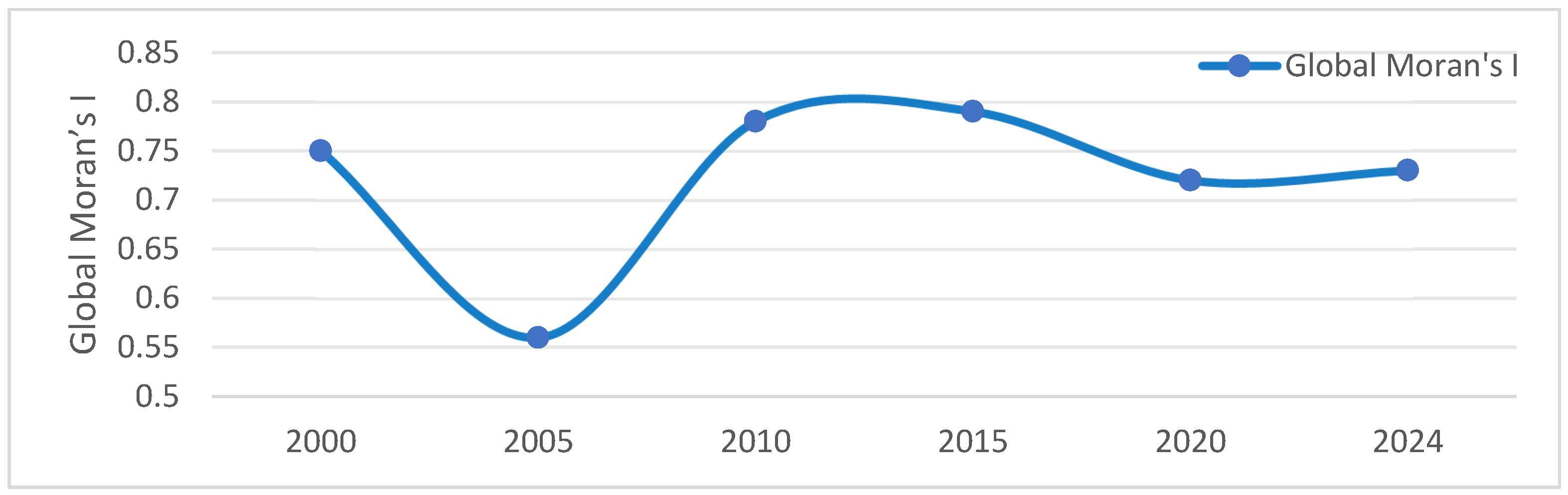
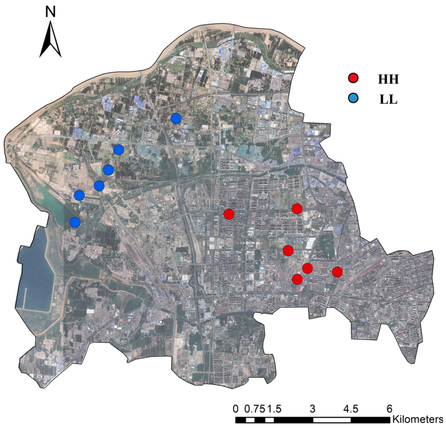
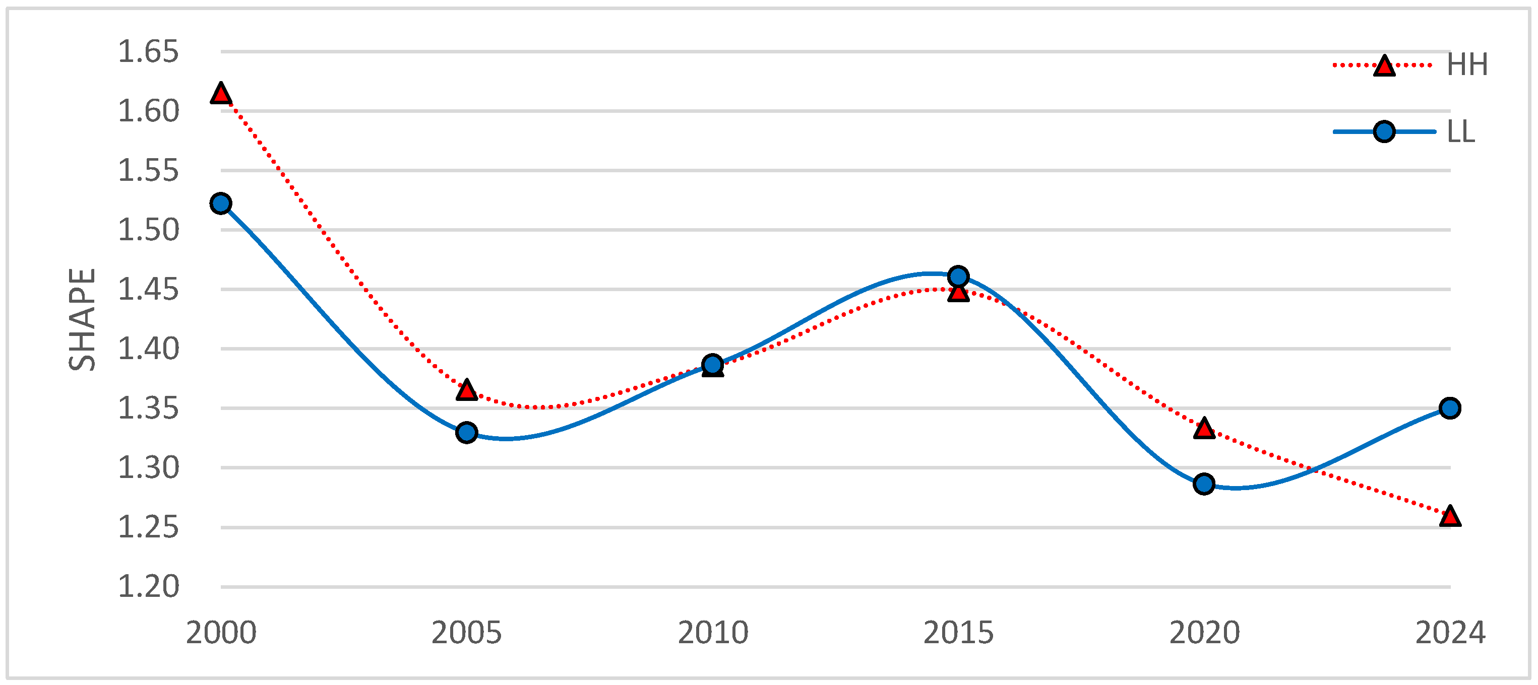
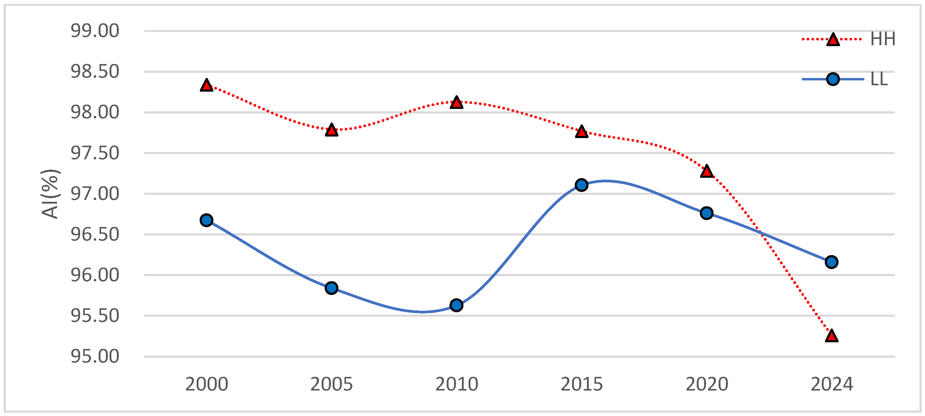
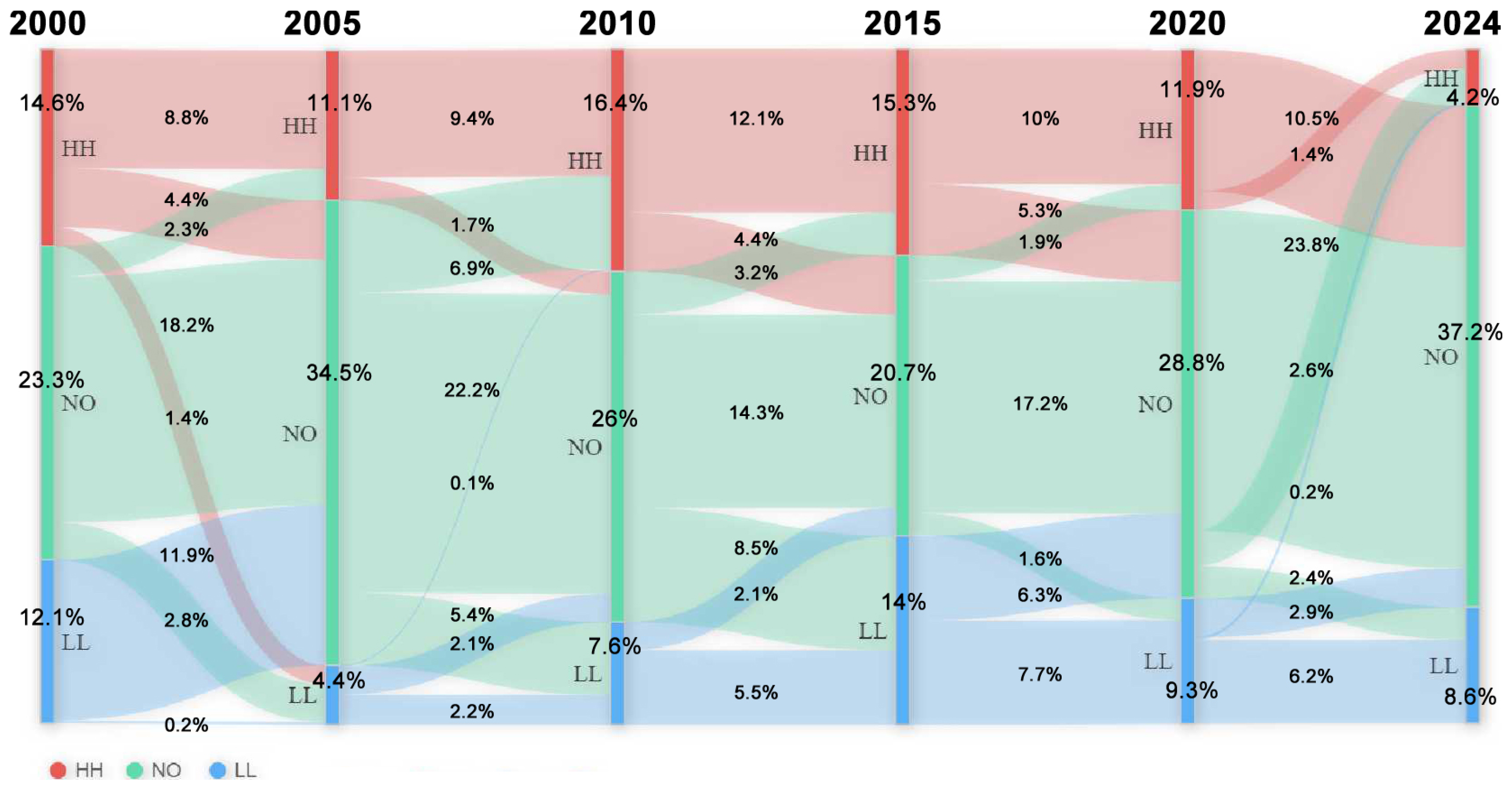
3.3. LST Spatial Cluster Characteristics

(1) Spatial distribution of spatial barycentre

The LST spatial cluster area data from 2000, 2005, 2010, 2015, 2020, and 2024 were selected to calculate the spatial barycentre of the LST spatial cluster area for each year (Figure 7). The HH area spatial barycentre was located in the southeastern urban built-up area, and the LL area spatial barycentre was located in the northwestern vegetation and water body covered area. During the research period, the transfer of the spatial barycentre of the HH areas was closely related to the expansion of urban built-up areas, while the transfer of the spatial barycentre of the LL areas was closely related to the contraction of the peri-urban vegetation and water bodies.

(2) Spatial pattern

The PLAND, SHAPE, and AI reflected the spatial patterns of the number, shape, and structure of the LST spatial cluster areas. The PLAND values primarily indicate the percentage of the total area covered by the different types of LST cluster patches. A higher PLAND value indicates a larger area of different LST cluster patches. Figure 8 shows that many PLAND values in the HH area were lower than in the LL area in 2000, 2005, 2010, 2015, 2020, and 2024, indicating that many HH areas had larger patch sizes than the LL areas. This result was probably due to the gradual increase in the built-up area, which made the patch size of the HH area generally larger than that of the LL area.

The SHAPE values mainly reflected the patch shape in the different LST spatial cluster areas. Higher SHAPE values show more complex shapes of different LST spatial cluster areas. The SHAPE values of the HH and LL areas show obvious fluctuations (Figure 9). This indicates that the patch shape complexity of the HH and LL areas showed irregular changes.

The AI values mainly reflect the concentration degree of the different patches of LST spatial cluster areas. Higher AI values imply a greater neighbourhood of different LST spatial cluster areas. Figure 10 shows that the HH area AI values were generally higher than those of the LL area in 2000, 2005, 2010, 2015, 2020, and 2024. This indicates that the patches in the HH area were generally more concentrated than those in the LL area. It is important to note that the spatial distributions of the HH and LL areas during the study period were relatively concentrated (AI > 95%).

Overall, there were significant changes in the PLAND, SHAPE, and AI in 2000, 2005, 2010, 2015, 2020, and 2024 for the HH and LL areas. The HH area exhibited a gentler trend than the LL area. Compared with the LL areas, the HH areas were larger, simpler in patch shape and more aggregated in spatial distribution.

4. Discussion

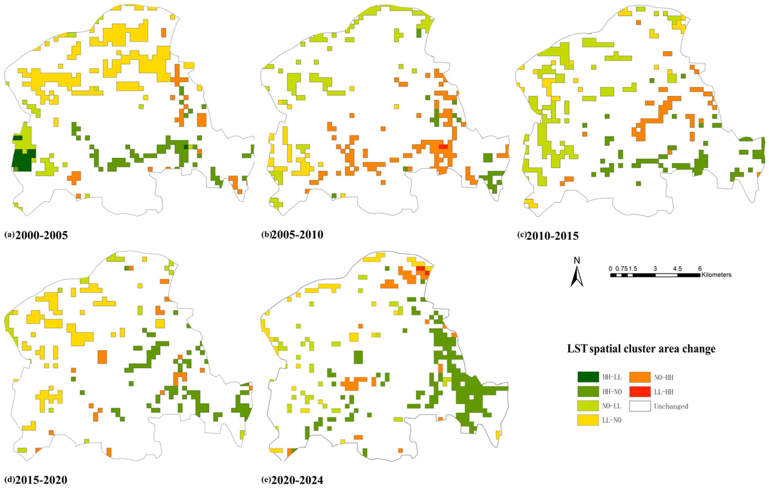
4.1. Spatial Distribution of LST Spatial Cluster Areas

In terms of the spatial pattern, the HH areas changed significantly. With urban expansion, the urban HH areas increased the patch shape complexity, decreased the patch concentration degree, and increased the fragmentation degree. These findings are consistent with those of Peng et al. [51]. Furthermore, the spatial barycentre transfer of the HH and LL areas was affected by the expansion of built-up areas and the contraction of suburban vegetation and water bodies, respectively, and the spatial barycentre distribution was closely related to urban development planning, which is similar to the study by Liu et al. [52].

This study found significant characteristics in the spatial distribution of the LST cluster areas. We overlaid the LST cluster areas at different times to investigate the urban cluster characteristics. The transfer maps of the LST spatial cluster areas, which were analysed by overlaying the LST cluster areas over many years, revealed the transfer patterns between different LST spatial cluster area types [53]. The study area presented seven types of LST spatial cluster area transfer in the transfer maps, namely, low-temperature cluster areas transferred to high-temperature cluster areas (LL-HH), low-temperature cluster areas transferred to not obvious areas (LL-NO), not obvious areas transferred to high-temperature cluster areas (NO-HH), high-temperature cluster areas transferred to low-temperature cluster areas (HH-LL), high-temperature cluster areas transferred to not obvious areas (HH-NO), not obvious areas transferred to low-temperature cluster areas (NO-LL), and unchanged areas (Unchanged) (including HH-HH, NO-NO, and LL-LL). Using the transfer map, this research analysed the spatial distribution data of the LST spatial cluster areas and obtained a Sankey map of the LST spatial cluster area transfers in 2000, 2005, 2010, 2015, 2020, and 2024 (Figure 11). Among them, 50% of the study area transferred from 2000 to 2024, which comprised approximately one-quarter of both the HH and LL areas and around half of the NO areas. From 2000 to 2005, the increasing temperature transformation involved the NO-HH and LL-NO areas, which accounted for 2.3% and 11.9% of the study area. The decreasing temperature transformations involved the HH-LL, HH-NO, and NO-LL areas, which accounted for 4.4%, 1.4%, and 2.8% of the study area, respectively. From 2005 to 2010, the increasing temperature transformation involved the NO-HH, LL-NO, and LL-HH areas, which accounted for 6.9%, 2.1%, and 0.1% of the study area, respectively. The decreasing temperature transformations involved the HH-NO and NO-LL areas, which accounted for 1.7% and 5.4% of the study area. From 2010 to 2015, the increasing temperature transformation involved the NO-HH and LL-NO areas, which accounted for 3.2% and 2.1% of the study area. The decreasing temperature transformations involved the HH-NO and NO-LL areas accounted for 4.4% and 8.5% of the study area. From 2015 to 2020, the increasing temperature transformation involved the NO-HH and LL-NO areas accounted for 1.9% and 6.3% of the study area. The decreasing temperature transformations involved the HH-NO and NO-LL areas accounted for 5.3% and 1.6% of the study area. From 2020 to 2024, the increasing temperature transformation involved the NO-HH, LL-HH, and LL-NO areas accounted for 1.4%, 0.2%, and 2.9% of the study area. The decreasing temperature transformations involved the HH-NO and NO-LL areas accounted for 10.5% and 2.4% of the study area. During the period of 2000–2010, the increasing temperature changes were greater than the decreasing temperature changes, which worsened the thermal environment. During the period of 2010–2024, the decreasing temperature transformations were more significant than the increasing temperature transformations, so the thermal environment generally provided relief. Half of the study area transferred from the HH, NO, and LL types to others from 2000 to 2024. Meanwhile, the HH, NO, and LL areas transferred from 14.6%, 23.3% and 12.1% of the total area to 4.2%, 37.2%, and 8.6% from 2000 to 2024, respectively. Overall, the changes in the thermal environment were complex from 2000 to 2024 and presented a “Deterioration—Relief” pattern.

Intersecting and overlaying the LST spatial cluster area maps for the years 2000, 2005, 2010, 2015, 2020, and 2024 resulted in five transfer maps (Figure 12), which illustrate the temperature transformations across the LST spatial cluster area. The trajectory lines of different colours indicate the transition from one LST spatial cluster area to another type during a specific time. The trajectory line thickness represents the conversion amount, with thicker lines indicating larger conversion amounts. From 2000 to 2005, the thermal environment transfer trends were as follows (Figure 12a): (1) The northern area of the study area showed increasing temperature transformations, namely, NO-HH and LL-NO. (2) The southern area of the study area showed decreasing temperature transformations, namely, HH-LL, HH-NO, and NO-LL. From 2005 to 2010, the thermal environment transfer trends were as follows (Figure 12b): (1) The western and northern areas of the study area showed decreasing temperature transformations, namely, HH-NO and NO-LL. (2) The southern and eastern areas of the study area showed overall increasing temperature transformations, namely, LL-NO, NO-HH, and LL-HH. (3) The southeastern area of the study area showed significantly decreasing temperatures, namely, HH-LL. From 2010 to 2015, the thermal environment transfer trends were as follows (Figure 12c): (1) The northern, western, and southern areas of the study area experienced decreasing temperature transformations, namely, HH-NO and NO-LL. (2) The western area of the study area showed increasing temperature transformations, namely, LL-NO and NO-HH. From 2015 to 2020, the thermal environment transfer trends were as follows (Figure 12d): (1) The northwestern area of the study area showed increasing temperature transformations, namely, LL-NO and NO-HH. (2) The southeastern area of the study area showed decreasing temperature transformations, namely, HH-NO and NO-LL. From 2020 to 2024, the thermal environment transfer trends were as follows (Figure 12e): (1) The northern and northwestern areas of the study area showed increasing temperature transformations, namely, LL-NO, NO-HH, and LL-HH. (2) The middle and southeastern areas of the study area showed decreasing temperature transformations, namely, HH-NO and NO-LL.

In terms of the decreasing temperature transformations, HH-LL was mainly located in Jixi National Wetland Park, HH-NO was primarily located in the newly built urban growth area and old urban area, and NO-LL was primarily located in the northern Yellow River coastline. In terms of the increasing temperature transformations, LL-HH was primarily located in the re-developed built-up area within the old urban area, and NO-HH was primarily located in the newly built urban growth area and the old urban area. LL-NO was primarily located in the northern and western vegetation cover areas.

The spatial distribution pattern of the LST cluster area transfer trend was similar to the urban expansion spatial distribution pattern, and the transfer direction of HH areas was consistent with the urban expansion direction. This is consistent with the findings of Jia and Zhao [54] on urban development and LST. Overall, the spatial cluster characteristic change analysis results for 2000, 2005, 2010, 2015, 2020, and 2024 show that in terms of the spatial distribution, the decreasing temperature transformations (namely, HH-LL, HH-NO, and NO-LL) were mainly located in the areas of expanding water bodies, the newly built urban growth areas and the re-developed built-up area in the old urban areas. The increasing temperature transformations (namely, LL-HH, LL-NO, and NO-LL) were mainly located in the re-developed built-up area in the old urban areas and suburban vegetation cover areas, which is similar to the results from Liu et al. [55]. Therefore, newly built urban growth areas and the re-developed built-up area in the old urban areas of the Huaiyin District can be strategically targeted to mitigate the transition from LL to HH areas by incorporating small green spaces. The cooling effect of these distributed green spaces helps prevent HH area formation, thereby contributing to a healthier urban environment.

4.2. Observation and Preliminary Recommendations

The results of this study have important implications for thermal environmental research. First, there was a significant correlation between the LST spatial cluster areas and urban development transformation. Urban expansion is one of the primary driving forces behind the change in LST spatial cluster characteristics in an area. Urban development is the main cause of the difference in the LST spatial distribution. The local LST was significantly correlated with the neighbouring LST areas due to the distinctive LST cluster distribution characteristics in the study area. Therefore, future urban planning and construction should optimise the urban spatial pattern to protect the LL areas and separate the HH areas. Second, urban green spaces act as “cold islands” within the city, playing an important role in mitigating the urban heat island effect. Increasing the urban green space coverage is an effective way to alleviate the urban heat island effect. However, with urban expansion, the urban green space scope is gradually shrinking. It is impractical to vigorously increase the green space area within a limited geographical space. Therefore, the scientific and rational layout of urban green space to maximise the decreasing temperature effect is a key problem to be solved in the future urban planning of the Huaiyin District in Jinan. Third, to reduce the negative impact of the concentration of HH areas on the surrounding thermal environment, a step-by-step approach could be taken to optimise the land-use structure to improve the urban HH areas. Planning and management measures, such as the strict delineation of urban growth boundaries and building land-use regulation, could be used to reduce the expansion of new building land-use in the middle of the study area, thereby limiting the infiltration and spread of HH areas in the southeast of the study area into the LL areas in the northwest of the study area and preserving the decreasing temperature services that LL areas provide to neighbouring areas. For example, it is recommended that afforestation be carried out in the urban boundary of the Huaiyin District, in areas under construction with high heat risk and low green cover, to utilise the cooling effect of large green areas to isolate HH areas from LL areas, thus reducing the heat island effect’s impact. In addition, in urban green space construction, green space node areas will be appropriately expanded to improve green space connectivity and optimise the layout of ecological corridors. Priority will be given to protecting vegetation in key LL areas to prevent them from being encroached upon by urban expansion and to maintain their cooling function. Finally, in HH areas with a high demand for decreasing temperature services, such as residential areas in the southeast of the study area where vulnerable individuals live, including elderly people and children, it is necessary to segregate HH areas by increasing the number of LL patches, adding green roofs, establishing key urban ventilation corridors and strengthening urban eco-greenways to achieve the spatial pattern optimisation of thermal environments and sustainable urban development.

4.3. Limitations

This research analysed the LST spatial cluster characteristics and their changes in the study area, but there were some limitations. While the analysis used Landsat satellite images as a data source to retrieve the LST for the spatial cluster study, satellite images of different periods may be affected by cloud cover, resulting in the lack of data in the study area, leading to errors in the research of LST spatial cluster characteristics. Therefore, Landsat images with no cloud cover and clear images in the study area, captured at similar times during summer (the months of June–August), were selected as the data source to accurately reflect the LST distribution characteristics in the study area. However, since this research did not use data from the same months, there may be a computational error in the LST spatial cluster characteristics. In future studies, Landsat data sources with more consistent time scales can be used to retrieve the LST, and machine learning or deep learning methods can be used to interpolate and fill in data that are missing due to cloud cover to improve the temporal consistency of the data. In addition, different urban development patterns will lead to different LST spatial distribution characteristics due to differences in the urban environment. Therefore, when studying other cities, it is necessary to analyse the spatial cluster characteristics and their changes in LST in the context of local development patterns and geographical environments.

5. Conclusions

Studying the changes in LST spatial cluster characteristics during the urbanisation process is crucial for optimising the spatial distribution and regulating the urban thermal environment. The LST spatial cluster characteristics, especially the HH area characteristics, can provide a clear core problem area for mitigating the urban thermal environment. Modulating the impact factors in the HH area, in conjunction with this study’s observations and preliminary recommendations, can improve the urban thermal environment in the core problem area. Using Landsat satellite images from 2000, 2005, 2010, 2015, 2020, and 2024, this research examined the LST spatial cluster characteristics and their change using an LST spatial cluster area classification model, spatial barycentres, and spatial patterns.

In this research, the LST in Huaiyin District was first retrieved using the RTE method. The cluster area classification model from the local Moran’s I was then applied to classify the HH and LL areas of the LST. Finally, this research investigated the LST cluster characteristics in Huaiyin District in 2000, 2005, 2010, 2015, 2020, and 2024 using the spatial barycentres and spatial patterns. This research revealed that the LST and its spatial cluster characteristics exhibited significant spatial and temporal differences in urban areas. The results of this research can be summarised as follows:

(1) The LST in the Huaiyin District of Jinan City showed spatial cluster characteristics, and there was a significant correlation between the LST spatial cluster areas and their spatial locations. In 2000, 2005, 2010, 2015, 2020, and 2024, the LST spatial distribution patterns of the HH and LL areas showed a relative degree of separation with a north–south contrast. The HH areas were mainly located in urban built-up areas; the LL areas were mainly located in suburban areas with large areas of vegetation and water bodies, such as Jixi National Wetland Park and the Yellow River basin.

(2) The spatial distributions of the HH and LL areas changed significantly over time. In terms of the LST spatial cluster area transfer, for the decreasing temperature transformations, the HH-LL type was mainly located in Jixi National Wetland Park, the HH-NO area was mainly located in the newly built urban growth area and the old urban area and the NO-LL area was mainly located along the Yellow River. For the increasing temperature transformations, the LL-HH area was mainly located in the re-developed built-up area in the old urban area, the NO-HH area was mainly located in the newly built urban growth area and the old urban area, and the LL-NO area was mainly located in the large-scale vegetation cover area.

The spatial transfers of the HH and LL area barycentres were influenced by the distribution expansion of urban built-up areas, peri-urban vegetation, and water bodies, and the barycentre distributions were closely related to the urban development transfer trajectories. In terms of the spatial pattern change, the HH areas are larger, with simpler patch shapes and more aggregated spatial distribution compared with the LL areas.

The main innovations of this study are as follows: first, by applying Moran’s Is analysis, our method can effectively filter out the random noise caused by small LST fluctuations, thus generating continuous and coherent LST data that are closer to the actual geographical phenomena, which greatly improves the robustness and reliability of the data. Second, with the help of LST spatial cluster characteristic analysis, we can accurately capture the dynamic evolution of LST spatial cluster areas and reveal the intrinsic mechanism of HH and LL area transition in the urban thermal environment, which provides a completely new perspective to understand the urban heat island phenomenon in depth. Finally, through the fine distinction between HH and LL areas, our method accurately positions the core area of the urban heat island, which provides solid data support for green space layout, ventilation corridor design and other measures to mitigate thermal environment problems in urban planning. Although this study takes the Huaiyin District as a study case, the proposed methods are widely applicable and can provide scientific guidance for other cities under different climatic conditions and urban structures, thus contributing valuable experience and new ideas for building more sustainable and climate-resilient urban environments worldwide.

In the future, the application of this study to other cities with different climatic conditions and urban spatial patterns will help to reveal the broad trends and changes in the LST spatial patterns. By identifying HH and LL areas, urban planners are able to integrate climate adaptation strategies into planning regulations, urban infrastructure construction, and land-use policies to optimise the urban thermal environment.

References

1. Lai, D.; Liu, W.; Gan, T.; Liu, K.; Chen, Q. A review of mitigating strategies to improve the thermal environment and thermal comfort in urban outdoor spaces. Sci. Total Environ. 2019, 661, 337–353. [Google Scholar] [CrossRef] [PubMed]
2. Halder, B.; Bandyopadhyay, J.; Banik, P. Monitoring the effect of urban development on urban heat island based on remote sensing and geo-spatial approach in Kolkata and adjacent areas, India. Sustain. Cities Soc. 2021, 74, 103186. [Google Scholar] [CrossRef]
3. Ruiz-Páez, R.; Díaz, J.; López-Bueno, J.A.; Navas, M.A.; Mirón, I.J.; Martínez, G.S.; Luna, M.Y.; Linares, C. Does the meteorological origin of heat waves influence their impact on health? A 6-year morbidity and mortality study in Madrid (Spain). Sci. Total Environ. 2023, 855, 158900. [Google Scholar] [CrossRef] [PubMed]
4. Ortiz-Oliveros, H.B.; Ávila-Pérez, P.; Cruz-González, D.; Villalva-Hernández, A.; Lara-Almazán, N.; Torres-García, I. Climatic and hydrological variations caused by Land Use/Land Cover changes in the valley of Toluca, Mexico: A rapid assessment. Sustain. Cities Soc. 2022, 85, 104074. [Google Scholar] [CrossRef]
5. Chang, Y.; Xiao, J.; Li, X.; Frolking, S.; Zhou, D.; Schneider, A.; Weng, Q.; Yu, P.; Wang, X.; Li, X. Exploring diurnal cycles of surface urban heat island intensity in Boston with land surface temperature data derived from GOES-R geostationary satellites. Sci. Total Environ. 2021, 763, 144224. [Google Scholar] [CrossRef]
6. Ho, J.Y.; Shi, Y.; Lau, K.K.L.; Ng, E.Y.Y.; Ren, C.; Goggins, W.B. Urban heat island effect-related mortality under extreme heat and non-extreme heat scenarios: A 2010–2019 case study in Hong Kong. Sci. Total Environ. 2023, 858, 159791. [Google Scholar] [CrossRef]
7. He, B.-J.; Wang, J.; Liu, H.; Ulpiani, G. Localized synergies between heat waves and urban heat islands: Implications on human thermal comfort and urban heat management. Environ. Res. 2021, 193, 110584. [Google Scholar] [CrossRef]
8. Diem, P.K.; Nguyen, C.T.; Diem, N.K.; Diep, N.T.H.; Thao, P.T.B.; Hong, T.G.; Phan, T.N. Remote sensing for urban heat island research: Progress, current issues, and perspectives. Remote Sens. Appl. Soc. Environ. 2024, 33, 101081. [Google Scholar] [CrossRef]
9. Zhu, X.; Wang, X.; Yan, D.; Liu, Z.; Zhou, Y. Analysis of remotely-sensed ecological indexes’ influence on urban thermal environment dynamic using an integrated ecological index: A case study of Xi’an, China. Int. J. Remote Sens. 2019, 40, 3421–3447. [Google Scholar] [CrossRef]
10. Zhang, M.; Tan, S.; Liang, J.; Zhang, C.; Chen, E. Predicting the impacts of urban development on urban thermal environment using machine learning algorithms in Nanjing, China. J. Environ. Manag. 2024, 356, 120560. [Google Scholar] [CrossRef]
11. Chen, Y.; Yang, J.; Yang, R.; Xiao, X.; Xia, J. Contribution of urban functional zones to the spatial distribution of urban thermal environment. Build. Environ. 2022, 216, 109000. [Google Scholar] [CrossRef]
12. Morabito, M.; Crisci, A.; Georgiadis, T.; Orlandini, S.; Munafò, M.; Congedo, L.; Rota, P.; Zazzi, M. Urban imperviousness effects on summer surface temperatures nearby residential buildings in different urban zones of Parma. Remote Sens. 2018, 10, 26. [Google Scholar] [CrossRef]
13. Meng, Q.; Zhang, L.; Sun, Z.; Meng, F.; Wang, L.; Sun, Y. Characterizing spatial and temporal trends of surface urban heat island effect in an urban main built-up area: A 12-year case study in Beijing, China. Remote Sens. Environ. 2018, 204, 826–837. [Google Scholar] [CrossRef]
14. Zhou, D.; Xiao, J.; Bonafoni, S.; Berger, C.; Deilami, K.; Zhou, Y.; Frolking, S.; Yao, R.; Qiao, Z.; Sobrino, J.A. Satellite remote sensing of surface urban heat islands: Progress, challenges, and perspectives. Remote Sens. 2019, 11, 48. [Google Scholar] [CrossRef]
15. Pan, Z.; Wang, G.; Hu, Y.; Cao, B. Characterizing urban redevelopment process by quantifying thermal dynamic and landscape analysis. Habitat Int. 2019, 86, 61–70. [Google Scholar] [CrossRef]
16. Gaur, A.; Eichenbaum, M.K.; Simonovic, S.P. Analysis and modelling of surface Urban Heat Island in 20 Canadian cities under climate and land-cover change. J. Environ. Manag. 2018, 206, 145–157. [Google Scholar] [CrossRef]
17. Lin, Y.; Jim, C.Y.; Deng, J.; Wang, Z. Urbanization effect on spatiotemporal thermal patterns and changes in Hangzhou (China). Build. Environ. 2018, 145, 166–176. [Google Scholar] [CrossRef]
18. Priyankara, P.; Ranagalage, M.; Dissanayake, D.; Morimoto, T.; Murayama, Y. Spatial process of surface urban heat island in rapidly growing Seoul metropolitan area for sustainable urban planning using Landsat data (1996–2017). Climate 2019, 7, 110. [Google Scholar] [CrossRef]
19. Yue, W.; Qiu, S.; Xu, H.; Xu, L.; Zhang, L. Polycentric urban development and urban thermal environment: A case of Hangzhou, China. Landsc. Urban Plan. 2019, 189, 58–70. [Google Scholar] [CrossRef]
20. Feng, Y.; Du, S.; Myint, S.W.; Shu, M. Do urban functional zones affect land surface temperature differently? A case study of Beijing, China. Remote Sens. 2019, 11, 1802. [Google Scholar] [CrossRef]
21. Chen, T.-L. Mapping temporal and spatial changes in land use and land surface temperature based on MODIS data. Environ. Res. 2021, 196, 110424. [Google Scholar] [CrossRef] [PubMed]
22. Jamei, Y.; Rajagopalan, P.; Sun, Q.C. Spatial structure of surface urban heat island and its relationship with vegetation and built-up areas in Melbourne, Australia. Sci. Total Environ. 2019, 659, 1335–1351. [Google Scholar] [CrossRef] [PubMed]
23. Chick, L.D.; Strickler, S.A.; Perez, A.; Martin, R.A.; Diamond, S.E. Urban heat islands advance the timing of reproduction in a social insect. J. Therm. Biol. 2019, 80, 119–125. [Google Scholar] [CrossRef]
24. Li, L.; Zha, Y.; Wang, R. Relationship of surface urban heat island with air temperature and precipitation in global large cities. Ecol. Indic. 2020, 117, 106683. [Google Scholar] [CrossRef]
25. Ulpiani, G. On the linkage between urban heat island and urban pollution island: Three-decade literature review towards a conceptual framework. Sci. Total Environ. 2021, 751, 141727. [Google Scholar] [CrossRef]
26. Vaidyanathan, A.; Malilay, J.; Schramm, P.; Saha, S. Heat-related deaths—United States, 2004–2018. Morb. Mortal. Wkly. Rep. 2020, 69, 729. [Google Scholar] [CrossRef]
27. Li, X.; Zhou, Y.; Yu, S.; Jia, G.; Li, H.; Li, W. Urban heat island impacts on building energy consumption: A review of approaches and findings. Energy 2019, 174, 407–419. [Google Scholar] [CrossRef]
28. Lee, S.; Yoo, C.; Im, J.; Cho, D.; Lee, Y.; Bae, D. A hybrid machine learning approach to investigate the changing urban thermal environment by dynamic land cover transformation: A case study of Suwon, republic of Korea. Int. J. Appl. Earth Obs. Geoinf. 2023, 122, 103408. [Google Scholar] [CrossRef]
29. Jinan Municipal Bureau of Statistics; NBS Survey Office in Jinan. Jinan Statistical Yearbook; China Statistics Press: Beijing, China, 2024. Available online: http://jntj.jinan.gov.cn/ (accessed on 1 October 2024).
30. U.S. Geological Survey. Landsat—Earth Observation Satellites; 2015-3081; U.S. Geological Survey: Reston, VA, USA, 2016. [CrossRef]
31. Min, M.; Lin, C.; Duan, X.; Jin, Z.; Zhang, L. Spatial distribution and driving force analysis of urban heat island effect based on raster data: A case study of the Nanjing metropolitan area, China. Sustain. Cities Soc. 2019, 50, 101637. [Google Scholar] [CrossRef]
32. Wang, F.; Qin, Z.; Song, C.; Tu, L.; Karnieli, A.; Zhao, S. An improved mono-window algorithm for land surface temperature retrieval from Landsat 8 thermal infrared sensor data. Remote Sens. 2015, 7, 4268–4289. [Google Scholar] [CrossRef]
33. Rozenstein, O.; Qin, Z.; Derimian, Y.; Karnieli, A. Derivation of land surface temperature for Landsat-8 TIRS using a split window algorithm. Sensors 2014, 14, 5768–5780. [Google Scholar] [CrossRef] [PubMed]
34. Yu, X.; Guo, X.; Wu, Z. Land surface temperature retrieval from Landsat 8 TIRS—Comparison between radiative transfer equation-based method, split window algorithm and single channel method. Remote Sens. 2014, 6, 9829–9852. [Google Scholar] [CrossRef]
35. Harod, R.; Eswar, R.; Bhattacharya, B.K. Effect of surface emissivity and retrieval algorithms on the accuracy of Land Surface Temperature retrieved from Landsat data. Remote Sens. Lett. 2021, 12, 983–993. [Google Scholar] [CrossRef]
36. Ye, X.; Ren, H.; Zhu, J.; Fan, W.; Qin, Q. Split-window algorithm for land surface temperature retrieval from Landsat-9 remote sensing images. IEEE Geosci. Remote Sens. Lett. 2022, 19, 1–5. [Google Scholar] [CrossRef]
37. Arabi Aliabad, F.; Zare, M.; Ghafarian Malamiri, H. Comparison of the accuracy of daytime land surface temperature retrieval methods using Landsat 8 images in arid regions. Infrared Phys. Technol. 2021, 115, 103692. [Google Scholar] [CrossRef]
38. Chander, G.; Markham, B. Revised Landsat-5 TM radiometric calibration procedures and postcalibration dynamic ranges. IEEE Trans. Geosci. Remote Sens. 2003, 41, 2674–2677. [Google Scholar] [CrossRef]
39. Taloor, A.K.; Drinder Singh, M.; Chandra Kothyari, G. Retrieval of land surface temperature, normalized difference moisture index, normalized difference water index of the Ravi basin using Landsat data. Appl. Comput. Geosci. 2021, 9, 100051. [Google Scholar] [CrossRef]
40. Neinavaz, E.; Skidmore, A.K.; Darvishzadeh, R. Effects of prediction accuracy of the proportion of vegetation cover on land surface emissivity and temperature using the NDVI threshold method. Int. J. Appl. Earth Obs. Geoinf. 2020, 85, 101984. [Google Scholar] [CrossRef]
41. Piyoosh, A.K.; Ghosh, S.K. Analysis of land use land cover change using a new and existing spectral indices and its impact on normalized land surface temperature. Geocarto Int. 2022, 37, 2137–2159. [Google Scholar] [CrossRef]
42. Yu, P.; Zhao, T.; Shi, J.; Ran, Y.; Jia, L.; Ji, D.; Xue, H. Global spatiotemporally continuous MODIS land surface temperature dataset. Sci. Data 2022, 9, 143. [Google Scholar] [CrossRef]
43. Kumari, M.; Sarma, K.; Sharma, R. Using Moran’s I and GIS to study the spatial pattern of land surface temperature in relation to land use/cover around a thermal power plant in Singrauli district, Madhya Pradesh, India. Remote Sens. Appl. Soc. Environ. 2019, 15, 100239. [Google Scholar] [CrossRef]
44. Cai, J.; Kwan, M.-P. Detecting spatial flow outliers in the presence of spatial autocorrelation. Comput. Environ. Urban Syst. 2022, 96, 101833. [Google Scholar] [CrossRef]
45. Westerholt, R. A simulation study to explore inference about global Moran’s I with random spatial indexes. Geogr. Anal. 2023, 55, 621–650. [Google Scholar] [CrossRef]
46. Anselin, L. Local indicators of spatial association—LISA. Geogr. Anal. 1995, 27, 93–115. [Google Scholar] [CrossRef]
47. Long, H.; Yuan, L.; Yin, Z.; Wu, X. Spatiotemporal of ecosystem service values response to land use/cover change based on geo-informatic Tupu—A case study in Tianjin, China. Ecol. Indic. 2023, 154, 110511. [Google Scholar] [CrossRef]
48. Jia, Y.; Tang, L.; Xu, M.; Yang, X. Landscape pattern indices for evaluating urban spatial morphology—A case study of Chinese cities. Ecol. Indic. 2019, 99, 27–37. [Google Scholar] [CrossRef]
49. Wu, T.; Wang, L.; Liu, H. Spatiotemporal differentiation of land surface thermal landscape in Yangtze River Delta region, China. Sustainability 2021, 13, 8880. [Google Scholar] [CrossRef]
50. Kim, Y.; Yu, S.; Li, D.; Gatson, S.N.; Brown, R.D. Linking landscape spatial heterogeneity to urban heat island and outdoor human thermal comfort in Tokyo: Application of the outdoor thermal comfort index. Sustain. Cities Soc. 2022, 87, 104262. [Google Scholar] [CrossRef]
51. Peng, J.; Hu, Y.; Dong, J.; Liu, Q.; Liu, Y. Quantifying spatial morphology and connectivity of urban heat islands in a megacity: A radius approach. Sci. Total Environ. 2020, 714, 136792. [Google Scholar] [CrossRef]
52. Liu, F.; Hou, H.; Murayama, Y. Spatial interconnections of land surface temperatures with land cover/use: A case study of Tokyo. Remote Sens. 2021, 13, 610. [Google Scholar] [CrossRef]
53. Wang, Q.; Guan, Q.; Lin, J.; Luo, H.; Tan, Z.; Ma, Y. Simulating land use/land cover change in an arid region with the coupling models. Ecol. Indic. 2021, 122, 107231. [Google Scholar] [CrossRef]
54. Jia, W.; Zhao, S. Trends and drivers of land surface temperature along the urban-rural gradients in the largest urban agglomeration of China. Sci. Total Environ. 2020, 711, 134579. [Google Scholar] [CrossRef] [PubMed]
55. Liu, X.; Zhou, Y.; Yue, W.; Li, X.; Liu, Y.; Lu, D. Spatiotemporal patterns of summer urban heat island in Beijing, China using an improved land surface temperature. J. Clean. Prod. 2020, 257, 120529. [Google Scholar] [CrossRef]
Figure 1. Study area maps: (a) the Huaiyin District in Jinan City and (b) satellite image of the Huaiyin District in 2020.
Sustainability 17 02653 g001
Figure 2. Spatial distribution map of normalised land surface temperature.
Sustainability 17 02653 g002
Figure 3. The validation results between the retrieved normalised land surface temperatures and the normalised MODIS LST products.
Sustainability 17 02653 g003
Figure 4. Time series of global Moran’s Is.
Sustainability 17 02653 g004
Figure 5. LST spatial cluster areas.
Sustainability 17 02653 g005
Figure 6. Spatial distribution of direct classification results.
Sustainability 17 02653 g006
Figure 7. Spatial barycentre map of HH and LL areas.
Sustainability 17 02653 g007
Figure 8. PLAND values of LST spatial cluster areas.
Sustainability 17 02653 g008
Figure 9. SHAPE values of LST spatial cluster areas.
Sustainability 17 02653 g009
Figure 10. AI values of LST spatial cluster areas.
Sustainability 17 02653 g010
Figure 11. Sankey map of LST cluster transfers from 2000 to 2024.
Sustainability 17 02653 g011
Figure 12. LST spatial cluster areas transfer maps: (a) 2000–2005, (b) 2005–2010, (c) 2010–2015, (d) 2015–2020, and (e) 2020–2024.
Sustainability 17 02653 g012