An Uncertainty Analysis of Low-Impact Development Based on the Hydrological Process with Invariant Parameters and Equivalent Effects: Supporting Sustainable Urban Planning

Abstract

Climate change and urbanization are increasingly threatening urban environments through pluvial flooding, prompting the widespread use of coupled hydrological–hydrodynamic models. These models provide accurate urban flood simulations and forecasting capabilities, and they can analyze the benefits of low-impact development stormwater control measures in surface-flooding processes. However, most studies have primarily focused on analyzing the stormwater control effects for specific flood events, lacking an analytical framework that accounts for uncertainty. This research proposes a framework for evaluating uncertainty in urban pluvial-flood stormwater control, combining urban-scale simulation, stormwater control modeling, and uncertainty analysis, while constructing nonlinear dependencies between the features reflecting the surface-flood-control benefits. Based on uncertainty analysis and copula methods, this research aims to support sustainable urban planning and provide a sustainable decision-making approach for urban stormwater management. The results show that the uncertainty assessment method based on generalized likelihood uncertainty is effective. By comparing the posterior joint distribution with the prior joint distribution, for different governance performance metrics, the joint, synergistic, conditional, and combined governance effects all exhibit consistent trends as the metrics change. The current research presents an innovative method for simulating and analyzing stormwater control benefits at the urban scale, providing valuable insights for urban sustainable development and flood mitigation strategies.

1. Introduction

Globally, complex climate changes and rapid urbanization stand as significant driving factors behind urban flood disasters [1,2,3]. The extensive coverage of impermeable urban surfaces over natural ones inhibits rainwater infiltration, leading to a substantial increase in both total runoff volume and peak flow rates, consequently causing urban flooding [4,5]. In order to enhance urban resilience when facing flood events, various countries have successively introduced valuable explorations such as low-impact development (LID), sustainable urban drainage systems (SUDS), sponge cities, best management practices (BMPs), and water-sensitive urban design (WSUD) [6,7,8,9,10]. These explorations primarily focus on the rainfall–runoff phase, fully harnessing the water storage and infiltration capabilities of surfaces and soils to significantly reduce the volume of water that could potentially lead to flooding right from the source. As our understanding of urban flood control and drainage deepens, there is an increasing emphasis on addressing flood control, drainage, and dewatering tasks concurrently. This is particularly achieved through interventions facilitated by hydraulic-engineering scheduling schemes, thus elevating urban flood management during heavy rain and flood events.

Frequent water-related disasters have posed challenges to the rationale behind traditional disaster-mitigation strategies such as levees and diversion projects [11]. In addition to the construction of urban basic hydraulic engineering, it is necessary to complement it with well-considered water engineering joint-scheduling measures to establish a more comprehensive flood control and drainage system, allowing for the reasonable storage, retention, and discharge of stormwater flooding. In recent years, resilience-based urban stormwater management strategies have gained increasing attention [12]. The combination of green infrastructure (GI), gray infrastructure (GEI), and blue infrastructure (BI) is regarded as a crucial approach to enhance urban resilience [13]. In practice, a sponge city represents a classic green–gray–blue system, comprising green infrastructure at the source, known as LID, which measures GI, with a drainage network system called GEV addressing the conveyance process, and receiving the water bodies, BI, at the end [14]. In the process of rainfall–runoff leading to flooding, rainfall–runoff initially undergoes treatment through LID facilities, subsequently enters the drainage network, and ultimately flows into the receiving water bodies [15]. Therefore, from both a physical process and spatial perspective, GI, GEI, and BI are an integrated whole, collectively forming the flood control and drainage system [16].

When modeling in highly urbanized flood-prone areas, it is essential to select models that align with the environmental prerequisites [17]. Urban land surfaces exhibit a significant spatial heterogeneity, with micro-topography and specific land-use characteristics [18,19]. Within each catchment unit in the model, there is significant uncertainty associated with model parameters and the interaction of water flow between impervious and pervious areas [18,20]. Processes associated with GI are intimately tied to runoff generation and convergence. To effectively address these processes, it is essential to partition the land surface into permeable and impermeable areas, thus distinguishing between various methods for calculating infiltration and runoff. In urban regions that maintain direct hydrological connections with upstream mountainous areas, it is also crucial to incorporate runoff calculations from these mountainous regions [21,22]. Processes associated with GEI are the processes of water conveyance through pipelines. Typically, one-dimensional hydraulic models are widely used to assess the hydraulic status of the pipelines at any given moment. When analyzing surface flooding, it becomes essential to couple the pipeline model with inundation processes on the surface. This coupling involves the integration of one-dimensional pipe network models with two-dimensional hydraulic models [23,24]. High-resolution two-dimensional hydrodynamic models pose a challenging aspect of research. HLLC (Harten–Lax–van Leer Contact) and Roe formats, which approximate Riemann solutions, find widespread application in numerical flux calculations [25,26]. When dealing with complex fluid dynamics, the utilization of specific slope limiters to adjust finite-difference schemes plays a crucial role in reducing numerical dissipation and dispersion [27]. This enhances the model’s ability to accurately capture the fluid shocks and other intricate fluid behaviors [28]. Processes associated with BI encompass river network runoff, where river channels serve as lower boundaries for the pipeline network. Interaction with the surface is considered when accounting for river floodplains. The control schemes can be implemented based on river hydrodynamic modeling [21].

The approach, using hydrological–hydraulic models based on physical processes, is also referred to as a physics-based model (PBM). Recent studies have shown that data-driven models (DDMs) based on machine learning and deep learning are an effective alternative for flood simulation [29,30,31]. These models utilize extensive datasets to improve flood prediction accuracy, without relying on the nonlinear dynamics of multiple urban flood subsystems [32]. DDMs excel at capturing hidden patterns within rainfall–runoff relationships, enabling precise predictions for complex urban drainage systems [33,34,35]. Urban pluvial-flood models employ various data types, including meteorological, rainfall, and geographical data [36]. Logistic regression [37,38], artificial neural networks [39,40], support vector machines [41,42], and random forests [43] have found widespread applications in urban flood risk assessment. As sample sizes increase and problem complexity grows, deep neural networks autonomously learn feature representations layer by layer, extracting abstract features from raw data [44]. Combining PBMs with DDMs enhances the applicability and computational efficiency of flood models [45].

In previous studies, analyses of LID performance have often concentrated on the influence of individual factors, such as precipitation and soil permeability. However, uncertainties exist regarding the configuration, design, and operational conditions of LID systems, making it challenging to accurately predict their actual performance in practice. These uncertainties may significantly affect urban flood control and, consequently, the effectiveness of decision making. This study delves into the uncertainties associated with LID performance and, by integrating hydrological and hydrodynamic models, evaluates the effectiveness of LID in urban flood control. The objective of this study is to assess the uncertainty in stormwater control for urban flooding. To achieve this, this paper first constructs an urban flooding model based on hydrological and hydrodynamic models; then, it uses generalized likelihood uncertainty analysis methods to analyze model parameters and simulation uncertainty; finally, it establishes the nonlinear dependencies between surface-flood process characteristic variables under stormwater control. This research not only helps enhance the resilience of urban flood management but also provides support for promoting sustainable urban planning and addressing climate change.

2. Methodology

The current research proposes a framework for evaluating stormwater control uncertainty analysis, which includes: (1) flooding modeling, where an urban-scale flooding model is constructed based on hydrological and hydrodynamic models; (2) uncertainty analysis, where model-parameter uncertainty and runoff-simulation uncertainty are analyzed using parameter heterogeneity and generalized likelihood uncertainty methods; (3) joint probability analysis, where stormwater control characteristics are derived from the prior and posterior distributions of model parameters, and a joint probability distribution reflecting the relationship between surface-runoff reduction rate and peak-flow reduction rate is constructed. Figure 1 presents the study workflow in the current research.

2.1. Physics-Based Model

The physics-based model transforms real-world issues into mathematical and physical equation-based models for resolution. We use SWMM to simulate the hydrological process in pluvial flooding. Highly urbanized areas feature extensive pipe networks, facilitating the convergence of surface runoff into downstream channels through numerous outlets. The hydrodynamic coupling of watersheds and urban areas primarily encompasses several aspects: the flow generation and convergence at the surface, the flow in pipelines and channels, and the inundation at the ground surface.

The Horton runoff model was used to construct the runoff model for each land-use type in the urban areas:

$$f=f_c+\left(f_0-f_c\right)e^{-kt}$$

(1)

where $f_c$ is the stable permeability in Horton’s model (mm/h); $f_0$ is the initial permeability in Horton’s model (mm/h); and $k$ is the attenuation coefficient (h⁻¹).

Following the Saint-Venant equations initially introduced by the French scientist B. Saint-Venant in 1871, we utilize Equations (2) and (3) to represent the behavior of unsteady flow within urban river channels. Flow in pipelines and channels were described as:

$$B{\displaystyle \frac{\partial Z}{\partial t}}+{\displaystyle \frac{\partial Q}{\partial x}}=0$$

(2)

$${\displaystyle \frac{\partial Q}{\partial t}}+{\displaystyle \frac{\partial }{\partial x}}\left({\displaystyle \frac{Q^2}{A}}\right)+gA{\displaystyle \frac{\partial h}{\partial x}}-gA{S}_0+gA{S}_f=0$$

(3)

where B (m) represents the cross-sectional width; Z (m) stands for water level; t (s) denotes time; Q (m³/s) signifies the average flow rate across the section; x (m) represents the longitudinal distance along the channel’s main axis; A (m²) denotes the cross-sectional area; h (m) stands for water depth; g (m/s²) represents the acceleration due to gravity; and S₀ and S_f represent the slope and friction term.

2.2. Uncertainty Analysis of Model

The generalized likelihood uncertainty estimation (GLUE) method is a classic parameter-sensitivity and uncertainty analysis approach introduced by British hydrologist Keith Beven in 1992. Its core concept suggests that different parameter combinations can achieve the same simulation results under the same evaluation criteria, and that parameter combinations with a certain likelihood yield valid simulation results. The higher or lower the value of the evaluation metric (determined by the likelihood function), the greater the likelihood and the higher the confidence level.

The main steps of the GLUE method are as follows: (1) Define the parameter range and prior distribution form, sample a certain number of parameters sets, and input them into the model. (2) Define the likelihood function and calculate the goodness of fit between the simulated and observed values, i.e., the likelihood. (3) Set a likelihood threshold and filter out effective parameter sets. Parameter sets above the threshold are considered invalid, and their likelihood weight is assigned a value of 0. The likelihood values of effective parameters set below the threshold are normalized. This process provides the likelihood function or probability density distribution of the parameter space, allowing for an analysis of parameter sensitivity through the probability density plot. (4) Rank the parameter sets according to their likelihood and estimate the uncertainty range for a given confidence level. Compared to classical Bayesian uncertainty analysis methods (such as SCEM-UA and MCMC), the GLUE method offers greater flexibility, allowing for the subjective selection of the likelihood function and threshold to quantify model uncertainty. It has advantages and good applicability in hydrological simulations.

This study uses six indicators—NSE, MSE, RMSE, Nash-Sutcliffe determination coefficient (N-S), relative error of average runoff depth (REMR), and relative error of average peak flow (REMP)—to evaluate the model performance. The values of these six evaluation indicators are combined using the entropy weight method to calculate a comprehensive uncertainty evaluation index (CUEI) for the overall assessment.

$$NSE=1-{\displaystyle \frac{{\displaystyle \sum _{j=1}^N{\left(q_j^{obs}-q_j^{sim}\right)}^2}}{{\displaystyle \sum _{j=1}^M{\left(q_j^{obs}-\overline{q_j^{obs}}\right)}^2}}}$$

(4)

$$MSE={\displaystyle \frac{1}{N}}{\displaystyle \sum _{j=1}^N{\left(q_j^{obs}-q_j^{sim}\right)}^2}$$

(5)

$$RMSE=\sqrt{{\displaystyle \frac{1}{N}}{\displaystyle \sum _{j=1}^N{\left(q_j^{obs}-q_j^{sim}\right)}^2}}$$

(6)

$$N\text{-}S=1-{\displaystyle \frac{{\sigma }_{\epsilon }^2}{{\sigma }_0^2}}$$

(7)

$$REMR={\displaystyle \frac{1}{M}}{\displaystyle \sum _{j=1}^M\left|\frac{{\overline{R}}_{sj}-{\overline{R}}_{oj}}{{\overline{R}}_{oj}}\right|}$$

(8)

$$REMP={\displaystyle \frac{1}{M}}{\displaystyle \sum _{j=1}^M\left|\frac{Q_{spj}-Q_{opj}}{Q_{opj}}\right|}$$

(9)

where N is the total sample size; $q_j^{obs}$ and $q_j^{sim}$ are the observed and simulated discharge flow at the drainage outlet for the j-th flood event, respectively, m³/s; $\overline{q^{obs}}$ is the average discharge flow at the drainage outlet, m³/s; ${\sigma }_{\epsilon }^2$ and ${\sigma }_0^2$ are the variances of the simulated data and the observed data, respectively; M is the number of extracted parameter combinations; ${\overline{R}}_{sj}$ and ${\overline{R}}_{oj}$ are the observed and simulated average runoff depth for the j-th flood event, respectively, mm; $Q_{spj}$ and $Q_{opj}$ are the observed and simulated peak flow for the j-th flood event, respectively, m³/s.

In interval estimation, there are several methods for evaluating the quality of uncertainty intervals, primarily involving the coverage and bandwidth of the uncertainty intervals. Based on this, to analyze the effectiveness of uncertainty intervals, this section selects four evaluation indicators: the average relative width B_w, the average offset D, the coverage rate CR, and the average symmetry S, to assess the symmetry of the uncertainty intervals. The formulas for these indicators are as follows:

$$B_w={\displaystyle \frac{1}{n}}{\displaystyle \sum _{i=1}^n\frac{Q_{s,upper}^i-Q_{s,lower}^i}{Q_o^i}}$$

(10)

$$D={\displaystyle \frac{1}{N}}{\displaystyle \sum _{i=1}^N\left|\frac{1}{2}\left(Q_{s,upper}^i-Q_{s,lower}^i\right)-Q_o^i\right|}$$

(11)

$$CR={\displaystyle \frac{n_{Q_{in}}}{n}}\times 100\%$$

(12)

$$S={\displaystyle \frac{1}{N}}{\displaystyle \sum _{i=1}^N\left|\frac{Q_{s,upper}^i-Q_o^i}{Q_{s,upper}^i-Q_{s,lower}^i}-0.5\right|}$$

(13)

where n is the number of flow-process sequence points; $Q_{s,upper}^i$ and $Q_{s,lower}^i$ are the upper and lower boundary values of the confidence interval for the simulated flow points, respectively; $Q_o^i$ is the observed flow; and $n_{Q_{in}}$ is the number of observed values that fall within the confidence interval.

For a given confidence level, B indicates a better quality of the predicted uncertainty interval. CR represents the proportion of the observed flow that falls within the prediction interval, usually expressed as a percentage. The closer CR is to 100%, the higher the likelihood that the simulated values are close to the observed values, and the better the simulation performance. S indicates the level of uncertainty in the interval; the larger the value of S, the greater the uncertainty. Due to the high nonlinearity of hydrological phenomena, D quantifies the deviation between the center line of the uncertainty prediction interval and the observed flow-process line. A smaller D indicates better symmetry of the prediction interval and smaller uncertainty.

2.3. Copula-Based Uncertainty Analysis of Stormwater Control

The use of a two-dimensional Copula function to evaluate the effectiveness of LID management is an effective statistical method, as it accurately captures the dependencies between different management factors. In the analysis of LID management effectiveness, the two-dimensional Copula combines the marginal distributions with the dependency structure, effectively describing the complex correlations between variables. Specifically, the two-dimensional Copula function maps the cumulative distribution function (CDF) of the marginal distributions onto a uniform distribution in the [0, 1] interval, eliminating specific numerical information and focusing only on the ranking relationships between variables. In addition, the two-dimensional Copula function involves cumulative probability density (PDF), through which the joint distribution between variables can be further quantified, thereby assessing the strength of their dependencies. This process allows the two-dimensional Copula to flexibly handle nonlinear dependencies and high-dimensional data.

In the application process, selecting an appropriate Copula model allows for capturing the association patterns between different management factors based on the characteristics of the data. These models can reflect the complex interactions in the effectiveness of LID management, helping to accurately assess the performance of different management strategies and providing theoretical support for optimizing LID solutions. Through non-parametric testing methods, the two-dimensional Copula model avoids strong assumptions about the data distribution, enhancing the flexibility and adaptability of the method, thus providing a more reliable analytical tool.

The analysis metrics for LID management effectiveness include joint management effectiveness, synergistic management effectiveness, conditional management effectiveness, and combined management effectiveness, which can be expressed as:

(1) Joint management effectiveness:

$$C{E}_j(X>x\cup Y>y)=1-C\left(u,v\right)$$

(14)

(2) Synergistic management effectiveness:

$$C{E}_s(X>x,Y>y)=1-u-v+C\left(u,v\right)$$

(15)

(3) Conditional management effectiveness:

$$C{E}_{cd}(Y>y|X>x)={\displaystyle \frac{C{E}_{cd}(X>x,Y>y)}{C{E}_{cd}(X>x)}}={\displaystyle \frac{1-u-v+C\left(u,v\right)}{1-u}}$$

(16)

(4) Combined management effectiveness:

$$C{E}_{cb}(Y>y|X\le x)={\displaystyle \frac{C{E}_{cb}(Y>y,X\le x)}{C{E}_{cb}(X\le x)}}={\displaystyle \frac{u-C(u,v)}{u}}$$

(17)

3. Study Area and Materials

3.1. Case Study

Jincheng City (35°11′ N~36°04′ N, 111°55′ E~113°37′ E) is located in the southeastern part of Shanxi Province, within a warm temperate semi-arid continental climate zone. The city features distinct seasons, large diurnal temperature variations, and concentrated precipitation. The West River drainage area covers approximately 11.39 km², with an elevation range of 690.5 to 832.4 m. The terrain within the area is higher in the west and lower in the east, with the northern region being higher than the south. The city is influenced by the Bohai Sea high and the western Pacific subtropical high, leading to extreme weather events such as heavy rain, thunderstorms, and strong winds. In recent years, Jincheng City in Shanxi Province has faced severe storm and flood problems. On 16 July 2022, Henghe Town experienced heavy rainfall, with the total precipitation at the Henghe and Yangbai stations exceeding 100 mm, and the maximum rainfall intensity reaching 91.2 mm/h, causing an economic loss of approximately 208 million RMB. At the end of May 2022, Jincheng City officially began implementing a systematic, city-wide sponge-city construction plan. This study focuses on the West River drainage area in Jincheng City, with its geographical location shown in Figure 2.

3.2. Materials

The subarea boundaries are optimized based on the Thiessen polygons using drainage area boundaries, stormwater-well node distribution, building locations, drainage-pipe directions, and DEM elevation data. The drainage area includes a total of 636 subareas, 636 nodes, and 641 stormwater pipes [46]. This study employs a one-dimensional and two-dimensional coupled flood model to simulate surface-runoff processes and identify flood-prone locations. The location and distribution of urban buildings significantly influence the simulation results of surface-flooding characteristics. During model-parameter calibration and validation, the building layer is used as a boundary condition, assuming there were no water flow paths within the buildings. The two-dimensional simulation results are compared with observed flood-prone points to calibrate the SWMM parameters. The calibrated parameter combinations are used to simulate water depths at flood-prone points, which are then compared with observed values for parameter validation. For instance, the observed water depth at Shuiluyuan is 1.6 m, and the simulated water depth is 1.801 m; at the Xianian Community, the observed water depth is 1.5 m, and the simulated water depth is 1.622 m. The results show that the water-depth errors at flood-prone points are all within 10%, indicating that the model is applicable [46].

4. Results and Discussion

4.1. Model Uncertainty Analysis

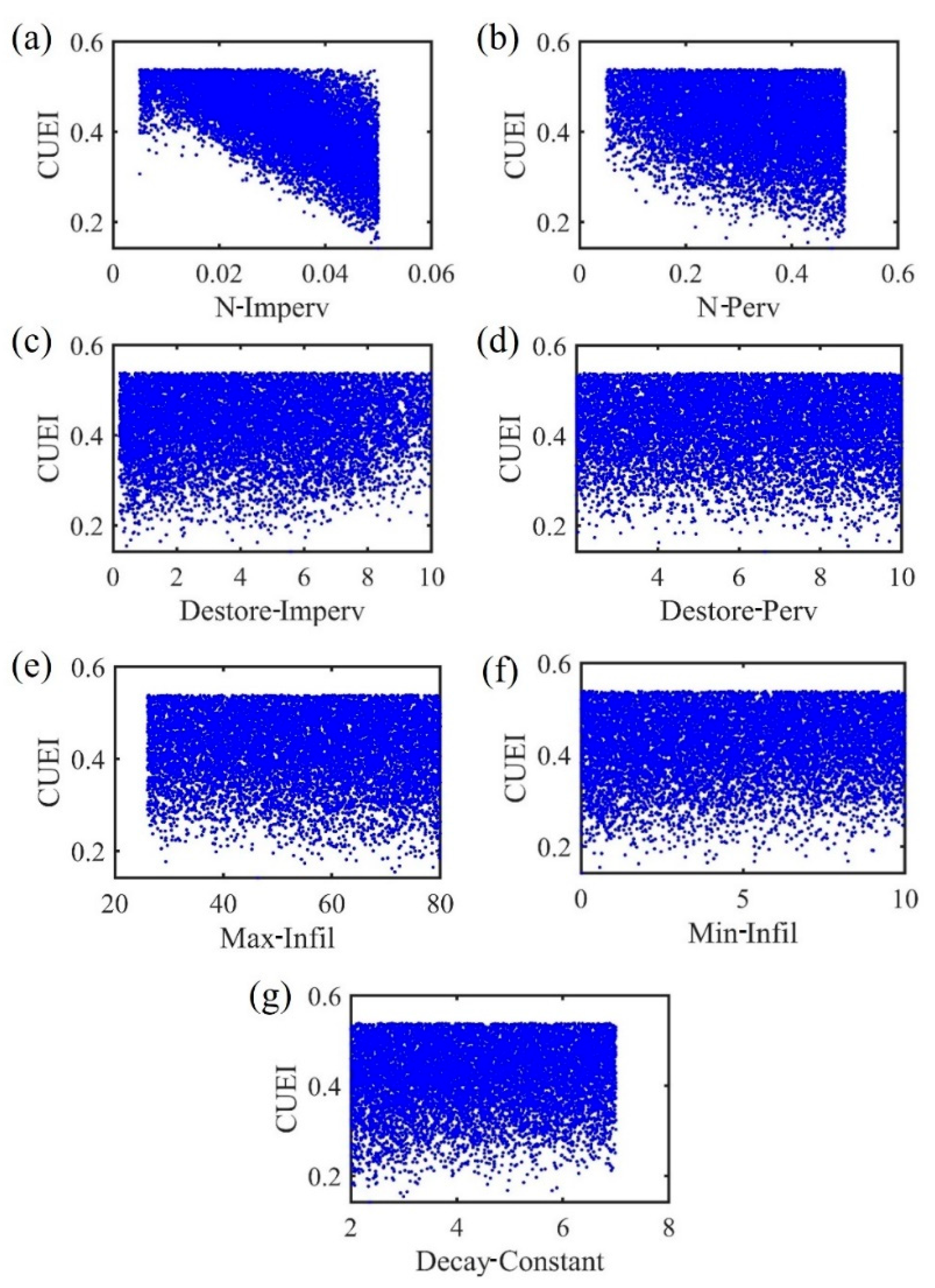
Based on the GLUE algorithm, Latin Hypercube Sampling (LHS) is used for random sampling of SWMM parameters, LID parameters, and different rainfall scenarios. A total of 10,000 parameter combinations that meet the criteria are selected using the uncertainty evaluation index, CUEI. The flow process at the drainage outlet is then simulated for each parameter combination. Figure 3 presents the uncertainty-distribution scatter plot for seven SWMM model parameters. The results indicate that the most significant uncertainty changes occur for the parameters N-Imperv, N-Perv, and Destore-Imperv. The likelihood variation in N-Imperv is the most pronounced, with a notable peak in the CUEI values occurring in the range of 0.4 to 0.5. As CUEI increases, the distribution of N-Perv and Destore-Imperv becomes more concentrated, while it becomes more dispersed when CUEI decreases. This suggests that these parameters are relatively sensitive. In contrast, the likelihood variations for the other parameters are minimal, indicating insensitivity to changes.

Table 1. Description of the parameters in SWMM.

Parameter	Meaning	Unit
N-Imperv	Roughness of impervious areas	/
N-Perv	Roughness of pervious areas	/
Destore-Imperv	Depth of depression storage on impervious areas	mm
Destore-Perv	Depth of depression storage on pervious areas	mm
Max-Infi	Maximum rate	mm/h
Min-Infi	Minimum rate	mm/h
Decay-Constant	Decay constant	h−1

provides the main parameters in SWMM.

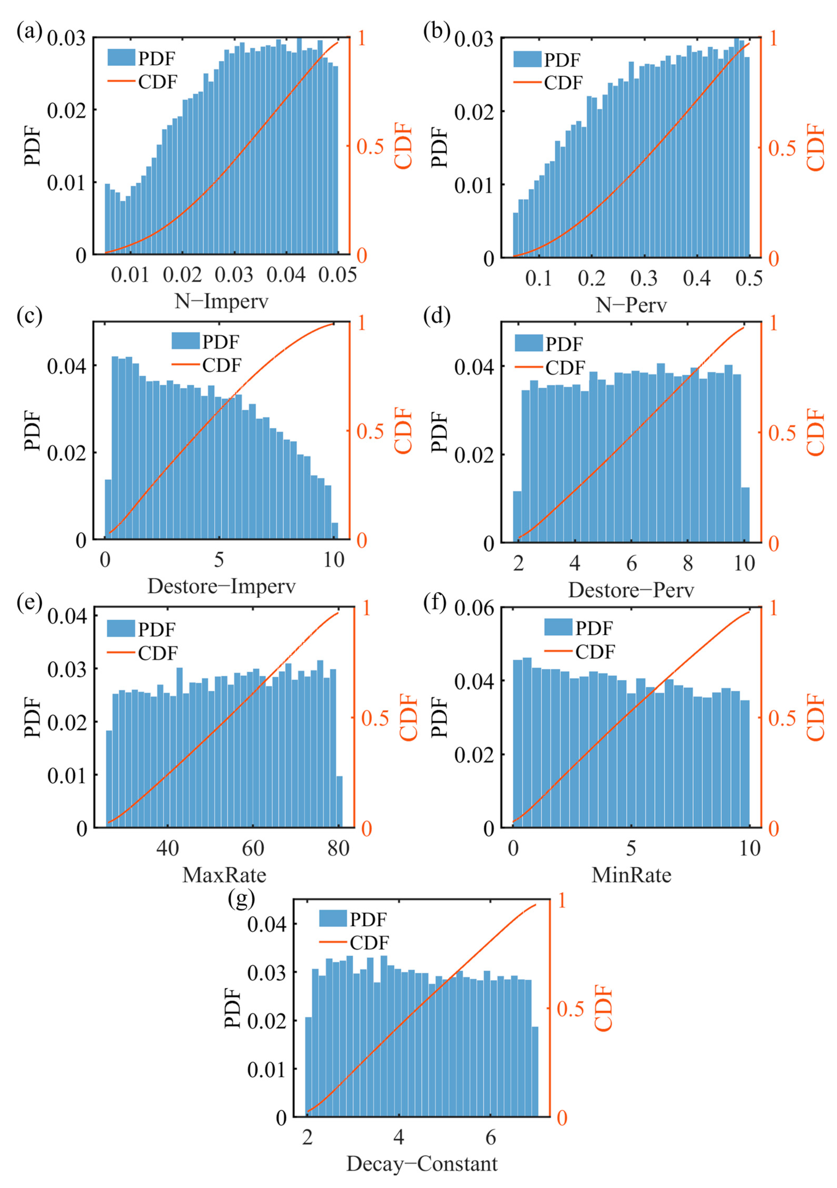
Figure 4 presents the changes in the probability density (PDF) and cumulative probability distribution (CDF) for seven parameters under random storm conditions. The posterior probability densities for the parameters N-Imperv, N-Perv, and Destore-Imperv exhibit non-uniform distributions, indicating their sensitivity, with N-Imperv showing the most significant variation. In contrast, the posterior distributions for the other four parameters remain largely consistent, with negligible changes in uncertainty, indicating their insensitivity. In urban areas with a high proportion of impervious surfaces, the infiltration capacity of hardened surfaces is poor, and parameters related to permeable surfaces and infiltration have a relatively weak effect on stormwater management. Additionally, under heavy rainfall conditions, the rapid surface runoff prevents rainwater from being discharged in time through the drainage system. When the drainage capacity of the network is saturated, overflow occurs, resulting in the minimal impact of parameter changes on model simulation outcomes.

To facilitate the evaluation of CUEI, this study will conduct a comprehensive analysis based on the calculation results and weights of each uncertainty indicator, according to the selection criteria shown in

Table 2. Uncertainty evaluation indicators and selection criteria.

Uncertainty Evaluation Indicators	Selection Criteria	Weight
NSE	>0.7	0.166
MSE	<10	0.168
RMSE	<2.5	0.165
N-S	≥0.6	0.172
REMR	<0.2	0.165
REMP	<0.2	0.164

.

Based on the GLUE method, multiple parameter combinations with significant correlations were selected to calculate the evaluation indicators of the symmetry of the uncertainty interval (

Table 3. Uncertainty interval evaluation indicators.

Indicators	Outfall O1	Outfall O2
Bw	2.35	0.69
D	2.07	0.51
CR	25.00	80.56
S	0.85	0.69

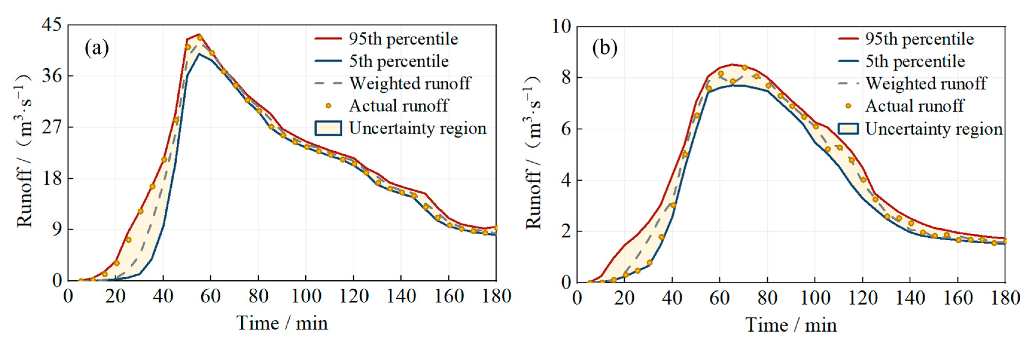
). Figure 5 presents the flow variation process for outfalls O1 and O2 under different parameter combinations and shows the outflow range for the drainage outlets within the 95% confidence interval of the parameters. For outlet O1, B_w is 2.35, D is 2.07, CR is 25.00, and S is 0.85. In contrast, for outlet O2, B_w is 0.69, D is 0.51, CR is 80.56, and S is 0.69. It can be observed that the B_w, D, and S values for O1 are higher than those for O2, indicating greater uncertainty in the model for O1. Meanwhile, CR for O2 is significantly higher than that of O1, suggesting that O2 exhibits a broader range of variability, reflecting stronger uncertainty influences. Overall, the parameters for O2 show greater volatility, whereas O1 remains relatively stable.

4.2. Analysis of Control Effect Based on Posterior Distribution (PODM)

4.2.1. Edge Distribution Fitting of Governance Effect Index Based on PODM

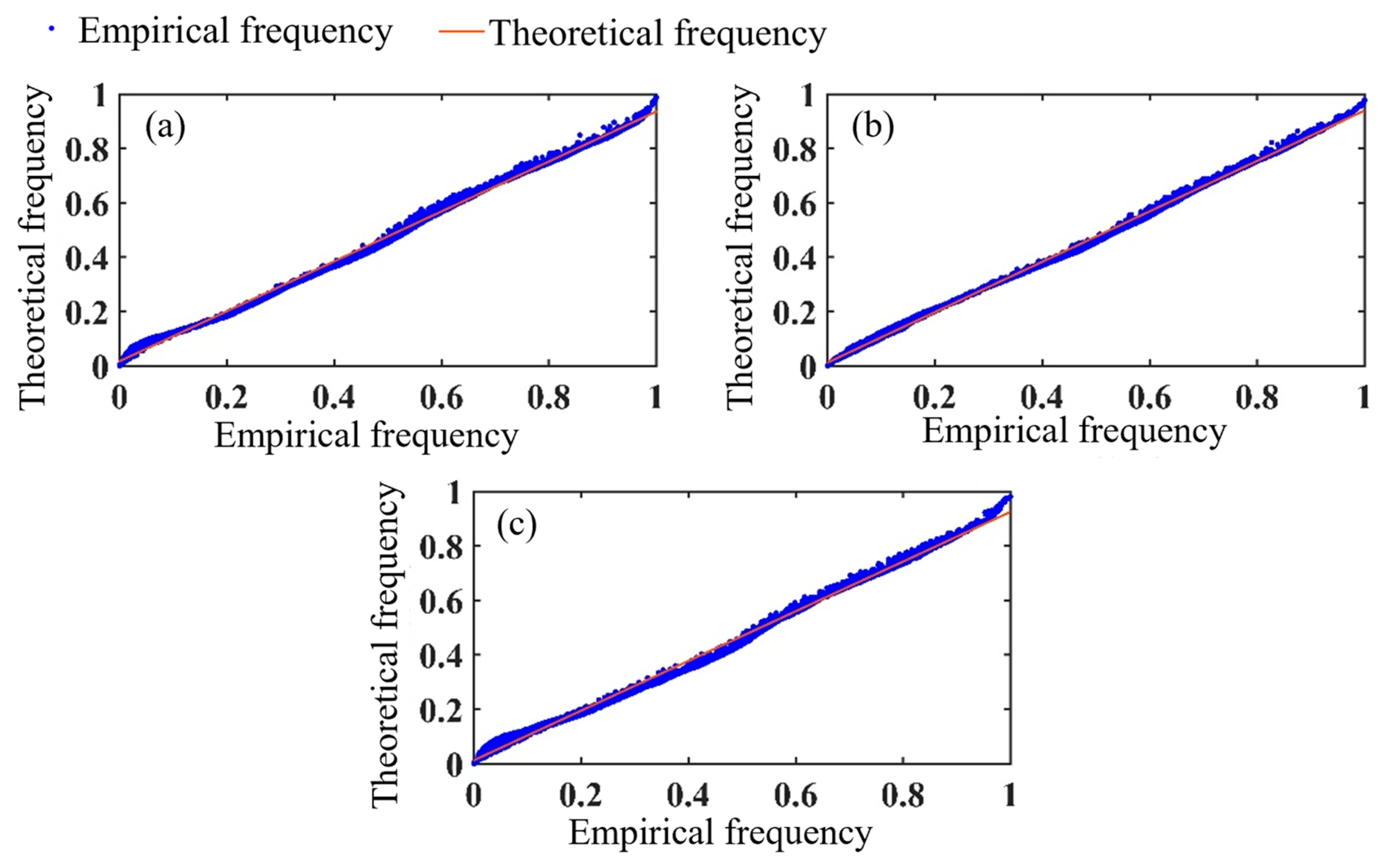
Based on the GLUE uncertainty analysis results, the posterior distribution of SWMM parameters is used for marginal fitting to achieve a joint analysis of the control-effect evaluation indicators. The evaluation indicators, including surface-runoff reduction rate (S_R), peak-flow reduction rate at outfall O2 (S₂₁₀), and peak-flow reduction rate at outfall O4 (S₄₅), are jointly analyzed. The frequency values of flood-control effectiveness indicators are calculated using the cumulative distribution function, and empirical and theoretical frequency distributions are plotted (Figure 6). Theoretical and empirical frequencies calculated using the Copula function both distribute closely along the 45° line, indicating that the fitting performance using kernel-density non-parametric test methods is quite good.

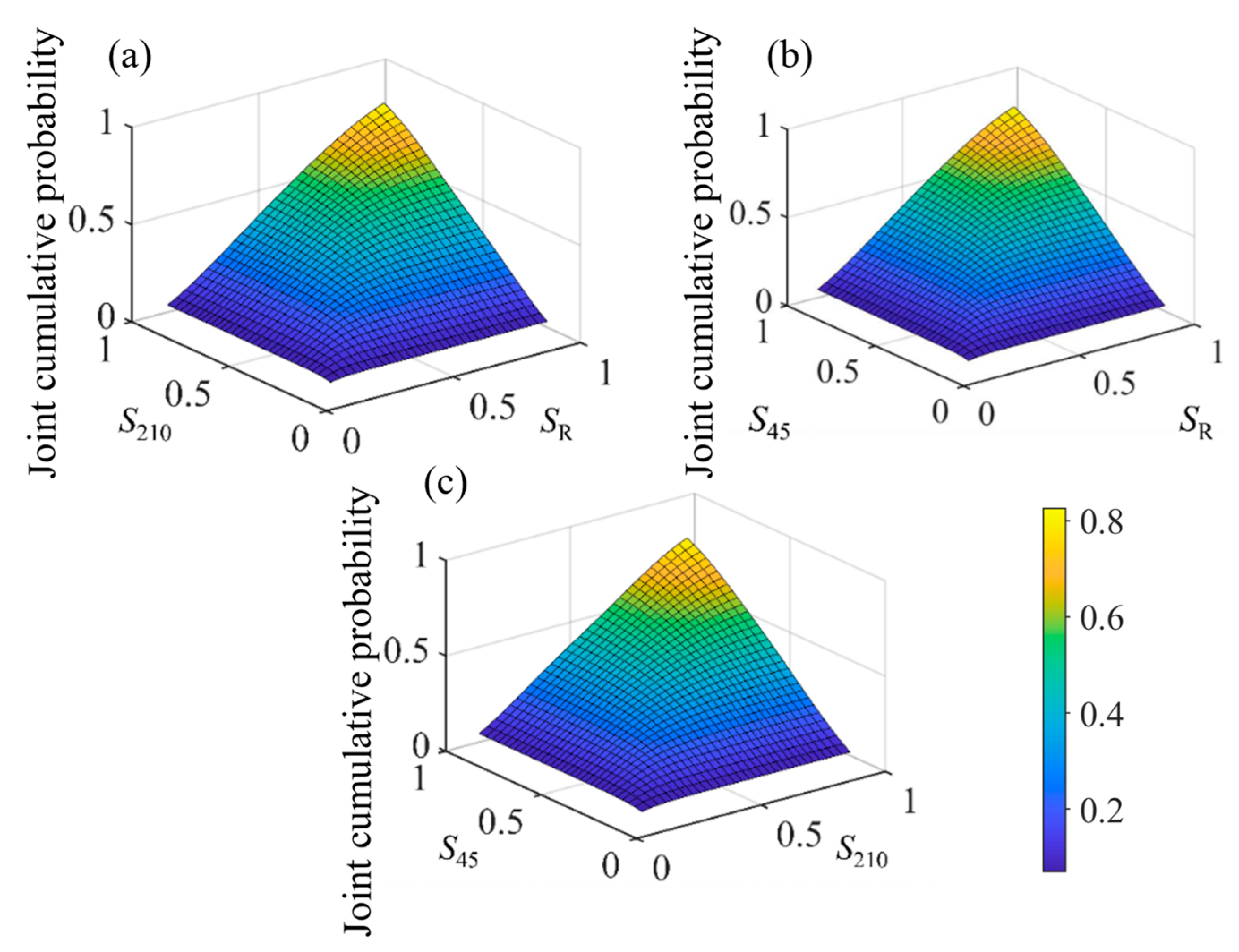
Figure 7 presents the joint probability distributions. As S_R and S₂₁₀ increase, the overall control effect continues to improve, showing a trend of increasing initially and then decreasing.

4.2.2. Joint Distribution of Surface-Runoff Reduction Rate and Peak-Flow Reduction Rate Based on PODM

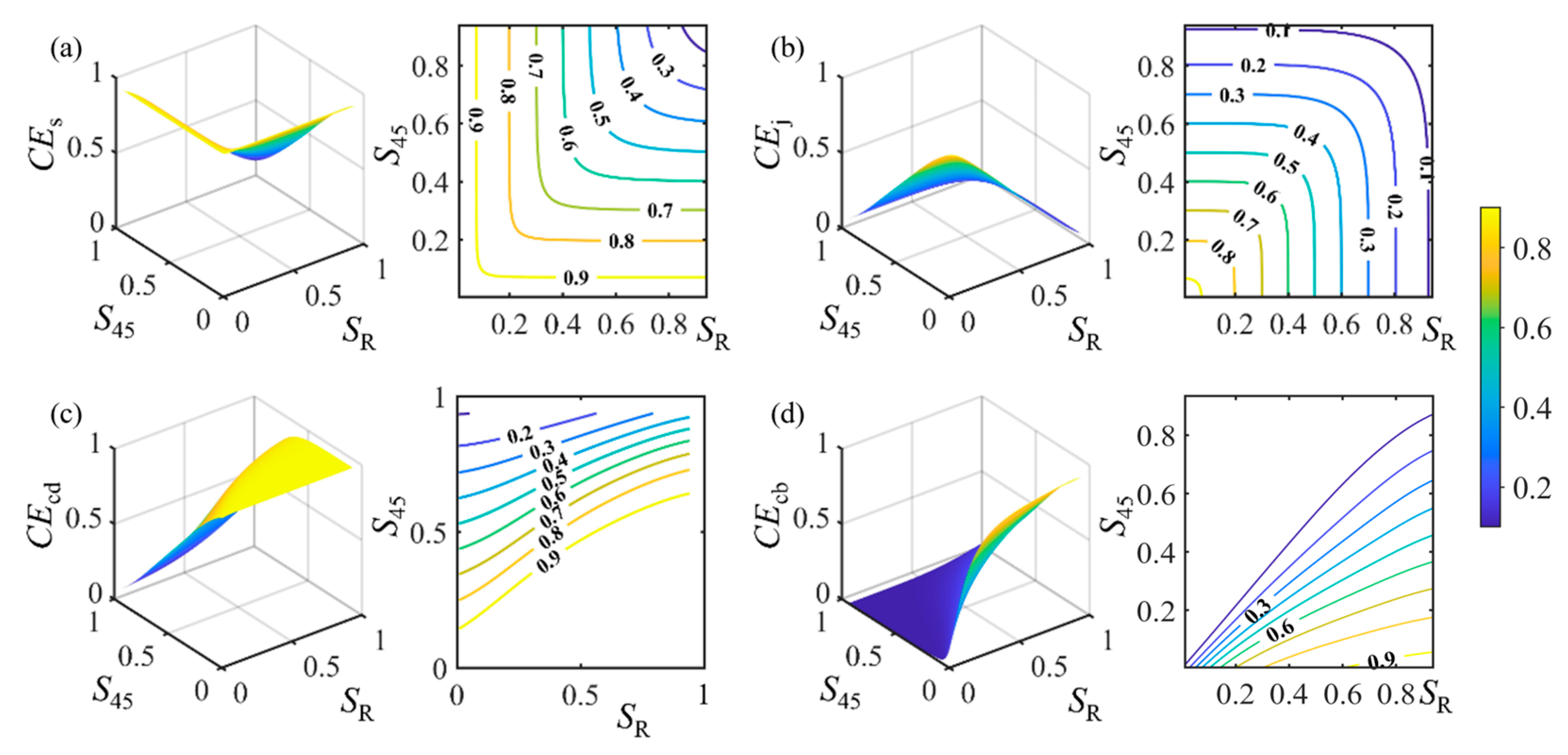
The denser the contour lines, the smaller the fluctuations of this variable; conversely, it indicates greater parameter variability, and the trend line of the joint control-effect distribution will be biased toward the side with denser contour lines. Figure 8 presents the control effects of S_R and S₂₁₀. CE_s decreases as S_R and S₂₁₀ increase. When S_R and S₂₁₀ are 0.84% and 1.37%, respectively, CE_s reaches 94.81%. However, when S_R and S₂₁₀ reach 94.15% and 92.73%, the control efficiency drops to 14.76%. When S_R reaches 75% and S₂₁₀ is below 7.56%, the joint control effect can exceed 90%. However, when S₂₁₀ exceeds 82.73%, the control effect falls below 30%. When S_R and S₂₁₀ are 1.00% and 1.47%, CE_j reaches its maximum value of 93.06%, but subsequently, CE_j decreases as S_R and S₂₁₀ increase. When S_R reaches 75%, the value of CE_j fluctuates between 0% and 24.99% with changes in S₂₁₀. When S_R remains constant, CE_cd decreases as S₂₁₀ increases, and the rate of decrease becomes slower as S_R increases. When S₂₁₀ is below 30%, CE_cd remains relatively stable with changes in S_R. However, when S₂₁₀ exceeds 30%, CE_cd increases significantly with S_R, although the rate of increase slows as S₂₁₀ increases. When S₂₁₀ is fixed, CE_cb increases gradually as S_R increases. The rate of increase first rises and then decreases with higher values of S₂₁₀. When S₂₁₀ is 30.12%, CE_cb increases from 13.49% at S_R = 34.33% to 59.32% at S_R = 75.00%. When S_R remains constant, CE_cb gradually decreases as S₂₁₀ increases, and the rate of change diminishes as S_R increases. When S_R is 75.01%, CE_cb reaches its maximum value of 91.93% at S₂₁₀ = 1.37%, and falls below 10% when S_R exceeds 76.74%.

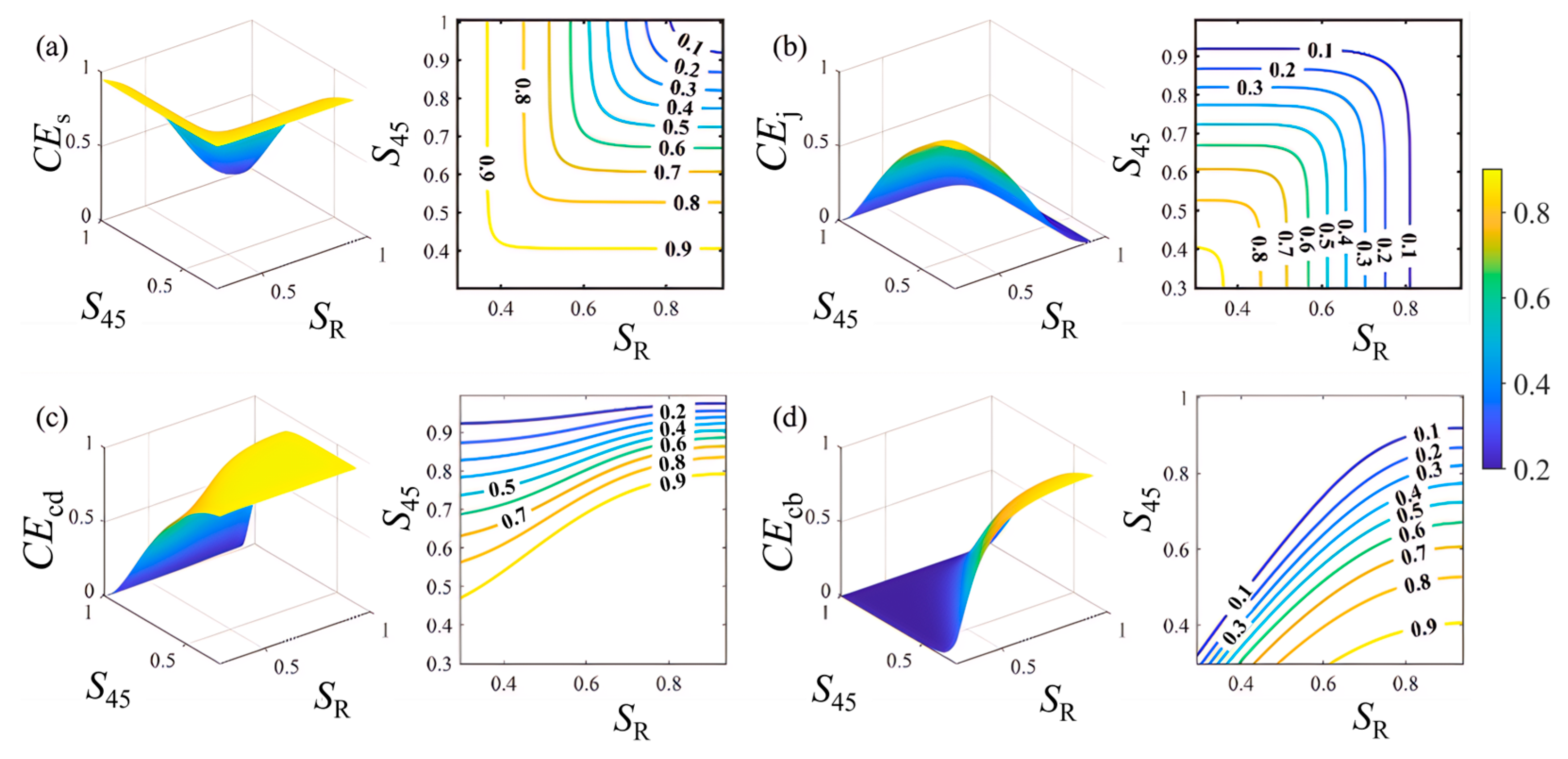
Figure 9 presents the control effects of S_R and S₄₅. CE_s decreases as S_R and S₄₅ increase. When S_R and S₄₅ are 0.90% and 0.37%, respectively, CE_s reaches its maximum value of 94.79%. However, when S_R and S₄₅ exceed 92.65% and 71.77%, CE_s drops below 30%. When S_R and S₄₅ are 0.92% and 0.56%, CE_j reaches its maximum value of 93.08%, but subsequently, CE_j decreases as S_R and S₄₅ increase. When S_R remains constant, CE_cd decreases as S₄₅ increases, and the rate of decrease becomes slower as S_R increases. When S₄₅ is below 30%, CE_cd remains relatively stable with changes in S_R. However, when S₄₅ exceeds 30%, CE_cd increases significantly with S_R, although the rate of increase slows as S₄₅ increases. When S₄₅ is fixed, CE_cb increases gradually as S_R increases. The rate of increase first rises and then decreases with higher values of S₄₅. When S₄₅ is 70.06%, CE_cb reaches a maximum value of 24.65% at S_R = 93.97%. When S_R remains constant, CE_cb decreases as S₄₅ increases. When S_R is relatively small, CE_cb decreases significantly as S₄₅ increases. When S_R is 75.08%, CE_cb remains above 80% when S₄₅ exceeds 13.61%, respectively. However, when S₄₅ exceeds 54.16%, CE_cb drops below 30%.

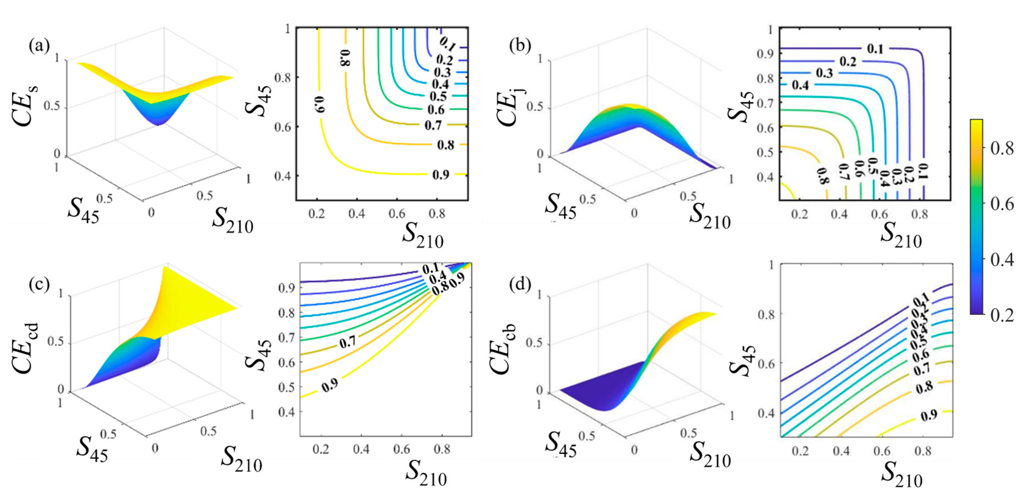
4.2.3. Joint Distribution of Peak-Flow Reduction Rate Based on PODM

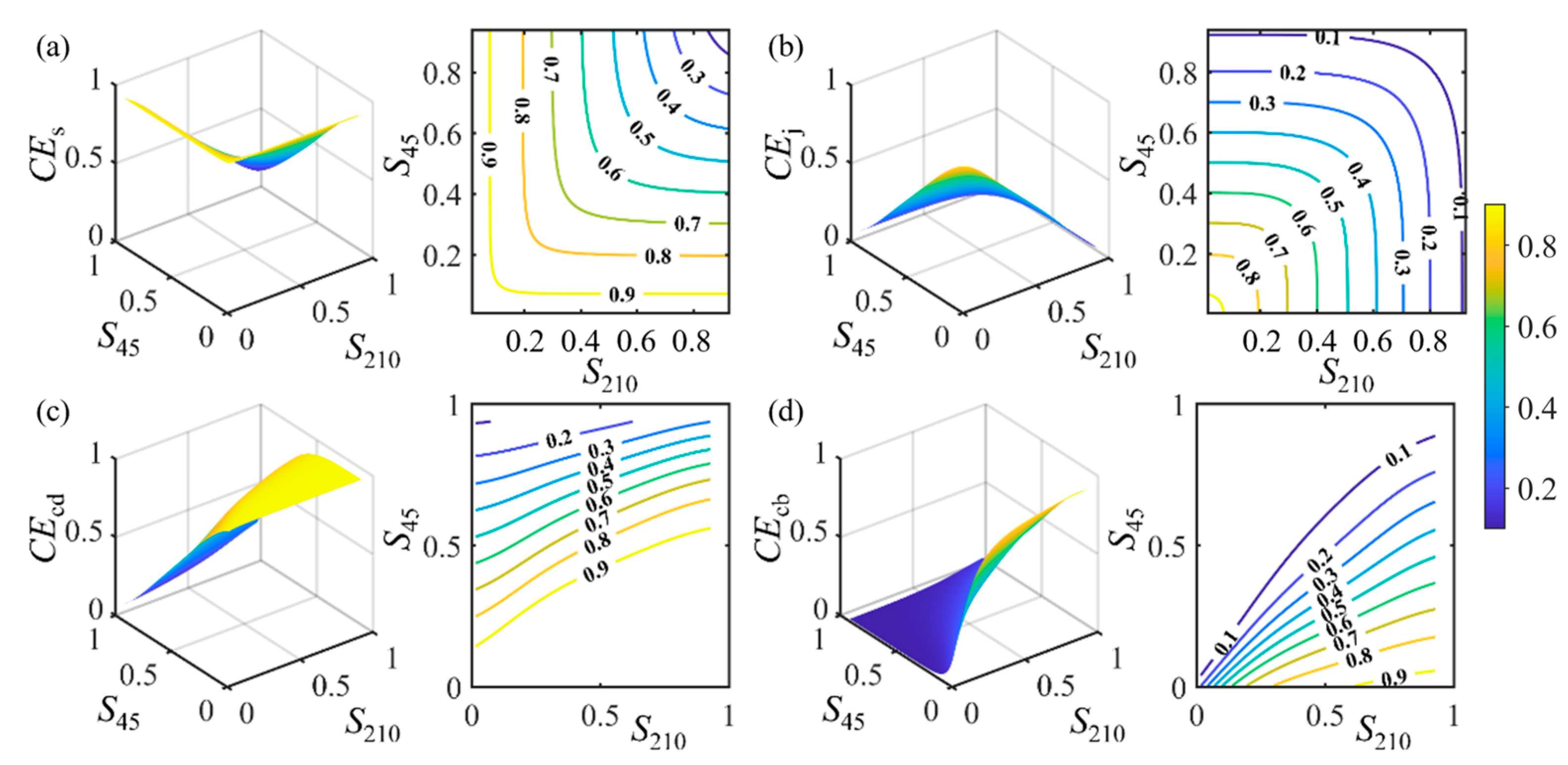
Figure 10 presents the control effects of S₂₁₀ and S₄₅. CE_s decreases as S₂₁₀ and S₄₅ increase. CE_s decreases as S₂₁₀ and S₄₅ increase, reaching a maximum of 95.04% when S₂₁₀ is 1.31% and S₄₅ is 0.86%. CE_s shows larger variation with smaller S₂₁₀ as S₄₅ increases. Similarly, CE_j reaches a maximum of 92.76% when S₂₁₀ is 1.50% and S₄₅ is 0.42%, then decreases as both increase. When S₂₁₀ exceeds 70.49%, CE_j remains below 30% regardless of S₄₅. When S₂₁₀ is fixed, CE_cd decreases as S₄₅ increases, with a more significant decrease at larger S₂₁₀ values. When S₄₅ is small, CE_cd increases slightly with S₂₁₀, but the change becomes more significant at larger S₄₅, especially with high S₂₁₀. When S₂₁₀ is 60.08%, CE_cd stays above 80% if S₄₅ is below 55.83%, and below 30.01% if S₄₅ exceeds 86.87%. When S₂₁₀ is fixed, CE_cb decreases as S₄₅ increases. The change is more significant at smaller S₂₁₀ and uniform at larger values. When S₄₅ is small, CE_cb changes more with smaller S₂₁₀, but remains stable at larger S₂₁₀. When S₂₁₀ is 60.62%, CE_cb stays above 80% if S₄₅ is below 9.80%, and below 30.20% if S₄₅ exceeds 45.58%.

4.3. Analysis of Control Effect Based on Prior Distribution (PRDM)

4.3.1. Edge Distribution Fitting of Governance Effect Index Based on PRDM

Using a non-parametric kernel-density analysis method, the frequency values of the flood-control effectiveness indicators are calculated based on the cumulative distribution function, resulting in empirical and theoretical frequency distributions (Figure 11). The theoretical and empirical frequencies calculated using the Copula function are both distributed near the 45° line, indicating a good fitting performance.

Based on the optimized Gumbel Copula function, the joint probability distribution of the variables is constructed (Figure 12). As S_R and S₂₁₀ increase, the overall control effect continues to improve, exhibiting a trend of increasing initially and then decreasing.

4.3.2. Joint Distribution of Surface-Runoff Reduction Rate and Peak-Flow Reduction Rate Based on PRDM

Figure 13 presents the control effects of S_R and S₂₁₀. CE_s decreases as S_R and S₂₁₀ increase. When S_R and S₂₁₀ are 29.32% and 10.00%, respectively, CE_s reaches its maximum value of 97.41%. When S_R reaches 75%, and S₂₁₀ is less than 21.1%, the joint control effect can exceed 90%. However, when S₂₁₀ exceeds 69.78%, the joint control effect falls below 30%. When S_R and S₂₁₀ are 29.37% and 10.51%, respectively, CE_j reaches its maximum value of 92.28%, after which CE_j gradually decreases as S_R and S₂₁₀ increase. When S_R remains constant, CE_cd decreases as S₂₁₀ increases. The larger S_R becomes, the more gradual the decrease in CE_cd as S₂₁₀ increases. When S₂₁₀ is below 30%, CE_cd remains relatively stable with changes in S_R. However, when S₂₁₀ exceeds 30%, CE_cd increases significantly with S_R, although the rate of increase slows as S₂₁₀ increases. When S₂₁₀ is fixed, CE_cb increases gradually as S_R increases. The rate of increase first rises and then decreases with higher values of S₂₁₀. When S₂₁₀ is 30.12%, CE_cb increases from 20.12% at S_R = 34.48% to 79.66% at S_R = 75.01%. When S_R remains constant, CE_cb decreases as S₂₁₀ increases. The rate of decrease becomes slower as S_R increases. When S_R is 75.01%, CE_cb increases from 9.92% at S₂₁₀ = 9.92% to a maximum value of 93.56% at S₂₁₀ = 44.45%.

Figure 14 presents the control effects of S_R and S₄₅. CE_s decreases as S_R and S₄₅ increase. When S_R and S₄₅ are 29.47% and 30.08%, respectively, CE_s reaches its maximum value of 95.68%. However, when S_R and S₄₅ exceed 71.20% and 92.61%, CE_s falls below 30%. When S_R and S₄₅ are 30.01% and 29.79%, respectively, CE_j reaches its maximum value of 93.99%, after which CE_j decreases gradually as S_R and S₄₅ increase. When S_R exceeds 70.33% and S₄₅ exceeds 56.88%, CE_j remains below 30%. When S_R remains constant, CE_cd decreases as S₄₅ increases, and the rate of decrease becomes slower as S_R increases. Conversely, when S₄₅ is below 70%, CE_cd decreases uniformly with S_R. However, when S₄₅ exceeds 70%, CE_cd shows a decreasing trend that first slows and then accelerates as S_R increases. When S_R reaches 75%, CE_cd remains below 20.12%, and when S₄₅ exceeds 88.30%, CE_cd drops below 10%. When S₄₅ is fixed, CE_cb increases gradually as S_R increases. The rate of increase first rises and then decreases as S₄₅ increases. When S₄₅ is 70.03%, CE_cb increases from 74% at S_R = 50.12% to 97.69% at S_R = 80.09%, and reaches its maximum value of 98.29% at S_R = 93.80%. When S_R remains constant, CE_cb decreases as S₄₅ increases, and the rate of change first decreases and then increases as S_R increases.

4.3.3. Joint Distribution of Peak-Flow Reduction Rate Based on PRDM

Figure 15 presents the control effects of S₂₁₀ and S₄₅. CE_s decreases as S₂₁₀ and S₄₅ increase. When S₂₁₀ and S₄₅ are 9.73% and 29.87%, respectively, CE_s reaches its maximum value of 97.42%. However, CE_s remains above 40% as S₄₅ continues to increase. Compared to situations with larger values of S₂₁₀, when S₂₁₀ is smaller, CE_s exhibits a larger variation as S₄₅ increases, and S₄₅ follows a similar pattern of change. When S₂₁₀ and S₄₅ are 9.77% and 30.18%, respectively, CE_j reaches its maximum value of 92.41%, after which CE_j decreases gradually as S₂₁₀ and S₄₅ increase. When S₂₁₀ exceeds 28.81%, CE_j remains below 30% with changes in S₄₅. When S₂₁₀ remains constant, CE_cd decreases as S₄₅ increases. The decrease is uniform when S₂₁₀ is small, but more significant when S₂₁₀ is large. When S₄₅ is constant, CE_cd increases with S₂₁₀, with a more pronounced change at higher S₄₅ values. When S₂₁₀ is constant, CE_cb decreases as S₄₅ increases. The change is more significant at smaller S₂₁₀ and uniform at larger S₂₁₀. When S₄₅ is small, CE_cb changes more significantly with smaller S₂₁₀; when S₄₅ is large, CE_cb stays stable as S₂₁₀ increases. When S₂₁₀ is 60.04%, CE_cb stays above 80% if S₄₅ is below 42.13%, and below 30% if S₄₅ exceeds 67.43%.

4.4. Comparison and Analysis of PODM and PRDM Management Effectiveness

Based on the LID treatment effects obtained through prior and posterior analysis, the trends of change under different conditions are similar. In the evaluation of treatment effects, when indicators E₁ and E₂ remain unchanged, CE_s varies with the increase in E₂, showing a smaller variation. However, when both E₂ and E₁ change, the variation in CE_j increases with the increase in E₂, and the volatility of the treatment effect becomes larger. Furthermore, when E₂ changes over a larger time scale, the treatment effect shows more significant changes, while CE_cd decreases with the increase in E₂, exhibiting smaller fluctuations in the treatment effect. Lastly, when E₂ remains unchanged, CE_cb shows a trend of changing with the increase in E₁, and the volatility of the treatment effect is larger.

4.5. Limitations and Application Value

This study evaluates the uncertainty of the SWMM model using the GLUE method and deeply analyzes the rainwater and flood-control benefits of LID through the Copula method, providing a comprehensive analysis framework. By performing parameter sampling under both prior and posterior distributions and combining the Copula method to assess LID’s rainwater and flood-control benefits, the study effectively captures the impact of uncertainty on the results. This approach not only considers the uncertainty of model parameters, avoiding the limitations of LID benefit analysis under a single condition, but also simulates LID performance under different scenarios, providing support for understanding the overall rainwater and flood-control benefits of LID under various conditions. Based on this framework, we can more effectively select and adjust LID measures to improve the adaptability and accuracy of urban stormwater management.

This study still has certain limitations. Firstly, LID parameters rely on empirical data and are often difficult to determine precisely, so the results of the uncertainty analysis may be influenced by parameter assignment and model assumptions. Additionally, although sampling from the posterior distribution is more realistic than using a uniform distribution, the heteroscedasticity of parameters may still affect the results, especially in applications across different regions and rainfall patterns. Therefore, urban managers need to carefully adjust LID designs and parameter settings based on local experience and actual conditions to ensure optimized rainwater and flood-control effects. Thus, this research aids in evaluating the effectiveness of various LID implementation strategies, promoting environmental protection, water conservation, and climate adaptation goals in alignment with sustainable development objectives.

5. Conclusions

We have developed an analytical framework for evaluating urban pluvial-flood-control uncertainty, with the following main conclusions:

(1) The GLUE method can identify the sensitive parameters of the model and calculate the uncertainty in regional drainage processes. The highly sensitive parameters of SWMM are the Manning’s coefficient for impervious surfaces, the Manning’s coefficient for pervious surfaces, and the impervious surface-depression storage. The sensitivity differences in the other parameters are relatively small under different rainfall scenarios. The GLUE method can select multiple sets of equivalent simulation-parameter combinations and characterize the parameter interactions and heterogeneous parameter equivalence present in the hydrological model.

(2) Based on the analysis, the model uncertainty for outlet O1 is higher than for O2, as indicated by the higher values of B (2.35), D (2.07), and S (0.85) for O1. This suggests that O1 has more stability in its uncertainty. In contrast, outlet O2 shows lower values of B (0.69), D (0.51), and S (0.69), but a significantly higher CR (80.56), indicating a wider range of uncertainty and greater variability. In summary, O2 is more volatile, while O1 remains more stable.

(3) A comparison of the posterior and prior joint distributions of uncertainty based on the GLUE method reveals that for different governance performance metrics, the joint governance effect, synergistic governance effect, conditional governance effect, and combined governance effect exhibit consistent patterns of variation, with differences in their ranges.

The framework provides valuable assistance in analyzing uncertainty in urban pluvial-flood control and urban sustainable development.