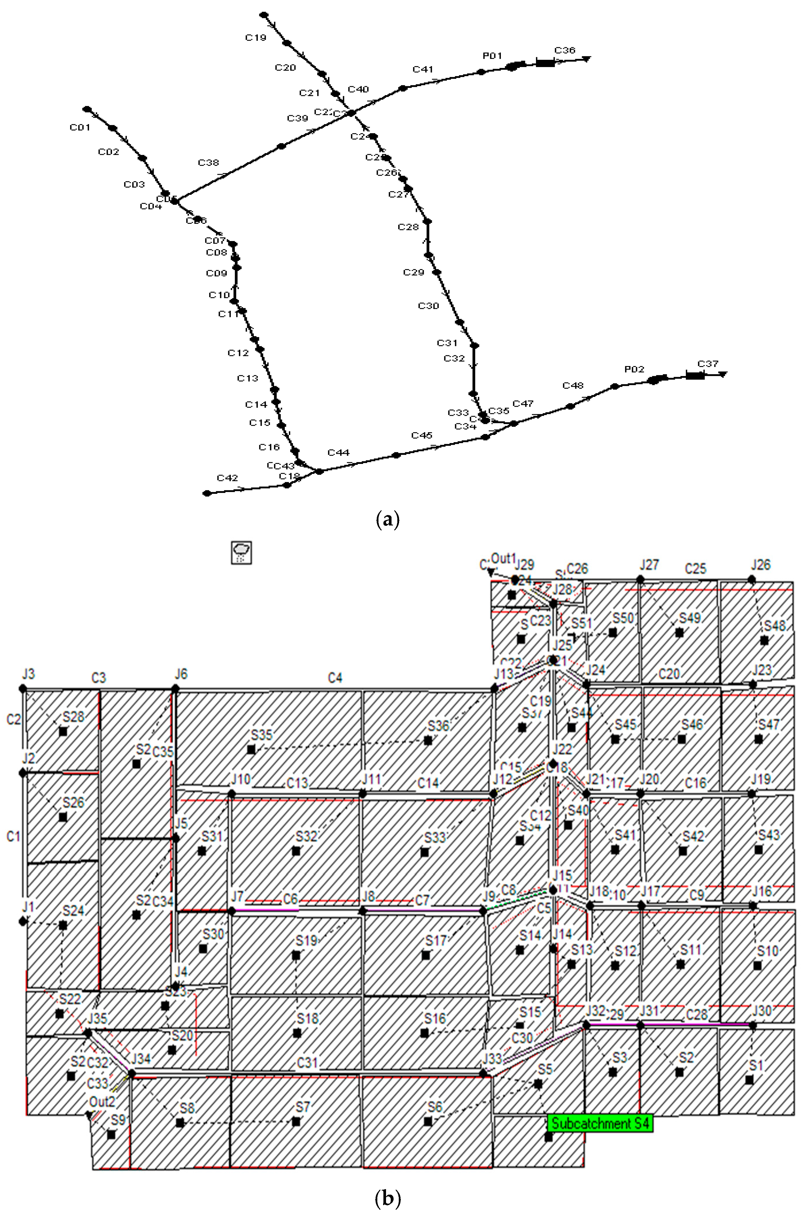
Figure 1.
(a) Pipe network layout diagram; (b) SWMM diagram for the study area. The black lines with nodes (labelled J1, J2, etc.) and connections represent the structural framework of the system. Red indicates specific flow paths or important connections within the system. Purple lines indicate different types of flow paths or special features in the system. The green text ‘Subcatchment S4’ clearly identifies specific subcatchments within the larger system.
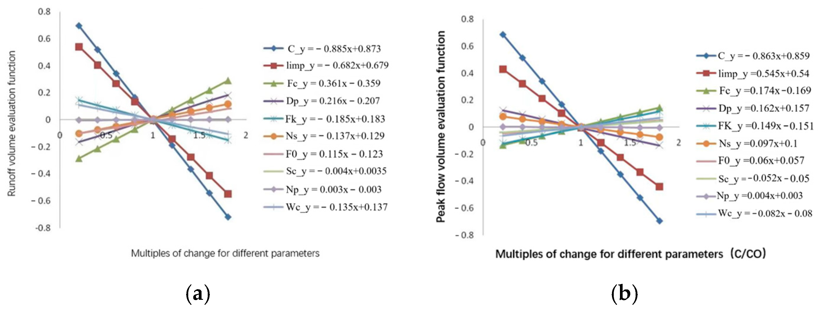
Figure 2.
The results of the parameter sensitivity analyses. (a) The relative error in runoff volume, and (b) the relative error in runoff peak discharge. The number of parameter variations is plotted on the x-axis, while the corresponding equilibrium function values are plotted on the y-axis. A linear regression curve was generated to analyze the data.
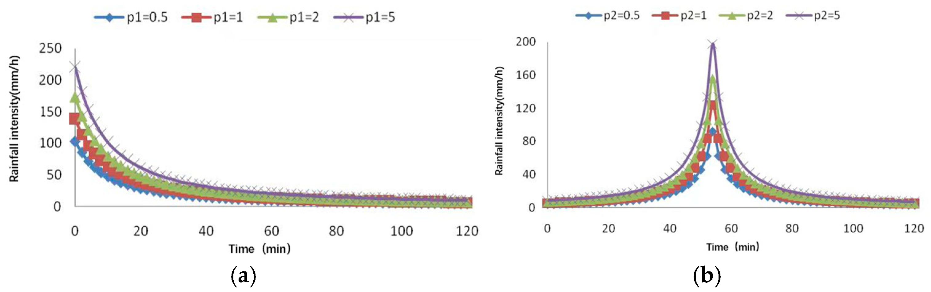
Figure 3.
Chicago synthetic rainfall process lines for different rainfall intensities: (a) rainfall process line for rainfall intensity r = 0, and (b) rainfall process line for rainfall intensity r = 0.45.
Figure 3.
Chicago synthetic rainfall process lines for different rainfall intensities: (a) rainfall process line for rainfall intensity r = 0, and (b) rainfall process line for rainfall intensity r = 0.45.
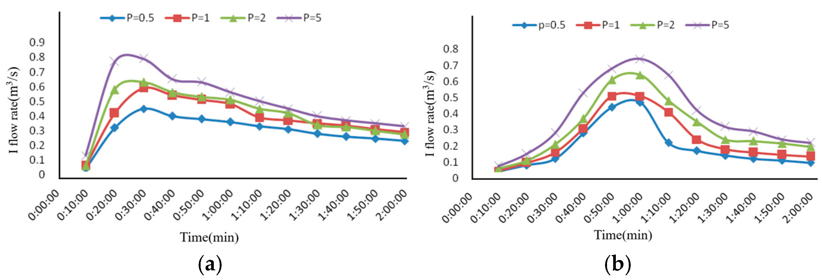
Figure 4.
Flow process line at the outlet under different rainfall intensities: (a) flow process line at the outlet for rainfall intensity r = 0, and (b) flow process line at the outlet for rainfall intensity r = 0.45.
Figure 4.
Flow process line at the outlet under different rainfall intensities: (a) flow process line at the outlet for rainfall intensity r = 0, and (b) flow process line at the outlet for rainfall intensity r = 0.45.
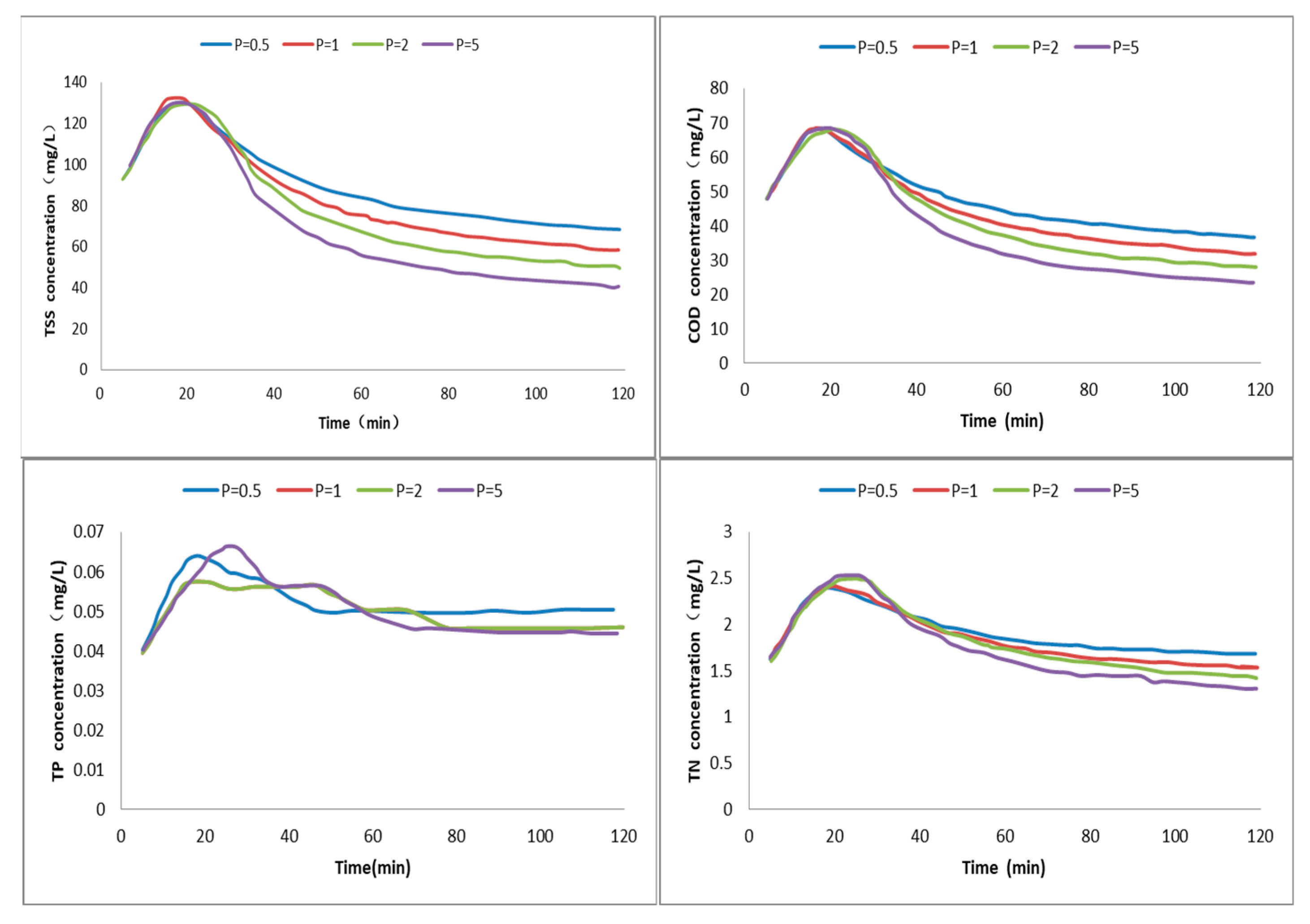
Figure 5.
The pattern of pollutant concentration changes at the outlet of the pipe network for rainfall intensity r = 0.
Figure 5.
The pattern of pollutant concentration changes at the outlet of the pipe network for rainfall intensity r = 0.
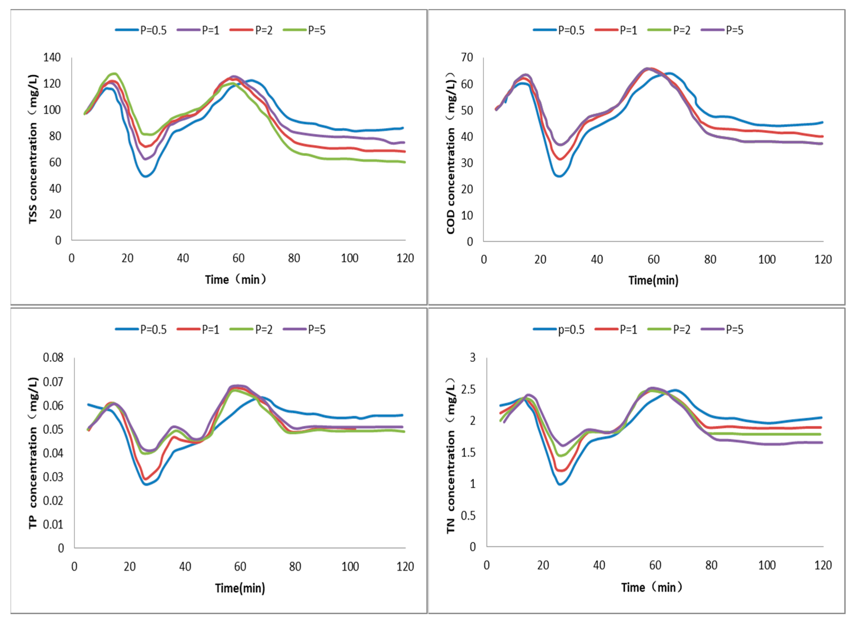
Figure 6.
The pattern of pollutant concentration changes at the outlet of the pipe network for rainfall intensity r = 0.45.
Figure 6.
The pattern of pollutant concentration changes at the outlet of the pipe network for rainfall intensity r = 0.45.
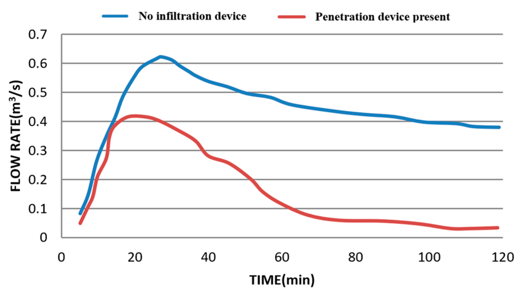
Figure 7.
Changes in outlet flow before and after implementing permeable pavements and ditches. The red line represents the rainfall–runoff curve for the Chicago rainfall pattern with permeable pavements, while the blue line represents the rainfall–runoff curve for the case without a permeable pavement.
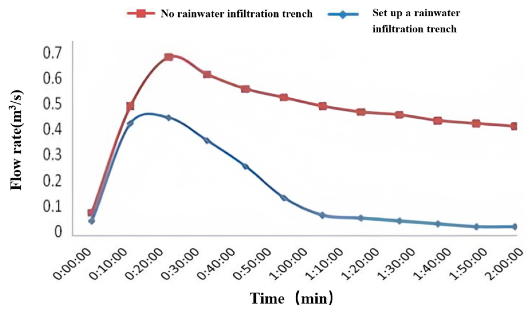
Figure 8.
Comparison of the flow process lines of the egress nodes before and after implementing the infiltration ditch. The red line represents the runoff without ditches, while the blue line represents the runoff with ditches.
Figure 8.
Comparison of the flow process lines of the egress nodes before and after implementing the infiltration ditch. The red line represents the runoff without ditches, while the blue line represents the runoff with ditches.
Figure 9.
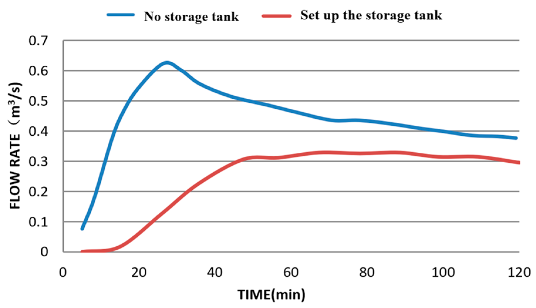
Changes in outlet flow before and after implementing the storage tank. The red line represents the runoff process with regulation and storage, while the blue line represents the runoff without these measures.
Figure 9.
Changes in outlet flow before and after implementing the storage tank. The red line represents the runoff process with regulation and storage, while the blue line represents the runoff without these measures.
Figure 10.
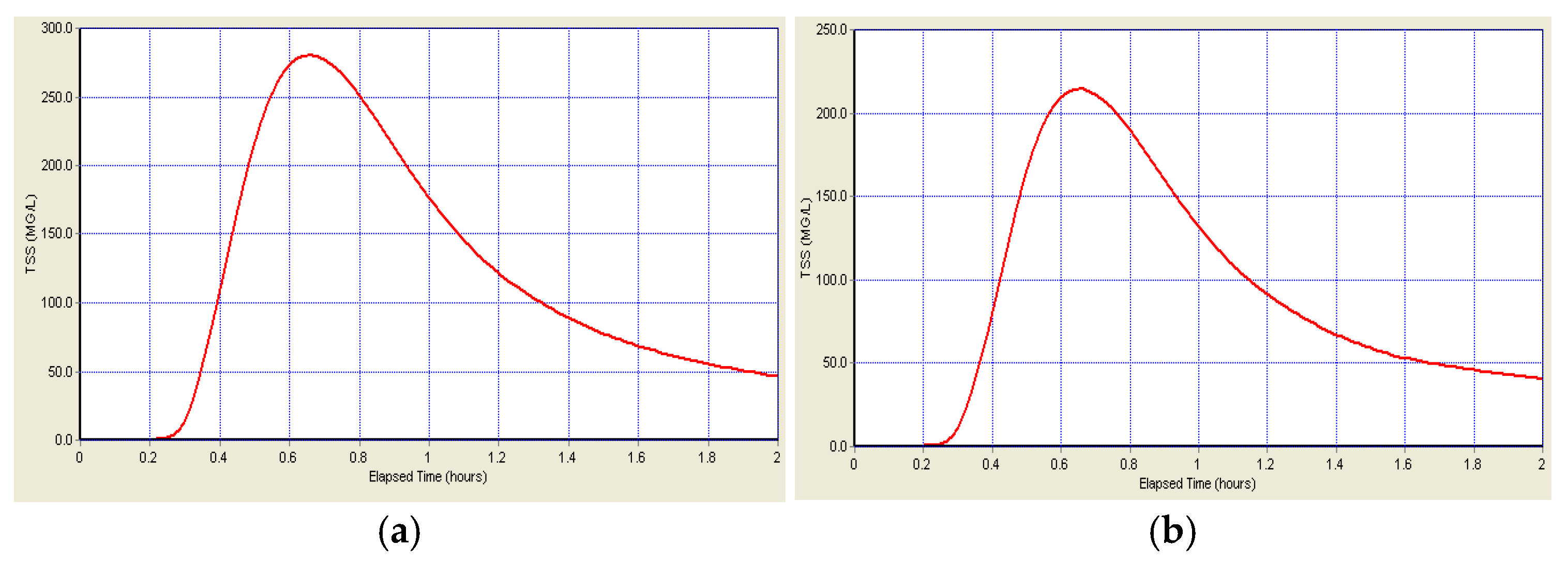
The TSS concentration before and after adding the storage tank: (a) the maximum TSS concentration at the outlet node before adding the storage tank is 280 mg/L, and (b) the maximum TSS concentration at the outlet node after adding the storage tank is 215 mg/L.
Figure 10.
The TSS concentration before and after adding the storage tank: (a) the maximum TSS concentration at the outlet node before adding the storage tank is 280 mg/L, and (b) the maximum TSS concentration at the outlet node after adding the storage tank is 215 mg/L.
Figure 11.
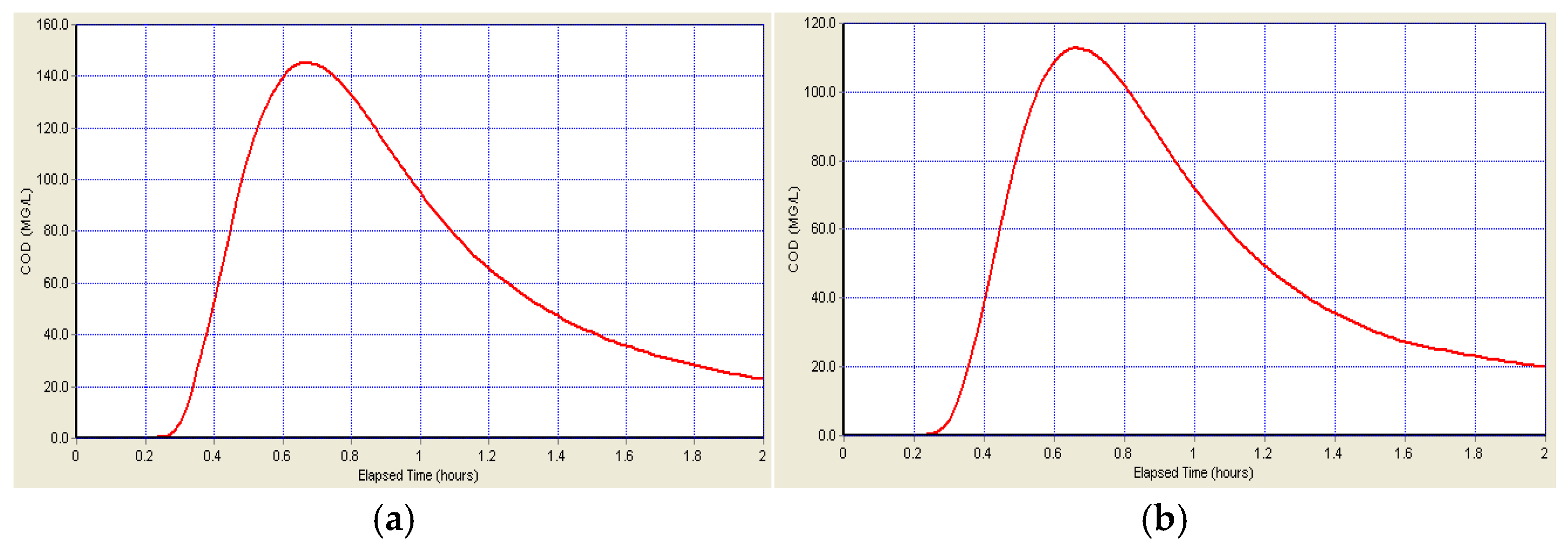
The COD concentration before and after adding the storage tank: (a) the COD concentration at the outlet node before adding the storage tank is 155 mg/L, and (b) the COD concentration at the outlet node after adding the storage tank is 110 mg/L.
Figure 11.
The COD concentration before and after adding the storage tank: (a) the COD concentration at the outlet node before adding the storage tank is 155 mg/L, and (b) the COD concentration at the outlet node after adding the storage tank is 110 mg/L.
Figure 12.
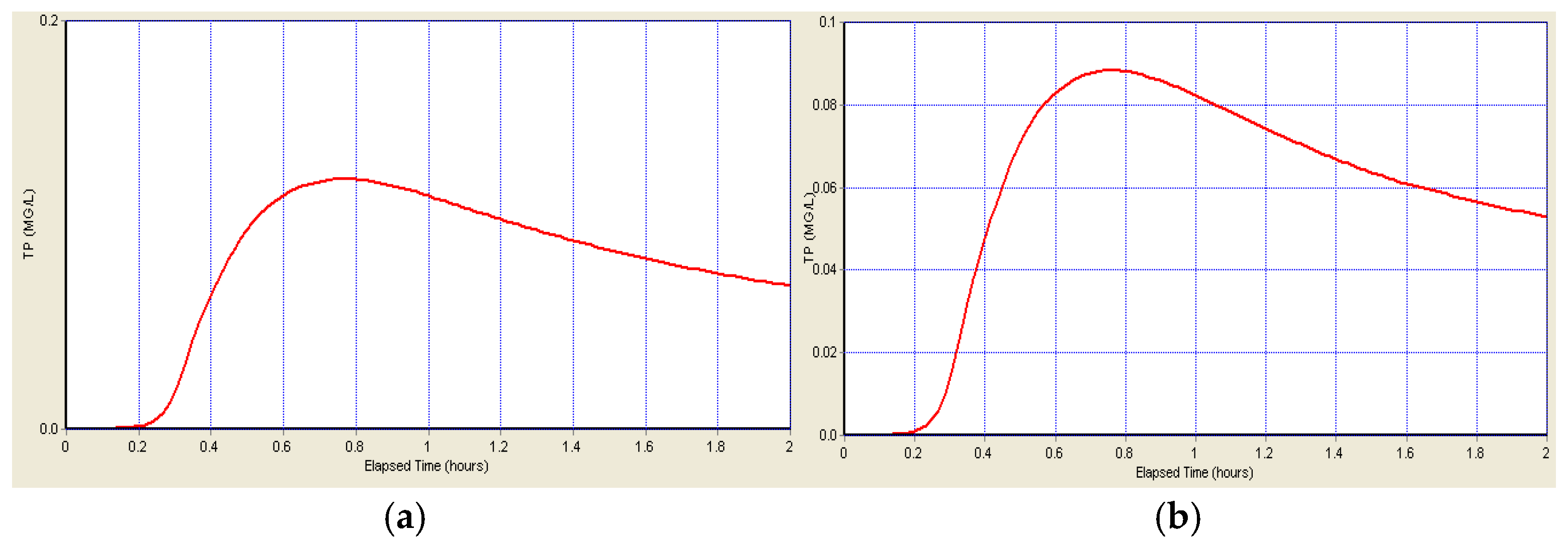
The TP concentration before and after adding the storage tank: (a) the TP concentration at the outlet node before adding the storage tank is 0.12 mg/L, and (b) the TP concentration at the outlet node after adding the storage tank is 0.085 mg/L.
Figure 12.
The TP concentration before and after adding the storage tank: (a) the TP concentration at the outlet node before adding the storage tank is 0.12 mg/L, and (b) the TP concentration at the outlet node after adding the storage tank is 0.085 mg/L.
Figure 13.
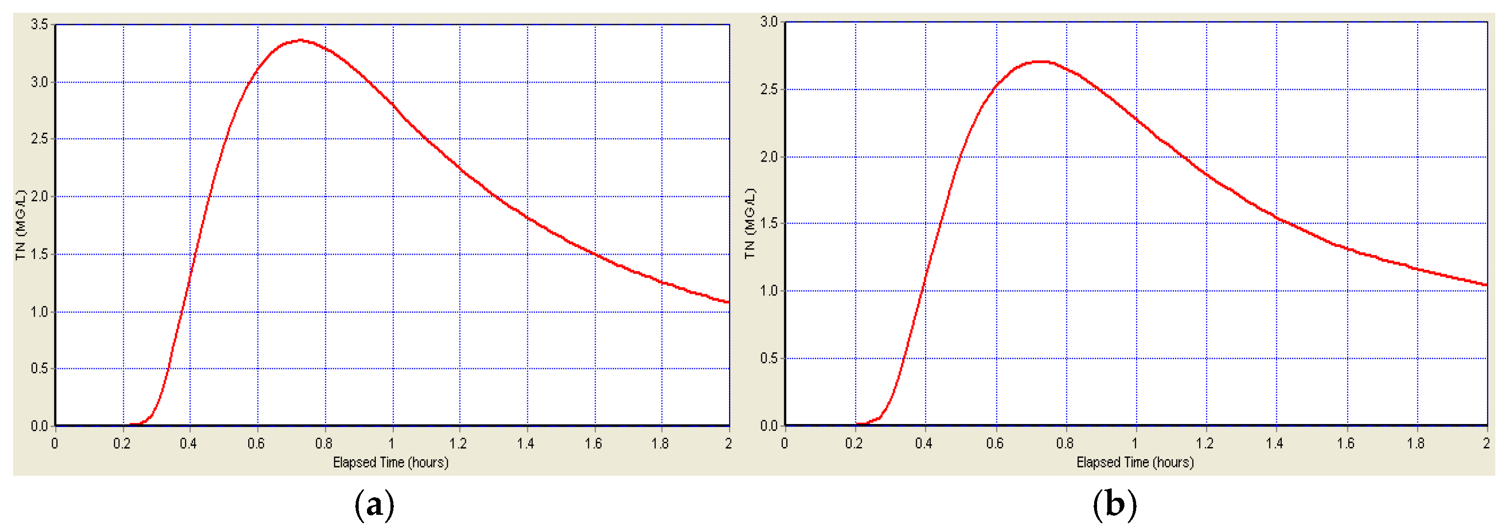
The TN concentration before and after adding the storage tank: (a) the TN concentration at the outlet node before adding the storage tank is 3.4 mg/L, and (b) the TN concentration at the outlet node after adding the storage tank is 2.6 mg/L.
Figure 13.
The TN concentration before and after adding the storage tank: (a) the TN concentration at the outlet node before adding the storage tank is 3.4 mg/L, and (b) the TN concentration at the outlet node after adding the storage tank is 2.6 mg/L.
Table 1.
Modeled production flow surface delineation and parameters.
Table 1.
Modeled production flow surface delineation and parameters.
| Division of Production Flow Surface | Roads | Roofs | Greenery |
|---|
| Constant runoff coefficient | 0.8 | 0.9 | - |
| Confluence parameter | 7 | 7 | 10 |
| Initial loss (m) | 0.002 | 0.002 | 0.012 |
| Initial penetration rate (mm/h) | - | - | 76.2 |
| Stable permeability (mm/h) | - | - | 3.18 |
| Attenuation rate (h − 1) | - | - | 6 |
Table 2.
Typical ranges of parameter values in runoff model simulations.
Table 2.
Typical ranges of parameter values in runoff model simulations.
| Type of Land Use | Permeable Surface | Impervious Surface | Plumbing |
|---|
| Low-density residential area | 0.10–0.20 | 0.010–0.015 | 0.011–0.013 |
| High-density residential area | 0.10–0.20 | 0.010–0.015 | 0.020–0.036 |
| Freeway | 0.10–0.20 | 0.010–0.015 | 0.011–0.013 |
Table 3.
Pollutant accumulation modeling on diverse land use surfaces.
Table 3.
Pollutant accumulation modeling on diverse land use surfaces.
| Parameter | TSS | COD | TN | TP |
|---|
Maximum road accumulation (kg/ha)
Road half-saturation and cumulative time (d) | 270 | 170 | 6.0 | 0.2 |
| 10 | 10 | 10 | 10 |
Maximum roof accumulation (kg/ha)
Roof half-saturation cumulative time (d) | 140 | 80 | 4.0 | 0.2 |
| 10 | 10 | 10 | 10 |
Maximum greenfield accumulation (kg/ha)
Greenfield half-saturation and cumulative time (d) | 60 | 40 | 10 | 0.6 |
| 10 | 10 | 10 | 10 |
Table 4.
Pollutant flushing coefficients on diverse land surfaces.
Table 4.
Pollutant flushing coefficients on diverse land surfaces.
| Item | TSS | COD | TN | TP |
|---|
| Roads | Scrub coefficient | 0.008 | 0.007 | 0.004 | 0.002 |
| Washout index | 1.8 | 1.8 | 1.7 | 1.7 |
| Sweeping removal rate | 70 | 70 | 70 | 70 |
| Roofing | Scrub coefficient | 0.007 | 0.006 | 0.004 | 0.002 |
| Washout index | 1.8 | 1.8 | 1.7 | 1.7 |
| Sweeping removal rate | 0 | 0 | 0 | 0 |
| Greenery | Scrub coefficient | 0.004 | 0.0035 | 0.002 | 0.001 |
| Washout index | 1.2 | 1.2 | 1.2 | 1.2 |
| Sweeping removal rate | 0 | 0 | 0 | 0 |
Table 5.
Calculation of storm intensity for the harbor area.
Table 5.
Calculation of storm intensity for the harbor area.
| t | P = 0.25 | P = 0.33 | P = 0.5 | P = 1 | P = 2 |
|---|
| 5 | 162.26 | 184.736 | 218.440 | 274.664 | 330.888 |
| 10 | 136.01 | 154.904 | 183.165 | 230.310 | 277.454 |
| 15 | 117.50 | 133.846 | 158.266 | 199.001 | 239.737 |
| 20 | 103.75 | 118.136 | 139.689 | 175.643 | 211.598 |
| 30 | 84.441 | 96.1683 | 113.713 | 142.982 | 172.250 |
| 45 | 66.540 | 75.7843 | 89.6107 | 112.675 | 135.740 |
| 60 | 55.237 | 62.9005 | 74.3763 | 93.5199 | 112.663 |
| 90 | 41.626 | 47.3986 | 56.0462 | 70.4719 | 84.8975 |
| 120 | 33.651 | 38.3227 | 45.314 | 56.9778 | 68.6412 |
| t | P = 3 | P = 5 | P = 10 | P = 20 | P = 50 |
| 5 | 363.777 | 405.212 | 461.436 | 517.660 | 591.984 |
| 10 | 305.032 | 339.776 | 386.921 | 434.065 | 496.387 |
| 15 | 263.566 | 293.587 | 334.323 | 375.058 | 428.908 |
| 20 | 232.63 | 259.127 | 295.081 | 331.035 | 378.564 |
| 30 | 189.371 | 210.941 | 240.210 | 269.478 | 308.169 |
| 45 | 149.232 | 166.23 | 189.294 | 212.359 | 242.849 |
| 60 | 123.861 | 137.969 | 157.113 | 176.257 | 201.563 |
| 90 | 93.3359 | 103.967 | 118.392 | 132.818 | 151.888 |
| 120 | 75.4639 | 84.0594 | 95.7228 | 107.386 | 122.804 |
Table 6.
Calibration results for hydrological parameters.
Table 6.
Calibration results for hydrological parameters.
| Model Parameter | Physical Significance | Rate Determination Outcome |
|---|
| N-imperv | Manning coefficient of impermeable area | 0.02 |
| N-perv | Manning coefficient of permeable area | 0.4 |
| S-imperv | Depression storage in impermeable area | 1 mm |
| S-perv | Puddle storage in permeable area | 10 mm |
| Max. infil | Maximum infiltration rate of Horton model | 80 mm/h |
| Min. infil | Minimum infiltration rate of Horton model | 3 mm/h |
| α | Attenuation constant | 2 h−1 |
| i | Landmark slope | 0.01 |
Table 7.
Parameterization of production and sink models.
Table 7.
Parameterization of production and sink models.
| Impervious Surface | Initial loss Dp/mm | Constant runoff coefficient C | Manning’s coefficient Ns |
| 1 | 0.8 | 0.02 |
| Permeable Surface | Initial loss Dp/mm | Primary filtration f0 | Stable percolation fc | Attenuation constant k | Manning’s coefficient Ns |
| 10 | 80 | 3 | 2 | 0.4 |
Table 8.
Sensitivity rankings of parameter indices affecting runoff volume.
Table 8.
Sensitivity rankings of parameter indices affecting runoff volume.
| Sensitivity Ranking | 1 | 2 | 3 | 4 | 5 |
|---|
| Indicator | C | Iimp | Fc | DP | Fk |
| Slope | −0.885 | −0.682 | 0.363 | 0.216 | −0.185 |
| Sensitivity Ranking | 6 | 7 | 8 | 9 | 10 |
| Indicator | Ns | Wc | F0 | Sc | NP |
| Slope | 0.137 | −0.135 | 0.115 | −0.004 | 0.003 |
Table 9.
Sensitivity rankings of parameter indices affecting runoff flood peak.
Table 9.
Sensitivity rankings of parameter indices affecting runoff flood peak.
| Sensitivity Ranking | 1 | 2 | 3 | 4 | 5 |
|---|
| Indicator | C | Iimp | Fc | DP | Fk |
| Slope | −0.863 | −0.545 | 0.174 | −0.162 | 0.149 |
| Sensitivity Ranking | 6 | 7 | 8 | 9 | 10 |
| Indicator | Ns | Wc | F0 | Sc | NP |
| Slope | −0.097 | 0.082 | 0.060 | 0.052 | −0.004 |
Table 10.
Parameters of rainwater infiltration ditch.
Table 10.
Parameters of rainwater infiltration ditch.
| Item | Dimension |
|---|
| Surface section size | Width × height = 1200 mm × 800 mm |
| Reinforced concrete cover plate | Thick = 60 mm. |
| Internal sand-free concrete rectangular ditch | 300 mm × 300 mm
Thick = 50 mm |
| Gravel filled externally | Particle size = 10~20 mm |
| The total length of the infiltration trench | 240 m |
| The slope of the underlying surface | 0.3% |
Table 11.
Parameters of rainwater storage tanks.
Table 11.
Parameters of rainwater storage tanks.
| Item | Data | Item | Data |
|---|
| Cylindrical steel–concrete substructures | Inner diameter 5 m | Pool edge water depth | 4.2 m |
| Top elevation | 0.8 m below the surface | Depth of water in the pond | 6.5 m |
| Pipe alignment bottom elevation | 2.0 m below the surface | DN1200 Water inlet pipe diameter | 80 m |
| Pump pit depth | 2 m | DN1000 Outlet pipe diameter | 50 m |
Table 12.
Results of the sensitivity analysis of LID facilities.
Table 12.
Results of the sensitivity analysis of LID facilities.
| Parameter | Peak Flood Flow | Volume of Runoff | Concentration of Pollutants | Combined Sensitivity |
|---|
| Rainfall intensity | Extremely high | High | Medium | 1 |
| Annual rainfall | High | High | Low | 2 |
| Permeable pavement permeability | Medium | High | Low | 3 |
| Soil permeability coefficient | Low | Medium | Low | 4 |
| Land use type | Low | Medium | High | 5 |
| Stormwater reuse rate | No direct effect | Low | Medium | 6 |
Table 13.
Analysis of the benefits of traditional stormwater management systems versus the LID systems.
Table 13.
Analysis of the benefits of traditional stormwater management systems versus the LID systems.
| Item | Traditional Rainwater Management System | LID Rainwater Management System |
|---|
| Stormwater reuse benefits | / | The annual rainwater collection amount is 1.82 × 10⁶ m3, replacing 30% of tap water and bringing a water cost reduction of CNY 50 million. |
| Flood control benefits | Flood flow reduction rate: 30% | Permeable pavements, ditch systems, and stormwater reservoirs reduce peak flows by 33.3%, 30%, and 50%. |
| Cost-effectiveness | Initial investment cost | CNY 12 million | CNY 1800 million |
| Annual maintenance cost | CNY 50 million | CNY 80 million |
| Combined annual benefits | CNY 30 million | CNY 150 million |
| Net present value (NPV) | CNY 200 million | CNY 1400 million |


