Article

The Role of Marketing Efforts in Enhancing Closed-Loop Supply Chains Under Recycling Competition

1
School of Management, University of Science and Technology of China, Hefei 230026, China
2
School of Business Administration, Anhui University of Finance and Economics, Bengbu 233030, China
*
Author to whom correspondence should be addressed.
Sustainability 2025, 17(6), 2531; https://doi.org/10.3390/su17062531
Submission received: 14 January 2025 / Revised: 23 February 2025 / Accepted: 7 March 2025 / Published: 13 March 2025

Abstract

:
In this study, we investigated a closed-loop supply chain system comprising manufacturers and retailers engaged in recycling competition. The manufacturer is the CLSC Stackelberg leader. By developing a Stackelberg model incorporating marketing, we analyzed the impact of marketing efforts by different agents on the entire system, specifically focusing on marketing conducted by the manufacturer, the retailer, and the centralized supply chain. Our findings reveal that the manufacturer consistently prefers the retailer to undertake marketing efforts. In contrast, the retailer favors the manufacturer to handle marketing when recycling competition intensity is low but prefers to conduct marketing themselves when the competition intensity is high. The extent of environmental harm under different models depends on the base demand: no marketing results in the least harm when the base demand is low, marketing by manufacturers minimizes harm when the base demand is moderate, and marketing by retailers causes the least harm when the base demand is high. Then, we performed a numerical analysis of the marketing cost-sharing contract and found that an appropriate sharing ratio consistently enhances the profitability of the entire supply chain. Finally, we examined the impact of a government subsidy for remanufacturing on supply chain performance and found that when recycling competition intensity is moderate, a government subsidy enhances supply chain performance more effectively.

1. Introduction

With the growing awareness of environmental protection and sustainable development, an increasing number of enterprises are recycling end-of-use products and materials for remanufacturing, integrating these processes into closed-loop supply chains (CLSCs) alongside the traditional forward supply chain. The European Remanufacturing Network estimates that the remanufacturing market in Europe will grow to EUR 90 billion by 2030, tripling the EUR 30 billion market in 2015 [1]. In China, the government has implemented a series of policies and regulations to support the growth of the remanufacturing industry [2]. The size of China’s remanufacturing sector reached USD 3.28 trillion in 2023 [3]. Many leading companies are increasingly prioritizing the recycling and remanufacturing of used products. For instance, Kodak increased its remanufactured production by 51% from 2016 to 2022 to meet its sustainability goals [4]. HP has also introduced a reuse and recycling program for unwanted equipment and printing consumables [5]. Remanufacturing involves the specialized repair and restoration of used items such as automotive parts, engineering instruments, and machine tools [6,7]. The remanufactured products meet the same quality and performance standards as new ones while achieving significant energy, material, and cost savings. In addition, the process of recycling and remanufacturing used products benefits the environment by recycling waste and reducing carbon emissions. Remanufacturing can achieve near-zero solid waste generation and reduce air pollution emissions by over 80%, making it an effective approach to maximizing resource utilization and protecting the ecological environment [8].
While in most industries the production process of remanufacturing can only be accomplished by manufacturers, the recycling process of remanufacturing can also be conducted by retailers. Retailers have the natural advantage of being closer to consumers, who are increasingly interested in recycling used products [9,10,11]. As remanufacturing technologies continue to mature, the value of used products has gradually increased, intensifying recycling competition between manufacturers and retailers. The collection of used products by retailers introduces competition with manufacturers’ collection efforts. However, manufacturers can also purchase recycled products from retailers and recyclers, fostering a cooperative dynamic process alongside the competition. For instance, Apple’s device exchange program operates through both online platforms and offline retail store channels [12].
In a closed-loop supply chain, consumer purchasing behavior is influenced not only by the price and value of a product but also by a firm’s advertising and marketing efforts. Consumers are often resistant to purchasing remanufactured products because they are concerned about their quality [13]. Therefore, through specific marketing tools, such as explanations of remanufacturing principles and processes on content platforms, consumers can develop greater confidence in the quality of remanufactured products [14,15]. In addition, consumers’ green attributes and their concern for green products are often important factors in their interest in remanufactured products [16]. Advertising is an important way to raise their awareness of green products [17]. Advertising that promotes the environmental benefits of remanufactured products can resonate with consumers and increase their willingness to purchase [18,19,20]. Such marketing efforts can be undertaken not only by manufacturers to promote their brand image and environmental values but also by retailers, who maintain closer connections with consumers [21,22]. Marketing often incurs certain costs, such as producing remanufactured content, purchasing traffic on web content platforms, and renting paid smart marketing software. For instance, to promote its “Move to Zero” initiative, Nike partnered with Ant Group to launch a green energy campaign. They introduced the “Nike Old Shoes New Life” mini program on Alipay, enabling consumers to recycle their old shoes through the app. Participants earn corresponding Ant Forest green energy points, allowing them to unlock new green achievements and contribute to environmental sustainability [23].
Cooperation among supply chain members plays a crucial role in building a sustainable supply chain. Empirical studies have shown that cooperation enhances supply chain performance by enabling the integration of internal and external resources, thereby promoting more sustainable development [24]. In this article, we also explore the marketing cost-sharing contract between manufacturers and retailers.
The intricate interplay of competition and cooperation between manufacturers and retailers in a recycling-driven closed-loop supply chain inspired our investigation into determining the most appropriate marketing agents for such a system. Based on the above observations, in this study, we utilized the Stackelberg game model to construct a closed-loop supply chain model consisting of a manufacturer and a retailer. In the forward supply chain, the manufacturer sells goods to consumers through retailers; in the reverse supply chain, the manufacturer and retailers competitively recycle used products from consumers, and the manufacturer also buys used products from retailers at a buyback price. In this paper, we discuss four scenarios of the model depending on the marketing agent: (1) no marketing efforts (Model B), (2) a manufacturer exerting marketing efforts (Model M), (3) a retailer exerting marketing efforts (Model R), and (4) a centralized supply chain exerting marketing efforts (Model C). Based on these, we pose the following questions:
(1)
When comparing the first three models, which is the preferred option for retailers, manufacturers, and the overall supply chain? How does the intensity of recycling competition influence their preferences?
(2)
How do consumer surplus and environmental damage levels vary across different models?
(3)
Can a marketing cost-sharing contract be implemented to optimize the profits for manufacturers, retailers, and the overall supply chain?
(4)
What impact will government subsidy for remanufacturing have on the supply chain?
Our findings reveal that in the first three models, the manufacturer consistently prefers the retailer to undertake marketing efforts, regardless of the intensity of recall competition. However, when recycling competition is weak, the retailer prefers the manufacturer to handle marketing efforts, whereas under strong recycling competition, the retailer is willing to take on the marketing efforts themselves. The consumer surplus is consistently highest when the retailer undertakes the marketing efforts. The environmental damage associated with different modes depends on the base demand. When the base demand is high, the retailer’s marketing efforts result in lower environmental damage. Conversely, when the base demand is low, marketing efforts by the manufacturer lead to lower environmental damage. Additionally, we found that a marketing cost-sharing contract consistently enhances the profitability of the entire supply chain. This cost-sharing arrangement can be naturally achieved when the manufacturer undertakes the marketing efforts. Finally, a government subsidy for remanufacturing is generally beneficial for the remanufacturer, but it can negatively impact the profit of the retailer. When the intensity of recycling competition is moderate, a government subsidy can more effectively optimize the overall profit of the supply chain.
The main innovations of this paper are as follows. Enhancing the management of closed-loop supply chains facilitates resource conservation, minimizes emissions and pollution, and promotes the sustainable development of both enterprises and society. A significant number of studies have been conducted on marketing management within closed-loop supply chains. However, there is a lack of study examining the impact of competition within recycling channels on the marketing model. Competition in recycling channels is prevalent across various industries and significantly influences the recycling and marketing strategies of supply chain members. This, in turn, has a profound effect on both supply chain optimization and environmental sustainability. Therefore, this study explores the impact of recycling competition on the marketing model in closed-loop supply chains, contributing to the theoretical development of closed-loop supply chain management.
The remainder of the article is organized as follows: Section 2 reviews the relevant literature. Section 3 presents the model and hypotheses. Section 4 provides the optimal solutions of the model. Section 5 analyzes the results. In Section 6, through numerical studies, the following is carried out: in Section 6.1, we examine strategic preferences and environmental damage; in Section 6.2, we explore the impact of a cost-sharing model on supply chain profits; in Section 6.3, we make an extended analysis of the situation where production costs are not zero; and in Section 6.4, we consider the impact of a government subsidy for remanufacturing on supply chain performance. Finally, Section 7 summarizes our findings and outlines future research directions. All proof is provided in Appendix A.

2. Literature Review

In this section, we review the relevant literature across four main areas: (1) recycling channel management in CLSCs, (2) channel competition in CLSCs, (3) marketing efforts in CLSCs, and (4) consumer behavior in the circular economy.

2.1. Recycling Channel Management in CLSCs

Recycling channel management in CLSCs is a crucial research direction. As a pioneering work, Savaskan et al. [25] examined the selection of appropriate entities for recycling used products within a closed-loop supply chain. They analyzed three scenarios: (1) manufacturers managing recycling directly, (2) retailers handling recycling, and (3) outsourcing recycling to third-party entities. Their findings highlight that retailers are better suited to act as recyclers of used products. Similarly, several other studies have explored the issue of optimal subjects for recycling activities under different conditions. Alegoz et al. [26] used a two-stage model to depict CLSCs, incorporating firms’ discount factors and environmental sensitivities, and outlined conditions for manufacturers to outsource recycling to third parties. Zheng et al. [27] analyzed the optimal recycling channel choice in a dual-channel structure comprising a direct sales channel and a traditional retail channel, finding that both the manufacturer and the retailer prefer to handle recycling independently. Giri et al. [28] developed a model incorporating a dual forward channel and a dual recycling channel structure, comprising a traditional retail platform and an e-platform. The model is used to derive optimal pricing and recycling decisions under varying power structures. Atasu et al. [29] analyzed the influence of the collection cost structure on the optimal selection of the recycling channel. The authors noted that the manufacturer’s optimal choice of reverse channel is influenced by how the collection cost impacts the retailer’s sales and quantity decisions. Chuang et al. [30] explored the optimal recycling channel selection for manufacturers with short product life cycles and volatile demand. Cheng and Wang [31] investigated the optimal recycling channel selection in a closed-loop supply chain under conditions where consumers are uncertain about the quality of remanufactured products. Ziaei et al. [32] investigated pricing and collection rate decisions in closed-loop supply chains (CLSCs) under a reward–penalty mechanism (RPM). They found that a coordinated structure with a two-part tariff contract outperforms decentralized models in collection rates and profitability. Yu et al. [33] developed differential game models for a dual-channel closed-loop supply chain (DCCLSC) under non-cooperation, partial cooperation, and full cooperation scenarios, analyzing recycling and pricing decisions from a dynamic perspective. Li et al. [34] proposed an optimization model aimed at minimizing the total network cost, along with the sum of carbon rewards and penalties, when selecting facility locations and transportation routes between network nodes.
There are also empirical studies that examine management in CLSCs. Confente et al. [35] conducted an experimental study to examine how lenient return policies reduce consumers’ perceived risk and influence their purchase intention for remanufactured products across brick-and-mortar and online channels. Their study found that a lenient return policy significantly boosts purchase intention and that consumers perceive similar risk levels for remanufactured products sold through both channels. Bhatia et al. [36] used survey data from Indian manufacturing firms and identified key capabilities for closed-loop supply chains (CLSCs): information technology and organizational learning as the lower order and internal integration, demand management, and product design as the higher order. Martin et al. [37] found that intellectual property, operational assets, and remanufacturing frequency significantly influence the remake-versus-buy decision.
Our study considers a competitive recycling scenario in a closed-loop supply chain where both manufacturers and retailers have recycling capabilities.

2.2. Channel Competition in CLSCs

In this subsection, we review articles from the literature that address channel competition in closed-loop supply chains, focusing on two aspects: competition in forward supply chains and competition in recycling channels within reverse supply chains.
The following literature addresses the issue of channel competition in forward supply chains [38,39,40,41,42]. Zheng et al. [38] examined the impact of forward supply channel competition and power structures on a two-channel closed-loop supply chain. Their findings reveal that, under positive channel competition, each supply chain member shows a preference for assuming a leadership role. Jalapathy and Unnissa [39] analyzed product pricing in the context of competition between new and remanufactured products. Qiang [40] examined the optimal product quality and quantity in the context of market share competition among remanufacturers in a two-phase CLSC. Additionally, their analysis addressed the impact of remanufactured product design and consumer perceptions of remanufactured products on profits and market share. Zhang and Ren [41] constructed a closed-loop supply chain consisting of remanufacturers, original manufacturers, and third-party collection platforms in which they accounted for demand competition. Hosseini et al. [42] analyzed the competition between two dealers for used product services and examined the incentives provided to suppliers under such competitive conditions.
The following studies focused on recycling competition within the reverse channel [43,44,45,46,47,48,49]. Huang et al. [43] examined a closed-loop supply chain comprising manufacturers, retailers, and third-party collection platforms, where retailers and third-party platforms compete for the recycling of used products. They compared the performance of supply chains under competitive recycling with those using a single-channel recycling approach and found that dual-channel recycling outperformed under specific parameters. He et al. [44] compared the recycling efficiency of decentralized recovery models involving retailers and manufacturers with that of centralized models and proposed two coordination mechanisms to improve the performance of decentralized recovery models. Wang et al. [45] investigated whether manufacturers should establish a fully integrated closed-loop supply chain or outsource recycling activities to retailers in a competitive recycling market. Zhou et al. [46] analyzed the equilibrium outcomes of recycling channels under the leadership of electric vehicle manufacturers and electric vehicle recyclers, taking into account the competition between automotive recyclers and third-party recyclers. Feng et al. [47] compared decentralized and centralized models in closed-loop supply chains, considering recycling competition and differences in recycling quality. Zhang et al. [48] found that enterprises in the supply chain will opt for a competitive recycling model only when the intensity of competition exceeds a specific threshold. He et al. [49] examined the optimal collection strategies under monopoly, duopoly, and mixed competition, considering customer sensitivity to the convenience of returning discarded products. Competition for recycled products is prevalent in practice. For example, common recycling channels for Apple products often include third-party platforms, offline stores, and official websites. To better align with real-world scenarios, our literature considered the competition between manufacturers and retailers in the recycling process.

2.3. Marketing Efforts in CLSCs

The impact of marketing activities has also been extensively examined in the closed-loop supply chain research literature [50,51,52,53,54,55,56]. Taleizadeh et al. [50] compared the marketing efforts of different supply chain agents in a closed supply chain, consisting of a manufacturer’s direct sales channel and a traditional retail channel, but did not address the channel competition involved. Hong and Guo [51] compared three different contracts between manufacturers and retailers in a closed-loop supply chain with social responsibility considerations, including pure price contracts, green marketing cost-sharing contracts, and two-part tariff contracts. Li et al. [52] examined the case of retailer cost sharing for the manufacturer’s greening inputs in a closed supply chain, where the retailer handles marketing efforts, and the manufacturer focuses on product greening. They compared this with the scenario where the manufacturer shares the marketing costs with the retailer. Gao et al. [53] analyzed optimal decisions for pricing, recycling efforts, and marketing efforts under three power structures in a closed-loop supply chain. These structures include manufacturer-dominated, retailer-dominated, and vertical Nash. Hu et al. [54] compared different sales effort models under the influence of network externalities, including no marketing efforts, retailers making marketing efforts, and manufacturers making marketing efforts. They accounted for network externalities in the forward channel but did not address competition in the recycling channel. Ma et al. [15] analyzed the optimal recycling and marketing efforts under four reverse channel structures where retailers are responsible for marketing efforts considering fairness concerns. Asghari et al. [55] developed a new optimization model for direct-sales closed-loop supply chains that incorporates both pricing and advertising decisions.
However, the aforementioned studies that address marketing in closed-loop supply chains overlook competition in the recycling process. This study aimed to explore how competition in the recycling channel influences the choice of optimal marketing strategy.

2.4. Consumer Behavior in the Circular Economy

Consumer behavior is also particularly important for the management of closed supply chains. Through an empirical analysis of the relationship between online reviews and the sale of remanufactured products, Zhai et al. [56] found that review length and review valence have positive influences on remanufactured product sales. Chen et al. [57] experimentally validated that consumers employ distinct selection mechanisms when choosing among new, remanufactured, and refurbished products and further explored the relationship between these mechanisms and the inherent attributes of the products themselves. Through questionnaire surveys and data analysis, Lakatos et al. [58] found that consumers’ positive attitudes toward green products and their understanding of green attributes are significant predictors of satisfaction with green products. Fu et al. [59] used meta-analytic structural equation modeling (MASEM) to analyze consumers’ willingness to pay (WTP) for circular products, finding that personal norms had the strongest positive correlation with WTP. Zhang et al. [60] examined factors influencing consumers’ intention to buy remanufactured products and found that attitude, subjective norms, and perceived behavioral control significantly affect intention. Additionally, environmental concern positively impacts these factors, while perceived risk negatively influences attitude and adoption intention. Chinen et al. [61] used a structural equation model (SEM) to analyze respondents’ acceptance, purchase intention, and willingness to pay for remanufactured EV batteries. The results reveal that price consciousness and perceived benefits directly influence purchase intention. Chun et al. [62] identified perceived risk, consumer innovativeness, and price as critical factors influencing consumer participation in circular consumption.

3. Problem Description

We considered a CLSC that included a manufacturer and a retailer. The manufacturer produces a product with virgin and used materials, which can be collected by themselves and purchased from the retailer at a buyback price b . We define k as the cost saving per unit achieved by recycling used materials. The retailer purchases the product at a wholesale price w and sells it to consumers at a price p . The model’s notations are presented in Table 1.
In the recycling market, the manufacturer and retailer compete to collect the partial materials of used products from consumers. A parameter, α , is used to illustrate the intensity of the competition between them. Consistent with Huang et al. [43] and Hong et al. [51], we assume members’ recycling investments have a symmetric influence on each other as follows:
ζ m = ( I m α   I r ) / c ,     ζ r = ( I r α   I m ) / c ,
where 0 ζ m + ζ r < 1 , and c is the recycling cost parameter, which is assumed to be sufficiently large. Then, the investment cost can be presented as follows:
I m = c ζ m 2 + α   ζ r 2 1 α 2 ,     I r = c ( ζ r 2 + α   ζ m 2 1 α 2 ) .
Following Taleizadeh et al. [50], the market demand can be increased by exerting the marketing efforts at level y , and the incurred cost is ( 1 / 2 ) z   y 2 , where z is the marketing cost coefficient. Hence, the demand can be expressed as follows:
D = d β   p + y ,
where d pertains to the market base, and β is the price–demand coefficient. The other assumptions for this paper are listed as follows:
(1)
We assume the products produced by virgin and recycled materials have the same utility to consumers and that all products are sold at the same price [50,63]. This assumption holds true particularly in specific industries, such as printers and engines, where remanufacturing enables recycled old products to achieve performance levels that are either on par with or even surpass those of new products. For example, KODAK Remanufactured Toner Cartridges are made by recycling empty, used, original HP, Brother, or Samsung toner cartridges. They look and feel just like original cartridges. The print quality also matches or exceeds that of the originals, and most consumers do not know that the new products they buy contain “remanufactured parts” [64]. In another example, Caterpillar demonstrates its commitment to sustainability by assembling recycled components into new parts while strictly adhering to the original equipment manufacturer’s (OEM) performance specifications. These parts undergo rigorous testing to ensure they meet the same high standards as new Caterpillar components. Furthermore, they are backed by the same warranty, offering the same reliability and durability as newly manufactured parts, thus ensuring consistent quality and performance [65].
(2)
The unit producing cost is assumed to be 0 [54,66].
(3)
We assume α > k 2 4 + k 2 and c > k 2 ( 1 α 2 ) 4 α 2 to ensure that recycling competition is sufficiently strong; otherwise, recycling volumes could surpass new product production, which would be factually inaccurate [52,62].
(4)
We assume z > 2 c α 2 4 c α 2 β k 2 β 2 ( 1 α 2 + α 3 α 5 ) to ensure that the cost of the promotion is high enough to ensure the existence of an optimal marketing intensity solution [50].

4. Model Formulation and Solution

We aim to examine the impact of the marketing efforts of different supply chain members on CLSCs considering recycling competition. Hence, four models are detailed as follows: The first model is our base model, in which we do not incorporate marketing efforts. In the second and third models, we examine separately the situation when the manufacturer exerts marketing efforts and when the retailer exerts marketing efforts. In the fourth model, to compare the performance of centralized and decentralized supply chains, we study the centralized supply chain case with marketing efforts.

4.1. Model B (Without Marketing Efforts)

In this model, neither the manufacturer nor the retailer exerts marketing efforts in the CLSC system. The decision sequence can be described as follows: First, the manufacturer determines the recycling efforts ζ m B , the buyback price b B , and the wholesale price w B . Then, the retailer sets the recycling efforts ζ r B and the product price p B . The demand function is the following:
D B = d β   p B ,
Now, the profit functions of the manufacturer and the retailer can be expressed as follows:
π m B = w B + k   ζ m B + ζ r B b B   ζ r B   D B c ζ m B 2 + α   ζ r B 2 1 α 2 ,
π r B = p B + b B   ζ r B   D B c ζ r B 2 + α   ζ m B 2 1 α 2 .
With the aforementioned expression, we have Proposition 1.
Proposition 1. 
In Model B, the optimal decisions of the manufacturer and retailer are the following:
ζ m B = d k α ( 1 α 2 ) 8 c α k 2 ( 1 α ) ( 1 + α ) 2 β ,
b B = k α ,
w B = d ( 4 c α 2 + k 2 ( 1 α 2 α 2 + α 3 + α 4 ) β ) α β ( 8 c α k 2 ( 1 α ) ( 1 + α ) 2 β ) ,
ζ r B = d k ( 1 α 2 ) 8 c α k 2 ( 1 α ) ( 1 + α ) 2 β ,
p B = d ( 6 c α k 2 ( 1 α ) ( 1 + α ) 2 β ) β ( 8 c α k 2 ( 1 α ) ( 1 + α ) 2 β ) .
In this model, with the optimal decisions in Proposition 1, the optimal demand and the profits of the manufacturer, the retailer, and the total supply chain can be derived as follows:
D B = 2 c d α 8 c α k 2 ( 1 α ) ( 1 + α ) 2 β ,
π m B = c d 2 α β ( 8 c α k 2 ( 1 α ) ( 1 + α ) 2 β ) ,
π r B = c d 2 ( 4 c α 2 k 2 ( 1 α 2 + α 3 α 5 ) β ) β ( 8 c α k 2 ( 1 α ) ( 1 + α ) 2 β ) 2 ,
π S C B = c d 2 ( 12 c α 2 + k 2 ( 1 α + α 4 + α 5 ) β ) β ( 8 c α + k 2 ( 1 + α ) ( 1 + α ) 2 β ) 2 .
The consumer surplus and environmental damage are the following:
C S B = 2 c 2 d 2 α 2 ( 8 c α + k 2 ( 1 + α ) ( 1 + α ) 2 β ) 2 ,
E D B = 2 c d α ( 8 c α + d k ( 1 + α ) ( 1 + α ) 2 + k 2 ( 1 + α ) ( 1 + α ) 2 β ) θ ( 8 c α + k 2 ( 1 + α ) ( 1 + α ) 2 β ) 2 ,

4.2. Model M (Manufacturer Invests in Marketing Efforts)

In this model, the manufacturer exerts marketing efforts in the CLSC system. The decision sequence can be described as follows: First, the manufacturer determines the recycling efforts ζ m M , the buyback price b M , the wholesale price w M , and the marketing effort intensity y M . Then, the retailer sets the recycling efforts ζ r M and the product price p M . The demand function is the following:
D M = d β   p M + y M ,
Now, the profit functions of the manufacturer and the retailer can be expressed as follows:
π m M = w M + k   ζ m M + ζ r M b M   ζ r M   D M c ζ m M 2 + α   ζ r M 2 1 α 2 1 2   z   y M 2 ,
π r M = p M + b M   ζ r M   D M c ζ r M 2 + α   ζ m M 2 1 α 2 .
With the aforementioned expression, we have Proposition 2.
Proposition 2. 
In Model M, the optimal decisions of the manufacturer and retailer are the following:
ζ m M = d k z ( 1 α 2 ) β z b 2 α 2 b k k 2 1 α 2 β 2 c ( 2 8 z β ) ,
b M = k α ,
w M = d z ( 4 c α 2 + k 2 ( 1 α 2 α 2 + α 3 + α 4 ) β ) α ( k 2 z 1 + α 1 + α 2 β 2 2 c α ( 1 4 z β ) ) ,
y M = 2 c d α k 2 z 1 + α 1 + α 2 β 2 2 c α ( 1 4 z β ) ,
ζ r M = d k z ( 1 α 2 ) β k 2 z 1 + α 1 + α 2 β 2 2 c α ( 1 4 z β ) ,
p M = d z ( 6 c α + k 2 ( 1 + α ) ( 1 + α ) 2 β ) k 2 z 1 + α 1 + α 2 β 2 2 c α ( 1 4 z β ) .
In this model, with the optimal decisions in Proposition 2, the optimal demand and the profits of the manufacturer, the retailer, and the total supply chain can be derived as follows:
D M = 2 c d z α β k 2 z 1 + α 1 + α 2 β 2 2 c α ( 1 4 z β ) ,
π m M = c d 2 z α k 2 z 1 + α 1 + α 2 β 2 2 c α ( 1 4 z β ) ,
π r M = c d 2 z 2 β ( 4 c α 2 k 2 ( 1 α 2 + α 3 α 5 ) β ) ( k 2 z 1 + α 1 + α 2 β 2 2 c α ( 1 4 z β ) ) 2 ,
π S C M = c d 2 z ( k 2 z ( 1 α + α 4 + α 5 ) β 2 + 2 c α 2 ( 1 + 6 z β ) ) ( k 2 z ( 1 + α ) ( 1 + α ) 2 β 2 + 2 c α ( 1 + 4 z β ) ) 2 .
The consumer surplus and environmental damage are the following:
C S M = 2 c 2 d 2 z 2 α 2 β 2 ( k 2 z ( 1 + α ) ( 1 + α ) 2 β 2 + 2 c α ( 1 + 4 z β ) ) 2 ,
E D M = 2 c d z α β ( k z ( 1 + α ) ( 1 + α ) 2 β ( d + k β ) + 2 c α ( 1 + 4 z β ) ) θ ( k 2 z ( 1 + α ) ( 1 + α ) 2 β 2 + 2 c α ( 1 + 4 z β ) ) 2 ,

4.3. Model R (Retailer Invests in Marketing Efforts)

In this model, the retailer exerts marketing efforts in the CLSC system. The decision sequence can be described as follows: First, the manufacturer determines the recycling efforts ζ m R , the buyback price b R , and the wholesale price w R . Then, the retailer sets the recycling efforts ζ r R , the product price p R , and the marketing effort intensity y R . The demand function is the following:
D R = d β   p R + y R ,
Now, the profit functions of the manufacturer and the retailer can be expressed as follows:
π m R = w R + k   ζ m R + ζ r R b R   ζ r R   D R c ζ m R 2 + α   ζ r R 2 1 α 2 ,
π r R = p R + b R   ζ r R   D R c ζ r R 2 + α   ζ m R 2 1 α 2 1 2   z   y R 2 .
With the above expression, we have Proposition 3.
Proposition 3. 
In Model R, the optimal decisions of the manufacturer and retailer are the following:
ζ m R = d k z α ( 1 α 2 ) β k 2 z ( 1 + α ) ( 1 + α ) 2 β 2 + 4 c α ( 1 + 2 z β ) ,
b R = k α ,
w R = d ( k 2 z ( 1 α 2 α 2 + α 3 + α 4 ) β 2 + 2 c α 2 ( 1 + 2 z β ) ) α β ( k 2 z ( 1 + α ) ( 1 + α ) 2 β 2 + 4 c α ( 1 + 2 z β ) ) ,
ζ r R = d k z ( 1 + α 2 ) β k 2 z ( 1 + α ) ( 1 + α ) 2 β 2 + 4 c α ( 1 + 2 z β ) ,
p R = d ( k 2 z ( 1 + α ) ( 1 + α ) 2 β 2 + 2 c α ( 1 + 3 z β ) ) k 2 z ( 1 + α ) ( 1 + α ) 2 β 3 + 4 c α β ( 1 + 2 z β ) ,
y R = 2 c d α k 2 z ( 1 + α ) ( 1 + α ) 2 β 2 + 4 c α ( 1 + 2 z β ) .
In this model, with the optimal decisions in Proposition 3, the optimal demand and the profits of the manufacturer, the retailer, and the total supply chain can be derived as follows:
D R = 2 c d z α β k 2 z ( 1 + α ) ( 1 + α ) 2 β 2 + 4 c α ( 1 + 2 z β ) ,
π m R = c d 2 z α k 2 z ( 1 + α ) ( 1 + α ) 2 β 2 + 4 c α ( 1 + 2 z β ) ,
π r R = c d 2 z ( k 2 z ( 1 + α 2 α 3 + α 5 ) β 2 + 2 c α 2 ( 1 + 2 z β ) ) ( k 2 z ( 1 + α ) ( 1 + α ) 2 β 2 + 4 c α ( 1 + 2 z β ) ) 2 ,
π S C R = c d 2 z ( k 2 z ( 1 α + α 4 + α 5 ) β 2 + 6 c α 2 ( 1 + 2 z β ) ) ( k 2 z ( 1 + α ) ( 1 + α ) 2 β 2 + 4 c α ( 1 + 2 z β ) ) 2 .
The consumer surplus and environmental damage are the following:
C S R = 2 c 2 d 2 z 2 α 2 β 2 ( k 2 z ( 1 + α ) ( 1 + α ) 2 β 2 + 4 c α ( 1 + 2 z β ) ) 2 ,
E D R = 2 c d z α β ( k z ( 1 + α ) ( 1 + α ) 2 β ( d + k β ) + 4 c α ( 1 + 2 z β ) ) θ ( k 2 z ( 1 + α ) ( 1 + α ) 2 β 2 + 4 c α ( 1 + 2 z β ) ) 2 ,

4.4. Model C (Centralized Supply Chain Exerts Marketing Efforts)

In this section, we integrate the manufacturer and the retailer into a single decision-making entity who determines the recycling efforts in the two channels ζ m C and ζ r C , the product price p C , and marketing effort level y C . The demand function is the following:
D C = d β   p C + y C ,
Now, the profit functions of the centralized supply chain can be expressed as follows:
π S C C = p C + k   ζ m C + ζ r C   D C c ζ m C 2 + α   ζ r C 2 1 α 2 c ζ r C 2 + α   ζ m C 2 1 α 2 1 2   z   y c 2 .
Proposition 4. 
In Model C, the optimal decisions of the centralized supply chain are the following:
ζ m C = ζ r C = d k z ( 1 α ) β 2 k 2 z ( 1 + α ) β 2 + c ( 2 + 4 z β ) ,
p C = d z ( c + k 2 ( 1 + α ) β ) k 2 z ( 1 + α ) β 2 + c ( 1 + 2 z β ) ,
y C = c d k 2 z ( 1 + α ) β 2 + c ( 1 + 2 z β ) .
In this model, with the optimal decisions in Proposition 4, the optimal demand and the profit of the centralized supply chain can be derived as follows:
D C = c d z β k 2 z ( 1 + α ) β 2 + c ( 1 + 2 z β ) ,
π S C C = c d 2 z 2 k 2 z ( 1 + α ) β 2 + c ( 2 + 4 z β ) .
The consumer surplus and environmental damage are the following:
C S C = c 2 d 2 z 2 β 2 2 ( k 2 z ( 1 + α ) β 2 + c ( 1 + 2 z β ) ) 2 ,
E D C = c d z β ( k z ( 1 + α ) β ( d + k β ) + c ( 1 + 2 z β ) ) θ ( k 2 z ( 1 + α ) β 2 + c ( 1 + 2 z β ) ) 2 .

5. Discussion

In this section, we compare the equilibrium results for the different models in Section 4 and analyze the effect of key parameters.
Corollary 1. 
The optimal wholesale price and sales price in different models are as follows: w M > w R > w B , p C > p R > p M > p B .
Corollary 1 demonstrates that (1) the sales price is highest in the centralized supply chain model, whereas it is lowest in the benchmark model without marketing efforts. This suggests that regardless of which supply chain member undertakes the marketing efforts, the associated costs are ultimately passed on to the consumer through higher product prices. (2) Compared to the model where the manufacturer undertakes the marketing efforts, the model with retailer-led marketing results in a lower wholesale price but a higher sales price. When the manufacturer undertakes marketing, to cover marketing expenses and enhance its own profitability, the manufacturer raises the wholesale price, which in turn incentivizes the retailer to set lower selling prices to achieve significant increases in demand. In contrast, when the retailer handles the marketing efforts, it directly targets consumers to boost sales and profitability. Retailers, being closer to the end consumer, can tailor marketing strategies better to consumer preferences. To support this, manufacturers are incentivized to keep the wholesale price lower to encourage retailers’ promotional activities. The retailers, in turn, raise the sales price to recover marketing costs and maximize their margins.
Corollary 2. 
The optimal buyback price of the recycling materials and optimal recycling efforts of the manufacturer and retailer are as follows: b M = b R = b B , ζ m M > ζ m R > ζ m B , ζ r R > ζ r M > ζ r B .
Corollary 2 states that (1) the selection of the supply chain member responsible for implementing recycling efforts does not influence the optimal price of recycled materials. (2) Compared to the scenario where no marketing efforts are undertaken, both the manufacturer and retailer’s recycling efforts increase when marketing efforts are implemented. Marketing increases profitability by raising product sales, providing firms with more resources to invest in recycling efforts. Both the manufacturer and retailer see the value of recycling as a way to reduce raw material costs and improve their long-term competitiveness. (3) Supply chain members that implement marketing efforts also tend to enhance their recycling efforts, indicating a positive correlation between marketing initiatives and environmental responsibility.
Corollary 3. 
The optimal marking effort level and demand in different models are as follows: d C > d R > d M > d B , y C > y R > y M .
Corollary 3 demonstrates that (1) demand consistently increases with the adoption of marketing efforts, with the highest marketing intensity observed in a centralized supply chain, resulting in the highest demand. (2) The marketing investment is greater when retailers undertake marketing efforts compared to manufacturers. Consequently, market demand is also higher when retailers engage in promotions than when manufacturers do. This is because retailers are the final touchpoint in the supply chain, making them more invested in the success of marketing initiatives that directly impact consumer purchasing decisions.
Corollary 4. 
The optimal profits of the manufacturer and the entire supply chain in different models are as follows:   π m R > π m M > π m B , π S C C > π S C R > π S C M > π S C B .
Corollary 4 demonstrates that (1) both the manufacturer and the retailer’s marketing efforts lead to increased profits for the manufacturer compared to a scenario with no marketing efforts. However, the manufacturer prefers the retailer to undertake the marketing efforts rather than handling marketing themselves. (2) Profit for the entire supply chain is highest under a centralized structure, driven by the higher prices and greater marketing intensity enabled by centralized decision making. Among the remaining three models, when the retailer conducts marketing efforts, the benefits of marketing are more directly aligned with their interests due to their closer connection to consumers, resulting in higher marketing intensity and, consequently, elevated prices. The retailer’s preference for marketing models is demonstrated through a numerical example in the next section.
Corollary 5. 
The optimal consumer surplus and environmental damage in the first three models are the following:
(1)
S C R > S C M > S C B ;
(2)
When  d < d 1 , then  E D R > E D M > E D B ; when  d 1 < d < d 2 , then  E D M > E D R > E D B ; when  d 2 < d < d 3 , then  E D M > E D B > E D R ; when  d > d 3 , then  E D B > E D M > E D R .
Corollary 5 indicates that (1) when the retailer undertakes marketing efforts, the consumer surplus is the highest among the three models. This outcome occurs because stronger advertising efforts attract more consumers, despite the higher product pricing. The manufacturer achieves the next highest consumer surplus when it undertakes advertising and marketing, with the lowest consumer surplus observed in the absence of any promotional efforts. (2) Model B has the lowest environmental impact when the market base is small, whereas Model M is the most environmentally friendly for a medium-sized market base, and Model R minimizes environmental harm when the market base is large. The reasons are as follows: Note that Corollary 3 reveals that marketing efforts by firms consistently lead to an increase in quantity demand and production compared to scenarios without marketing, thereby exerting a negative impact on the environment. However, Corollary 2 indicates that recycling efforts in both recycling channels consistently increase when firms engage in marketing activities, which positively impacts the environment. Therefore, when the market base is small, the limited size of the market results in insufficient recycling efforts, allowing the negative environmental impact of marketing adoption to dominate. In contrast, when the market base is larger, firms undertake greater recycling efforts, allowing the positive environmental impact of recycling to dominate.
Corollary 6. 
Impact of increased recycling intensity on the optimal decisions under Model B, Model M, and Model R.
(1)
ζ m B α < 0 ,   ζ m M α < 0 ,   ζ m R α < 0 .
(2)
ζ r B α < 0 ,   ζ r M α < 0 ,   ζ r R α < 0 .
(3)
b B α < 0 ,   b M α < 0 ,   b R α < 0 .
(4)
w B α < 0 ,   w M α < 0 ,   w R α < 0 .
(5)
p B α > 0 ,   p M α < 0 ,   p R α < 0 .
(6)
y M α < 0 ,   y R α < 0 .
(7)
When  d < d B ˇ , then  E D B α < 0 ; when  d > d B ˇ ,  E D B α > 0 ; when  d < d ˇ , then  E D M α < 0  and  E D R α < 0 ; when  d > d ˇ , then  E D M α > 0  and  E D R α > 0 .
(8)
π m B α < 0 ,   π m M α < 0 ,   π m R α < 0 .
(9)
π r B α > 0 ;   i f   z < z ^ ,   t h e n   π r M α < 0 ;   o t h e r w i s e ,   π r M α > 0 ;   π r R α < 0 .
Corollary 6 demonstrates that as recycling competition intensity increases, (1) the cost of collecting recycled materials rises, resulting in a decline in recycling efforts ζ by both manufacturers and retailers. Manufacturers further reduce retailers’ incentives to recycle by lowering buyback prices b . (2) The wholesale price decreases across all three models. (3) In Model B, the market price increases, whereas in Models M and R, the market price decreases. This is because in Model B, the absence of marketing efforts means that prices are primarily driven by cost factors, and as recycling competition intensity ( α ) increases, the heightened pressure to secure recycled materials raises their costs, which firms pass on to consumers through higher product prices. In both Model M and Model R, the marketing efforts in both models strategically counteract the cost pressures of recycling competition. By leveraging marketing to boost demand and maintain competitiveness, firms in both models lower prices in response to increased recycling competition, resulting in a negative relationship between sales prices and α . (4) Advertising intensity declines in both Model M and Model R. This suggests that intensifying recycling competition in the reverse channel not only reduces the supply chain’s enthusiasm for recycling but also weakens their motivation for marketing in the forward channel. (5) Greater competitive intensity in recycling mitigates environmental damage when the market base is relatively small, as the benefits of reduced product production and emissions—driven by decreased demand under higher competitive intensity—take precedence. When the market base is relatively large, the negative environmental impacts of reduced recycling efforts are outweighed by the adverse effects of heightened recycling competition intensity, potentially resulting in greater environmental damage. (6) Manufacturers’ profits consistently decline as the intensity of recycling competition increases, as higher competition weakens retailers’ purchasing enthusiasm, forcing manufacturers to lower wholesale prices to attract buyers. Retailers’ profits, however, generally increase with rising competition intensity, except for under Model M, when marketing costs are relatively low, where retailer profits decrease. This overall trend is primarily driven by the reduction in wholesale prices resulting from intensified competition.

6. Numerical Analysis

We conduct several numerical examples to analyze the results of our model, along with various extensions. In Section 6.1, we examine the profits of supply chain members and the overall supply chain, along with the associated environmental damage. In Section 6.2, we propose a marketing cost-sharing contract aimed at enhancing supply chain profits. In Section 6.3, we extend our analysis to account for non-zero production costs. Finally, in Section 6.4, we explore the effects of government subsidies on supply chain profitability.

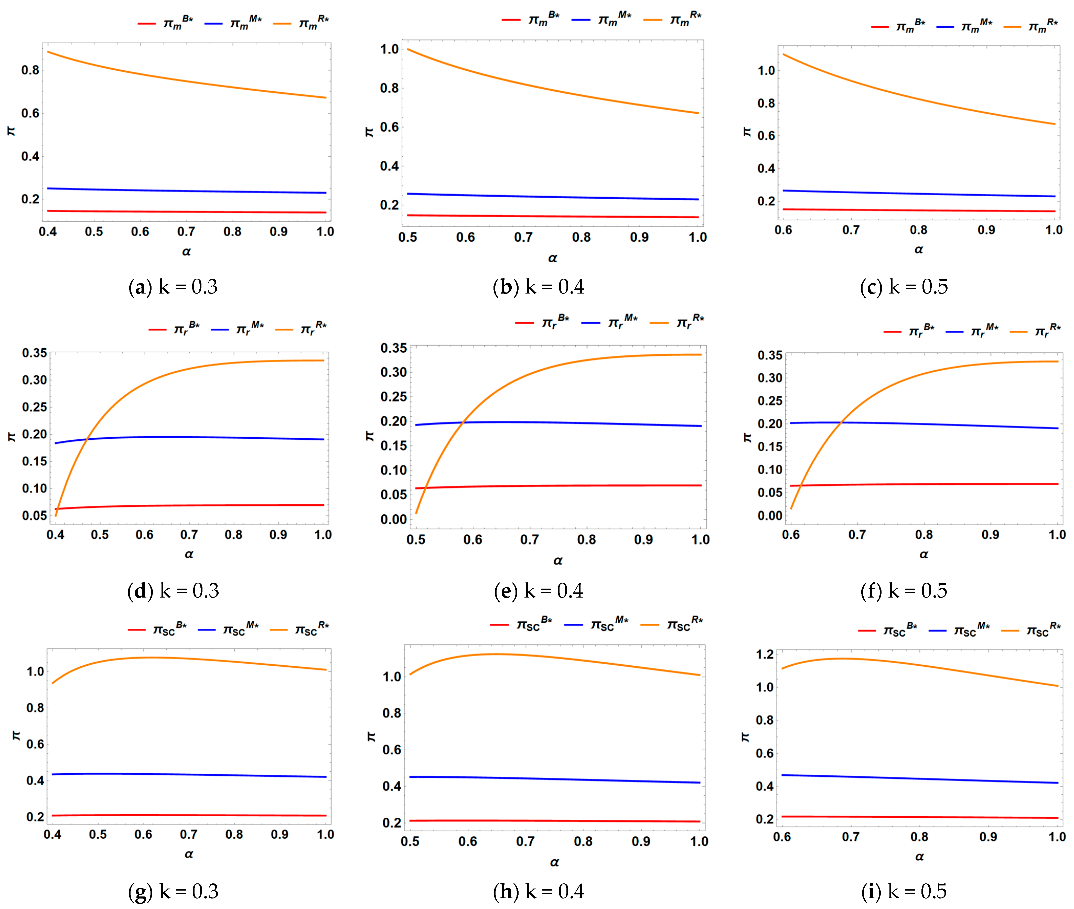
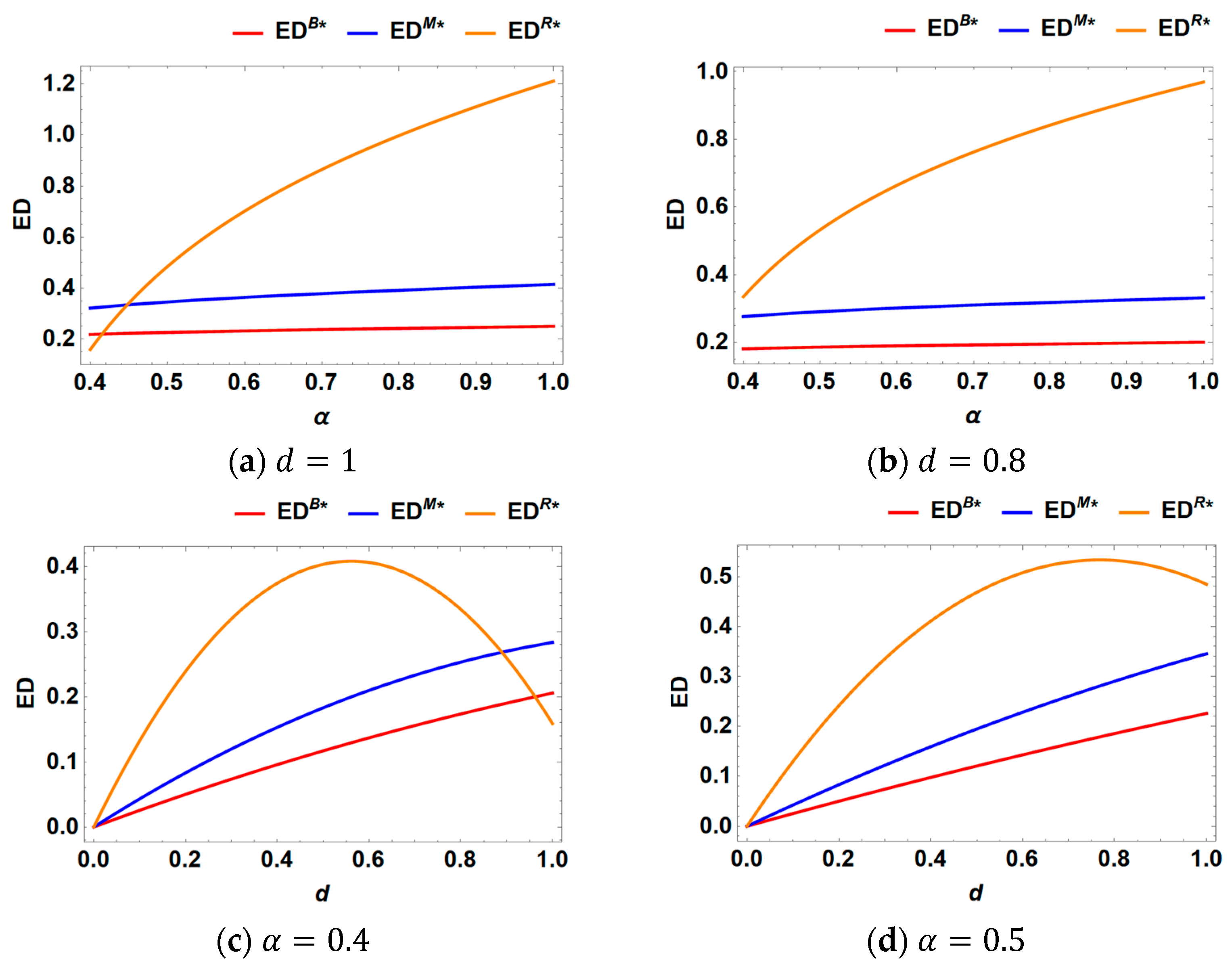
6.1. Profits of Supply Chain and Environmental Damage

Figure 1 depicts the changes in the optimal profits of manufacturers, retailers, and the entire supply chain with the intensity of recycling competition under different scenarios. In this example, the parameters are set to c = 0.6 ,   z = 0.7 ,   β = 0.9 ,   and   d = 1 . The cost-saving parameters k from recycled products are set to 0.3, 0.4, and 0.5. For each parameter system, we constrained the value of parameter α to guarantee the existence of an optimal solution and to ensure the non-negativity of the resulting solution.
By comparing the three curves in Figure 1a–c, we can observe that the manufacturer always prefers the retailer, who is closer to the market and has pricing power, to undertake advertising efforts. In contrast, a comparison of the three curves in Figure 1d–f reveals that when recycling competition intensity is low, the retailer prefers the manufacturer to carry out advertising efforts. However, when competition intensity is relatively high, the retailer prefers to conduct market promotions themselves. This suggests that under high recycling competition intensity, the strategic preferences of the manufacturer and retailer can align. By comparing g–i in Figure 1, it is evident that when retailers engage in marketing activities, it yields the greatest benefit to the entire supply chain, significantly outperforming the other two models.
Next, we examine the impact of recycling competition intensity on both supply chain members and overall supply chain performance when retailers engage in marketing (Model R). As shown in Figure 1a–c, the manufacturer’s profit ( π m R ) consistently decreases with increasing competitive intensity in recycling. This heightened competition raises recycling costs, making it more challenging for the manufacturer to achieve cost savings in remanufacturing. However, Figure 1d–f indicate that the retailer’s optimal profit ( π r R ) tends to increase as the competitive intensity of recycling rises. This upward trend becomes particularly pronounced under conditions of relatively low competitive intensity. This increase in profit can be attributed to two factors: a decrease in wholesale prices driven by higher competition intensity and a reduction in recycling costs resulting from lower recycling intensity.
From Figure 1g–i, when the retailer exerts marketing efforts, it is evident that the profit of the entire supply chain ( π S C R ) increases as the intensity of recycling competition grows when the competition intensity is low. As the intensity of recycling competition increases, it reduces the incentive for supply chain members to engage in recycling, thereby diminishing production cost savings. In contrast, increased competition intensity reduces the retailer’s incentive to recycle and their willingness for wholesale. Thus, the supplier is motivated to lower the wholesale price to encourage the retailer’s wholesaling. This, in turn, mitigates the double marginalization effect and enhances the profitability of the entire supply chain. The interaction of these two forces reveals that as the intensity of competition increases, the profitability of the entire supply chain initially rises and then falls. Therefore, when the competition intensity is moderate, the effect of mitigating the double marginalization effect outweighs the negative impact of reduced recycling incentives.
The variation in environmental damage with the intensity of recycling competition under Models B, M, and R is illustrated in Figure 2a,b. In this example, the parameters are set to k = 0.3 ,   c = 0.6 ,   z = 0.7 ,   β = 0.9 . As shown in Figure 2a,b, it is intuitive that as the intensity of recycling competition increases, environmental damage also rises. This is because higher recycling competition intensity tends to result in reduced recycling efforts. However, environmental damage under Model R is more sensitive to changes in competition intensity. As a result, as shown in Figure 1a, when recycling competition intensity is very low, even though production volume under Model R is high, the recycling rate remains very high, which leads to the lowest environmental damage.
By examining Figure 2c,d, we can observe that under Model R, as the basic demand d increases, environmental damage initially rises. This is due to the fact that higher commodity production leads to greater environmental damage. However, as demand continues to grow, increased sales boost the recycling efforts of both manufacturers and retailers, leading to a higher recycling rate and, ultimately, a reduction in environmental damage. Comparing Figure 2c,d, we find that when the recycling competition intensity is sufficiently low and the basic demand is sufficiently high, the environmental damage under Model R is even lower than that of the other two models.

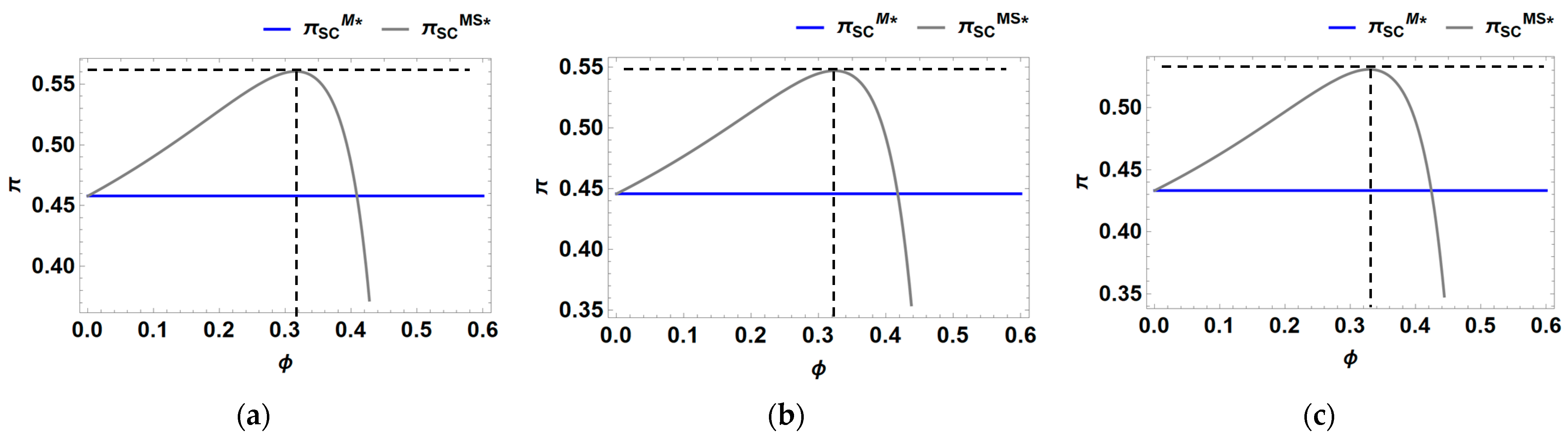
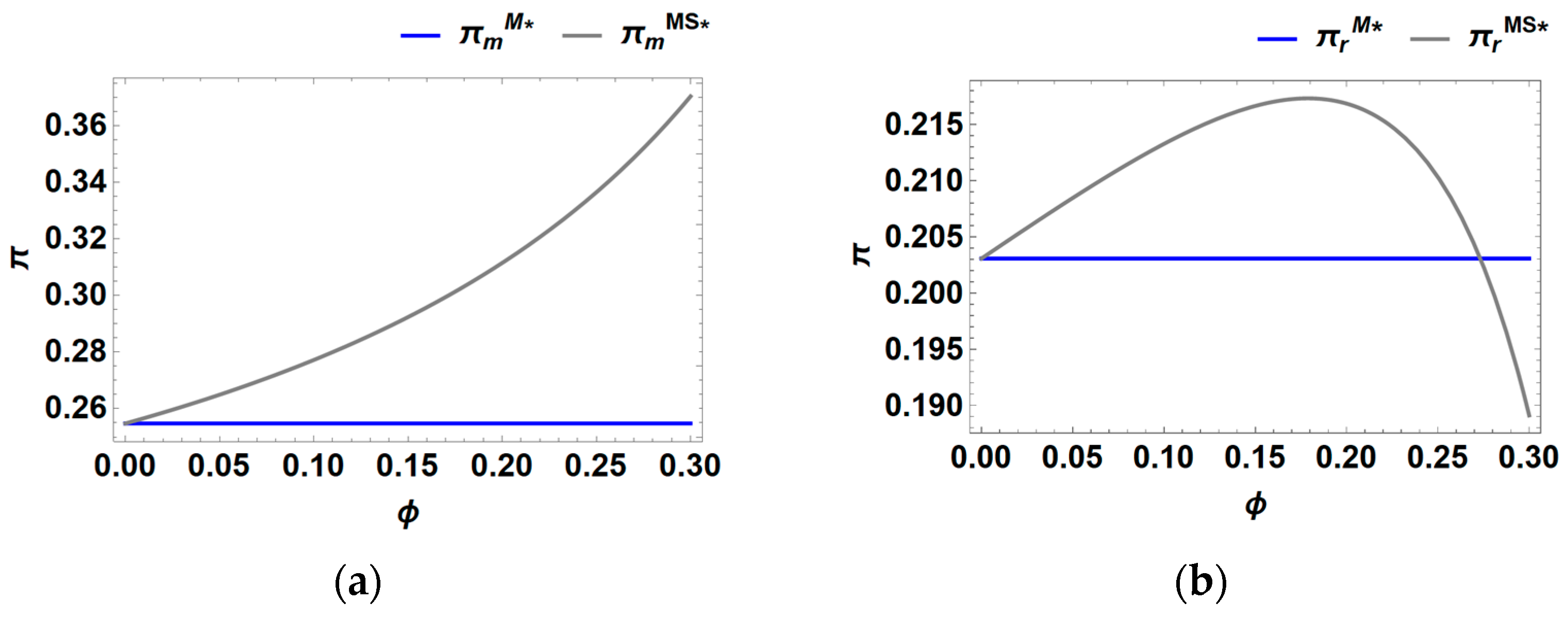
6.2. Marketing Cost Sharing

Marketing cost-sharing contracts are commonly employed in real-world business practices [67,68]. In this section, we examine a supply chain scenario where one party undertakes promotional efforts while the other party proposes a cost-sharing contract, and we analyze its impact on overall supply chain performance. We introduce an exogenous parameter, ϕ , to represent the cost-sharing ratio.

6.2.1. Under Model M

In this subsection, we analyze the retailer’s share of the marketing costs when the manufacturer undertakes marketing efforts. Consequently, the manufacturer’s profit function can be expressed as follows:
D M S = d β   p M S + y M S ,
π m M S = w M S + k   ζ m M S + ζ r M S b M S   ζ r M S   D M S c ζ m M S 2 + α   ζ r M S 2 1 α 2 1 2   ( 1 ϕ )   z   y M S 2 ,
π r M S = p M S + b M S   ζ r M S   D M S c ζ r M S 2 + α   ζ m M S 2 1 α 2 1 2   ϕ   z   y M S 2 .
Figure 3 below illustrates the variation in overall supply chain profit with respect to the cost-sharing proportion ϕ across two scenarios: the manufacturer undertaking marketing efforts (Model M) and the retailer sharing the cost of the manufacturer’s marketing efforts (Model MS).
In Figure 3 above, we can observe that when the manufacturer engages in marketing promotions, there is always an optimal cost-sharing ratio that enhances the profitability of the entire supply chain. Moreover, this optimal ratio increases as the intensity of recycling competition grows. Next, we examined whether the retailer is willing to bear this cost-sharing arrangement and whether the manufacturer is inclined to accept it under natural conditions. Using α = 0.7, we illustrated the variation in (a) the manufacturer’s profit and (b) the retailer’s profit with respect to the cost-sharing ratio, considering scenarios where the manufacturer conducts promotions and the retailer participates in cost sharing.
Figure 4 indicates that the retailer is willing to share the manufacturer’s marketing costs at a rate lower than a certain value of ϕ , and the manufacturer is consistently willing to accept this cost sharing. This finding demonstrates that cost sharing by the retailer, when the manufacturer conducts promotions, can enhance profitability for both parties.

6.2.2. Under Model R

In this subsection, we analyze the manufacturer’s share of the marketing costs when the retailer undertakes marketing efforts. Consequently, the manufacturer’s profit function can be expressed as follows:
D R S = d β   p R S + y R S ,
π m R S = w R S + k   ζ m R S + ζ r R S b R S   ζ r R S   D R S c ζ m R S 2 + α   ζ r R S 2 1 α 2 1 2   ϕ   z   y R S 2 ,
π r R S = p R S + b R S   ζ r R S   D R S 1 2   ( 1 ϕ )   z   y R S 2 .
Figure 5 illustrates the variation in overall supply chain profit with respect to the cost-sharing proportion across three scenarios: the retailer undertaking marketing efforts (Model R), the centralized supply chain engaging in marketing efforts (Model C), and the manufacturer sharing the cost of the retailer’s marketing efforts (Model RS).
In Figure 5, we can observe that for the entire supply chain, an optimal cost-sharing ratio always exists that enhances the supply chain’s performance compared to the scenario without cost sharing. However, this performance remains lower than that of a centralized supply chain. Additionally, the optimal subsidy ratio increases as the intensity of recycling competition rises.
Next, we analyzed whether, under natural conditions, the manufacturer is willing to share the retailer’s costs and whether the retailer is inclined to accept the manufacturer’s cost-sharing proposal. The following figures illustrate (a) the manufacturer’s profit and (b) the retailer’s optimal profit under Models R and RS, respectively, when α = 0.7.
Figure 6 reveals an interesting dynamic: while the manufacturer shows a willingness to engage in marketing cost sharing with the retailer, the retailer is reluctant to accept such an arrangement. This reluctance stems from the fact that when the manufacturer shares the marketing costs, it gains greater influence over the retailer’s marketing decisions. Moreover, as the supplier holds a first-mover advantage, it can leverage this position to increase its own profits by raising the wholesale price, ultimately reducing the retailer’s profitability. Consequently, under natural circumstances, cooperation involving the manufacturer sharing the retailer’s marketing costs is unlikely to occur unless the manufacturer is compensated with an additional fixed payment.

6.3. Consider the Production Cost

In the theoretical framework established in Section 3, we adopt the simplifying assumption of zero-unit production cost to maintain model brevity. However, recognizing that actual production processes inevitably incur substantial costs across multiple dimensions, this subsection extends the analysis to incorporate production costs c m , thereby enhancing the model’s practical relevance and analytical robustness. Specifically, we revise the manufacturer’s profit function to account for these production costs, with the modified formulation presented in Table 2. The parameters in the latter figure take the values of k = 0.3 ,   c = 0.6 , z = 0.7 , β = 0.9 , d = 1 .
Figure 7 presents the profits of supply chain members and the overall supply chain under different production cost scenarios ( c m = 0.1 and 0.2 ). The comparative analysis reveals that while increased production costs negatively affect the profitability of both individual supply chain members and the collective supply chain system, these cost variations do not fundamentally alter our primary theoretical conclusions. This finding demonstrates the robustness of our main findings across different production cost structures.

6.4. Consider the Government Subsidy

In this section, we examine the scenario in which the government provides a subsidy to incentivize manufacturers’ remanufacturing activities. Specifically, we consider a government subsidy scheme where the manufacturer receives a subsidy of GS per unit of remanufactured product produced. This subsidy mechanism aims to promote sustainable manufacturing practices and encourage the development of circular economy initiatives within the manufacturing sector. In the subsidized scenario, the manufacturer’s profit function under the three models can be rewritten as follows in Table 3. The parameters in the latter figure take the values of k = 0.3 ,   c = 0.6 , z = 0.7 , β = 0.9 , d = 1 , G S = 0.1 .
As illustrated in Figure 8, the government subsidy exerts a direct impact on the manufacturer’s remanufacturing operations, resulting in a consistent enhancement of the manufacturer’s profitability across all three marketing models. This positive effect is particularly pronounced under conditions of lower recycling competition intensity, where the manufacturer can capitalize more effectively on the subsidy to optimize its remanufacturing processes and maximize profit margins.
As illustrated in Figure 9, a government subsidy for the manufacturer’s remanufacturing initiatives may inadvertently lead to a reduction in the retailer’s profit. This counterintuitive outcome stems from the dual-channel impact of such a subsidy: while it incentivizes manufacturers to raise the recycling price in the reverse supply chain, it simultaneously encourages manufacturers to increase wholesale prices in the forward supply chain. Under conditions of relatively low market competition intensity, where retailers possess limited competitive advantage in the recycling market, the adverse effects of elevated wholesale prices in the forward channel become predominant. Consequently, the net impact manifests as a deterioration in retailers’ profitability, as the cost escalation in the forward channel outweighs the potential benefits from the reverse channel operations.
As shown in Figure 10, in terms of overall supply chain profitability, a government subsidy has the most pronounced uplift effect on the supply chain when the intensity of recycling competition is moderate. When the intensity of competition is low, a government subsidy can even harm supply chain profits, as retailers suffer more from large increases in wholesale prices.

7. Conclusions

7.1. Theoretical Contributions

Marketing in the forward channel and recycling competition in the reverse channel are integral components of CLSCs and exhibit a dynamic interplay that influences the overall efficiency and effectiveness of the system. Previous studies have predominantly examined marketing in the forward channel and recycling competition in the reverse channel as separate entities. However, in this study, we integrate these two components into a unified framework, providing a holistic perspective on their interdependence and mutual influence. Our study advances the theory of marketing strategy selection for manufacturers and retailers in CLSCs by incorporating an analysis of four distinct marketing models. In addition, this study explores the potential for optimizing supply chains and enhancing the performance of supply chain members through the implementation of marketing cost-sharing contracts. Finally, we analyze the impact of a government subsidy on supply chain performance from the perspective of recycling competition intensity.

7.2. Main Results and Managerial Insights

Our main results are as follows:
(1)
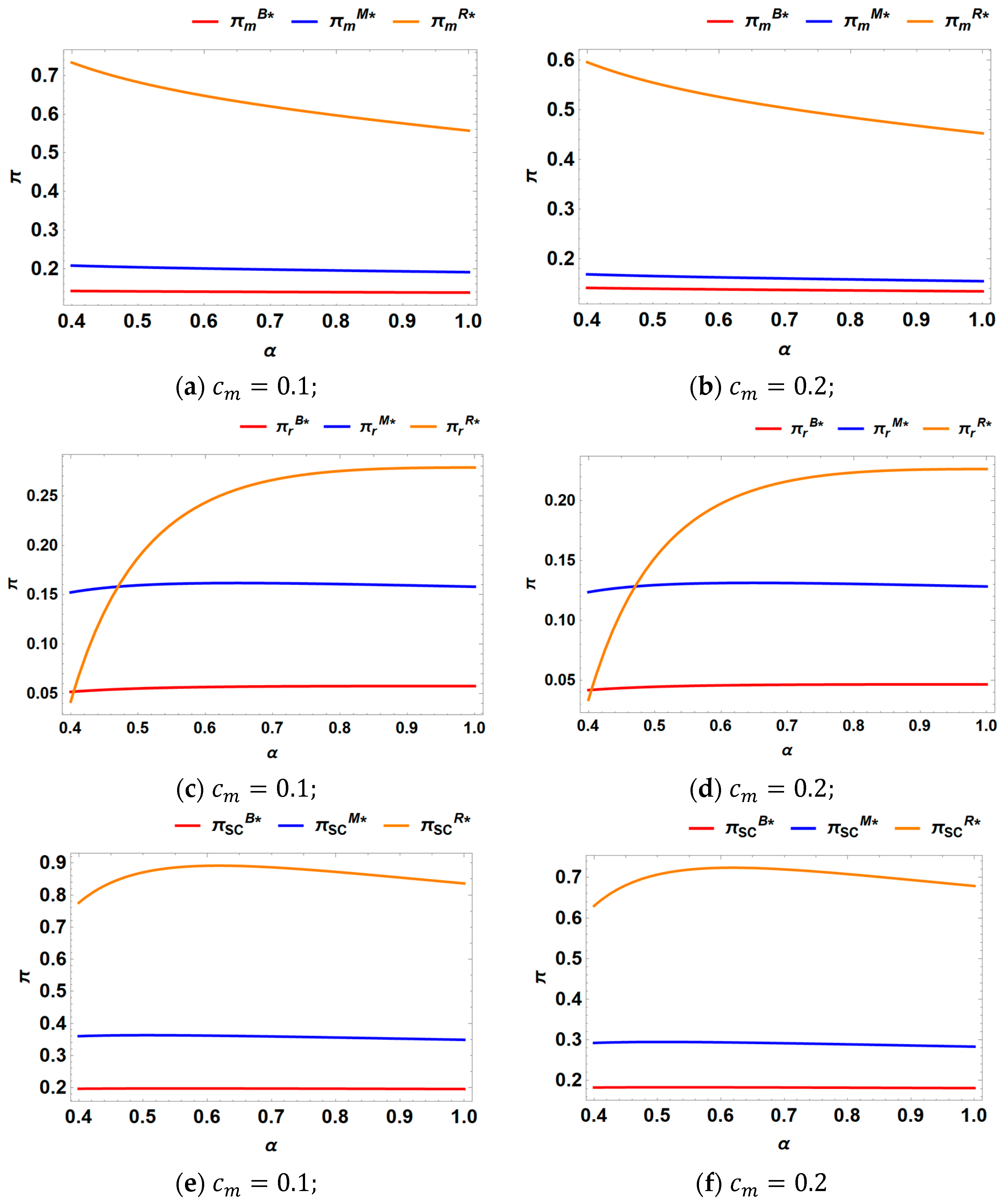
Implementing marketing measures consistently leads to higher profits for the manufacturer, retailer, and overall supply chain compared to scenarios where no marketing efforts are undertaken. However, the manufacturer consistently prefers the retailer to undertake marketing efforts. In contrast, the retailer’s strategic preference varies based on the intensity of recycling competition. Specifically, the retailer prefers the manufacturer to handle marketing when the competition intensity is low, whereas they opt to undertake their own marketing efforts when the competition intensity is high.
(2)
Retailer-led marketing leads to higher prices, greater marketing efforts, increased demand, enhanced recycling efforts, and lower wholesale prices compared to manufacturer-led marketing. However, the buyback prices of recycled materials remain unaffected by which party undertakes the marketing. In addition, the environmental impact of different models is influenced by the underlying demand. As the base demand increases, the order of models with the lowest environmental damage shifts progressively: no marketing, marketing by manufacturers, and marketing by retailers.
(3)
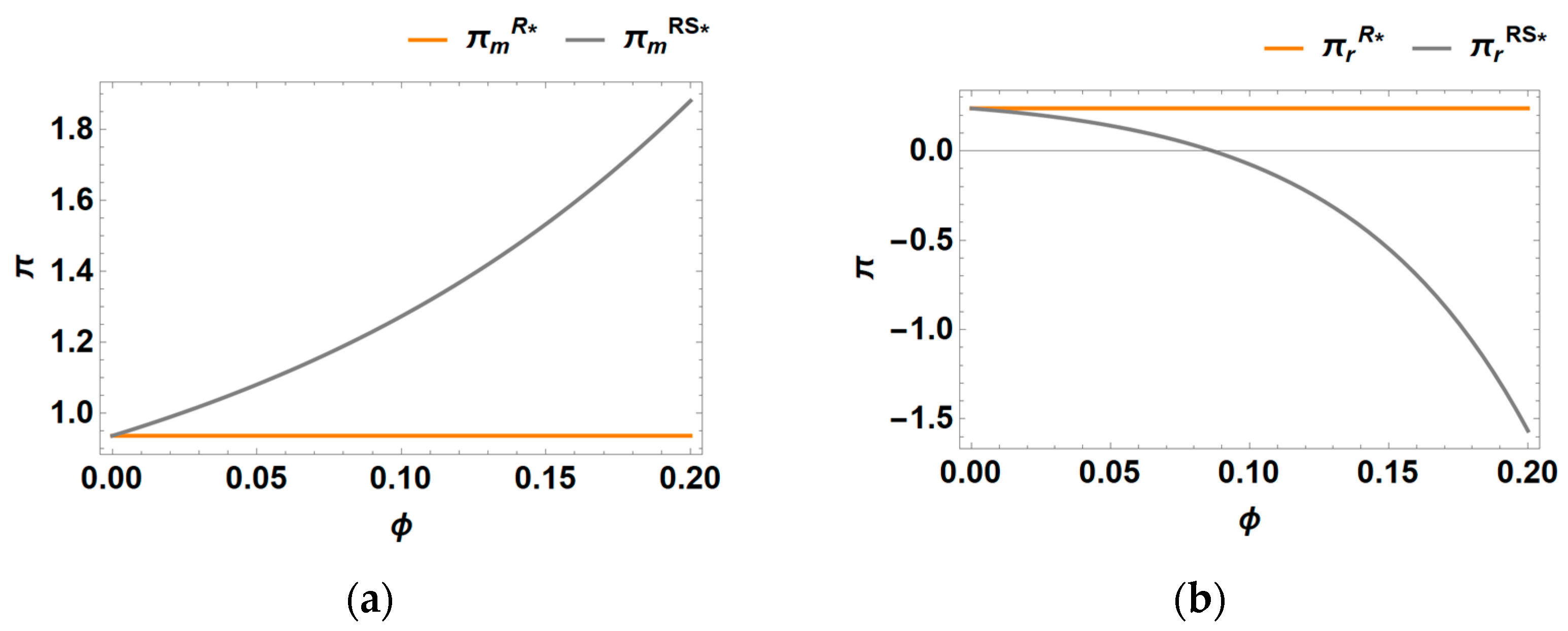
Higher competitive intensity in recycling results in reduced recycling efforts, lower buyback prices, decreased wholesale prices, and diminished marketing efforts. However, in the absence of marketing, prices increase as recycling competition intensity rises. Conversely, when marketing is present, prices decrease as recycling competition intensity increases. As the intensity of competition rises, manufacturers’ margins always fall, while retailers’ margins tend to rise, and the margins of the entire supply chain rise and then fall. The impact of recycling competition intensity on environmental damage depends on the base demand: it decreases with higher competition intensity when the base demand is low but increases when the base demand is high.
(4)
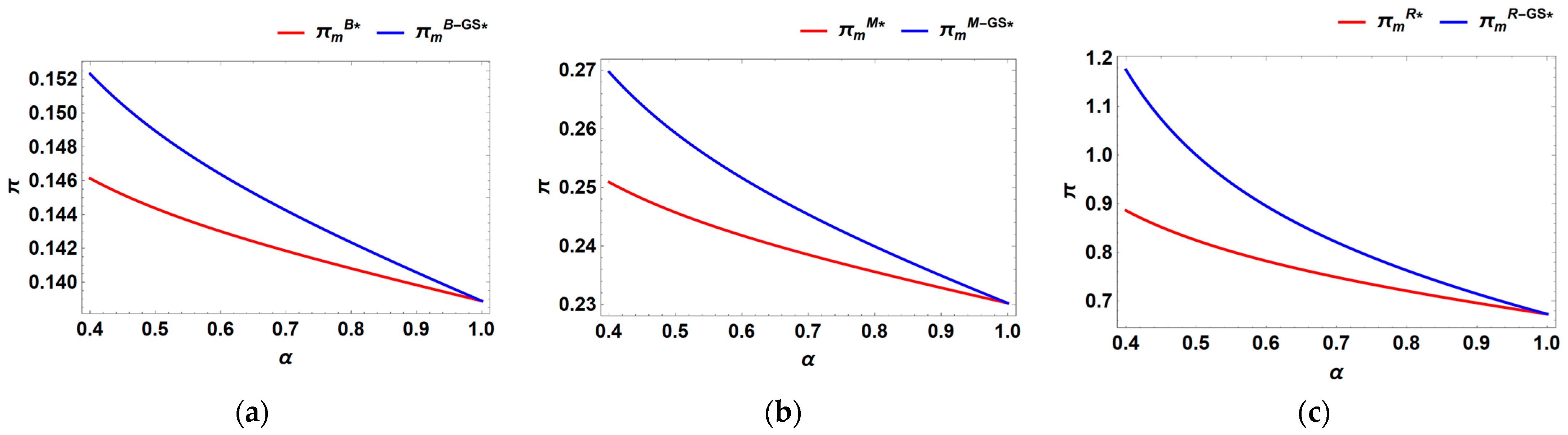
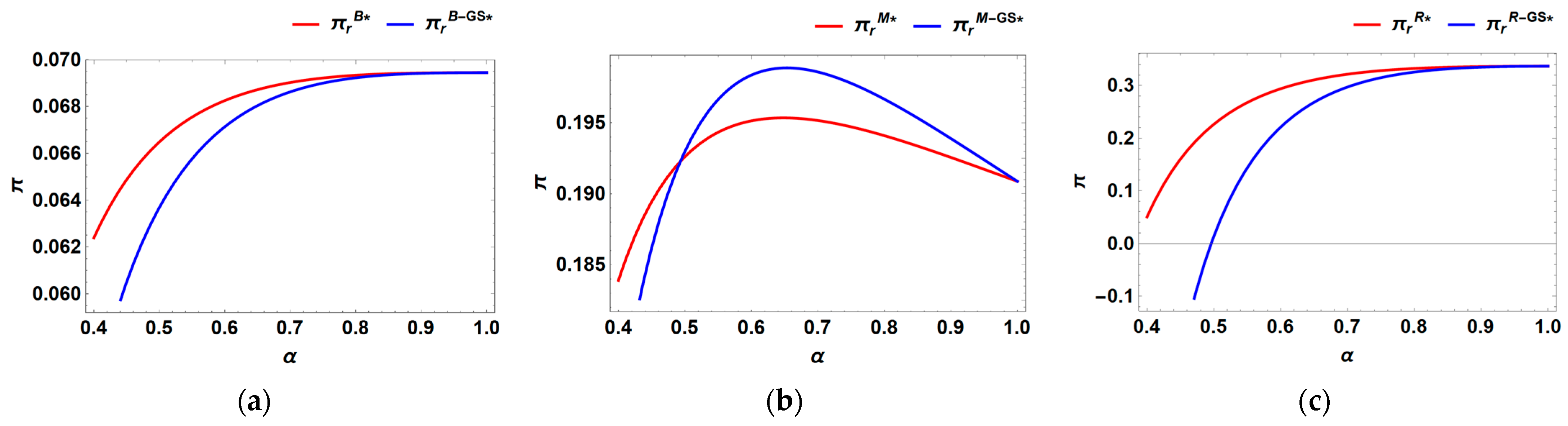
There is always an optimal marketing cost-sharing ratio that enhances supply chain profits. When the manufacturer undertakes marketing, cost sharing improves the profits of both the retailer and the manufacturer. However, when the retailer handles marketing, cost sharing reduces the retailer’s profits, necessitating a contract for coordination.
Our results provide the following key managerial insights:
(1)
An optimal level of recycling competition, rather than an excessively high or low intensity, enhances the profitability of the entire supply chain by strengthening the retailer’s position in recycling and balancing the power dynamics between the manufacturer and retailer. Moreover, at this appropriate level of competition, manufacturers and retailers are more likely to align their marketing strategies, such as delegating marketing responsibilities to retailers. Therefore, supply chain members can intensify recycling promotion efforts to maintain recycling competition within an optimal range, thereby facilitating the coordination of marketing strategies and boosting the profits of supply chain members.
(2)
Supply chain members can further optimize profits by sharing marketing costs and establishing contracts. This approach remains effective even in the context of recycling competition.
(3)
From an environmental protection standpoint, a larger demand base can lead to increased recycling efforts and reduced environmental harm. Consequently, government and relevant environmental agencies can enhance recycling rates by encouraging the integration of smaller enterprises with larger ones, thereby fostering collective environmental responsibility. This approach helps optimize resources, reduce waste, and protect the environment more effectively.
(4)
A government subsidy to the manufacturer invariably enhances its profitability. However, when recycling competition is weak, such a subsidy can significantly harm the retailer’s profitability and consequently disrupt the entire supply chain. The government should implement a subsidy when recycling competition is at a moderate level, as this can lead to greater overall profitability across the supply chain.

7.3. Limitations and Future Studies

This study has the following limitations: First, this study assumes that consumers value new and remanufactured products equally, which is valid in certain industries. However, in many other industries, remanufactured products are perceived as less valuable than new ones, suggesting that further research into valuation disparities is warranted. Second, the description of environmental damage in this article is too simple. It would be more reasonable to evaluate the environmental impact of closed-loop supply chains through life-cycle assessment methods. Third, it focuses on a single supply chain in the forward channel, while the increasing prevalence of manufacturers with their own direct marketing channels could be explored in future research. Finally, the demand in this study is assumed to be fixed, leaving room for further investigation into marketing strategies under uncertain demand conditions.

Author Contributions

Conceptualization, X.T., L.W. and Z.L.; methodology, X.T., Z.L. and L.W.; software, X.T. and L.W.; writing—original draft preparation, X.T. and Z.L.; writing—review and editing, X.T. and L.W. All authors have read and agreed to the published version of the manuscript.

Funding

This work is supported by the Research Projects of Universities in Anhui Province (2024AH050001).

Institutional Review Board Statement

Not applicable.

Informed Consent Statement

Not applicable.

Data Availability Statement

No new data were created or analyzed in this study.

Acknowledgments

The authors would like to thank the editors and the anonymous review team for their highly constructive comments on earlier versions of this article. The authors are grateful to Jiahui Wu for her help with the case collection and case calculations.

Conflicts of Interest

The authors declare no conflicts of interest.

Appendix A

Proof of Proposition 1. 
The first-order derivatives of π r B to p B and ζ r B can be shown as follows:
π r B p B = d + β   ( 2   p B + w b   ζ r B ) ,
π r B ζ r B = b B ( d p p β ) + 2 c ζ r 1 + α 2 .
The Hessian matrix of π r B is the following:
R B = 2 β b B β b B β 2 c 1 α 2
since R B 1 = 2 β < 0 , R B = 4 c β 1 α 2 b B 2 β 2 . To ensure that π r B is jointly concave with respect to p B and ζ r B , we assume b B < 4 c β β ( 1 α 2 ) . Further, by solving π r B p B = 0 and π r B ζ r B = 0 , we can obtain the following:
p B ( b B , w B ) = b B 2 d ( 1 + α 2 ) β + 2 c ( d + w B β ) β ( 4 c + b B 2 ( 1 + α 2 ) β ) ,
ζ r B ( b B , w B ) = b B ( 1 + α 2 ) ( d w B β ) 4 c + b B 2 ( 1 + α 2 ) β .
Then, by substituting (A4) and (A5) into Equation (5) and taking the first-order derivatives of π m B to ζ m B and w B , we obtain the following:
π m B ζ m B = 2 c ( k ( d w B β ) 4 c + b B 2 ( 1 + α 2 ) β + ζ m B 1 + α 2 ) ,
π m B w B = 2 c ( c ( 4 d + 8 w B β + 4 k β ζ m B ) + b B ( 1 + α 2 ) β ( 2 k ( d w B β ) + b B ( d + d α w B α β + k β ζ m B ) ) ) ( 4 c + b B 2 ( 1 + α 2 ) β ) 2 .
The Hessian matrix of π m B is the following:
M B = 2 c 1 + α 2 2 c k β 4 c + b B 2 ( 1 + α 2 ) β 2 c k β 4 c + b B 2 ( 1 + α 2 ) β 2 c β ( 8 c + b B ( 2 k b B α ) ( 1 + α 2 ) β ) ( 4 c + b B 2 ( 1 + α 2 ) β ) 2 ,
M B 1 = 2 c 1 α 2 < 0 , and we assume M B = 4 c 2 β ( 8 c + ( 2 b B k k 2 + b B 2 α ) ( 1 + α 2 ) β ) ( 1 + α 2 ) ( 4 c + b B 2 ( 1 + α 2 ) β ) 2 > 0 to ensure that π m B is jointly concave with respect to w B and ζ m B . By solving π m B ζ m B = 0 and π m B w B = 0 , we obtain the following:
ζ m B ( b B ) = d k ( 1 + α 2 ) 8 c ( 2 b B k k 2 + b m 2 α ) ( 1 + α 2 ) β ,
w B ( b B ) = d ( 4 c + ( 1 + α 2 ) ( 2 b B k k 2 + b B 2 ( 1 + α ) ) β ) β ( 8 c + ( 2 b B k k 2 + b B 2 α ) ( 1 + α 2 ) β ) .
By substituting (A9) and (A10) into Equation (5), we obtain the following:
π m B b B = c d 2 β ( 8 c + ( 2 b B k k 2 + b B 2 α ) ( 1 + α 2 ) β ) ,
Then, we find that π m B b B increases when b B increases between ( 0 , k α ) and decreases when b B increases over k α . Then, we obtain the optimal recycling price: b B = k α .
Substituting Equation b B = k α into relative functions, we can obtain the optimal wholesale price, recycling efforts, sales price, and profits.
The optimal decisions can be substituted into the following:
C S B = ( d β p B ) 2 2 ,
E D M = θ ( 1 ζ m B ζ r B ) ( d β p B )
Then, we can obtain the optimal consumer surplus and environmental damage as follows:
C S M = 2 c 2 d 2 α 2 ( 8 c α + k 2 ( 1 + α ) ( 1 + α ) 2 β ) 2 ,
E D M = 2 c d α ( 8 c α + d k ( 1 + α ) ( 1 + α ) 2 + k 2 ( 1 + α ) ( 1 + α ) 2 β ) θ ( 8 c α + k 2 ( 1 + α ) ( 1 + α ) 2 β ) 2 .
In order for the concave conditions of π m B and π r B and the non-negative demand function to be satisfied, we need the conditions below.
k 2 4 + k 2 < α < 1 & k 2 k 2 α 2 4 α 2 < c < 1 & 0 < β < 4 c α 2 k 2 + k 2 α 2 k 2 α 3 + k 2 α 5 .
The proof of Proposition 1 is completed. □
Proof of Proposition 2. 
The first-order derivatives of π r M to p M and ζ r M can be shown as follows:
π r M p M = d + y M + β ( 2 p M + w M b ζ r M ) ,
π r M ζ r M = b d + y M p M β 2   c   ζ r M 1 α 2 .
The Hessian matrix of π r M is the following:
R M = 2 β b M β b M β 2 c 1 α 2
since R M 1 = 2 β < 0 , R M = 4 c β 1 α 2 b M 2 β 2 . To ensure that π r M is jointly concave with respect to p M and ζ r M , we assume b M < 4 c β β ( 1 α 2 ) . Further, by solving π r M p M = 0 and π r M ζ r M = 0 , we can obtain the following:
p M ( b M , w M , y M ) = b 2 d + y M 1 α 2 β 2 c ( d + y M + w M β ) β ( 4 c b M 2 ( 1 α 2 ) β ) ,
ζ r M ( b M , w M , y M ) = b M ( 1 + α 2 ) ( d + y M w M β ) 4 c b M 2 ( 1 α 2 ) β .
Then, by substituting (A20) and (A21) into Equation (19) and taking the first-order derivatives of π m M to ζ m M , w M and y M , we obtain the following:
π m M ζ m M = 2 c ( k d y M + w M β 4 c b B 2 1 α 2 β ζ m M 1 α 2 ) ,
π m M w M = 2 c ( 4 c d + y M β 2 w M + k ζ m M + b M ( 1 α 2 ) β ( 2 k ( d + y M w M β ) + b M ( d + y M + d α + y M α w M α β + k β ζ m M ) ) ) ( 4 c b M 2 ( 1 α 2 ) β ) 2 ,
π m M y B = b 4 y M z 1 + α 2 2 β 2 4 b c k ( 1 + α 2 ) ( d + y M w M β ) + 8 c 2 ( w M 2 y M z + k ζ m M ) + 2 b 2 c ( 1 + α 2 ) ( d ( 2 + α ) + y M ( 2 + α 4 z β ) β ( w M + w M α k ζ m M ) ) ( 4 c + b M 2 ( 1 + α 2 ) β ) 2 ,
The Hessian matrix of π m M is as follows:
M M = 2 c β ( 8 c + b M ( 2 k b M α ) ( 1 + α 2 ) β ) ( 4 c b 2 ( 1 α 2 ) β ) 2 2 c k β 4 c b M 2 ( 1 α 2 ) β 2 c ( 4 c + b M ( b M 2 k + b M α ) ( 1 α 2 ) β ) ( 4 c b M 2 ( 1 α 2 ) β ) 2 2 c k β 4 c b M 2 ( 1 α 2 ) β 2 c 1 α 2 2 c k 4 c b M 2 ( 1 α 2 ) β 2 c ( 4 c + b M ( b M 2 k + b M α ) ( 1 α 2 ) β ) ( 4 c b M 2 ( 1 α 2 ) β ) 2 2 c k 4 c b M 2 ( 1 α 2 ) β 16 c 2 z 4 b M c k 1 α 2 + b M 4 z 1 α 2 2 β 2 + 2 b M 2 c ( 1 α 2 ) ( 2 + α 4 z β ) ( 4 c b M 2 ( 1 α 2 ) β ) 2 ,
We assume M M 1 = 2 c 1 α 2 < 0 , M M 2 = 4 c 2 β ( 8 c + ( 2 b M k k 2 + b M 2 α ) ( 1 + α 2 ) β ) ( 1 + α 2 ) ( 4 c + b M 2 ( 1 + α 2 ) β ) 2 > 0 M M = 4 c 2 z 2 b M k k 2 + b M 2 α 1 + α 2 β 2 + c 2 8 z β 1 + α 2 4 c + b M 2 1 + α 2 β 2 < 0 to ensure that π m B is jointly concave with respect to w M , ζ m M and y M . By solving π m B ζ m B = 0 , π m B w B = 0 , and π m B y B = 0 , we obtain the following:
ζ m M ( b M ) = d k z ( 1 α 2 ) β z ( 2 b M k k 2 + b M 2 α ) ( 1 + α 2 ) β 2 + c ( 2 + 8 z β ) ,
w M b M = d z 4 c 1 + α 2 2 b M k k 2 + b M 2 1 + α β z 2 b M k k 2 + b M 2 α 1 + α 2 β 2 + c 2 + 8 z β ,
y M b M = 2 c d z ( 2 b M k k 2 + b M 2 α ) ( 1 + α 2 ) β 2 + c ( 2 8 z β ) .
Substituting (A26), (A27), and (A28) into Equation (19), we obtain the following:
π m B b M = c d 2 z z ( 2 b M k k 2 + b M 2 α ) ( 1 + α 2 ) β 2 + c ( 2 8 z β ) ,
Then, we find that π m B b B increases when b M increases between ( 0 , k α ) and decreases when b M increases over k α . Then, we obtain the optimal recycling price as follows: b M = k α .
Substituting Equation b M = k α into relative functions, we can obtain the optimal wholesale price, recycling efforts, marketing efforts, sales price, and profits.
The optimal decisions can be substituted into the following:
C S M = ( d β p M + y M ) 2 2 ,
E D M = θ ( 1 ζ m M ζ r M ) ( d β p M + y M ) .
Then, we can obtain the optimal consumer surplus and environmental damage as follows:
C S M = 2 c 2 d 2 z 2 α 2 β 2 ( k 2 z ( 1 + α ) ( 1 + α ) 2 β 2 + 2 c α ( 1 + 4 z β ) ) 2 ,
E D M = 2 c d z α β ( k z ( 1 + α ) ( 1 + α ) 2 β ( d + k β ) + 2 c α ( 1 + 4 z β ) ) θ ( k 2 z ( 1 + α ) ( 1 + α ) 2 β 2 + 2 c α ( 1 + 4 z β ) ) 2 .
In order for the concave conditions of π m M and π r M and the non-negative demand function to be satisfied, we need the conditions below:
k 2 4 + k 2 < α < 1 & k 2 k 2 α 2 4 α 2 < c < 1 & 0 < β < 4 c α 2 k 2 + k 2 α 2 k 2 α 3 + k 2 α 5 & z > 2 c α 8 c α β k 2 β 2 k 2 α β 2 + k 2 α 2 β 2 + k 2 α 3 β 2 .
The proof of Proposition 2 is completed. □
Proof of Proposition 3. 
The first-order derivatives of π r R to p R , ζ r R and y R can be shown as follows:
π r R p R = d + y R + β ( 2 p R + w R b R ζ r R ) ,
π r R ζ r R = b R d + y R p R β 2 c ζ r R 1 α 2 ,
π r R y R = p R w R y R z + b R ζ r R .
The Hessian matrix of π r R is the following:
R R = 2 β b R β 1 b R β 2 c 1 α 2 b R 1 b R z
since R R 1 = 2 β < 0 , R R 2 = β ( 4 c 1 α 2 b R 2 β ) , R R = b R 2 z β 2 + c ( 2 4 z β ) 1 α 2 . To ensure that π r R is jointly concave with respect to p R , ζ r M and y R , we assume b R < 4 c β β ( 1 α 2 ) and b R 2 z β 2 + c ( 2 4 z β ) 1 α 2 < 0 . Further, by solving π r R p R = 0 , π r R ζ r R = 0 , and π r R y R = 0 we can obtain the following:
p R ( b R , w R ) = b R 2 d z ( 1 + α 2 ) β + 2 c ( d z + w R ( 1 + z β ) ) b R 2 z ( 1 + α 2 ) β 2 + c ( 2 + 4 z β ) ,
ζ r M ( b M , w M ) = b R z ( 1 + α 2 ) β ( d + w R β ) b R 2 z ( 1 + α 2 ) β 2 + c ( 2 + 4 z β ) ,
y R b R ,   w R = 2 c ( d w R β ) b R 2 z ( 1 + α 2 ) β 2 + c ( 2 + 4 z β ) .
Then, substituting (A39), (A40), and (A41) into Equation (34) and taking the first-order derivatives of π m R to ζ m R and w R , we obtain the following:
π m R ζ m R = 2 c k z β ( d + w R β ) b R 2 z ( 1 + α 2 ) β 2 + c ( 2 + 4 z β ) + 2 c ζ m R 1 + α 2 ,
π m R w R = 2 c z β ( 2 c ( 1 + 2 z β ) ( d β ( 2 w R + k ζ m R ) ) b R z ( 1 + α 2 ) β 2 ( 2 k ( d w R β ) + b R ( d + d α w R α β + k β ζ m R ) ) ) ( b R 2 z ( 1 + α 2 ) β 2 + c ( 2 + 4 z β ) ) 2 ,
The Hessian matrix of π m M is the following:
M R = 2 c z β 2 ( b R z ( 2 k b R α ) ( 1 + α 2 ) β 2 + c ( 4 + 8 z β ) ) ( b R 2 z ( 1 + α 2 ) β 2 + c ( 2 + 4 z β ) ) 2 2 c k z β 2 b R 2 z ( 1 + α 2 ) β 2 + c ( 2 + 4 z β ) 2 c k z β 2 b R 2 z ( 1 + α 2 ) β 2 + c ( 2 + 4 z β ) 2 c 1 + α 2 ,
We assume M R 1 = 2 c z β 2 ( b R z ( 2 k b R α ) ( 1 + α 2 ) β 2 + c ( 4 + 8 z β ) ) ( b R 2 z ( 1 + α 2 ) β 2 + c ( 2 + 4 z β ) ) 2 < 0 , M R = 4 c 2 z β 2 ( z ( 2 b R k k 2 + b R 2 α ) ( 1 + α 2 ) β 2 + c ( 4 8 z β ) ) ( 1 + α 2 ) ( b R 2 z ( 1 + α 2 ) β 2 + c ( 2 + 4 z β ) ) 2 > 0 to ensure that π m R is jointly concave with respect to w R and ζ m R . By solving π m R ζ m R = 0 and π m R w R = 0 , we obtain the following:
ζ m R ( b R ) = d k z ( 1 + α 2 ) β z ( 2 b R k k 2 + b R 2 α ) ( 1 + α 2 ) β 2 + c ( 4 + 8 z β ) ,
w R b R = d ( z ( 1 + α 2 ) ( 2 b R k k 2 + b 2 ( 1 + α ) ) β 2 + c ( 2 4 z β ) ) z ( 2 b R k k 2 + b R 2 α ) ( 1 + α 2 ) β 3 + c β ( 4 8 z β ) .
Substituting (A45) and (A46) into Equation (35), we obtain the following:
π m R b R = c d 2 z z ( 2 b R k k 2 + b R 2 α ) ( 1 + α 2 ) β 2 + c ( 4 8 z β ) ,
Then, we find that π m R b R increases when b R increases between ( 0 , k α ) and decreases when b R increases over k α . Then, we obtain the optimal recycling price: b R = k α .
Substituting Equation b R = k α into relative functions, we can obtain the optimal wholesale price, recycling efforts, marketing efforts, sales price, and profits.
The optimal decisions can be substituted into the following:
C S R = ( d β p R + y R ) 2 2 ,
E D R = θ ( 1 ζ m R ζ r R ) ( d β p R + y R ) .
Then, we can obtain the optimal consumer surplus and environmental damage as follows:
C S M = 2 c 2 d 2 z 2 α 2 β 2 ( k 2 z ( 1 + α ) ( 1 + α ) 2 β 2 + 4 c α ( 1 + 2 z β ) ) 2 ,
E D M = 2 c d z α β ( k z ( 1 + α ) ( 1 + α ) 2 β ( d + k β ) + 4 c α ( 1 + 2 z β ) ) θ ( k 2 z ( 1 + α ) ( 1 + α ) 2 β 2 + 4 c α ( 1 + 2 z β ) ) 2 .
In order for the concave conditions of π m R and π r R and the non-negative demand function to be satisfied, we need the conditions below:
k 2 4 + k 2 < α < 1 & k 2 k 2 α 2 4 α 2 < c < 1 & 0 < β < 4 c α 2 k 2 + k 2 α 2 k 2 α 3 + k 2 α 5 & z > 2 c α 2 4 c α 2 β k 2 β 2 + k 2 α 2 β 2 k 2 α 3 β 2 + k 2 α 5 β 2 .
The proof of Proposition 3 is completed. □
Proof of Proposition 4. 
The first-order derivatives of π S C C to p C , ζ m C , ζ r C and y C can be shown as follows:
π S C C p C = d + y C β ( 2 p C + k ( ζ m C + ζ r C ) ) ,
π S C C ζ m C = d k + k y C p C β 2 c ζ m C 1 α ,
π S C C ζ r C = d k + k y C p C β 2 c ζ r C 1 α ,
π S C C y C = p C y C z + k ( ζ m C + ζ r C ) .
The Hessian matrix of π S C C is the following:
H C = 2 c 1 + α 0 k β k 0 2 c 1 + α k β k k β k β 2 β 1 k k 1 z .
Since H C 1 = 2 c 1 α < 0 , H C 2 = 2 c 1 α 2 > 0 , we assume H C 3 = 4 c β 2 c k 2 1 α β 1 α 2 < 0 , H C 4 = 4 c ( k 2 z ( 1 + α ) β 2 + c ( 1 + 2 z β ) ) ( 1 α ) 2 > 0 to ensure that π S C C is jointly concave with respect to p C , ζ m C , ζ r C , and y C . By solving π S C C p C = 0 , π S C C ζ m C = 0 , π S C C ζ r C = 0 , and π S C C y C = 0 , we can obtain the following:
p C = d z ( c + k 2 ( 1 + α ) β ) k 2 z ( 1 + α ) β 2 + c ( 1 + 2 z β ) ,
ζ m C = d k z ( 1 + α ) β 2 k 2 z ( 1 + α ) β 2 + c ( 2 + 4 z β ) ,
ζ r C = d k z ( 1 + α ) β 2 k 2 z ( 1 + α ) β 2 + c ( 2 + 4 z β ) ,
y C = c d k 2 z ( 1 + α ) β 2 + c ( 1 + 2 z β ) .
Further, substituting Equations (A58)–(A61) into relative functions, we can obtain the optimal profit.
The optimal decisions can be substituted into the following:
C S C = ( d β p C + y C ) 2 2 ,
E D C = θ ( 1 ζ m C ζ r C ) ( d β p C + y C ) .
Then, we can obtain the optimal consumer surplus and environmental damage as follows:
C S C = c 2 d 2 z 2 β 2 2 ( k 2 z ( 1 + α ) β 2 + c ( 1 + 2 z β ) ) 2 ,
E D C = c d z β ( k z ( 1 + α ) β ( d + k β ) + c ( 1 + 2 z β ) ) θ ( k 2 z ( 1 + α ) β 2 + c ( 1 + 2 z β ) ) 2 .
In order for the concave conditions of π S C C and the non-negative demand function to be satisfied, we need the conditions below:
k 2 4 + k 2 < α < 1 & k 2 k 2 α 2 4 α 2 < c < 1 & 0 < β < 4 c α 2 k 2 + k 2 α 2 k 2 α 3 + k 2 α 5 & z > 2 c α 2 4 c α 2 β k 2 β 2 + k 2 α 2 β 2 k 2 α 3 β 2 + k 2 α 5 β 2 .
The proof of Proposition 4 is completed. □
Proof of Corollary 1. 
The comparison of optimal wholesale price and sales price in different models is as follows:
According to the conditions of (A16), (A34), (A52), and (A66), we obtain the following results:
p M p B = 2 c d α 6 c α + k 2 1 + α 1 + α 2 β β 8 c α + k 2 1 + α 1 + α 2 β k 2 z 1 + α 1 + α 2 β 2 + 2 c α 1 + 4 z β > 0 ,
p R p B = 2 c d α 6 c α + k 2 1 + α 1 + α 2 β β 8 c α + k 2 1 + α 1 + α 2 β k 2 z 1 + α 1 + α 2 β 2 + 2 c α 1 + 4 z β > 0 ,
p R p M = 4 c 2 d α 2 1 z β β k 2 z 1 + α 1 + α 2 β 2 + 4 c α 1 + 2 z β k 2 z 1 + α 1 + α 2 β 2 + 2 c α 1 + 4 z β > 0 ,
w M w B = 2 c d 4 c α 2 + k 2 1 α 2 α 2 + α 3 + α 4 β β 8 c α + k 2 1 + α 1 + α 2 β k 2 z 1 + α 1 + α 2 β 2 + 2 c α 1 + 4 z β > 0 ,
w R w B = 2 c d k 2 1 + α 2 2 + 3 α + α 2 8 c α + k 2 1 + α 1 + α 2 β k 2 z 1 + α 1 + α 2 β 2 + 4 c α 1 + 2 z β > 0 ,
w R w M = 2 c d k 2 z 1 + α 2 β 2 + 2 c α 2 1 + 2 z β β k 2 z 1 + α 1 + α 2 β 2 + 4 c α 1 + 2 z β k 2 z 1 + α 1 + α 2 β 2 + 2 c α 1 + 4 z β < 0 .
The proof of Corollary 1 is completed. □
Proof of Corollary 2. 
The comparison of optimal recycling price and recycling efforts in different models is as follows:
According to the conditions of (A16), (A34), (A52), and (A66), we obtain the following results.
It is evident that b B = b M = b R = k α .
ζ m M ζ m B = 2 c d k α 2 ( 1 α 2 ) ( 8 c α + k 2 ( 1 + α ) ( 1 + α ) 2 β ) ( k 2 z ( 1 + α ) ( 1 + α ) 2 β 2 + 2 c α ( 1 + 4 z β ) ) > 0 ,
ζ m R ζ m B = 4 c d k α 2 1 α 2 8 c α + k 2 1 + α 1 + α 2 β k 2 z 1 + α 1 + α 2 β 2 + 4 c α 1 + 2 z β > 0 ,
ζ m R ζ m M = 2 c d k z α 2 1 + α 2 β k 2 z 1 + α 1 + α 2 β 2 + 4 c α 1 + 2 z β k 2 z 1 + α 1 + α 2 β 2 + 2 c α 1 + 4 z β < 0 ,
ζ r M ζ r B = 2 c d k α ( 1 α 2 ) ( 8 c α + k 2 ( 1 + α ) ( 1 + α ) 2 β ) ( k 2 z ( 1 + α ) ( 1 + α ) 2 β 2 + 2 c α ( 1 + 4 z β ) ) > 0 ,
ζ r R ζ r B = 4 c d k α ( 1 α 2 ) ( 8 c α + k 2 ( 1 + α ) ( 1 + α ) 2 β ) ( k 2 z ( 1 + α ) ( 1 + α ) 2 β 2 + 4 c α ( 1 + 2 z β ) ) > 0 ,
ζ r R ζ r M = 2 c d k z α ( 1 α 2 ) β ( k 2 z ( 1 + α ) ( 1 + α ) 2 β 2 + 4 c α ( 1 + 2 z β ) ) ( k 2 z ( 1 + α ) ( 1 + α ) 2 β 2 + 2 c α ( 1 + 4 z β ) ) > 0 .
The proof of Corollary 2 is completed. □
Proof of Corollary 3. 
The comparison of optimal marketing effort and demand in different models is as follows:
According to the conditions of (A16), (A34), (A52), and (A66), we obtain the following results:
y R y M = 4 c 2 d α 2 ( k 2 z ( 1 + α ) ( 1 + α ) 2 β 2 + 4 c α ( 1 + 2 z β ) ) ( k 2 z ( 1 + α ) ( 1 + α ) 2 β 2 + 2 c α ( 1 + 4 z β ) ) > 0 ,
y C y R = c d ( 1 k 2 z ( 1 + α ) β 2 + c ( 1 + 2 z β ) 2 α k 2 z ( 1 + α ) ( 1 + α ) 2 β 2 + 4 c α ( 1 + 2 z β ) ) > 0 .
Therefore, y C > y R > y M .
D M D B = 4 c 2 d α 2 ( 8 c α + k 2 ( 1 + α ) ( 1 + α ) 2 β ) ( k 2 z ( 1 + α ) ( 1 + α ) 2 β 2 + 2 c α ( 1 + 4 z β ) ) > 0 ,
D R D M = 4 c 2 d z α 2 β ( k 2 z ( 1 + α ) ( 1 + α ) 2 β 2 + 4 c α ( 1 + 2 z β ) ) ( k 2 z ( 1 + α ) ( 1 + α ) 2 β 2 + 2 c α ( 1 + 4 z β ) ) > 0 ,
D C D R = c d z β ( 1 k 2 z ( 1 + α ) β 2 + c ( 1 + 2 z β ) 2 α k 2 z ( 1 + α ) ( 1 + α ) 2 β 2 + 4 c α ( 1 + 2 z β ) ) > 0 .
Therefore, D C > D R > D M > D B . The proof of Corollary 3 is completed. □
Proof of Corollary 4. 
The comparison of optimal profits of the manufacturer and supply chain in different models is as follows:
According to the conditions of (A17), (A34), (A52), and (A66), we obtain the following results:
π m M π m B = 2 c 2 d 2 α 2 β ( 8 c α + k 2 ( 1 + α ) ( 1 + α ) 2 β ) ( k 2 z ( 1 + α ) ( 1 + α ) 2 β 2 + 2 c α ( 1 + 4 z β ) ) > 0 ,
π m R π m M = 2 c 2 d 2 z α 2 ( k 2 z ( 1 + α ) ( 1 + α ) 2 β 2 + 4 c α ( 1 + 2 z β ) ) ( k 2 z ( 1 + α ) ( 1 + α ) 2 β 2 + 2 c α ( 1 + 4 z β ) ) > 0 .
Therefore, π m R > π m M > π m B .
π S C M π S C B = c d 2 ( 12 c α 2 + k 2 ( 1 α + α 4 + α 5 ) β β ( 8 c α + k 2 ( 1 + α ) ( 1 + α ) 2 β ) 2 + z ( k 2 z ( 1 α + α 4 + α 5 ) β 2 + 2 c α 2 ( 1 + 6 z β ) ) ( k 2 z ( 1 + α ) ( 1 + α ) 2 β 2 + 2 c α ( 1 + 4 z β ) ) 2 ) > 0 ,
π S C R π S C M = c d 2 z ( k 2 z ( 1 α + α 4 + α 5 ) β 2 + 6 c α 2 ( 1 + 2 z β ) ( k 2 z ( 1 + α ) ( 1 + α ) 2 β 2 + 4 c α ( 1 + 2 z β ) ) 2 k 2 z ( 1 α + α 4 + α 5 ) β 2 + 2 c α 2 ( 1 + 6 z β ) ( k 2 z ( 1 + α ) ( 1 + α ) 2 β 2 + 2 c α ( 1 + 4 z β ) ) 2 ) > 0 ,
π S C C π S C R = c d 2 z ( k 2 z ( 1 α + α 4 + α 5 ) β 2 + 6 c α 2 ( 1 + 2 z β ) ( k 2 z ( 1 + α ) ( 1 + α ) 2 β 2 + 4 c α ( 1 + 2 z β ) ) 2 + 1 2 k 2 z ( 1 + α ) β 2 + c ( 2 + 4 z β ) ) > 0 .
Therefore, π S C C > π S C R > π S C M > π S C B . The proof of Corollary 4 is completed. □
Proof of Corollary 5. 
The comparison of optimal consumer surplus and environment in different models is as follows:
According to the conditions of (A16), (A34), (A52), and (A66), we obtain the following results.
Consumer surplus is half the square of demand in this paper; thus, the size of consumer surplus under different models is the same as the demand relationship in the corollary, i.e., S C R > S C M > S C B .
E D M E D B = 2 c d α ( 8 c α + d k ( 1 + α ) ( 1 + α ) 2 + k 2 ( 1 + α ) ( 1 + α ) 2 β ( 8 c α + k 2 ( 1 + α ) ( 1 + α ) 2 β ) 2 + z β ( k z ( 1 + α ) ( 1 + α ) 2 β ( d + k β ) + 2 c α ( 1 + 4 z β ) ) ( k 2 z ( 1 + α ) ( 1 + α ) 2 β 2 + 2 c α ( 1 + 4 z β ) ) 2 ) θ , and when
d < 8 c α + k 2 1 + α 1 + α 2 β k 2 z 1 + α 1 + α 2 β 2 + 2 c α 1 + 4 z β 2 k 1 + α 1 + α 2 k 2 z 1 + α 1 + α 2 β 2 + c α 1 + 8 z β = d 1 , E D M E D B > 0 ; otherwise E D M E D B < 0 .
E D R E D B = 2 c d α ( 8 c α + d k ( 1 + α ) ( 1 + α ) 2 + k 2 ( 1 + α ) ( 1 + α ) 2 β ( 8 c α + k 2 ( 1 + α ) ( 1 + α ) 2 β ) 2 + z β ( k z ( 1 + α ) ( 1 + α ) 2 β ( d + k β ) + 4 c α ( 1 + 2 z β ) ) ( k 2 z ( 1 + α ) ( 1 + α ) 2 β 2 + 4 c α ( 1 + 2 z β ) ) 2 ) θ , and when
d < 8 c α + k 2 1 + α 1 + α 2 β k 2 z 1 + α 1 + α 2 β 2 + 4 c α 1 + 2 z β 2 k 1 + α 1 + α 2 k 2 z 1 + α 1 + α 2 β 2 + 2 c α 1 + 4 z β = d 2 , D R E D B > 0 ; otherwise E D R E D B < 0 .
E D R E D M = 2 c d z α β ( k z ( 1 + α ) ( 1 + α ) 2 β ( d + k β ) + 4 c α ( 1 + 2 z β ) ( k 2 z ( 1 + α ) ( 1 + α ) 2 β 2 + 4 c α ( 1 + 2 z β ) ) 2 k z ( 1 + α ) ( 1 + α ) 2 β ( d + k β ) + 2 c α ( 1 + 4 z β ) ( k 2 z ( 1 + α ) ( 1 + α ) 2 β 2 + 2 c α ( 1 + 4 z β ) ) 2 ) θ , and when
d < k 4 z 2 1 + α 2 1 + α 4 β 4 + 2 c k 2 z 1 + α α 1 + α 2 β 2 3 + 8 z β + 8 c 2 α 2 1 6 z β + 8 z 2 β 2 2 k z 1 α 1 + α 2 β k 2 z 1 + α 1 + α 2 β 2 + c α 3 + 8 z β = d 3 , E D R E D M > 0 . Otherwise, E D R E D M < 0 .
d 1 < d 2 < d 3 , Therefore, when d < d 1 , E D B < E D M < E D R ; when d 1 < d < d 2 , E D M < E D B < E D R ; when d 2 < d < d 3 , E D M < E D R < E D B ; when d > d 3 , E D R < E D M < E D B . The proof of corollary 5 is completed. □
Proof of Corollary 6. 
The partial derivatives of the relevant variables with respect to the intensity of recycling competition are as follows:
ζ m B α = d k 16 c α 3 + k 2 1 + α 2 2 β 8 c α + k 2 1 + α 1 + α 2 β 2 < 0 ,
ζ m M α = d k z β k 2 z 1 + α 2 2 β 2 + 4 c α 3 1 + 4 z β k 2 z 1 + α 1 + α 2 β 2 + 2 c α 1 + 4 z β 2 < 0 ,
ζ m R α = d k z β k 2 z 1 + α 2 2 β 2 + 8 c α 3 1 + 2 z β k 2 z 1 + α 1 + α 2 β 2 + 4 c α 1 + 2 z β 2 < 0 ,
ζ r B α = d k ( 8 c ( 1 + α 2 ) + k 2 ( 1 + α 2 ) 2 β ) ( 8 c α + k 2 ( 1 + α ) ( 1 + α ) 2 β ) 2 < 0 ,
ζ r M α = d k z β ( k 2 z ( 1 + α 2 ) 2 β 2 2 c ( 1 + α 2 ) ( 1 + 4 z β ) ) ( k 2 z ( 1 + α ) ( 1 + α ) 2 β 2 + 2 c α ( 1 + 4 z β ) ) 2 < 0 ,
ζ r R α = d k z β ( k 2 z ( 1 + α 2 ) 2 β 2 4 c ( 1 + α 2 ) ( 1 + 2 z β ) ) ( k 2 z ( 1 + α ) ( 1 + α ) 2 β 2 + 4 c α ( 1 + 2 z β ) ) 2 < 0 ,
b B α = b M α = b R α = k α 2 < 0 ,
w B α = d k 2 ( 1 + α ) ( 4 c α ( 4 + 3 α + 3 α 2 + 2 α 3 ) + k 2 ( 1 + α ) 2 ( 1 α + 2 α 2 ) β ) α 2 ( 8 c α + k 2 ( 1 + α ) ( 1 + α ) 2 β ) 2 < 0 ,
w M α = d z ( k 4 z ( 1 + 2 α ) ( 1 + α 2 ) 2 β 3 + 2 c k 2 α β ( 2 8 z β + α ( 1 + 2 z β ) + α 3 ( 1 + 2 z β ) + α 4 ( 2 + 4 z β ) ) ) α 2 ( k 2 z ( 1 + α ) ( 1 + α ) 2 β 2 + 2 c α ( 1 + 4 z β ) ) 2 < 0 ,
w M α = d k 2 z ( 1 + α ) β ( k 2 z ( 1 + α ) 2 ( 1 α + 2 α 2 ) β 2 + 2 c α ( 4 + 3 α + 3 α 2 + 2 α 3 ) ( 1 + 2 z β ) ) α 2 ( k 2 z ( 1 + α ) ( 1 + α ) 2 β 2 + 4 c α ( 1 + 2 z β ) ) 2 < 0 ,
p B α = 2 c d k 2 ( 1 + α 2 + 2 α 3 ) ( 8 c α + k 2 ( 1 + α ) ( 1 + α ) 2 β ) 2 > 0 ,
p M α = 2 c d k 2 z ( 1 + α 2 + 2 α 3 ) β ( 1 + z β ) ( k 2 z ( 1 + α ) ( 1 + α ) 2 β 2 + 2 c α ( 1 + 4 z β ) ) 2 < 0 ,
p R α = 2 c d k 2 z ( 1 + α 2 + 2 α 3 ) β ( 1 + z β ) ( k 2 z ( 1 + α ) ( 1 + α ) 2 β 2 + 4 c α ( 1 + 2 z β ) ) 2 ,
y M α = 2 c d k 2 z 1 + α 2 + 2 α 3 β 2 k 2 z 1 + α 1 + α 2 β 2 + 2 c α 1 + 4 z β 2 < 0 ,
y R α = 2 c d k 2 z 1 + α 2 + 2 α 3 β 2 k 2 z 1 + α 1 + α 2 β 2 + 4 c α 1 + 2 z β 2 < 0 .
E D B α = 2 c d k ( 1 + α 2 + 2 α 3 ) ( 8 c α ( d k β ) k 2 ( 1 + α ) ( 1 + α ) 2 β ( d + k β ) ) θ ( 8 c α + k 2 ( 1 + α ) ( 1 + α ) 2 β ) 3 , when 0 < d < 8 c k α β k 3 β 2 k 3 α β 2 + k 3 α 2 β 2 + k 3 α 3 β 2 8 c α + k 2 β + k 2 α β k 2 α 2 β k 2 α 3 β = d B ˇ , then E D B α < 0 , else E D B α > 0 .
E D B α < 0 , when 0 < d < 2 c k α β + 8 c k z α β 2 k 3 z β 3 k 3 z α β 3 + k 3 z α 2 β 3 + k 3 z α 3 β 3 2 c α + 8 c z α β + k 2 z β 2 + k 2 z α β 2 k 2 z α 2 β 2 k 2 z α 3 β 2 = d ˇ , then E D B α < 0 , else E D B α > 0 .
E D M α = 2 c d k z 2 ( 1 + α 2 + 2 α 3 ) β 2 ( k 2 z ( 1 + α ) ( 1 + α ) 2 β 2 ( d + k β ) + 4 c α ( d k β ) ( 1 + 2 z β ) ) θ ( k 2 z ( 1 + α ) ( 1 + α ) 2 β 2 + 4 c α ( 1 + 2 z β ) ) 3 , when 0 < d < 2 c k α β + 8 c k z α β 2 k 3 z β 3 k 3 z α β 3 + k 3 z α 2 β 3 + k 3 z α 3 β 3 2 c α + 8 c z α β + k 2 z β 2 + k 2 z α β 2 k 2 z α 2 β 2 k 2 z α 3 β 2 = d ˇ , then E D B α < 0 , else E D B α > 0 .
π m B α = c d 2 k 2 1 + α 2 + 2 α 3 8 c α + k 2 1 + α 1 + α 2 β 2 < 0 ,
π m M α = c d 2 k 2 z 2 1 + α 2 + 2 α 3 β 2 k 2 z 1 + α 1 + α 2 β 2 + 2 c α 1 + 4 z β 2 < 0 ,
π m R α = c d 2 k 2 z 2 1 + α 2 + 2 α 3 β 2 k 2 z 1 + α 1 + α 2 β 2 + 4 c α 1 + 2 z β 2 < 0 .
π r B α = c d 2 k 2 ( 1 + α 2 ) ( 8 c ( 2 + α 2 α 2 + 3 α 3 ) k 2 ( 1 + α ) 2 ( 2 + 6 α 3 α 2 + α 3 ) β ) ( 8 c α + k 2 ( 1 + α ) ( 1 + α ) 2 β ) 3 > 0 ,
π r M α = c d 2 z 2 β 2 k 4 z 1 + α 3 2 8 α + 9 α 2 4 α 3 + α 4 β 2 + 2 c k 2 2 + 8 z β 4 z α β 8 z α 4 β + α 3 1 8 z β + 3 α 5 1 + 4 z β ( k 2 z ( 1 + α ) ( 1 + α ) 2 β 2 + 2 c α ( 1 + 4 z β ) ) 3 ,
w h e n z > 4 c 4 c α + 4 c α 2 6 c α 3 + 6 c α 4 16 c β 24 c α β + 24 c α 2 β 40 c α 3 β + 24 c α 4 β 2 k 2 β 2 + 4 k 2 α β 2 + 5 k 2 α 2 β 2 6 k 2 α 3 β 2 2 k 2 α 4 β 2 + 2 k 2 α 5 β 2 k 2 α 6 β 2 = z ^ , then π r M α > 0 ,
else π r M α < 0 .
π r R α = c d 2 k 2 z 2 ( 1 + α 2 ) β 2 ( k 2 z ( 1 + α ) 2 ( 2 + 6 α 3 α 2 + α 3 ) β 2 + 4 c ( 2 + α 2 α 2 + 3 α 3 ) ( 1 + 2 z β ) ) ( k 2 z ( 1 + α ) ( 1 + α ) 2 β 2 + 4 c α ( 1 + 2 z β ) ) 3 > 0 .
The proof of Corollary 6 is completed. □

References

  1. The European Remanufacturing Network. Available online: https://www.remanufacturing.eu/ (accessed on 22 February 2025).
  2. Du, S.; Huang, C.; Yan, X.; Tang, W. Voluntary green technology adoption: The effects of regulatory uncertainty and competition. Eur. J. Oper. Res. 2024, 315, 528–540. [Google Scholar] [CrossRef]
  3. Zhiyuan Consulting. Available online: https://www.chyxx.com/industry/1203122.html (accessed on 22 February 2025).
  4. Kodak. Kodak Sustainability Report 2023. Available online: https://www.kodak.com/content/pdfs/Kodak-Sustainability-Report-2023-EN.pdf (accessed on 6 January 2025).
  5. HP. HP Planet Partners. Available online: https://www.hp.com/cn-zh/sustainable-impact/planet-product-recycling.html (accessed on 6 January 2025).
  6. Atasu, A.; Sarvary, M.; Van Wassenhove, L.N. Remanufacturing as a marketing strategy. Manage. Sci. 2008, 54, 1731–1746. [Google Scholar] [CrossRef]
  7. Guide, V., Jr.; Daniel, R.; Van Wassenhove, L.N. OR FORUM—The evolution of closed-loop supply chain research. Oper. Res. 2009, 57, 10–18. [Google Scholar] [CrossRef]
  8. Opinions on Promoting the Development of the Remanufacturing Industry. Available online: https://www.gov.cn/zwgk/2010-05/31/content_1617310.htm (accessed on 6 January 2025).
  9. Matsui, K. Optimal timing of acquisition price announcement for used products in a dual-recycling channel reverse supply chain. Eur. J. Oper. Res. 2022, 300, 615–632. [Google Scholar] [CrossRef]
  10. Matsui, K. Dual-recycling channel reverse supply chain design of recycling platforms under acquisition price competition. Int. J. Prod. Econ. 2023, 259, 108769. [Google Scholar] [CrossRef]
  11. Feng, D.; Mao, Y.; Li, S.; Zhang, Y. Quality and Pricing Decisions in a Dual-Channel Closed-Loop Supply Chain Considering Imperfect Product Recycling. Sustainability 2024, 16, 5606. [Google Scholar] [CrossRef]
  12. Apple. Trade In. Available online: https://www.apple.com.cn/shop/trade-in (accessed on 6 January 2025).
  13. Govindan, K.; Jiménez-Parra, B.; Rubio, S.; Vicente-Molina, M.A. Marketing issues for remanufactured products. J. Clean. Prod. 2019, 227, 890–899. [Google Scholar] [CrossRef]
  14. Chen, C.K.; Akmalul’Ulya, M.; Mancasari, U.A. A study of product quality and marketing efforts in closed-loop supply chains with remanufacturing. IEEE Trans. Syst. Man. Cybern. 2018, 50, 4870–4881. [Google Scholar] [CrossRef]
  15. Ma, P.; Li, K.W.; Wang, Z.J. Pricing decisions in closed-loop supply chains with marketing effort and fairness concerns. Int. J. Prod. Res. 2017, 55, 6710–6731. [Google Scholar] [CrossRef]
  16. Huang, C.; Du, S.; Wang, B.; Tang, W. Accelerate or hinder it? Manufacturer transformation under competition and carbon emission trading. Int. J. Prod. Res. 2023, 61, 6230–6250. [Google Scholar] [CrossRef]
  17. Sabharwal, S.; Garg, S. Determining cost effectiveness index of remanufacturing: A graph theoretic approach. Int. J. Prod. Econ. 2013, 144, 521–532. [Google Scholar] [CrossRef]
  18. Liao, B.; Li, L.; Yang, Z. Perceived social green preference: The motivation mechanism of inducing green behaviour. Curr. Psychol. 2022, 41, 1–17. [Google Scholar] [CrossRef]
  19. Zhang, Q.; Zheng, Y. Pricing strategies for bundled products considering consumers’ green preference. J. Clean. Prod. 2022, 344, 130962. [Google Scholar] [CrossRef]
  20. Zhang, Y.; Dai, Z.; Zhang, H.; Hu, G. Research on the Impact Mechanism of Self-Quantification on Consumers’ Green Behavioral Innovation. Sustainability 2024, 16, 8383. [Google Scholar] [CrossRef]
  21. Duan, C.; Yao, F.; Xiu, G.; Zhang, Y.; Zhang, X. Multi-period closed-loop supply chain network equilibrium: Perspective of marketing and corporate social responsibility. IEEE Access 2020, 9, 1495–1511. [Google Scholar] [CrossRef]
  22. Hu, L.; Zhang, W.; Du, S.; Sun, X. How to achieve targeted advertising with the e-commerce platform’s membership system? Omega 2025, 130, 103156. [Google Scholar] [CrossRef]
  23. Nike. Move to Zero. Available online: https://www.nike.com.cn/sustainability (accessed on 6 January 2025).
  24. Seuring, S.; Müller, M. From a literature review to a conceptual framework for sustainable supply chain management. J. Clean. Prod. 2008, 16, 1699–1710. [Google Scholar] [CrossRef]
  25. Savaskan, R.C.; Bhattacharya, S.; Van Wassenhove, L.N. Closed-loop supply chain models with product remanufacturing. Manag. Sci. 2004, 50, 239–252. [Google Scholar] [CrossRef]
  26. Alegoz, M.; Kaya, O.; Bayindir, Z.P. A comparison of pure manufacturing and hybrid manufacturing–remanufacturing systems under carbon tax policy. Eur. J. Oper. Res. 2021, 294, 161–173. [Google Scholar] [CrossRef]
  27. Zheng, B.; Chu, J.; Jin, L. Recycling channel selection and coordination in dual sales channel closed-loop supply chains. Appl. Math. Model. 2021, 95, 484–502. [Google Scholar] [CrossRef]
  28. Giri, B.C.; Chakraborty, A.; Maiti, T. Pricing and return product collection decisions in a closed-loop supply chain with dual-channel in both forward and reverse logistics. J. Manuf. Syst. 2017, 42, 104–123. [Google Scholar] [CrossRef]
  29. Atasu, A.; Toktay, L.B.; Van Wassenhove, L.N. How collection cost structure drives a manufacturer’s reverse channel choice. Prod. Oper. Manag. 2013, 22, 1089–1102. [Google Scholar] [CrossRef]
  30. Chuang, C.H.; Wang, C.X.; Zhao, Y. Closed-loop supply chain models for a high-tech product under alternative reverse channel and collection cost structures. Int. J. Product. Econ. 2014, 156, 108–123. [Google Scholar] [CrossRef]
  31. Cheng, Y.; Wang, J. Decision-Making in Remanufacturing Supply Chains: Game Theory Analysis of Recycling Models and Consumer Value Perception. Sustainability 2024, 16, 10476. [Google Scholar] [CrossRef]
  32. Ziaei, M.; Ameli, M.; Rasti-Barzoki, M.; Shavandi, A. A game-theoretic approach for pricing in a dual-channel socially responsible closed-loop supply chain under reward-penalty mechanism. Environ. Dev. Sustain. 2024, 26, 31201–31223. [Google Scholar] [CrossRef]
  33. Yu, H.; Mi, J.; Xu, N. Recycling, pricing decisions, and coordination in the dual-channel closed-loop supply chain: A dynamic perspective. J. Clean. Prod. 2024, 456, 142297. [Google Scholar] [CrossRef]
  34. Li, B.; Liu, K.; Chen, Q.; Lau, Y.Y.; Dulebenets, M.A. A necessity-based optimization approach for closed-loop logistics considering carbon emission penalties and rewards under uncertainty. Mathematics 2023, 11, 4516. [Google Scholar] [CrossRef]
  35. Confente, I.; Russo, I.; Peinkofer, S.; Frankel, R. The challenge of remanufactured products: The role of returns policy and channel structure to reduce consumers’ perceived risk. Int. J. Phys. Distrib. Logist. Manag. 2021, 51, 350–380. [Google Scholar] [CrossRef]
  36. Bhatia, M.S.; Kumar, S.; Gangwani, K.K.; Kaur, B. Key capabilities for closed-loop supply chain: Empirical evidence from manufacturing firms. Technol. Forecast. Soc. Chang. 2024, 208, 123717. [Google Scholar] [CrossRef]
  37. Martin, P.; Guide, V.D.R., Jr.; Craighead, C.W. Supply chain sourcing in remanufacturing operations: An empirical investigation of remake versus buy. Decis. Sci. 2010, 41, 301–324. [Google Scholar] [CrossRef]
  38. Zheng, B.; Yang, C.; Yang, J.; Zhang, M. Dual-channel closed loop supply chains: Forward channel competition, power structures and coordination. Int. J. Prod. Res. 2017, 55, 3510–3527. [Google Scholar] [CrossRef]
  39. Jalapathy, P.; Unnissa, M.M. Extended Warranty and Retailing Strategies in CLSC Competition with (Re) manufacturing Manufacturer. IEEE Access 2024, 12, 119697–119732. [Google Scholar] [CrossRef]
  40. Qiang, Q.P. The closed-loop supply chain network with competition and design for remanufactureability. J. Clean. Prod. 2015, 105, 348–356. [Google Scholar] [CrossRef]
  41. Zhang, C.T.; Ren, M.L. Closed-loop supply chain coordination strategy for the remanufacture of patented products under competitive demand. Appl. Math. Model. 2016, 40, 6243–6255. [Google Scholar] [CrossRef]
  42. Hosseini-Motlagh, S.M.; Nouri-Harzvili, M.; Johari, M.; Sarker, B.R. Coordinating economic incentives, customer service and pricing decisions in a competitive closed-loop supply chain. J. Clean. Prod. 2020, 255, 120241. [Google Scholar] [CrossRef]
  43. Huang, M.; Song, M.; Lee, L.H.; Ching, W.K. Analysis for strategy of closed-loop supply chain with dual recycling channel. Int. J. Prod. Econ. 2013, 144, 510–520. [Google Scholar] [CrossRef]
  44. He, Q.; Wang, N.; Yang, Z.; Jiang, B. Competitive collection under channel inconvenience in closed-loop supply chain. Eur. J. Oper. Res. 2019, 275, 155–166. [Google Scholar] [CrossRef]
  45. Wang, N.; He, Q.; Jiang, B. Hybrid closed-loop supply chains with competition in recycling and product markets. Int. J. Prod. Econ. 2019, 217, 246–258. [Google Scholar] [CrossRef]
  46. Zhou, Y.; Zhang, Y.; Wahab, M.I.M.; Goh, M. Channel leadership and performance for a closed-loop supply chain considering competition. Transp. Res. Part E Logist. Transp. Rev. 2023, 175, 103151. [Google Scholar] [CrossRef]
  47. Feng, D.; Zhang, X.; Zhang, Y. Collection decisions and coordination in a closed-loop supply chain under recovery price and service competition. J. Ind. Manag. 2022, 18, 5. [Google Scholar] [CrossRef]
  48. Zhang, X.; Zheng, H.; Hang, T.; Meng, Q. How to Choose Recycling Mode between Monopoly and Competition by Considering Blockchain Technology? Sustainability 2024, 16, 6296. [Google Scholar] [CrossRef]
  49. He, Q.; Wang, N.; Jiang, B. Hybrid closed-loop supply chain with different collection competition in reverse channel. Int. J. Prod. Econ. 2024, 276, 109371. [Google Scholar] [CrossRef]
  50. Taleizadeh, A.A.; Sane-Zerang, E.; Choi, T.M. The effect of marketing effort on dual-channel closed-loop supply chain systems. IEEE Trans. Syst. Man. Cybern. 2016, 48, 265–276. [Google Scholar] [CrossRef]
  51. Hong, Z.; Guo, X. Green product supply chain contracts considering environmental responsibilities. Omega 2019, 83, 155–166. [Google Scholar] [CrossRef]
  52. Li, G.; Wu, H.; Sethi, S.P.; Zhang, X. Contracting green product supply chains considering marketing efforts in the circular economy era. Int. J. Prod. Econ. 2021, 234, 108041. [Google Scholar] [CrossRef]
  53. Gao, J.; Han, H.; Hou, L.; Wang, H. Pricing and effort decisions in a closed-loop supply chain under different channel power structures. J. Clean. Prod. 2016, 112, 2043–2057. [Google Scholar] [CrossRef]
  54. Hu, Y.; Meng, L.; Huang, Z. Pricing and Sales Effort Decisions in a Closed-Loop Supply Chain Considering the Network Externality of Remanufactured Product. Sustainability 2023, 15, 5771. [Google Scholar] [CrossRef]
  55. Asghari, M.; Afshari, H.; Mirzapour Al-e-hashem, S.M.J.; Fathollahi-Fard, A.M.; Dulebenets, M.A. Pricing and advertising decisions in a direct-sales closed-loop supply chain. Comput. Ind. Eng. 2022, 171, 108439. [Google Scholar] [CrossRef]
  56. Zhai, M.; Wang, X.; Zhao, X. The importance of online customer reviews characteristics on remanufactured product sales: Evidence from the mobile phone market on Amazon. com. J. Retail. Consum. Serv. 2024, 77, 103677. [Google Scholar] [CrossRef]
  57. Chen, Y.; Wang, J.; Jia, X. Refurbished or remanufactured?—An experimental study on consumer choice behavior. Front. Psychol. 2020, 11, 781. [Google Scholar] [CrossRef]
  58. Lakatos, E.S.; Nan, L.M.; Bacali, L.; Ciobanu, G.; Ciobanu, A.M.; Cioca, L.I. Consumer satisfaction towards green products: Empirical insights from romania. Sustainability 2021, 13, 10982. [Google Scholar] [CrossRef]
  59. Fu, H.; He, W.; Feng, K.; Guo, X.; Hou, C. Understanding consumers’ willingness to pay for circular products: A multiple model-comparison approach. Sustain. Prod. Consum. 2024, 45, 67–78. [Google Scholar] [CrossRef]
  60. Zhang, W.; Luo, B. Do environmental concern and perceived risk contribute to consumers’ intention toward buying remanufactured products? An empirical study from China. Clean Technol. Environ. Policy 2021, 23, 463–474. [Google Scholar] [CrossRef]
  61. Chinen, K.; Matsumoto, M.; Tong, P.; Han, Y.S.; Niu, K.H.J. Electric vehicle owners’ perception of remanufactured batteries: An empirical study in China. Sustainability 2022, 14, 10846. [Google Scholar] [CrossRef]
  62. Chun, Y.Y.; Matsumoto, M.; Chinen, K.; Endo, H.; Gan, S.S.; Tahara, K. What will lead Asian consumers into circular consumption? An empirical study of purchasing refurbished smartphones in Japan and Indonesia. Sustain. Prod. Consum. 2022, 33, 158–167. [Google Scholar] [CrossRef]
  63. Choi, T.M.; Li, Y.; Xu, L. Channel leadership, performance and coordination in closed loop supply chains. Int. J. Prod. Econ. 2013, 146, 371–380. [Google Scholar] [CrossRef]
  64. KODAK Remanufactured Toner Cartridges. Available online: https://www.kodak.com/en/consumer/product/printing-scanning/ink-cartridges/remanufactured-toner/ (accessed on 12 February 2025).
  65. How the Caterpillar Remanufacturing Process Works. Available online: https://www.cat.com/en_US/products/new/parts/reman/the-remanufacturing-process.html (accessed on 12 February 2025).
  66. Hu, L.; Zhou, X.; Choi, T.M.; Du, S. Making Delivery Platform Drivers Safer: Platform Responsibility Versus Consumer Empowerment; Working paper; University of Liverpool Management School: Liverpool, UK, 2024. [Google Scholar]
  67. Panda, S. Coordination of a socially responsible supply chain using revenue sharing contract. Transp. Res. Part E Logist. Transp. Rev. 2014, 67, 92–104. [Google Scholar] [CrossRef]
  68. Du, S.; Li, Z.; Choi, T.M.; Hu, L. Optimal Bundling Cooperation Strategies for Online Paid Membership Programs. Nav. Res. Logists 2024, 72, 390–408. [Google Scholar] [CrossRef]
Figure 1. Profits of manufacturer under different marketing models with varying recycling competition intensities when (a) k = 0.3 , (b) k = 0.4 , and (c) k = 0.5 ; profits of retailer under different marketing models with varying recycling competition intensities when (d) k = 0.3 , (e) k = 0.4 , and (f) k = 0.5 ; profits of supply chain under different marketing models with varying recycling competition intensities when (g) k = 0.3 , (h) k = 0.4 , and (i) k = 0.5 .
Sustainability 17 02531 g001
Figure 2. Environmental damage with different recycling competition intensities under four models when (a) d = 1 and (b) d = 0.8 ; environmental damage under four models with different market demand bases when (c) α = 0.4 and (d) α = 0.5 .
Sustainability 17 02531 g002
Figure 3. Profits of the supply chain with different marketing cost-sharing ratios under models M and MS when (a) α = 0.7 , (b) α = 0.8 , and (c) α = 0.9 .
Sustainability 17 02531 g003
Figure 4. Profits of (a) the manufacturer and (b) the retailer with different marketing cost-sharing ratios under Models M and MS when α = 0.7 .
Sustainability 17 02531 g004
Figure 5. Profits of the supply chain with different marketing cost-sharing ratios under Models R, C, and RS when (a) α = 0.7 , (b) α = 0.8 , and (c) α = 0.9 .
Sustainability 17 02531 g005
Figure 6. Profits of (a) the manufacturer and (b) the retailer with different marketing cost-sharing ratios under Models R and RS when α = 0.7 .
Sustainability 17 02531 g006
Figure 7. Manufacturer’s profit when production costs are (a)   c m = 0.1 and (b) c m = 0.2 ; retailer’s profit when production costs are (c)   c m = 0.1 and (d) c m = 0.2 ; supply chain’s profit when production costs are (e)   c m = 0.1 and (f) c m = 0.2 .
Sustainability 17 02531 g007
Figure 8. Manufacturer’s profits before and after subsidy under (a) Model B; (b) Model M; (c) Model R.
Sustainability 17 02531 g008
Figure 9. Retailer’s profit before and after subsidy under (a) Model B; (b) Model M; (c) Model R.
Sustainability 17 02531 g009
Figure 10. Supply chain’s profit before and after subsidy under (a) Model B; (b) Model M; (c) Model R.
Sustainability 17 02531 g010
Table 1. Notations and definitions.
NotationsDefinitions
Indices
i Index of the CLSC members (subscript): i = m (manufacturer), i = r (retailer), and i = S C (the entire CLSC)
jIndex of models (superscript): j = B (no marketing efforts),
j = M (manufacturer exerting marketing efforts), j = R (retailer exerting marketing efforts), j = C (centralized supply with marketing efforts), j = M S (retailer shares the marketing costs of the manufacturer), j = R S (manufacturer shares the marketing costs of the retailer)
Parameters
d Base demand
k Cost saving per unit by producing products with recycled materials
β Price–demand coefficient
α Competition intensity
c Recycling cost parameter
z Marketing efforts cost parameter
θ Environmental damage parameter
Decision variables
p j Sales price of product under model j ( j = B , M , R , C )
w j Wholesale price of product under model j ( j = B , M , R )
ζ i j Recycling rate by member i ( i = m ,   r ) under Model j ( j = B , M , R , C )
I i Recycling investment by member i ( i = m , r )
y j Marketing effort under model j ( j = M , R , C )
b j Buyback price under model j ( j = B , M , R )
Functions
D j Demand under model j ( j = B , M , R , C )
I i j i ’s recycling investment cost ( i = r , m ) under model j ( j = B , M , R , C )
π i j i ’s profit ( i = r , m , S C ) under model j ( j = B , M , R , C )
C S j Consumer surplus under model j ( j = B , M , R , C )
E D j Environmental damage under model j ( j = B , M , R , C )
Table 2. Manufacturer’s profit when production cost is non-negative.
CaseManufacturer’s Profit
Model B π m B = w B + k   ζ m B + ζ r B b B   ζ r B c m   D B c ζ m B 2 + α   ζ r B 2 1 α 2
Model M π m M = w M + k   ζ m M + ζ r M b M   ζ r M c m   D M c ζ m M 2 + α   ζ r M 2 1 α 2 1 2   z   y M 2
Model R π m R G S = w R + k   ζ m R + ζ r R b R   ζ r R c m   D R c ζ m R 2 + α   ζ r R 2 1 α 2
Table 3. Manufacturer’s profit under government subsidy.
CaseManufacturer’s Profit
Model B π m B G S = w B + ( k + G S )   ζ m B + ζ r B b B   ζ r B   D B c ζ m B 2 + α   ζ r B 2 1 α 2
Model M π m M G S = w M + ( k + G S )   ζ m M + ζ r M b M   ζ r M   D M c ζ m M 2 + α   ζ r M 2 1 α 2 1 2   z   y M 2
Model R π m R G S = w R + ( k + G S )   ζ m R + ζ r R b R   ζ r R   D R c ζ m R 2 + α   ζ r R 2 1 α 2
Disclaimer/Publisher’s Note: The statements, opinions and data contained in all publications are solely those of the individual author(s) and contributor(s) and not of MDPI and/or the editor(s). MDPI and/or the editor(s) disclaim responsibility for any injury to people or property resulting from any ideas, methods, instructions or products referred to in the content.

