Abstract
The coordination between poverty alleviation and ecological protection is both a crucial requirement and a long-standing challenge for sustainable development. China’s implementation of a targeted poverty alleviation strategy has completed the task of eliminating extreme poverty. However, the evaluation of the corresponding ecosystem changes in the entire poverty-alleviated areas is still insufficient. This study investigated the spatiotemporal changes in ecosystem vulnerability across China’s 832 national poverty-stricken counties from 2005 to 2020. A habitat–structure–function framework was applied to develop an evaluation index, along with a factor analysis of environmental and socio-economic indicators conducted through the Geodetector model. Finally, the implications of China’s practices to balance poverty alleviation and ecological protection were explored. The results show that ecosystem vulnerability decreased from 2005 to 2020, with an even greater decrease observed after 2013, which was twice the amount of the decrease seen before 2013. The post-2013 changes were mainly brought about by the enhancement of the ecosystem function in critical zones such as the Qinghai–Tibet Plateau Ecoregion, Yangtze River and Sichuan–Yunnan Key Ecoregion, and Yellow River Key Ecoregion. From 2013 to 2020, the influence of the gross domestic product (GDP) surpassed that of other factors, playing a significant positive role in diminishing ecosystem vulnerability in the three regions mentioned. The results suggest that China’s poverty-alleviated areas have found a “win–win” solution for poverty alleviation and ecological protection, that is, they have built a synergistic mechanism that combines government financial support with strict protection policies (e.g., more ecological compensation, eco-jobs, and ecological public welfare positions for poor areas or the poor). These findings elucidate the mechanisms behind China’s targeted poverty alleviation outcomes and their ecological implications, establishing a practical framework for coordinated development and environmental stewardship in comparable regions.
1. Introduction
Human progress and environmental sustainability are intricately interdependent [1]. On one hand, advancements in human development have created unprecedented opportunities for people to escape multidimensional poverty and enhance their well-being [2]. On the other hand, such progress cannot be sustainably achieved through ecologically destructive practices [3]. Lasting human development fundamentally hinges on establishing a synergistic relationship with the Earth’s ecosystems. Nevertheless, the majority of developing countries are still struggling to find a balance between poverty reduction and ecosystem protection. The 2023 Sustainable Development Goals Report [4] states that the combination of multiple crises, including regional conflicts and climatic change, has led to a resurgence of extreme poverty, with an estimated 575 million people living in poverty worldwide by 2030. Only 32% of nations are anticipated to meet their national ecosystem targets, owing to a variety of persistent ecological stressors, including deforestation, urbanization, and agricultural expansion [3,5,6,7,8]. Furthermore, there is frequently a conflict between reducing poverty and protecting the environment [9]. Poverty can be a contributor to environmental degradation in developing countries [10], and this degradation can also adversely impact the economic outcomes and sustainable livelihoods of the poor [11]. This could trap poor regions in a vicious cycle of ecological fragility and poverty [12,13,14]. For instance, agricultural development and the restoration of the ecosystem will constantly compete for land and water resources [15]. Therefore, achieving the dual goals of poverty reduction and ecosystem preservation necessitates that nations worldwide adopt transformative policies to mitigate anthropogenic pressures on natural systems. This requires the design of integrated interventions that strategically reconcile socioeconomic development with ecosystem conservation, thereby establishing a sustainable development paradigm where both agendas reinforce each other through mutually reinforcing mechanisms [16].
China achieved its 2030 Agenda’s goal of eradicating poverty ten years ahead of schedule by implementing a targeted poverty alleviation plan from 2013 to 2020, which helped 98.99 million rural residents escape poverty [17]. The 832 national poverty-stricken counties (NPSCs) in China, which encompass 76.52% of its critical ecological function zones, are home to around 80% of the country’s impoverished population [18]. Given the strong relationship between poverty and the environment, it is worthwhile investigating the environmental consequences of such national-scale poverty reduction. However, past efforts have shown variable findings, which may be a little perplexing. Poverty reduction tends to have both positive and negative effects on the environment. Ran et al. (2022) [19] discovered that China’s poverty alleviation program has enhanced the natural environment quality in poor counties on the Qinghai–Tibet Plateau. Li et al. (2018) [20] found that relocation and settlement initiatives reduced the environmental dependency of the population included. Ferraro and Simorangkir (2020) [21] noted that financial transfers aimed at poverty alleviation had reduced deforestation in Indonesia. On the other hand, several studies have found that reducing poverty in underdeveloped places may result in environmental degradation, such as increased climate change risks [22], global carbon inequality [23], and intensified land degradation [24]. At the same time, there is a significant vacuum in comprehending the general impact in China’s poor areas because such works are frequently case studies of certain communities, counties, or regions [25,26,27]. Furthermore, few studies have investigated whether changes in policies have had an impact particularly on reducing poverty and promoting ecological conservation [28,29]. Since 2012, China has integrated its targeted poverty alleviation polices with ecological protection initiatives to promote sustainable development in impoverished regions. And China’s poverty alleviation and ecological preservation efforts were enhanced from 2013 to 2020. The national policy was upgraded from a broad approach to poverty alleviation to a more focused targeted strategy, and advanced from mere environmental protection to the fostering of an eco-civilization [30,31]. However, existing studies often ignore the important time node of 2013.
Ecosystem vulnerability, which is used to gauge the sustainability and quality of the ecological environment [32,33,34], refers to the sensitivity and self-recovery of ecosystems to external perturbations [35]. Ecosystem vulnerability can be measured using two different frameworks. The first comprises mechanism models such as Pressure–State–Response (PSR) [36], Pressure–Support–State–Response (PSSR) [37], Exposure–Sensitivity–Adaptability [38], and Driver–Pressure–State–Impact–Response (DPSIR) [39]. These models often concentrate on specific risks in a given area and highlight the causal relationships between external disturbance and the environment [40]. The other strategy measures ecosystem vulnerability by relying on the ecosystem’s intrinsic qualities and characteristics while acknowledging that the state of ecosystem structures, functions, and habitat conditions often serves as deciding variables. Consequently, vulnerability indicators or indices are developed to assess the specific vulnerability of forest communities’ habitats [41], landscape pattern structures [42], or ecosystem services [43,44]. Pan et al. (2022) [45] proposed a habitat–structure–function assessment framework that integrates multiple ecosystem characteristics. This approach is neither restricted to a certain region nor confined to a specific ecosystem characteristic, thereby providing a comprehensive and universal framework.
Balancing poverty alleviation and ecosystem vulnerability reduction is a crucial policy goal for achieving sustainable ecosystem development and enhancing human well-being in developing countries [13,21]. China faces significant dual challenges in numerous regions where poverty coincides with fragile ecosystems [31]. The implementation of targeted poverty alleviation policies and ecological conservation initiatives has profoundly influenced the balance between poverty reduction and ecosystem vulnerability in these areas [46,47]. Previous studies have predominantly focused on either localized case studies or individual program analyses [48,49]. Notably, there remains a critical research gap in systematically analyzing the spatiotemporal evolution of ecosystem vulnerability in impoverished regions at the national scale under targeted policy interventions. This study establishes a temporal analysis framework spanning 2005 to 2020, using 2013 (the key implementation year of targeted poverty alleviation policies) as the central reference point [29,50]. Through this approach, we investigate the spatiotemporal characteristics of ecosystem vulnerability in China’s national poverty-stricken counties and analyze the driving factors to elucidate policy impact mechanisms. These findings provide valuable decision-making references for developing nations aiming to balance poverty reduction with ecological preservation. This article is structured into four sections: (1) research background and significance, (2) data and methodology, (3) spatiotemporal analysis and driving factors, and (4) a policy mechanism discussion.
We used the habitat–structure–function framework to examine the spatiotemporal changes in ecosystem vulnerability in China’s poor areas between 2005 and 2020. The research goals are listed as follows: (1) To assess whether China has achieved a “win–win” balance between poverty alleviation and ecosystem vulnerability reduction, particularly whether ecosystem vulnerability in impoverished regions has improved. (2) To investigate whether changing policies, such as targeted poverty alleviation and ecological protection, have had a substantial impact on ecosystem vulnerability between two periods (2005–2013 and 2013–2020) and across six ecoregions. (3) To identify the likely causes of changes in ecosystem vulnerability from 2005 to 2020 and explore the policy’ implications for China and other developing countries.
2. Materials and Methods
2.1. Study Area
In 2013, China designated 832 national poverty-stricken counties (NPSCs) (https://www.gov.cn/gzdt/2012-06/14/content_2161045.htm) (accessed on 7 March 2025), where approximately 80% of the country’s impoverished population live. The NPSCs cover about 4,600,000 km2, almost 48% of China’s entire land area (Figure 1). The general terrain is higher in the west than in the east. Areas with average slopes of more than 15°, between 15° and 8°, and less than 8° make up 39.6%, 37.4%, and 23.0%, respectively. Notably, the average slope in 36 counties exceeds 25° [51]. In terms of poverty alleviation achievements, all poverty-stricken counties were lifted out of poverty between 2016 and 2020 based on the RMB 2300 per capita annual income criterion (2010 price index). This ensured sufficient food, clothing, compulsory education, basic health care, and safe housing for all.
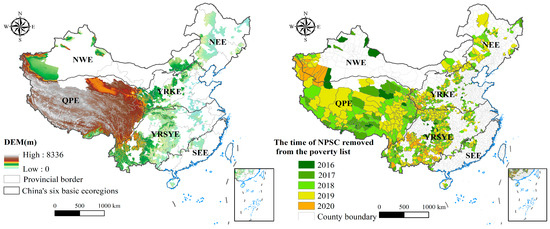
Figure 1.
Geographical location of NPSCs and timeline of poverty alleviation. QPE, SEE, NWE, YRSYE, NEE, and YRKE represent Qinghai–Tibet Plateau Ecoregion, Southeast Ecoregion, Northwest Ecoregion, Yangtze River and Sichuan–Yunnan Key Ecoregion, Northeast Ecoregion, and Yellow River Key Ecoregion, respectively.
2.2. Dataset Sources and Processing
The datasets for 2005, 2013, and 2020 were used to assess ecosystem vulnerability in the NPSCs (Table 1). Data on land use/cover were gathered from Earth System Science Data ((https://essd.copernicus.org/articles/13/3907/2021/) (accessed on 24 November 2023). Terrain data, including the Digital Elevation Model (DEM) and topographic relief amplitude, were downloaded from NASA’s LP DAAC and Chinese Academy of Sciences (CAS). The National Cryosphere Desert Data Center (NCDC) and CAS contributed to the Harmonized World Soil Database V1.2, from which soil data were collected. Monthly vegetation coverage data were obtained from National Tibetan Plateau Data Center ((https://www.tpdc.ac.cn/zh-hans/data/f3bae344-9d4b-4df6-82a0-81499c0f90f7) (accessed on 22 September 2023). The normalized difference vegetation index (NDVI) was calculated on the Google Earth Engine and provided by Yang et al. (2019) [52]). Water yield and soil conservation were provided by Li et al. (2022) [53]) and Li et al. (2023) [54], respectively.

Table 1.
Data used in this study and their sources.
Since administrative divisions changed between 2005 and 2020, we utilized the 2014 administrative region data from the Ministry of Civil Affairs (http://xzqh.mca.gov.cn) (accessed on 2 November 2023) (Table 1). County-level grain yield data for 2005, 2013, and 2020 were sourced from the statistical yearbooks of multiple provinces and cities within the NPSCs.
This study generated ecosystem vulnerability maps for the NPSCs (2005–2020), selecting 2005, 2013, and 2020 based on data availability. The habitat condition index (HCI) was computed using topography, soil, and vegetation data. Elevation data (30 m resolution) were processed with ArcGIS 10.8 slope analysis tool. The upper soil layer (0–30 cm) was chosen for its higher organic carbon content, reflecting the vegetation litter concentration. Vegetation coverage was averaged from May to September to match China’s growing season.
To optimize structural detail and spatial variation, 30 m resolution land use data were partitioned into 4 km grids for ecosystem structure index (ESI) analysis. Arcpy divided the study area’s land use data into 6,016,059 grid cells per year. Fragstats 4.2 computed patch indices, while ArcGIS’s raster calculator assessed landscape heterogeneity and connectivity. Land use types (bare land, cropland, forest, grassland, impervious surfaces, shrubland, water bodies, glaciers) had over 90% classification accuracy, ensuring the reliability of the data.
In 2015, the national ecological function zones were classified into nine types, including water conservation, biodiversity protection, soil conservation, windbreak and sand fixation, flood regulation and storage, agricultural and forest product provision, metropolitan clusters, and key town clusters. The 832 national poverty-stricken counties cover 76.52% of these zones. Focusing on ecosystem vulnerability, we calculated four ecosystem functions: water yield, grain productivity, carbon storage, and soil conservation. For grain productivity, cropland data were extracted from reclassified land use data, and county-level NDVI sums were calculated using zonal statistics. Grid-level grain productivity was derived by integrating county-level grain yield data in ArcGIS. Carbon storage was estimated using literature-derived carbon density values for eight river basins (Table S1) and the InVEST model. The processed data were aggregated into secondary indicators at a 1 km resolution to ensure consistency and comparability. The Geodetector method was used to analyze driving factors of ecosystem vulnerability changes, including natural factors (precipitation, temperature, woodland proportion) and socio-economic factors (population density, GDP, built-up land proportion).
This comprehensive data processing approach enables the robust analysis of ecosystem vulnerability and its drivers, offering a solid basis for spatial and temporal comparisons. The annual results consist of the following steps (Figure 2):
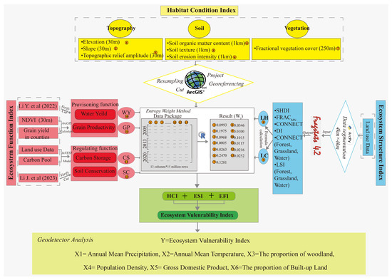
Figure 2.
Overall technical workflow of this study (Sources: data from Li, et al. (2022) [53], Li, et al. (2023) [54]).
2.3. Quantifying Ecosystem Vulnerability
In this study, ecosystem vulnerability is conceptualized as an inherent attribute of ecosystems, indicating their proneness to adverse impacts from external pressures. Based on previous research [58,59,60], we selected evaluation indicators that align with the existing habitat–structure–function framework, while considering the unique characteristics of the study area and the availability of data.
Ecosystem vulnerability was measured from three aspects, habitat condition (HC), ecosystem structure (ES), and ecosystem function (EF), by integrating multiple ecosystem characteristics. Habitat conditions are essential for the proper functioning of regional ecosystems and present the eco-geographical environment characterized by topography, vegetation, and soil [61]. As significant characteristics of ecosystems, this study primarily illustrates the structure and function of ecosystems at the landscape scale, including a range of landscape pattern indicators and ecosystem services [62,63]. Overall, regions characterized by superior habitat conditions, a complex ecosystem structure, and a robust ecosystem function capacity exhibit greater stability and resilience, which ultimately reduces ecosystem vulnerability [64]. The ecosystem vulnerability index (EVI) was calculated as follows:
where HCI, ESI, and EFI refer to the habitat condition index, ecosystem structure index, and ecosystem function index, respectively, which were normalized to [0, 1]. whci, wesi, and wefi represent the weights of HCI, ESI, and EFI. The entropy weight method was employed to calculate the weights of the different indices (Table 2).
Table 2.
Ecosystem variation assessment indicators and weights.
The entropy weight method (EWM) is commonly used to assess the dispersion of values in decision-making. In contrast to diverse subjective weighting models, the EWM’s paramount benefit lies in its ability to circumvent the influence of human bias on the assignment of indicator weights, thereby bolstering the objectivity of the comprehensive evaluation outcomes [65,66]. In this method, m indicators and n samples are set in the evaluation, and the measured value of the i-th indicator in the j-th sample is recorded as xij. Thus, n samples are extracted from a 10 km × 10 km grid in the study area, with m indicators covering three years (2005, 2013, 2020). Each year, there were about 46 × 105 samples per indicator. Due to irregular boundaries, the total sample count over three years is approximately 15 × 106, represented as one column in EWM.
The first step is the standardization of the measured values [67,68]. The standardized value of the i-th index in the j-th sample is denoted as pij, and its calculation method is as follows:
where is a dimensionless value, X is the actual value of the indicator, and Xmin and Xmax are the minimum and maximum actual values of the indicator during 2005–2020, respectively. Positive indicates that the indicator requires positive standardization, as higher values indicate greater ecosystem vulnerability. In contrast, Negative indicates that the indicator requires negative standardization, as higher values indicate lower ecosystem vulnerability.
In the EWM, the entropy value Ei of the i-th index is defined as follows:
In the actual evaluation using the EWM, pij·lnpij = 0 is generally set when pij = 0 for convenience of calculation.
The range of the entropy value Ei is [0, 1]. The larger Ei is, the greater the differentiation degree of index i is, and more information can be derived. Hence, higher weight should be given to the index. Therefore, in the EWM, the calculation method of weight wi is as follows:
2.3.1. Habitat Condition
The quality of a habitat is fundamental to ensuring that species or populations have access to the resources and circumstances they require to survive and reproduce [69]. Habitat loss can reduce biodiversity and increase the risk of ecosystem degradation. Meanwhile, ecosystem degradation may exacerbate habitat loss [70]. Therefore, habitat conditions can act as an inherent indicator of ecosystem vulnerability. Altitude, slope, topography, soil, and fractional vegetation cover were chosen as metrics to describe habitat conditions.
where hck and whck are the standardized value and weight of the k-th habitat condition indicator, respectively.
2.3.2. Ecosystem Structure
We investigated the vulnerability of ecosystem structure using landscape heterogeneity (LH) and landscape connectivity (LC). Grid analysis was chosen as the best approach for landscape structure analysis [71,72,73]. Given that the significant feature size of patch alteration under the targeted poverty alleviation program is around 20 m [74], we believe the 30 m resolution land use data we utilized are appropriate. Considering the dependence of structure analysis on the size of the sampling blocks, we conducted a preliminary test to investigate the scale effects, varying the block size from 1 km to 20 km. Block sizes of 4 km were selected because they can retain sufficient structural information and display the spatial variations in landscape patterns [75]. According to earlier research, a 4 km spatial scale shows a considerable general variance in the evaluation of landscape indices, which is advantageous for the comprehensive retention of specific land use data [76].
Shannon’s diversity index (SHDI) and mean patch fractal dimension (FRACMN) were utilized to measure landscape heterogeneity. Landscape connectance (CONNECT), division index (DIVISION) and landscape shape index (LSI) were recognized as metrics reflecting the connectivity of the entire landscape (WEC) and patches with significant ecological functions (forest, water, grassland) (SPC). The following are the formulas used to calculate landscape heterogeneity and connectivity:
where LH and LC, respectively, denote landscape heterogeneity and landscape connectivity in the NPSCs. SHDI, FRACMN, CONNECT, and DI are all landscape-level metrics, and CONNECTforest, LSIforest, CONNECTwater, LSIwater, CONNECTgrassland, and LSIgrassland are all class-level metrics. And wlh and wlc are the weight of the LH and LC, respectively.
The Arcpy module in Python 2.7 and Fragstats 4.2 [77] were used to acquire the values of the ecosystem structural metrics.
2.3.3. Ecosystem Function
Ecosystem functions are divided into four groups by the Millennium Ecosystem Assessment (MEA): provisioning, regulating, supporting, and cultural services [78]. Xie et al. (2017) [79] identified four primary and eleven secondary categories of ecosystem services within China. This study assesses changes in ecosystem functions by focusing on four crucial ecosystem processes: carbon storage, soil conservation, grain productivity, and water yield. We utilized the results from Li et al. (2023) [54] and Li et al. (2022) [53] as proxies for water yield and soil conservation, respectively. Li et al. (2023) [54] applied ANUSPLIN (ANUS-PRE) and MODIS-ET to compute ecosystem water yield and evaluate uncertainty using the three-cornered hat (TCH) method. To measure soil conservation services, Li et al. (2022) [53] used the Revised Universal Soil Loss Equation (RUSLE) model. Xu et al. (2023) [80] attested to the robustness and dependability of their findings in pertinent research.
Grain Productivity Accounting
Grain productivity and NDVI have been found to be strongly correlated in prior research [81,82]. To determine grid-level grain yield, we used the ratio of the total number of county-level NDVIs to the pixel NDVI and the county-level grain yield. The following is the expression for the calculation formula:
where Gi is the grain productivity of grid i (t), Gsum refers to the total grain output of a county, NDVIi means the NDVI value of grid i of cropland, and NDVIsum represents the summation of the NDVI values of all croplands within a county.
Carbon Storage Accounting
In this study, the carbon storage module of the InVEST model is utilized to analyze carbon storage in the NPSCs. The calculation formula is as follows [83]:
In the formula, C refers to the total carbon storage of the terrestrial ecosystem; i refers to a certain land use type; Si refers to the area of a certain land use type; Ci refers to the total carbon density of the land use type at i; and Ci,above, Ci,below, Ci,soil, and Ci,dead represent the density of above-ground biomass carbon (AGC), below-ground biomass carbon (BGC), soil organic carbon (SOC), and dead organic carbon (DOC), respectively. Details regarding specific carbon density pools are provided in Table S1.
2.4. Geodetector Analysis Method
The Geodetector method quantitatively assesses the degree to which the spatial distribution of geostatistical variables aligns with that of an independent variable [84,85]. The core concept is that if factor X is associated with Y, they will display similar spatial distributions. The method uses the power of the determinant () to reflect the spatial correlation between factors X and Y, as shown in the following equation:
where N is the number of samples in the study area; is the number of samples in zone h of factor X; is the total variance of Y in the study area; is the variance of Y within zone h of factor X; and L is the number of zones of factors X. is the within sum of variances, and is the total sum of variances. The greater the value of is, the more factor X explains Y, and vice versa. We utilized the GD package in R 4.3.3 for computation, and the data were classified using the optimal procedure from the GD package [86].
3. Results
3.1. Spatiotemporal Variation in Ecosystem Vulnerability Index in the NPSCs
With a mean EVI of 0.381, 0.379, and 0.376 for the NPSCs in 2005, 2013, and 2020, respectively, there has been a gradual decline in ecosystem vulnerability over time. With a rise of 101,200 km2, the percentage of low-EVI (<0.3) regions increased slightly from 44.6% to 46.8%, whereas the percentage of medium-EVI (between 0.3 and 0.6) areas decreased by 96,600 km2, from 33.1% in 2005 to 31.0% in 2020 (Figure 3a). The region with a high EVI (>0.6) saw hardly any change. Ecosystem vulnerability decreased (ΔEVI < 0) by around 55.8% of the NPSCs between 2005 and 2020, with major reductions in Inner Mongolia, Gansu, Ningxia, Shaanxi, Chongqing, Guizhou, Hunan, and Anhui (Figure 3b). Meanwhile, Xizang Autonomous Region (Tibet) and Qinghai Province showed an increase in ecosystem vulnerability (ΔEVI > 0). At different stages, the EVI reduction was more noticeable between 2013 and 2020 than it was between 2005 and 2013. In comparison to the −0.0013 (±0.0152) from 2005 to 2013, the average ΔEVI from 2013 to 2020 was −0.0029 (±0.0151), more than twice as high. Additionally, there was a remarkable expansion of areas where the EVI had declined. The proportion of these areas increased from 49.6% during 2005–2013 to 58.7% during 2013–2020.
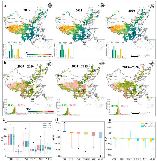
Figure 3.
Distribution of the ecosystem vulnerability index (EVI) and the ΔEVI for the NPSCs. (a) EVI in 2005, 2013, and 2020; (b) ΔEVI in 2005–2020, 2005–2013, and 2013–2020. (a) The bar charts shown in the lower left corner depict the area of the EVI. (b) The pixel distribution plots in the lower left corner represent the number of pixels for ΔEVI. (c) EVI values for different ecoregions in 2005, 2013, and 2020, (d) ΔEVI values for different ecoregions during 2005–2020, and (e) ΔEVI values for different ecoregions during 2005–2013 and 2013–2020. (c) The boxes display the median value and lower 25% and upper 75% percentiles, the dots represent the mean value, and the whiskers are extended to the limit of the 1.5-fold interquartile range (IQR). (d,e) The bar heights show the mean value, and error bars show one standard deviation. The significance of the differences in the EVI and ΔEVI among ecoregions was tested using the Welchi and Tamhena test, and the letters in each bar show the results of multiple comparisons of the mean EVI and ΔEVI with p < 0.05. (c–e) QPE, SEE, NWE, YRSYE, NEE, and YRKE represent Qinghai–Tibet Plateau Ecoregion, Southeast Ecoregion, Northwest Ecoregion, Yangtze River and Sichuan–Yunnan Key Ecoregion, Northeast Ecoregion, and Yellow River Key Ecoregion, respectively.
Geographically, low-EVI (<0.3) areas were mostly found in the eastern, southern, and northeastern sections of the NPSC area, specifically in the Heilongjiang, Hunan, Anhui, and Guangxi provinces (Figure 3a). A high EVI (>0.6) was routinely seen in western regions, such as Qinghai, Tibet, and western Sichuan. To provide more detailed insights, the differences in EVI and ΔEVI were analyzed across China’s six basic ecoregions (i.e., QPE, SEE, NWE, YRSYE, NEE, and YRKE, as shown in Figure 1), which serve as the terrestrial basic units designated by the Ministry of Natural Resources (http://www.creva.org.cn/index.php?m=content&c=index&a=show&catid=44&id=8956) (accessed on 7 March 2025). According to the EVI values, ecosystem vulnerability was ranked in the following order: QPE > NWE > NEE > YRKE > YRSYE > SEE. The QPE (Qinghai–Tibet Plateau Ecoregion) had the highest EVI (0.519 ± 0.158 in 2020), which was nearly triple as high as the lowest EVI of the SEE (Southeast Ecoregion) (0.161 ± 0.025 in 2020) (Figure 3c). From 2005 to 2020, only the QPE region saw an increase in ΔEVI (0.003 ± 0.010), whereas other NPSC ecoregions had ΔEVIs ranging from −0.002 to −0.018 (Figure 3d), showing decreased vulnerability. The YRKE (Yellow River Key Ecoregion) had the greatest substantial reduction, with a ΔEVI of −0.018 ± 0.018, followed by NEE (−0.012 ± 0.014), YRSYE (−0.007 ± 0.019), NEW (−0.005 ± 0.019), and SEE (−0.002 ± 0.016). However, there were differences between the periods before and after 2013. Except for the QPE, all other ecoregions showed a significant decrease in ecosystem vulnerability before 2013. Since 2013, ecosystem vulnerability decreased significantly in the YRSYE (Yangtze River and Sichuan–Yunnan Key Ecoregion), YRKE, and QPE, whereas the NWE (Northwest Ecoregion) witnessed a considerable rise, with a ΔEVI of 0.0019 ± 0.124 (Figure 3e).
3.2. Spatiotemporal Evolution of Ecosystem Vulnerability Indicators
Figure 4 shows that the west-to-east gradient of the habitat condition index (HCI), ecosystem sensitivity index (ESI), and ecosystem function index (EFI) reveals considerable regional disparities. Due to their dry environment and high altitude, regions in the QPE (HCI: 0.526 ± 0.1583) and NWE (HCI: 0.368 ± 0.1127) had poor habitat conditions and an above-average HCI. The ESI varied somewhat between ecoregions, with the QPE having the highest at 0.768 ± 0.1703. This status is largely attributed to the inadequate vegetation and wide barren ground in the northwestern QPE. Except for the SEE (0.401 ± 0.0640) and YRSYE (0.506 ± 0.0825), all ecoregions had EFI values that were more or less above average, indicating greater functional vulnerability in the northern half of the NPSCs (Figure S1).
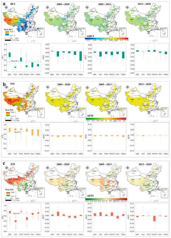
Figure 4.
Distribution of and variation in the ecosystem vulnerability indicators of the NPSCs. Spatial patterns of the standardized mean values of ecosystem vulnerability indicators and their changes in the national poverty-stricken counties. (a) HCI: habitat condition index; (b) ESI: ecosystem structure index; (c) EFI: ecosystem function index. (a–c) The boxes display the median value and lower 25% and upper 75% percentiles, the dots represent the mean value, and the whiskers are extended to the limit of the 1.5-fold interquartile range (IQR). The lines depict the overall mean values of the entire NPSC area. The bar heights represent the mean value, and the error bars show one standard deviation.
Overall, between 2005 and 2020, the ΔHCI (−0.0036 ± 0.016) and ΔESI (−0.01 ± 0.069) were both lower than zero, showing improvements in habitat and ecosystem structure, whereas the ΔEFI (0.0036 ± 0.064) was greater than zero, indicating an increase in ecosystem function vulnerability. The results suggest that the overall decrease in ecosystem vulnerability inside the NPSCs over the course of 15 years was mostly caused by the decreased vulnerability in habitat and ecosystem structure. However, the situation after 2013 is more worthy of attention, with the ΔEFI being −0.0246 (±0.069) and the ΔHCI and the ΔESI being 0.0022 (±0.013) and 0.0004 (±0.056), respectively. This indicates that the improvement in ecosystem function after 2013 played a decisive role in reducing the ecosystem vulnerability of the NPSCs during 2013–2020.
Compared to the period before 2013, the ΔEFI of all ecoregions in the NPSCs decreased during 2013–2020, especially in the QPE, YRSYE, and YRKE. The ΔEFI in the QPE went from 0.0322 (±0.0349) to −0.0154 (±0.0409), in YRSYE went from 0.0456 (±0.0735) to −0.0674 (±0.1035), and in YRKE went from 0.0222 (±0.0512) to −0.0086 (±0.0467) throughout the two periods 2005–2013 and 2013–2020 (Figure 4c). Therefore, the changes in the QPE, YRSYE, and YRKE warrant our close attention.
3.3. Modes of Ecosystem Vulnerability Variation in the NPSCs
We identified eight modes of ecosystem vulnerability changes based on the possible combinations of the ecosystem vulnerability indicators’ variations (increase or decrease). The area proportions of the eight modes during 2005–2020 are shown in Figure 5a. The most prevalent mode, HCIdownESIdownEFIup, accounted for 34.5% of the observed modes. Following this, the next modes were HCIdownESIupEFIup, HCIupESIdownEFIup, and HCIdownESIdownEFIdown, with area proportions of 22.7%, 10.6%, and 8.8%, respectively. According to Figure 5b, the top four modes during 2005–2013 were the same as those during 2005–2020. However, from 2013 to 2020, the modes appeared in a different order: HCIdownESIdownEFIdown (17.3%), HCIdownESIdownEFIup (15.9%), HCIdownESIupEFIdown (14.5%), and HCIdownESIupEFIup (12.1%). Furthermore, as the area of the EFIdown-related modes increased after 2013, the area proportions of the eight modes became more balanced.
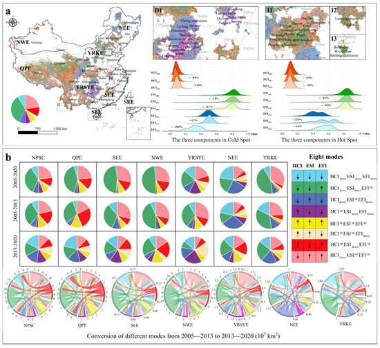
Figure 5.
Spatial distributions and composition proportions of eight ecosystem vulnerability modes for the NPSCs during 2005–2020 (the upper row) and those for the six ecoregions in different periods (the below row). (a) The HCI, ESI, and EFI constitute the ecosystem vulnerability index (EVI). The arrows labeled “up” and “down” represent an increasing and decreasing trend, respectively. Four main hot spots in the areas where the EVI most obviously decreased and increased were selected to show the changes in each component of the EVI. Cold spots, D1, included 41 poverty-stricken counties from the Guizhou, Chongqing, Hunan, Hubei, and Anhui provinces, and the hot spots were I1 in the Sichuan, Shaanxi, and Henan provinces (22 poverty-stricken counties), I2 in the Yunnan provinces (3 poverty-stricken counties), and I3 in the Hainan provinces (4 poverty-stricken counties). The ridge plots display the normalized values of the HCIvul, ESIvul, and EFIvul for hot spots in 2005, 2013, and 2020, and the percentages of increase or decrease for each of these values are used to reflect their contributions to the changes in the EVI. (b) Pie charts depict the proportional areas of eight ecosystem vulnerability modes across various time periods in the six NPSC ecoregions.
From a geographical perspective, the ecoregions demonstrated various predominant modes of change before and after 2013. In the QPE, the HCIdownESIdownEFIdown mode experienced the most substantial growth in area proportion, increasing from 5.09% (pre-2013) to 21.6% (post-2013), which was largely transferred from HCIupESIdownEFIup and HCIdownESIdownEFIup. For the YRSYE, the area of the HCIupESIdownEFIdown mode increased from 2.83% to 22.31% due to the decrease in HCIdownESIdownEFIup and HCIdownESIupEFIup, indicating a trade-off between the HCI and EFI in this region. As for the YRKE, during 2013–2020, the HCIdownESIupEFIdown mode’s area expanded most significantly, rising from 10.8% to 18.8%, largely due to the transition from HCIdownESIdownEFIup to HCIdown ESIupEFIup.
We also looked at the fluctuation in certain vulnerability indicators for both hot spots (increased EVI, I1, I2, and I3) and cold spots (decreased EVI, D1) (Figure 5a and Figure S2), where vulnerability showed significant changes during 2005–2020. Generally, cold spots shifted from a pre-2013 HCIdownESIdownEFIup to post-2013 HCIupESIdownEFIdown, while hot spots consistently exhibited HCIdownESIdownEFIup. In other words, both cold spots and hot spots saw considerable EFI changes. Specifically, the EFI change in hot spots during 2005–2013 was up to +23%, while in cold spots, it was −38% during 2013–2020. As a result, EFI modification had a major impact on locations experiencing large ecosystem vulnerability changes between 2005 and 2020.
3.4. Possible Causes for Ecosystem Vulnerability Changes
Because the QPE, YRSYE, and YRKE revealed substantial variations in ecosystem vulnerability before and after 2013, Geodetector was used to determine whether the probable drivers changed spatiotemporally. In accordance with previous research [87,88,89,90], we identified the influencing factors (Table S2), which included natural factors such as annual mean precipitation (AMP), annual mean temperature (AMT), and the proportion of woodland (PWL), as well as socioeconomic factors such as population density (PD), gross domestic product (GDP), and the proportion of built-up land (PBL).
As seen in Figure 6, the contributions of the variables differed between ecoregions. Between 2005 and 2020, the primary factors were AMP for the QPE, PWL, and YRSYE, and AMP and AMT for the YRKE. This suggested that natural factors were the major determinants of ecosystem vulnerability in the three ecoregions, which supported the findings of previous research [88,91,92,93]. Interestingly, the GDP became the second most powerful factor since 2013. Furthermore, correlation analysis (Figure 7) indicates a substantial negative association between the EVI and GDP, implying that ecosystem vulnerability reduces as GDP increases. This conclusion suggests that economic growth can benefit ecosystems, lending support to the notion that China’s impoverished areas have achieved a degree of a “win–win” situation in terms of poverty alleviation and environmental protection. This finding validates previous data from local or regional research [94,95,96,97].
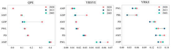
Figure 6.
The contribution rate q for the QPE, YRSYE, and YRKE from 2005 to 2020. Note: q ϵ [0, 1]. QPE, YRSYE, and YRKE represent Qinghai–Tibet Plateau Ecoregion, Yangtze River and Sichuan–Yunnan Key Ecoregion, and Yellow River Key Ecoregion, respectively. PBL, the proportion of built-up land. AMT, mean annual temperature. GDP, gross domestic product. PWL, the proportion of woodland. PD, population density. AMP, annual mean precipitation.
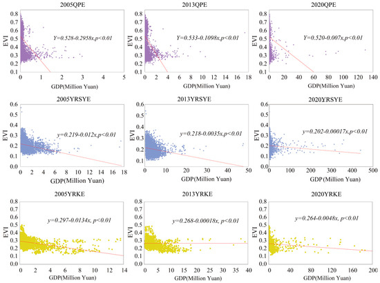
Figure 7.
Correlation analysis between EVI and GDP for QPE, YRSYE, and YRKE from 2005 to 2020. QPE, YRSYE, and YRKE represent Qinghai–Tibet Plateau Ecoregion, Yangtze River and Sichuan–Yunnan Key Ecoregion, and Yellow River Key Ecoregion, respectively.
According to the environmental Kuznets curve, environmental pollution and ecological degradation cannot be adequately regulated or repaired until the per capita GDP surpasses USD 10,000 (about RMB 70,000) [98]. Despite the fact that the per capita GDP was less than this USD 10,000 threshold in 2005 or 2013, it appears that these three regions experienced different states during the study period. This shows that China has discovered methods to possibly shorten the environmental Kuznets curve in disadvantaged areas [99]. China’s policy investments in poverty alleviation and ecological protection have greatly boosted economic growth in impoverished areas, while also enhancing local ecological environment quality [100].
For instance, the QPE has received major financial and project-based support. Between 2005 and 2013, the national government allocated RMB 7.5 billion for the first phase of the Three-River-Source Ecological Protection and Construction Project (TREPCCP). Following that, between 2013 and 2020, the state funded RMB 16.06 billion for the second phase of the TREPCCP (Figure S3 and Table S4) (https://www.gov.cn/jrzg/2014-02/06/content_2580724.htm) (accessed on 7 March 2025). Evidently, such large investments may stimulate the development of eco-friendly enterprises, creating more eco-jobs for the poor in the Qinghai–Tibet Plateau region, which is helpful in achieving the goals of poverty alleviation and ecological protection [19,95]. Similarly, in the YRSYE there has been a surge in the implementation of poverty alleviation and ecological projects or measures from 2013 to 2020. These include relocating more impoverished individuals from inhospitable locations, boosting ecological compensation, and allocating additional projects (i.e., New Round of Returning Farmland to Forests and Grasslands, Rocky Desertification Control) [47,101]. As documented, these interventions stimulated economic growth while enhancing ecological quality in the YRSYE’s impoverished regions [88,92]. The Yellow River Key Ecoregion is an important ecological barrier and rural development zone in China. The eco-priority development model for the ecological industry in the YRKE has led to a more diversified financing channel and a more comprehensive ecological compensation mechanism in the region after 2013. Poverty reduction policies have fostered the specialization of agricultural production and the development of non-agricultural surplus labor, effectively broadening the channels for farmers to increase their income [102] and enhancing opportunities for rural livelihood capital [103]. Additionally, due to the implementation of numerous ecological projects, such as soil and water conservation initiatives (e.g., dams, terraces, forestation, and grassland coverage), the sediment load of the Yellow River has been reduced, effectively mitigating soil erosion by 40% [104]. In terms of poverty alleviation and ecological protection, the YRKE has made remarkable achievements.
Furthermore, this study reveals that precipitation and temperature also influence changes in ecosystem vulnerability. Adequate moisture and warmer temperatures contribute to the lengthening of the vegetation growing season and the enhancement of photosynthesis, which promote ecosystem restoration. However, some regional differences in climate change impacts may not have been detected in our study. For instance, the frequent extreme drought events in Yunnan Province have significantly affected ecosystem vulnerability, leading to vegetation degradation, water scarcity, and biodiversity loss [105]. Additionally, the warming–wetting trend in the Yellow River Basin, while alleviating water resource pressures to some extent, may also trigger new ecological issues, such as changes in vegetation types and increased soil erosion [106]. These regional climate change impacts require further investigation to comprehensively understand the driving mechanisms of ecosystem vulnerability.
4. Discussion
4.1. Policy Implications
The poverty-stricken areas in China highly overlap with ecologically vulnerable regions. Between 2013 and 2020, the policy objectives of the Chinese government were integrated under the interventions of targeted poverty alleviation and ecological protection. Against this backdrop, we observed a decreasing trend in the ecosystem vulnerability of China’s 832 national poverty-stricken counties from 2005 to 2020, with a more pronounced decline during the period from 2013 to 2020. This highlights the synergistic effect of China’s targeted poverty alleviation and ecological protection policies. Our analysis of driving factors reveals that economic improvement is the main driver of reduced ecosystem vulnerability in poverty-stricken areas. For ecological protection policies to succeed, they need sustained support from local residents, especially those in poverty [107]. Ecological protection goals must be integrated with economic development that ensures residents’ long-term livelihoods, as they may return to previous practices if subsidies stop or project conclude [108].
Overall, the Chinese government has achieved targets for poverty alleviation and ecological protection, implementing a “win–win” policy (Figure 8). This has effectively broken the vicious cycle of poverty and ecosystem vulnerability in areas that account for 46% of China’s landmass [95]. On the one hand, targeted poverty alleviation has addressed individual poverty issues through five unconventional strategies (e.g., business development, education support, social security, resettlement, and ecological compensation) [109], thereby promoting economic growth among the impoverished population. On the other hand, poverty-oriented ecological protection policies have tackled regional ecological problems and have contributed to solving regional poverty issues. The ecological poverty alleviation approach encompasses five primary strategies: participation in ecological engineering projects, the implementation of ecological compensation policies, the establishment of public welfare ecological positions, the promotion of eco-friendly industries, and the implementation of ecological relocation programs [110,111,112]. China has demonstrated significant success in these practices, including employing over 1.1 million impoverished individuals as forest rangers and resettling 9.6 million impoverished households through ecological relocation [47]. This demonstrates that ecological protection projects should not only provide ecological benefits but also bring long-term economic benefits to residents, a method that can also promote the implementation of the United Nations Sustainable Development Goals, such as protecting ecosystems and eradicating poverty [113].
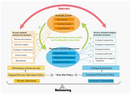
Figure 8.
Policy intervention mechanisms for balancing poverty alleviation and ecosystem vulnerability in poverty-stricken areas. The “+” symbol represents a promoting effect, while the “−” symbol represents an inhibitory effect.
Our research demonstrates the synergy between policy objective formulation and outcomes in China, offering a model for other countries facing poverty traps through coordinated policy objectives and implementation. Policy objectives focus on institutional mechanisms that integrate environmental protection with poverty alleviation and development. Since 2015, China has enhanced its ecological civilization system, ensuring ecological protection through comprehensive laws and regulations [114]. This policy was later integrated with a proposed targeted poverty alleviation policy, promoting the combined development of poverty alleviation and ecological protection while emphasizing ecological principles throughout the process. This innovation introduced a new mechanism for ecological poverty alleviation and established the framework for green poverty reduction [115]. However, due to differences in social systems, economic scales, and the presence of unstable factors such as war, social conflict, and climate change, it remains uncertain whether other countries can achieve the unification of these two policy objectives through government-led top-level design or other models [116,117].
In terms of policy implementation, countries and regions face distinct poverty and ecological degradation challenges due to varying geographical and climatic conditions [118]. Economic disparities further influence factors such as asset distribution, access to farmland, labor availability, land tenure, livelihood strategies, risk perception, family lifecycle, and food security [119,120]. In regions with vulnerable ecosystems and a limited population self-development capacity, where environmental and poverty issues are intertwined, ecological construction and poverty alleviation cannot solely focus on balancing ecological and economic benefits [121]. The environmental pressures from economic development must be addressed, as policy interactions may reduce their effectiveness. Therefore, establishing policy instruments that can coordinate the two objectives is particularly important. Taking the ecological compensation system as an example, it is a product of the conflict stage between the environment and economic development, compensating for the external diseconomy of the environment and coordinating the balance of economic development rights and ecological protection responsibilities among regions, river basins, and different populations [47,101]. It can shorten the time for the environmental Kuznets curve to reach its peak, reduce the height of the peak, and optimize the curve shape [122]. Many studies have explored the positive role of ecological compensation policies in poverty reduction, providing a possibility for the effective coordination of the relationship between ecological protection and poverty alleviation development. Examples include the RUPES (Rewarding the Upland Poor for Ecosystem Services) project in Asia, which focuses on the poverty-alleviating effects of environmental services [123]; the Western Altiplano Natural Resources Management Project in Guatemala, which targets poor households and emphasizes the impact of market-based natural resource management strategies on the livelihoods of the poor [124]; and the National Environmental Management Project in El Salvador, which explicitly combines poverty reduction targets with market-oriented natural resource management, aiming to benefit small-scale poor households [125]. These can serve as important references for development.
The following specific recommendations can serve as a reference for other developing countries: (1) Develop a series of policy frameworks that integrate poverty eradication and ecological protection, ensuring the continuity of coordinated intervention policies. These frameworks should include clear goals, timelines, and monitoring mechanisms to track progress and adapt strategies as needed. (2) Adopt a pilot-then-scale-up approach, given the limited resources available for poverty alleviation and ecological conservation. Pilot projects can help identify best practices and optimize resource allocation before broader implementation. (3) Prioritize severely affected regions and tailor strategies to local conditions. This involves conducting detailed assessments of regional ecological and socioeconomic conditions to design context-specific interventions. (4) Emphasize the role of the government, as poverty eradication and ecological protection are, to a certain extent, public goods that markets cannot adequately address. Governments should establish regulatory frameworks, provide financial support, and foster multi-stakeholder collaboration to ensure effective implementation. (5) Engage in international mechanisms, such as carbon trading and partnerships with environmental funds (e.g., the Green Climate Fund), to secure sustainable financing for ecological compensation. Participation in global carbon markets can monetize carbon sequestration, while collaboration through platforms like the UNFCCC can enhance knowledge sharing and capacity building for effective implementation.
While China’s achievements deserve recognition, the lasting effectiveness of combining environmental protection with poverty control requires thorough analysis. Official statistics show that from 2013 to 2018, total government spending on poverty relief exceeded RMB 1.34 trillion, successfully assisting 65.89 million people [126]. This equals an average cost of RMB 20,362 per person through basic fund transfers alone, not including hidden expenses or environmental impacts. However, the effectiveness of short-term, high-intensity government fiscal investments may have developmental limitations. On the one hand, interventions are time-bound. For example, after the subsidy period for the Grain-for-Green Program ends, some farmers (particularly those in impoverished regions and households) may revert to farming due to livelihood pressures [127,128]. On the other hand, ecosystems follow their own succession patterns and spatial interdependencies, necessitating long-term studies to assess the impacts of short-term interventions. For instance, the Grain-for-Green Program has resulted in monoculture forests with reduced ecological resilience [129], while the large-scale afforestation on the Loess Plateau has altered hydrological cycles, significantly reducing midstream runoff in the Yellow River [130], exacerbating water scarcity and endangering downstream water demand.
4.2. Policy Suggestions
The future direction should focus on transitioning poverty alleviation and ecological protection policies towards rural revitalization. This strategy will preserve the benefits of poverty reduction and environmental protection while reducing the dangers of ecological degradation and poverty recurrence [131,132,133,134]. Hot spot analysis reveals areas that require ongoing monitoring. We have identified 29 counties in Shaanxi, Sichuan, Chongqing, Yunnan, and Hainan as regions with significant increases, with 10 of these being key counties for rural revitalization efforts, highlighting their role in this process (Table S3). Hot Spot I1, located primarily in the Qinba mountainous region, has seen improved natural ecological conditions following the “National Territorial Functional Zoning Plan” of 2010. This has enhanced its water conservation and soil retention capabilities [135]. However, ecological restoration projects have exposed issues such as excessive vegetation restoration and low-quality cover over time, which harm the ecosystem [136,137]. Hot Spot I2, mainly in Yunnan province, faces challenges due to ecological conservation redline and terrain limitations, resulting in a low overall rate of suitable farmland. This has led to excessive land development in some counties, weakening the province’s ecological environment [138,139]. Hot Spot I3, situated in the inland highlands of Hainan Island, has experienced a rapid expansion of rubber plantations since the 1980s, leading to the logging of significant natural forests [140]. By 2010, the fraction of natural woods dropped from 41.4% to 24.2%. While rubber plantations have helped the local economy and rural communities, they have diminished the availability of ecosystem services. Furthermore, the usage of chemical pesticides, tree diseases, and insect pests worsened due to these plantations, and these factors, as well as climate change, continue to pose ecological concerns for the island [141].
Overall, China must adopt a diversified strategy for ecological regeneration in its previously disadvantaged regions to address the issue of the long-term sustainability of policy interventions. In extremely sensitive places such as the Qinghai–Tibet Plateau Ecoregion and the Northwest Ecoregion, implementing sustainable agriculture techniques such as fallow land and rest grazing is critical for green development [142,143,144]. Furthermore, policy-driven compensatory measures and effective ecological monitoring for ecological revival must be maintained [145,146]. In locations with considerably enhanced ecosystem vulnerability, such as the Qinba mountains and the Yunnan border area, greater political attention should be paid to detecting and managing the dangers of re-impoverishment and environmental degradation. Eco-tourism development and carbon trading should be promoted in biologically rich places such as the Southeastern Ecoregion [147,148]. Stabilizing the livelihoods of the impoverished population, completely transforming their environmentally harmful production practices, and reinforcing the concept of ecological conservation are essential to lift poverty-stricken areas out of poverty and to make ecologically vulnerable regions more resilient.
Additionally, the habitat–structure–function framework employed in this article has effectively revealed the significant trade-off between ecosystem functions and habitat conditions. For instance, in hot spots, the primary modes of vulnerability change are HCIdownESIdownEFIup and HCIupESIdownEFIdown. The ongoing decline in forest vegetation diversity, coupled with rising greenhouse gas emissions and factors such as the use of impermeable materials and urban expansion, contribute to habitat fragmentation. This poses a threat to the stability of regional atmospheric and water cycles [149,150,151]. With the increased frequency of major catastrophes, the trade-off between habitat and ecosystem function is anticipated to worsen with time. Future policy development should prioritize the analysis of trade-offs and synergies within ecosystems to support the accomplishment of long-term goals. By striking an adequate scientific balance between ecosystem function and habitat condition, ecosystem trade-offs may still be reconciled and an ideal regional ecological management plan developed. Future studies should develop a more complete evaluation methodology based on each region’s primary biological roles and habitat characteristics. For example, in the Yellow River Key Ecoregion, special attention should be paid to the balance of water yield and vegetation covering, which is crucial for addressing local ecological rehabilitation in rural development [152,153,154].
4.3. Limitation and Future Research Directions
This study examined the spatiotemporal variations in ecosystem vulnerability in China’s impoverished counties but has several limitations. First, some indicators fail to fully capture regional ecosystem characteristics. For example, in karst areas, vegetation coverage as an indicator is limited and short-sighted due to their slow soil formation and unique hydrological structures, which hinder vegetation restoration [155]. Second, critical indicators like soil moisture and biodiversity were excluded due to data unavailability, despite their importance for ecosystem health assessment. Future research should prioritize data collection and sharing to enhance the evaluation framework’s comprehensiveness. Third, the analysis used a 1 km × 1 km resolution, but ecosystem vulnerability modes may differ between small and large regions, and their connections cannot be simplified as mere cumulative effects. Future studies should explore scale-dependent trade-offs to better understand these mechanisms. Fourth, while the Geodetector and correlation analyses identified potential drivers of ecosystem vulnerability changes and indirectly affirmed the “win–win” outcomes of China’s poverty eradication strategy, a more nuanced understanding is needed. For instance, decomposing GDP growth into fiscal transfers and incomes from primary, secondary, and tertiary industries could reveal the complex mechanisms behind this “win–win” scenario.
5. Conclusions
We measured the ecosystem vulnerability in China’s impoverished areas from 2005 to 2020 using the habitat–structure–function assessment framework. The ecosystem vulnerability showed a persistent declining trend and significant differences among the six terrestrial basic ecoregions studied over a 15-year period. Notably, after 2013, the Qinghai–Tibet Plateau Ecoregion (QPE), the Yangtze River and Sichuan–Yunnan Key Ecoregion (YRSYE), and the Yellow River Key Ecoregion (YRKE) exhibited significant changes. We identified which ecosystem functions significantly contributed to the reduction in ecosystem vulnerability. The predominant mode characterized by HCIdownESIdownEFIup was prevalent across China’s impoverished regions from 2005 to 2020. However, the area proportions of the eight modes became more balanced because the area of the EFIdown-related modes increased after 2013. An analysis of the factors influencing ecosystem vulnerability in impoverished areas revealed that the impact of GDP growth on ecosystem vulnerability has increased since 2013. Financial investments in poverty alleviation and the implementation of ecological protection policies have boosted the economic income of poor areas and have effectively enhanced the ecological environment.
Our research gives credible insights into the ecosystem vulnerability in China’s impoverished areas, which aids in the comprehension of the country’s ecological poverty alleviation policies. It holds significant guiding value for the future of rural and ecological revitalization efforts in China. Furthermore, it serves as an important reference for other developing countries or underdeveloped regions seeking to capitalize on poverty reduction opportunities and benefit from coordinated strategies that link poverty reduction with ecological conservation.
Supplementary Materials
The following supporting information can be downloaded at https://www.mdpi.com/article/10.3390/su17062490/s1, Figure S1: Ecosystem function vulnerability of water yield, soil conservation, grain yield, and carbon storage; Figure S2: Distribution of cold and hot spots of ecosystem vulnerability in the NPSC; Figure S3: Poverty alleviation and ecological protection policies in impoverished areas before and after 2013; Table S1: Carbon storage in diverse river basins [156,157,158,159,160,161,162,163,164,165,166,167,168,169,170,171,172]; Table S2: The variable resolution, descriptions, and data sources; Table S3: List of areas that significantly increase ecosystem vulnerability; Table S4: Poverty alleviation and ecological protection policies before and after 2013.
Author Contributions
Conceptualization, W.L. and Z.M.; methodology, W.L., R.L. and Z.M.; software, W.L. and S.W.; validation, W.L., Z.M. and Q.B.; formal analysis, W.L. and Y.H.; investigation, W.L. and X.M.; resources, W.L.; data curation, W.L. and R.L.; writing—original draft preparation, W.L.; writing—review and editing, R.L., S.W., Y.H. and X.M.; visualization, W.L. and Y.H.; supervision, Z.M.; project administration, Z.M. and W.L.; funding acquisition, Z.M. and W.L. All authors have read and agreed to the published version of the manuscript.
Funding
This research was funded by the Gansu Provincial Department of Natural Resources Science and Technology Innovation Project (Grant No. 202243) and the Gansu Provincial Department of Education excellent graduate “innovation star” program (Grant No. 2023CXZX-112).
Institutional Review Board Statement
This study was conducted in accordance with the Declaration of Helsinki. Ethical review and approval were waived for this study as it does not involve sensitive or vulnerable groups.
Data Availability Statement
The data presented in this study are available on request from the corresponding author due to privacy restrictions.
Acknowledgments
The authors would like to thank the Supercomputing Center of Lanzhou University for their support with the computing activities.
Conflicts of Interest
The authors declare no conflicts of interest.
Abbreviations
The following abbreviations are used in this manuscript:
| EVI | Ecosystem Vulnerability Index |
| NPSC | National Poverty-Stricken County |
| HCI | Habitat Condition Index |
| ESI | Ecosystem Structure Index |
| LH | Landscape Heterogeneity |
| LC | Landscape Connectivity |
| EFI | Ecosystem Function Index |
| WY | Water Yield |
| GP | Grain Productivity |
| CS | Carbon Storage |
| SC | Soil Conservation |
| QPE | Qinghai–Tibet Plateau Ecoregion |
| SEE | Southeast Ecoregion |
| NWE | Northwest Ecoregion |
| YRSYE | Yangtze River and Sichuan–Yunnan Key Ecoregion |
| NEE | Northeast Ecoregion |
| YRKE | Yellow River Key Ecoregion |
| AMP | Annual Mean Precipitation |
| AMT | Annual Mean Temperature |
| PBL | Proportion of Built-up Land |
| PWL | Proportion of Wood Land |
| PD | Population Density |
| GDP | Gross Domestic Product |
References
- UNDP. Human Development Report 2020: The Next Frontier: Human Development and the Anthropocene; United Nations: New York, NY, USA, 2020. [Google Scholar]
- Haider, L.J.; Boonstra, W.J.; Peterson, G.D.; Schlüter, M. Traps and Sustainable Development in Rural Areas: A Review. World Dev. 2018, 101, 311–321. [Google Scholar] [CrossRef]
- Albert, J.S.; Carnaval, A.C.; Flantua, S.G.A.; Lohmann, L.G.; Ribas, C.C.; Riff, D.; Carrillo, J.D.; Fan, Y.; Figueiredo, J.J.P.; Guayasamin, J.M.; et al. Human impacts outpace natural processes in the Amazon. Science 2023, 379, eabo5003. [Google Scholar] [CrossRef]
- UN. Independent Group of Scientists Appointed by the Secretary-General, Global Sustainable Development Report 2023: Times of Crisis, Times of Change: Science for Accelerating Transformations to Sustainable Development; United Nations: New York, NY, USA, 2023. [Google Scholar]
- Lapola, D.M.; Pinho, P.; Barlow, J.; Aragão, L.E.O.C.; Berenguer, E.; Carmenta, R.; Liddy, H.M.; Seixas, H.; Silva, C.V.J.; Silva-Junior, C.H.L.; et al. The drivers and impacts of Amazon forest degradation. Science 2023, 379, eabp8622. [Google Scholar] [CrossRef] [PubMed]
- Pörtner, H.-O.; Scholes, R.J.; Arneth, A.; Barnes, D.K.A.; Burrows, M.T.; Diamond, S.E.; Duarte, C.M.; Kiessling, W.; Leadley, P.; Managi, S.; et al. Overcoming the coupled climate and biodiversity crises and their societal impacts. Science 2023, 380, eabl4881. [Google Scholar] [CrossRef]
- Li, G.; Fang, C.; Li, Y.; Wang, Z.; Sun, S.; He, S.; Qi, W.; Bao, C.; Ma, H.; Fan, Y.; et al. Global impacts of future urban expansion on terrestrial vertebrate diversity. Nat. Commun. 2022, 13, 1628. [Google Scholar] [CrossRef] [PubMed]
- Simkin, R.D.; Seto, K.C.; McDonald, R.I.; Jetz, W. Biodiversity impacts and conservation implications of urban land expansion projected to 2050. Proc. Natl. Acad. Sci. USA 2022, 119, e2117297119. [Google Scholar] [CrossRef]
- Pradhan, P.; Costa, L.; Rybski, D.; Lucht, W.; Kropp, J.P. A Systematic Study of Sustainable Development Goal (SDG) Interactions. Earth’s Future 2017, 5, 1169–1179. [Google Scholar] [CrossRef]
- Masron, T.A.; Subramaniam, Y. Does poverty cause environmental degradation? Evidence from developing countries. J. Poverty 2018, 23, 44–64. [Google Scholar] [CrossRef]
- Aluko, M. Sustainable Development, Environmental Degradation and the Entrenchment of Poverty in the Niger Delta of Nigeria. J. Hum. Ecol. 2006, 15, 63–68. [Google Scholar] [CrossRef]
- Le, W.; Leshan, J. How eco-compensation contribute to poverty reduction: A perspective from different income group of rural households in Guizhou, China. J. Clean. Prod. 2020, 275, 122962. [Google Scholar] [CrossRef]
- Althor, G.; Mahood, S.; Witt, B.; Colvin, R.M.; Watson, J.E. Large-scale environmental degradation results in inequitable impacts to already impoverished communities: A case study from the floating villages of Cambodia. AMBIO 2018, 47, 747–759. [Google Scholar] [CrossRef] [PubMed]
- Zhou, Y.; Guo, L.; Liu, Y. Land consolidation boosting poverty alleviation in China: Theory and practice. Land Use Policy 2019, 82, 339–348. [Google Scholar] [CrossRef]
- Yao, Y.; Fu, B.; Liu, Y.; Wang, Y.; Song, S. The contribution of ecosystem restoration to sustainable development goals in Asian drylands: A literature review. Land Degrad. Dev. 2021, 32, 4472–4483. [Google Scholar] [CrossRef]
- Barbier, E.B. Poverty, development, and environment. Environ. Dev. Econ. 2010, 15, 635–660. [Google Scholar] [CrossRef]
- SCIO. Poverty Alleviation: China’s Experience and Contribution; The State Council Information Office of the People’s Republic of China: Beijing, China, 2021.
- EDCYPAD. Yearbook of China’s Poverty Alleviation and Development; Unity Press: Beijing, China, 2015. [Google Scholar]
- Ran, R.; Ni, Z.; Hua, L.; Li, T. Does China’s poverty alleviation policy improve the quality of the ecological environment in poverty-stricken areas? Front. Environ. Sci. 2022, 10, 1067339. [Google Scholar] [CrossRef]
- Li, C.; Li, S.; Feldman, M.W.; Li, J.; Zheng, H.; Daily, G.C. The impact on rural livelihoods and ecosystem services of a major relocation and settlement program: A case in Shaanxi, China. AMBIO 2018, 47, 245–259. [Google Scholar] [CrossRef]
- Ferraro, P.J.; Simorangkir, R. Conditional cash transfers to alleviate poverty also reduced deforestation in Indonesia. Sci. Adv. 2020, 6, eaaz1298. [Google Scholar] [CrossRef]
- Liu, Q.; Gao, L.; Guo, Z.; Dong, Y.; Moallemi, E.A.; Eker, S.; Yang, J.; Obersteiner, M.; Bryan, B.A. Robust strategies to end global poverty and reduce environmental pressures. One Earth 2023, 6, 392–408. [Google Scholar] [CrossRef]
- Bruckner, B.; Hubacek, K.; Shan, Y.; Zhong, H.; Feng, K. Impacts of poverty alleviation on national and global carbon emissions. Nat. Sustain. 2022, 5, 311–320. [Google Scholar] [CrossRef]
- Wang, K.; Yue, Y.; Chen, H.; Zeng, F. Mechanisims and realization pathways for intergration of scientific poverty alleviation and ecosystem services enhancement. Bull. Chin. Acad. Sci. 2020, 35, 1264–1272. [Google Scholar] [CrossRef]
- Deng, X.; Yan, S.; Song, X.; Li, Z.; Mao, J. Spatial targets and payment modes of win–win payments for ecosystem services and poverty reduction. Ecol. Indic. 2022, 136, 108612. [Google Scholar] [CrossRef]
- Guo, M.; Li, C.; Wang, G.; Innes, J.L. Examining the links between livelihood sustainability and environmental protection in the anti-poverty relocation and settlement program areas: An empirical analysis of Shaanxi, China. Front. Environ. Sci. 2022, 10, 1047223. [Google Scholar] [CrossRef]
- Hu, Y.; Kuhn, L.; Zeng, W.; Glauben, T. Who benefits from payments for ecosystem services? Policy lessons from a forest carbon sink program in China. Ecol. Econ. 2023, 214, 107976. [Google Scholar] [CrossRef]
- Ge, Y.; Hu, S.; Song, Y.; Zheng, H.; Liu, Y.; Ye, X.; Ma, T.; Liu, M.; Zhou, C. Sustainable poverty reduction models for the coordinated development of the social economy and environment in China. Sci. Bull. 2023, 68, 2236–2246. [Google Scholar] [CrossRef]
- Hou, P.; Gao, J.; Chen, Y.; Zhai, J.; Xiao, R.; Zhang, W.; Sun, C.; Wang, Y.; Hou, J. Development process and characteristics of China’s ecological protection policy. Acta Ecol. Sin. 2021, 41, 1656–1667. [Google Scholar] [CrossRef]
- Ran, R.; Hua, L.; Xiao, J.; Ma, L.; Pang, M.; Ni, Z. Can poverty alleviation policy enhance ecosystem service value? Evidence from poverty-stricken regions in China. Econ. Anal. Policy 2023, 80, 1509–1525. [Google Scholar] [CrossRef]
- Zhou, L.; Guan, D.; Yuan, X.; Zhang, M.; Gao, W. Quantifying the spatiotemporal characteristics of ecosystem services and livelihoods in China’s poverty-stricken counties. Front. Earth Sci. 2021, 15, 553–579. [Google Scholar] [CrossRef]
- Guo, Z.; Xie, Y.; Guo, H.; Zhang, X.; Wang, H.; Bie, Q.; Xi, G.; Ma, C. Do the ecosystems of Gansu Province in Western China’s crucial ecological security barrier remain vulnerable? Evidence from remote sensing based on geospatial analysis. J. Clean. Prod. 2023, 402, 137818. [Google Scholar] [CrossRef]
- Díaz, S.; Purvis, A.; Cornelissen, J.H.C.; Mace, G.M.; Donoghue, M.J.; Ewers, R.M.; Jordano, P.; Pearse, W.D. Functional traits, the phylogeny of function, and ecosystem service vulnerability. Ecol. Evol. 2013, 3, 2958–2975. [Google Scholar] [CrossRef]
- Luo, M.; Jia, X.; Zhao, Y.; Zhang, P.; Zhao, M. Ecological vulnerability assessment and its driving force based on ecological zoning in the Loess Plateau, China. Ecol. Indic. 2024, 159, 11658. [Google Scholar] [CrossRef]
- Li, Z.; Chen, X.; Zhen, H. Ecology; Science Press: Beijing, China, 2014. [Google Scholar]
- Xue, L.; Wang, J.; Zhang, L.; Wei, G.; Zhu, B. Spatiotemporal analysis of ecological vulnerability and management in the Tarim River Basin, China. Sci. Total. Environ. 2019, 649, 876–888. [Google Scholar] [CrossRef]
- Zhang, X.; Wang, L.; Fu, X.; Li, H.; Xu, C. Ecological vulnerability assessment based on PSSR in Yellow River Delta. J. Clean. Prod. 2017, 167, 1106–1111. [Google Scholar] [CrossRef]
- Zhang, X.; Liu, K.; Wang, S.; Wu, T.; Li, X.; Wang, J.; Wang, D.; Zhu, H.; Tan, C.; Ji, Y. Spatiotemporal evolution of ecological vulnerability in the Yellow River Basin under ecological restoration initiatives. Ecol. Indic. 2022, 135, 108586. [Google Scholar] [CrossRef]
- Malekmohammadi, B.; Jahanishakib, F. Vulnerability assessment of wetland landscape ecosystem services using driver-pressure-state-impact-response (DPSIR) model. Ecol. Indic. 2017, 82, 293–303. [Google Scholar] [CrossRef]
- Peng, Y.; Welden, N.; Renaud, F.G. A framework for integrating ecosystem services indicators into vulnerability and risk assessments of deltaic social-ecological systems. J. Environ. Manag. 2023, 326, 116682. [Google Scholar] [CrossRef]
- Wan, J.-Z.; Wang, C.-J.; Qu, H.; Liu, R.; Zhang, Z.-X. Vulnerability of forest vegetation to anthropogenic climate change in China. Sci. Total Environ. 2018, 621, 1633–1641. [Google Scholar] [CrossRef]
- Xiang, J.; Li, X.; Xiao, R.; Wang, Y. Effects of land use transition on ecological vulnerability in poverty-stricken mountainous areas of China: A complex network approach. J. Environ. Manag. 2021, 297, 113206. [Google Scholar] [CrossRef]
- Zhang, B.; Li, L. Evaluation of ecosystem service value and vulnerability analysis of China national nature reserves: A case study of Shennongjia Forest Region. Ecol. Indic. 2023, 149, 110188. [Google Scholar] [CrossRef]
- Wu, J.; Chen, B.; Mao, J.; Feng, Z. Spatiotemporal evolution of carbon sequestration vulnerability and its relationship with urbanization in China’s coastal zone. Sci. Total Environ. 2018, 645, 692–701. [Google Scholar] [CrossRef]
- Pan, Z.; Gao, G.; Fu, B. Spatiotemporal changes and driving forces of ecosystem vulnerability in the Yangtze River Basin, China: Quantification using habitat-structure-function framework. Sci. Total Environ. 2022, 835, 155494. [Google Scholar] [CrossRef]
- Qin, B.; Yu, Y.; Ge, L.; Yang, L.; Guo, Y. Does eco-compensation alleviate rural poverty? New evidence from National Key Ecological Function Areas in China. Int. J. Environ. Res. Public Health 2022, 19, 10899. [Google Scholar] [CrossRef] [PubMed]
- Jiangyi, L.; Shiquan, D. Eco-compensation in China: Achievement, experience, and improvement. Environ. Sci. Pollut. Res. 2022, 29, 60867–60884. [Google Scholar] [CrossRef] [PubMed]
- Ma, Z.; Tian, X.; Zhang, P. Could ecological restoration reduce income inequality? An analysis of 290 Chinese prefecture-level cities. AMBIO 2023, 52, 802–812. [Google Scholar] [CrossRef]
- Ren, L.; Li, J.; Li, S.; Li, C.; Daily, G.C. Does China’s major Payment for Ecosystem Services program meet the “gold criteria”? Targeting strategies of different decision-makers. J. Clean. Prod. 2020, 275, 122667. [Google Scholar] [CrossRef]
- Liu, Y.; Guo, Y.; Zhou, Y. Poverty alleviation in rural China: Policy changes, future challenges and policy implications. China Agric. Econ. Rev. 2018, 10, 241–259. [Google Scholar] [CrossRef]
- Zhou, Y.; Li, Y.; Liu, Y. The nexus between regional eco-environmental degradation and rural impoverishment in China. Habitat Int. 2020, 96, 102086. [Google Scholar] [CrossRef]
- Yang, J.; Dong, J.; Xiao, X.; Dai, J.; Wu, C.; Xia, J.; Zhao, G.; Zhao, M.; Li, Z.; Zhang, Y.; et al. Divergent shifts in peak photosynthesis timing of temperate and alpine grasslands in China. Remote Sens. Environ. 2019, 233, 111395. [Google Scholar] [CrossRef]
- Li, Y.; Chen, P.; Niu, Y.; Liang, Y.; Wei, T. Dynamics and attributions of ecosystem water yields in China from 2001 to 2020. Ecol. Indic. 2022, 143, 109373. [Google Scholar] [CrossRef]
- Li, J.; He, H.; Zeng, Q.; Chen, L.; Sun, R. A Chinese soil conservation dataset preventing soil water erosion from 1992 to 2019. Sci. Data 2023, 10, 319. [Google Scholar] [CrossRef]
- Yang, J.; Huang, X. The 30 m annual land cover dataset and its dynamics in China from 1990 to 2019. Earth Syst. Sci. Data 2021, 13, 3907–3925. [Google Scholar] [CrossRef]
- You, Z.; Feng, Z.; Yang, Y. Relief degree of land surface dataset of China (1km). Digit. J. Glob. Chang. Data Repos. 2018. [Google Scholar] [CrossRef]
- Gao, J.; Zhang, H.; Zhang, W.; Chen, X.; Shen, W.; Xiao, T.; Zhang, Y. China Regional 250 m Fractional Vegetation Cover Data Set (2000–2023); National Tibetan Plateau Data Center: Beijing, China, 2024. [Google Scholar] [CrossRef]
- Eigenbrod, F.; Gonzalez, P.; Dash, J.; Steyl, I. Vulnerability of ecosystems to climate change moderated by habitat intactness. Glob. Change Biol. 2015, 21, 275–286. [Google Scholar] [CrossRef]
- Schmidt, A.L.; Coll, M.; Romanuk, T.N.; Lotze, H.K. Ecosystem structure and services in eelgrass Zostera marina and rockweed Ascophyllum nodosum habitats. Mar. Ecol. Prog. Ser. 2011, 437, 51–68. [Google Scholar] [CrossRef]
- Hou, W.; Gao, J.; Peng, T.; Wu, S.; Dai, E. Review of ecosystem vulnerability studies in the karst region of Southwest China based on a structure-function-habitat framework. J. Prog. Geogr. 2016, 35, 320–330. [Google Scholar] [CrossRef]
- Yohannes, H.; Soromessa, T.; Argaw, M.; Dewan, A. Spatio-temporal changes in habitat quality and linkage with landscape characteristics in the Beressa watershed, Blue Nile basin of Ethiopian highlands. J. Environ. Manag. 2021, 281, 111885. [Google Scholar] [CrossRef] [PubMed]
- Mitchell, M.G.; Devisscher, T. Strong relationships between urbanization, landscape structure, and ecosystem service multifunctionality in urban forest fragments. Landsc. Urban Plan. 2022, 228, 104548. [Google Scholar] [CrossRef]
- Bai, Y.; Wong, C.P.; Jiang, B.; Hughes, A.C.; Wang, M.; Wang, Q. Developing China’s Ecological Redline Policy using ecosystem services assessments for land use planning. Nat. Commun. 2018, 9, 3034. [Google Scholar] [CrossRef]
- Micheli, F.; Mumby, P.J.; Brumbaugh, D.R.; Broad, K.; Dahlgren, C.P.; Harborne, A.R.; Holmes, K.E.; Kappel, C.V.; Litvin, S.Y.; Sanchirico, J.N. High vulnerability of ecosystem function and services to diversity loss in Caribbean coral reefs. Biol. Conserv. 2014, 171, 186–194. [Google Scholar] [CrossRef]
- Geng, Y.; Liu, L.; Chen, L. Rural revitalization of China: A new framework, measurement and forecast. Socio-Econ. Plan. Sci. 2023, 89, 101696. [Google Scholar] [CrossRef]
- Delgado, A.; Romero, I. Environmental conflict analysis using an integrated grey clustering and entropy-weight method: A case study of a mining project in Peru. Environ. Model. Softw. 2016, 77, 108–121. [Google Scholar] [CrossRef]
- Li, X.; Wei, X.; Huang, Q. Comprehensive entropy weight observability-controllability risk analysis and its application to water resource decision-making. Water SA 2012, 38, 573–579. [Google Scholar] [CrossRef]
- Gorgij, A.D.; Kisi, O.; Moghaddam, A.A.; Taghipour, A. Groundwater quality ranking for drinking purposes, using the entropy method and the spatial autocorrelation index. Environ. Earth Sci. 2017, 76, 269. [Google Scholar] [CrossRef]
- Hall, L.S.; Krausman, P.R.; Morrison, M.L. The habitat concept and a plea for standard terminology. Wildl. Soc. Bull. 1997, 25, 173–182. [Google Scholar]
- Chase, J.M.; Blowes, S.A.; Knight, T.M.; Gerstner, K.; May, F. Ecosystem decay exacerbates biodiversity loss with habitat loss. Nature 2020, 584, 238–243. [Google Scholar] [CrossRef] [PubMed]
- Gong, J.; Sun, P.; Xie, Y.; Qian, D.; Jia, Z. Spatiotemporal change and landscape fragmentation in suzhou oasis using the moving window method. Acta Ecol. Sin. 2015, 35, 6470–6480. [Google Scholar] [CrossRef]
- Zou, L.; Wang, J.; Bai, M. Assessing spatial–temporal heterogeneity of China’s landscape fragmentation in 1980–2020. Ecol. Indic. 2022, 136, 108654. [Google Scholar] [CrossRef]
- Zuo, Q.; Zhou, Y.; Li, Q.; Wang, L.; Liu, J.; He, N. Spatial and temporal variations of landscape ecological risk in the mountainous region of southwestern Hubei Province based on the optimal scale. Chin. J. Ecol. 2023, 42, 1186–1196. [Google Scholar] [CrossRef]
- Li, Y.; Liu, Z.; Li, Y. Spatio-temporal features and driving forces of construction land change in typical poverty-stricken border counties—A case study of Longzhou county in the Guangxi Zhuang Autonomous Region. J. Nat. Resour. 2018, 33, 1291–1303. [Google Scholar] [CrossRef]
- Zhou, D.; Lin, Z.; Lim, S.H. Spatial characteristics and risk factor identification for land use spatial conflicts in a rapid urbanization region in China. Environ. Monit. Assess. 2019, 191, 677. [Google Scholar] [CrossRef]
- Zhou, D.; Xu, J.C.; Wang, L. Land use spatial conflicts and complexity: A case study of the urban agglomeration around Hangzhou Bay, China. Geogr. Res. 2015, 34, 1630–1642. [Google Scholar] [CrossRef]
- McGarigal, K.; Cushman, S.A.; Neel, M.C.; Ene, E. FRAGSTATS v4: Spatial Pattern Analysis Program for Categorical and Continuous Maps. Computer Software Program Produced by the Authors at the University of Massachusetts, Amherst. 2013. Available online: https://fragstats.org/ (accessed on 4 July 2023).
- Reid, W.V.; Mooney, H.A.; Carpenter, S.R.; Chopra, K. Millennium Ecosystem Assessment. Ecosystems and Human Well-Being: Synthesis; Island Press: Washington, DC, USA, 2005. [Google Scholar]
- Xie, G.; Zhang, C.; Zhen, L.; Zhang, L. Dynamic changes in the value of China’s ecosystem services. Ecosyst. Serv. 2017, 26, 146–154. [Google Scholar] [CrossRef]
- Xu, S.; Su, Y.; Yan, W.; Liu, Y.; Wang, Y.; Li, J.; Qian, K.; Yang, X.; Ma, X. Influences of Ecological Restoration Programs on Ecosystem Services in Sandy Areas, Northern China. Remote Sens. 2023, 15, 3519. [Google Scholar] [CrossRef]
- Panek, E.; Gozdowski, D. Relationship between MODIS Derived NDVI and Yield of Cereals for Selected European Countries. Agronomy 2021, 11, 340. [Google Scholar] [CrossRef]
- Panek, E.; Gozdowski, D. Analysis of relationship between cereal yield and NDVI for selected regions of Central Europe based on MODIS satellite data. Remote Sens. Appl. Soc. Environ. 2020, 17, 100286. [Google Scholar] [CrossRef]
- He, C.; Zhang, D.; Huang, Q.; Zhao, Y. Assessing the potential impacts of urban expansion on regional carbon storage by linking the LUSD-urban and InVEST models. Environ. Model. Softw. 2016, 75, 44–58. [Google Scholar] [CrossRef]
- Wang, J.; Xu, C. Geodetector: Principle and prospective. Acta Geogr. Sin. 2017, 72, 116–134. [Google Scholar] [CrossRef]
- Wang, J.-F.; Li, X.-H.; Christakos, G.; Liao, Y.-L.; Zhang, T.; Gu, X.; Zheng, X.-Y. Geographical detectors-based health risk assessment and its application in the neural tube defects study of the Heshun region, China. Int. J. Geogr. Inf. Sci. 2010, 24, 107–127. [Google Scholar] [CrossRef]
- Song, Y.; Wang, J.; Ge, Y.; Xu, C. An optimal parameters-based geographical detector model enhances geographic characteristics of explanatory variables for spatial heterogeneity analysis: Cases with different types of spatial data. GISci. Remote Sens. 2020, 57, 593–610. [Google Scholar] [CrossRef]
- Ge, W.; Deng, L.; Wang, F.; Han, J. Quantifying the contributions of human activities and climate change to vegetation net primary productivity dynamics in China from 2001 to 2016. Sci. Total Environ. 2021, 773, 145648. [Google Scholar] [CrossRef]
- Fang, L.; Wang, L.; Chen, W.; Sun, J.; Cao, Q.; Wang, S.; Wang, L. Identifying the impacts of natural and human factors on ecosystem service in the Yangtze and Yellow River Basins. J. Clean. Prod. 2021, 314, 127995. [Google Scholar] [CrossRef]
- Han, R.; Feng, C.-C.; Xu, N.; Guo, L. Spatial heterogeneous relationship between ecosystem services and human disturbances: A case study in Chuandong, China. Sci. Total Environ. 2020, 721, 137818. [Google Scholar] [CrossRef]
- Peng, Y.; Chen, W.; Pan, S.; Gu, T.; Zeng, J. Identifying the driving forces of global ecosystem services balance, 2000–2020. J. Clean. Prod. 2023, 426, 139019. [Google Scholar] [CrossRef]
- Zhang, Q.; Yuan, R.; Singh, V.P.; Xu, C.-Y.; Fan, K.; Shen, Z.; Wang, G.; Zhao, J. Dynamic vulnerability of ecological systems to climate changes across the Qinghai-Tibet Plateau, China. Ecol. Indic. 2022, 134, 108483. [Google Scholar] [CrossRef]
- Chen, C.; Xu, Y. Spatial heterogeneity of human activities and its driving factors in karst areas of Southwest China over the past 20 years. Front. Environ. Sci. 2023, 11, 1225888. [Google Scholar] [CrossRef]
- Chi, H.; Wu, Y.; Zheng, H.; Zhang, B.; Sun, Z.; Yan, J.; Ren, Y.; Guo, L. Spatial patterns of climate change and associated climate hazards in Northwest China. Sci. Rep. 2023, 13, 10418. [Google Scholar] [CrossRef]
- Cao, S.; Xia, C.; Li, W.; Xian, J. Win–win path for ecological restoration. Land Degrad. Dev. 2021, 32, 430–438. [Google Scholar] [CrossRef]
- Hua, L.; Ran, R.; Xie, M.; Li, T. China’s poverty alleviation policy promoted ecological-economic collaborative development: Evidence from poverty-stricken counties on the Qinghai-Tibet Plateau. Int. J. Sustain. Dev. World Ecol. 2023, 30, 402–419. [Google Scholar] [CrossRef]
- Xu, Y.; Wei, J.; Li, Z.; Zhao, Y.; Lei, X.; Sui, P.; Chen, Y. Linking ecosystem services and economic development for optimizing land use change in the poverty areas. Ecosyst. Health Sustain. 2021, 7, 1877571. [Google Scholar] [CrossRef]
- Yuan, B.; Fu, L.; Zou, Y.; Zhang, S.; Chen, X.; Li, F.; Deng, Z.; Xie, Y. Spatiotemporal change detection of ecological quality and the associated affecting factors in Dongting Lake Basin, based on RSEI. J. Clean. Prod. 2021, 302, 126995. [Google Scholar] [CrossRef]
- Dinda, S. Environmental Kuznets Curve hypothesis: A survey. Ecol. Econ. 2004, 49, 431–455. [Google Scholar] [CrossRef]
- Zhang, J.; Luo, M.; Cao, S. How deep is China’s environmental Kuznets curve? An analysis based on ecological restoration under the Grain for Green program. Land Use Policy 2018, 70, 647–653. [Google Scholar] [CrossRef]
- Mian, Y.; Zeyu, X.; Chusheng, Y. Beyond the Environmental Kuznets Curve: An Empirical Study Taking China’s Poverty Alleviation Campaign as a Quasi-Experiment. Soc. Sci. China 2023, 44, 98–128. [Google Scholar] [CrossRef]
- Zhang, Y.; Guan, D.; Wu, L.; Su, X.; Zhou, L.; Peng, G. How can an ecological compensation threshold be determined? A discriminant model integrating the minimum data approach and the most appropriate land use scenarios. Sci. Total Environ. 2022, 852, 158377. [Google Scholar] [CrossRef]
- Wu, X.; Wang, S.; Fu, B.; Feng, X.; Chen, Y. Socio-ecological changes on the Loess Plateau of China after Grain to Green Program. Sci. Total Environ. 2019, 678, 565–573. [Google Scholar] [CrossRef]
- Zhao, X.; Chen, H.; Zhao, H.; Xue, B. Farmer households’ livelihood resilience in ecological-function areas: Case of the Yellow River water source area of China. Environ. Dev. Sustain. 2022, 24, 9665–9686. [Google Scholar] [CrossRef]
- Deng, L.; Shangguan, Z. High quality developmental approach for soil and water conservation and ecological protection on the loess plateau. Front. Agric. Sci. Eng. 2021, 8, 501–511. [Google Scholar] [CrossRef]
- Zhao, R.; Yang, S.; Sun, H.; Zhou, L.; Li, M.; Xing, L.; Tian, R. Extremeness Comparison of Regional Drought Events in Yunnan Province, Southwest China: Based on Different Drought Characteristics and Joint Return Periods. Atmosphere 2023, 14, 1153. [Google Scholar] [CrossRef]
- Zhang, Q.; Zhu, B.; Yang, J.; Ma, P.; Liu, X.; Lu, G.; Wang, Y.; Yu, H.; Liu, W.; Wang, D. New characteristics about the climate humidification trendin Northwest China. Chin. Sci. Bull. 2021, 66, 3757–3771. [Google Scholar] [CrossRef]
- Huang, L.; Shao, Q.; Liu, J. Forest restoration to achieve both ecological and economic progress, Poyang Lake basin, China. Ecol. Eng. 2012, 44, 53–60. [Google Scholar] [CrossRef]
- Cao, S.; Shang, D.; Yue, H.; Ma, H. A win-win strategy for ecological restoration and biodiversity conservation in Southern China. Environ. Res. Lett. 2017, 12, 044004. [Google Scholar] [CrossRef]
- Liu, Y.; Liu, J.; Zhou, Y. Spatio-temporal patterns of rural poverty in China and targeted poverty alleviation strategies. J. Rural. Stud. 2017, 52, 66–75. [Google Scholar] [CrossRef]
- Lei, M.; Yuan, X.-Y.; Yao, X.-Y. Synthesize dual goals: A study on China’s ecological poverty alleviation system. J. Intergr. Agric. 2021, 20, 1042–1059. [Google Scholar] [CrossRef]
- Feng, Q.; Zhou, Z.; Chen, Q.; Zhu, C.; Zhu, M.; Luo, W.; Wang, J. Quantifying the extent of ecological impact from China’s poverty alleviation relocation program: A case study in Guizhou Province. J. Clean. Prod. 2024, 444, 141274. [Google Scholar] [CrossRef]
- Hu, Z.; Wang, Y. The theoretical innovation and realization mechanism of the ecological poverty alleviation in China. J. Tsinghua Univ. (Philos. Soc. Sci.) 2021, 36, 168–206. [Google Scholar] [CrossRef]
- Feng, Q.; Xia, C.; Yuan, W.; Chen, L.; Wang, Y.; Cao, S. Targeted control measures for improving the environment in a semiarid region of China. J. Clean. Prod. 2019, 206, 477–482. [Google Scholar] [CrossRef]
- Liu, C.; Chen, L.; Vanderbeck, R.M.; Valentine, G.; Zhang, M.; Diprose, K.; McQuaid, K. A Chinese route to sustainability: Postsocialist transitions and the construction of ecological civilization. Sustain. Dev. 2018, 26, 741–748. [Google Scholar] [CrossRef]
- Martinez, C. China’s Transition to an Ecological Civilization: Strategies and Global Implications. Int. Crit. Thought 2024, 14, 176–199. [Google Scholar] [CrossRef]
- Riggirozzi, P. Social Policy, Inequalities and the Battle of Rights in Latin America. Dev. Change 2020, 51, 506–522. [Google Scholar] [CrossRef]
- Mani, S.; Osborne, C.P.; Cleaver, F. Land degradation in South Africa: Justice and climate change in tension. People Nat. 2021, 3, 978–989. [Google Scholar] [CrossRef]
- Engelbrecht, B.M.J.; Comita, L.S.; Condit, R.; Kursar, T.A.; Tyree, M.T.; Turner, B.L.; Hubbell, S.P. Drought sensitivity shapes species distribution patterns in tropical forests. Nature 2007, 447, 80–82. [Google Scholar] [CrossRef]
- Peng, W.; Zheng, H.; Robinson, B.E.; Li, C.; Wang, F. Household Livelihood Strategy Choices, Impact Factors, and Environmental Consequences in Miyun Reservoir Watershed, China. Sustainability 2017, 9, 175. [Google Scholar] [CrossRef]
- Wang, C.; Zhang, Y.; Yang, Y.; Yang, Q.; Kush, J.; Xu, Y.; Xu, L. Assessment of sustainable livelihoods of different farmers in hilly red soil erosion areas of southern China. Ecol. Indic. 2016, 64, 123–131. [Google Scholar] [CrossRef]
- Hou, L.; Xia, F.; Chen, Q.; Huang, J.; He, Y.; Rose, N.; Rozelle, S. Grassland ecological compensation policy in China improves grassland quality and increases herders’ income. Nat. Commun. 2021, 12, 4683. [Google Scholar] [CrossRef] [PubMed]
- Pan, Y.; Dong, F.; Du, C. Is China approaching the inflection point of the ecological Kuznets curve? Analysis based on ecosystem service value at the county level. J. Environ. Manag. 2023, 326, 116623. [Google Scholar] [CrossRef]
- Rosales, R.M.P. Developing Pro-Poor Markets for Environmental Services in the Philippines; International Institute for Environment and Development (IIED): London, UK, 2003. [Google Scholar]
- Bank, W. Guatemala Western Altiplano Natural RESOURCES management Project: Project Appraisal Document; World Bank: Washington, DC, USA, 2003. [Google Scholar]
- Bank, W. El Salvador Natural Resources Management Project: Project Appraisal Document; World Bank: Washington, DC, USA, 2002. [Google Scholar]
- He, Z.; Lan, Y. The sustainability of targeted poverty alleviation: A conceptual analysis framework. Adm. Trib. 2021, 28, 28–38. [Google Scholar] [CrossRef]
- Han, H.; Yu, Y. Environmental Value and Policy Sustainability of Returning Farmland to Forests: A Case Study of Wanzhou, Chongqing. Chin. Rural Econ. 2012, 11, 44–55. [Google Scholar] [CrossRef]
- Lu, H.; Zhou, L.; Chen, Y.; Huang, S.; Ma, B.; Wei, X. Sustainability of Grazing Forbidden Policy in Yanchi, Ningxia, China: A Perspective of Peasant Household. J. Desert Res. 2014, 35, 1065–1071. [Google Scholar]
- Hua, F.; Wang, X.; Zheng, X.; Fisher, B.; Wang, L.; Zhu, J.; Tang, Y.; Yu, D.W.; Wilcove, D.S. Opportunities for biodiversity gains under the world’s largest reforestation programme. Nat. Commun. 2016, 7, 12717. [Google Scholar] [CrossRef]
- Jiang, C.; Guo, H.; Wei, Y.; Yang, Z.; Wang, X.; Wen, M.; Yang, L.; Zhao, L.; Zhang, H.; Zhou, P. Ecological restoration is not sufficient for reconciling the trade-off between soil retention and water yield: A contrasting study from catchment governance perspective. Sci. Total Environ. 2021, 754, 142139. [Google Scholar] [CrossRef]
- Yin, X.; Chen, J.; Li, J. Rural innovation system: Revitalize the countryside for a sustainable development. J. Rural Stud. 2022, 93, 471–478. [Google Scholar] [CrossRef]
- Lyu, R.; Clarke, K.C.; Zhang, J.; Feng, J.; Jia, X.; Li, J. Dynamics of spatial relationships among ecosystem services and their determinants: Implications for land use system reform in Northwestern China. Land Use Policy 2021, 102, 105231. [Google Scholar] [CrossRef]
- Yurui, L.; Yi, L.; Pengcan, F.; Hualou, L. Impacts of land consolidation on rural human–environment system in typical watershed of the Loess Plateau and implications for rural development policy. Land Use Policy 2019, 86, 339–350. [Google Scholar] [CrossRef]
- Luo, K.; Wang, H.; Yan, X.; Ma, C.; Zheng, X.; Wu, J.; Wu, C. Study on trade-offs and synergies of rural ecosystem services in the Tacheng-Emin Basin, Xinjiang, China: Implications for zoning management of rural ecological functions. J. Environ. Manag. 2024, 363, 121411. [Google Scholar] [CrossRef] [PubMed]
- He, X.; Li, W.; Xu, X.; Zhao, X. Spatial-Temporal Evolution, Trade-Offs and Synergies of Ecosystem Services in the Qinba Mountains. Sustainability 2023, 15, 10352. [Google Scholar] [CrossRef]
- Zhang, S.; Zhou, Y.; Yu, Y.; Li, F.; Zhang, R.; Li, W. Using the Geodetector Method to Characterize the Spatiotemporal Dynamics of Vegetation and Its Interaction with Environmental Factors in the Qinba Mountains, China. Remote Sens. 2022, 14, 5794. [Google Scholar] [CrossRef]
- He, T.; Dai, X.; Li, W.; Zhou, J.; Zhang, J.; Li, C.; Dai, T.; Li, W.; Lu, H.; Ye, Y.; et al. Response of net primary productivity of vegetation to drought: A case study of Qinba Mountainous area, China (2001–2018). Ecol. Indic. 2023, 149, 110148. [Google Scholar] [CrossRef]
- Wang, J.; Peng, J.; Zhao, M.; Liu, Y.; Chen, Y. Significant trade-off for the impact of Grain-for-Green Programme on ecosystem services in North-western Yunnan, China. Sci. Total Environ. 2017, 574, 57–64. [Google Scholar] [CrossRef]
- Wang, L.; Zhou, S.; Ouyang, S. The spatial prediction and optimization of production-living-ecological space based on Markov–PLUS model: A case study of Yunnan Province. Open Geosci. 2022, 14, 481–493. [Google Scholar] [CrossRef]
- Li, R.; Zheng, H.; Polasky, S.; Hawthorne, P.L.; O’connor, P.; Wang, L.; Li, R.; Xiao, Y.; Wu, T.; Ouyang, Z. Ecosystem restoration on Hainan Island: Can we optimize for enhancing regulating services and poverty alleviation? Environ. Res. Lett. 2020, 15, 084039. [Google Scholar] [CrossRef]
- Li, R.; Zheng, H.; Zhang, C.; Keeler, B.; Samberg, L.H.; Li, C.; Polasky, S.; Ni, Y.; Ouyang, Z. Rural Household Livelihood and Tree Plantation Dependence in the Central Mountainous Region of Hainan Island, China: Implications for Poverty Alleviation. Forests 2020, 11, 248. [Google Scholar] [CrossRef]
- Yu, L.; Liu, S.; Wang, F.; Liu, Y.; Liu, H.; Wang, Q.; Tran, L.-S.P.; Dong, Y.; Li, W. Strategies for agricultural production management based on land, water and carbon footprints on the Qinghai-Tibet Plateau. J. Clean. Prod. 2022, 362, 132563. [Google Scholar] [CrossRef]
- Zhao, Y.; Chen, D.; Fan, J. Sustainable development problems and countermeasures: A case study of the Qinghai-Tibet Plateau. Geogr. Sustain. 2020, 1, 275–283. [Google Scholar] [CrossRef]
- Wang, X.; Song, J.; Xiao, Z.; Wang, J.; Hu, F. Desertification in the Mu Us Sandy Land in China: Response to climate change and human activity from 2000 to 2020. Geogr. Sustain. 2022, 3, 177–189. [Google Scholar] [CrossRef]
- Liu, H.; Liu, S.; Wang, F.; Liu, Y.; Liu, Y.; Sun, J.; McConkey, K.R.; Tran, L.-S.P.; Dong, Y.; Yu, L.; et al. Identifying ecological compensation areas for ecosystem services degradation on the Qinghai-Tibet Plateau. J. Clean. Prod. 2023, 423, 138626. [Google Scholar] [CrossRef]
- Liu, H.; Liu, S.; Wang, F.; Zhao, Y.; Dong, Y. How to synergize ecological restoration to co-benefit the beneficial contributions of nature to people on the Qinghai-Tibet Plateau? J. Environ. Manag. 2023, 348, 119267. [Google Scholar] [CrossRef]
- Jiang, L.; He, X.; Deng, F. Efficiency evaluation of tourism poverty reducation in Luoxiao Mountain Area in scale of county. Econ. Geogr. 2022, 42, 234–240. [Google Scholar] [CrossRef]
- Zhang, G.; Zhang, N. The effect of China’s pilot carbon emissions trading schemes on poverty alleviation: A quasi-natural experiment approach. J. Environ. Manag. 2020, 271, 110973. [Google Scholar] [CrossRef]
- Zhang, Y.; Gentine, P.; Luo, X.; Lian, X.; Liu, Y.; Zhou, S.; Michalak, A.M.; Sun, W.; Fisher, J.B.; Piao, S.; et al. Increasing sensitivity of dryland vegetation greenness to precipitation due to rising atmospheric CO2. Nat. Commun. 2022, 13, 4875. [Google Scholar] [CrossRef]
- Banks-Leite, C.; Ewers, R.M.; Folkard-Tapp, H.; Fraser, A. Countering the effects of habitat loss, fragmentation, and degradation through habitat restoration. One Earth 2020, 3, 672–676. [Google Scholar] [CrossRef]
- Liu, Y.; Gao, Y.; Liu, L.; Song, C.; Ai, D. Nature-based solutions for urban expansion: Integrating ecosystem services into the delineation of growth boundaries. Habitat Int. 2022, 124, 102575. [Google Scholar] [CrossRef]
- Li, C.; Zhang, Y.; Shen, Y.; Yu, Q. Decadal water storage decrease driven by vegetation changes in the Yellow River Basin. Sci. Bull. 2020, 65, 1859–1861. [Google Scholar] [CrossRef] [PubMed]
- Shen, J.; Zhang, H.; Zhao, Y.; Song, J. An examination of the mitigation effect of vegetation restoration on regional water poverty: Based on panel data analysis of 9 provinces in the Yellow River basin of China from 1999 to 2019. Ecol. Indic. 2023, 146, 109860. [Google Scholar] [CrossRef]
- Wang, L.; Zhu, Q.; Zhang, J.; Liu, J.; Zhu, C.; Qu, L. Vegetation dynamics alter the hydrological interconnections between upper and mid-lower reaches of the Yellow River Basin, China. Ecol. Indic. 2023, 148, 110083. [Google Scholar] [CrossRef]
- Bai, X.; Zhang, S.; Ran, C.; Wu, L.; Du, C.; Dai, L.; Yang, X.; Li, Z.; Xue, Y.; Long, M.; et al. Ten problems and solutions for restoration of karst ecosystem in Southwest China. Bull. Chin. Acad. Sci. 2023, 38, 1903–1914. [Google Scholar] [CrossRef]
- Xu, L.; He, N.; Yu, G. A dataset of carbon density in Chinese terrestrial ecosystems (2010s). China Sci. Data 2018, 4, 90–91. [Google Scholar] [CrossRef]
- Qin, M.; Zhao, Y.; Liu, Y.; Jiang, H.; Li, H.; Zhu, Z. Multi-scenario simulation for 2060 and driving factors of the eco-spatial carbon sink in the beibu gulf urban agglomeration. China Chin. Geogr. Sci. 2023, 33, 85–101. [Google Scholar] [CrossRef]
- Li, X.; Che, L.; Hu, B. Spatio-temporal difference analysis of carbon storage in Beihai secosystem based on FLUS-InVEST models. Bull. Survey. Map. 2023, 117–123. [Google Scholar] [CrossRef]
- Ke, X.; Tang, L. Impact of cascading processes of urban expansion and cropland reclamation on the ecosystem of a carbon storage service in Hubei Province, China. Acta Ecol. Sin. 2019, 39, 672–683. [Google Scholar] [CrossRef]
- Sun, X. Evaluation of Ecosystem Services in Shangri-La Based on InVEST Model. Master’s Thesis, Yunnan Normal University, Kunming, China, 2017. [Google Scholar]
- Li, P.; Chen, J.; Li, Y.; Wu, W. Using the InVEST-PLUS model to predict and analyze the pattern of ecosystem carbon storage in Liaoning Province, China. Remote Sens. 2023, 15, 4050. [Google Scholar] [CrossRef]
- Shi, M.; Wu, H.; Jia, H. Temporal and spatial evolution and prediction of carbon stocks in Yili Valley based on MCE-CA-Markov and InVEST models. J. Agric. Resour. Environ. 2021, 38, 1010–1019. [Google Scholar] [CrossRef]
- Zhu, G.; Qiu, D.; Zhang, Z.; Sang, L.; Liu, Y.; Wang, L.; Zhao, K.; Ma, H.; Xu, Y.; Wan, Q. Land-use changes lead to a decrease in carbon storage in arid region, China. Ecol. Indic. 2021, 127, 107770. [Google Scholar] [CrossRef]
- Zhang, Y.; Shi, X.; Tang, Q. Carbon storage assessment in the upper reaches of the Fenhe river under different land use scenarios. Acta Ecol. Sin. 2021, 41, 360–373. [Google Scholar] [CrossRef]
- Liu, G.; Li, G.; Li, J.; Zhang, Y.; Lu, Q.; Du, S. Study on change in carbon storage and its spatial pattern in Mata Watershed from 1999 to 2016 based on InVEST model. Arid Zone Res. 2021, 38, 267–274. [Google Scholar] [CrossRef]
- Wang, L.; Zhu, R.; Yin, Z.; Chen, Z.; Fang, C.; Lu, R.; Zhou, J.; Feng, Y. Impacts of land-use change on the spatio-temporal patterns of terrestrial ecosystem carbon storage in the Gansu Province, Northwest China. Remote Sens. 2022, 14, 3164. [Google Scholar] [CrossRef]
- Zhu, L.; Song, R.; Sun, S.; Li, Y.; Hu, K. Land use/land cover change and its impact on ecosystem carbon storage in coastal areas of China from 1980 to 2050. Ecol. Indic. 2022, 142, 109178. [Google Scholar] [CrossRef]
- Shi, S. Spatio-Temporal Evolution of Land Use Carbon Storage in the Huang-Huai-Hai Plain. Master’s Thesis, Hubei University, Wuhan, China, 2018. [Google Scholar]
- Zhu, W.; Zhang, J.; Cui, Y.; Zheng, H.; Zhu, L. Assessment of territorial ecosystem carbon storage based on land use change scenario: A case study in Qihe River Basin. Acta Geogr. Sin. 2019, 74, 446–459. [Google Scholar] [CrossRef]
- Li, J.; Xia, S.; Yu, X. Evaluation of carbon storage on terrestrial ecosystem in Hebei Province based on InVEST model. J. Ecol. Rural Environ. 2020, 36, 854–861. [Google Scholar] [CrossRef]
- Liu, J.; Xu, H.; Wang, Y.; Li, H.; Shen, W. Evaluation of ecological risk and carbon fixation from land use change: A case study of Huanghua City, Hebei Province. Chin. J. Eco-Agric. 2018, 26, 1217–1226. [Google Scholar] [CrossRef]
- Li, S. The Dynamics of Ecosystem Services and Their Driving Factors in the Jing-Jin-Ji Region. Ph.D. Thesis, Beijing Forestry University, Beijing, China, 2019. [Google Scholar]
Disclaimer/Publisher’s Note: The statements, opinions and data contained in all publications are solely those of the individual author(s) and contributor(s) and not of MDPI and/or the editor(s). MDPI and/or the editor(s) disclaim responsibility for any injury to people or property resulting from any ideas, methods, instructions or products referred to in the content. |
© 2025 by the authors. Licensee MDPI, Basel, Switzerland. This article is an open access article distributed under the terms and conditions of the Creative Commons Attribution (CC BY) license (https://creativecommons.org/licenses/by/4.0/).