
The Relevance of Financial Development, Natural Resources, Technological Innovation, and Human Development for Carbon and Ecological Footprints: Fresh Evidence of the Resource Curse Hypothesis in G-10 Countries


Abstract
1. Introduction
2. Literature Review

| Financial Development—Ecological Footprint and Carbon Footprint | ||||
|---|---|---|---|---|
| Authors | Countries/Groups and Years | Estimators | Empirical Outcomes | |
| Godil et al. [30] | Turkiye | 1986–2018 | QARDL | FD ↑ EF |
| Omoke et al. [27] | Nigeria | 1971–2014 | NARDL | FD ↓ EF |
| Usman and Hammar [65] | APEC | 1990–2017 | FGLS, AMG, CCEMG | FD ↓ EF |
| Usman and Makhdum [10] | BRICS-T | 1990–2018 | MG, AMG, CCEMG | FD ↑ EF |
| Yao et al. [13] | BRICS and Next-11 | 1995–2014 | GMM | FD ↓ EF |
| Saqib [66] | 63 Emerged and Developed Economies | 1990–2020 | AMG, CCEMG | FD ↓ CF |
| Ashraf et al. [17] | 124 Economies | 1993–2013 | GMM | FD ∩ EF |
| Khan et al. [31] | APEC | 1990–2016 | CCEMG | FD ∩ EF |
| Jahanger et al. [15] | 73 Developing Countries | 1990–2016 | PMG, ARDL | FD ↓ EF |
| Alam et al. [67] | Oman | 1984Q1–2018Q4 | ARDL | Short run FD ↑ CF Long run FD ↓ CF |
| Sun et al. [18] | South Asian | 2010–2018 | CS-ARDL | FD ∩ CF |
| Wang et al. [3] | 14 Developing European Union | 1995–2020 | AMG, CCEMG | FD ↑ EF |
| Naqvi et al. [11] | APEC | 1990–2017 | DK, FMOLS | FD ↑ EF |
| Ozturk et al. [68] | South Asian | 1971–2018 | FMOLS, DOLS | FD ↓ EF |
| Saqib et al. [69] | Top ten countries with the biggest EF | 1990–2109 | CCEMG | FD ↑ EF |
| Yasin et al. [29] | BRICS | 1995–2022 | DK | FD ↓ EF |
| Natural Resource Rent—Ecological Footprint and Carbon Footprint | ||||
| Authors | Countries/Groups and Years | Estimators | Empirical Outcomes | |
| Danish et al. [70] | BRICS | 1992–2016 | FMOLS, DOLS | NR ↓ EF |
| Ahmed et al. [32] | China | 1970–2016 | ARDL | NR ↑ EF NR ↑ CF |
| Ulucak et al. [25] | Top 15 Renewable Energy Consumption Economies | 1996–2018 | PSTR | NR ↑ EF |
| Ahmad et al. [71] | 45 Resource-Rich Countries of Asia | 1990–2018 | POLS, DK | NR ↓ EF |
| Ullah et al. [72] | 73 Developing Countries | 1990–2016 | PMG-ARDL | NR ↑ EF |
| Awosusi et al. [33] | India | 1990–2016 | ARDL | NR ↓ EF |
| Onifade [73] | OECD | 2000–2019 | Panel Quantile | NR ↑ EF |
| Dao et al. [74] | OECD | 2009–2019 | MQR | NR ↑ EF |
| Shittu et al. [75] | BRICS | 1992–2018 | FMOLS, DOLS, FE-OLS | NR ↑ EF |
| Human Development—Ecological Footprint and Carbon Footprint | ||||
| Authors | Countries/Groups and Years | Estimators | Empirical Outcomes | |
| Kassouri and Altintas [41] | MENA | 1990–2016 | CCEMG | HD ↓ EF |
| Pata et al. [1] | Top Ten with Largest EF Economies | 1992–2016 | AMG | HD ↓ EF |
| Liu et al. [42] | G-7 | 1992–2018 | CUP-FM, CUP-BC | HD ↓ EF |
| Qiu and Wan [43] | BRICS | 1995–2019 | CS-ARDL | HD ↓ EF |
| Balsalobre-Lorente et al. [76] | G-7 | 1991–2018 | CUP-FM | HD ↓ EF |
| Nguea and Fotio [77] | 31 African Countries | 1996–2018 | Panel Quantile | HD ↓ EF |
| Technological Innovation—Ecological Footprint and Carbon Footprint | ||||
| Authors | Countries/Groups and Years | Estimators | Empirical Outcomes | |
| Sahoo and Sethi [78] | Newly Industrialized Countries | 1990–2017 | MG, PMG, AMG | TEC ↓ EF |
| Chunling et al. [79] | Pakistan | 1992–2018 | ARDL | TEC ↑ EF |
| Jahanger et al. [15] | Developing Countries | 1990–2016 | PMG-ARDL | TEC ↓ EF |
| Usman and Radulescu, [80] | highest nuclear energy-producing countries | 1990–2019 | AMG, CCEMG | TEC ↑ CF |
| Bashir et al. [81] | Newly Industrialized Countries | 1990–2018 | CS-ARDL | TEC ↓ EF |
| Dai et al. [82] | ASEAN | 1995–2018 | CUP-FM, CUP-BC | TEC ↓ EF |
| Raza et al. [37] | G-20 | 1990–2021 | CS-ARDL | TEC ↓ EF |
| Chopra et al. [83] | 5 high-emitting countries | 1990–2022 | CS-ARDL | TEC ↓ CF |
| Quing et al. [63] | South Asian countries | 1990–2020 | CCEMG | TEC ↓ EF |
| Nathaniel et al. [84] | Emerging Countries | 2000–2020 | AMG | TEC ↓ EF |
| Tiwari et al. [64] | USA | 1990–2021 | ARDL | TEC ↓ EF |
| Globalization—Ecological Footprint and Carbon Footprint | ||||
|---|---|---|---|---|
| Authors | Countries/Groups and Years | Estimators | Empirical Outcomes | |
| Usman et al. [85] | USA | 1985Q1–2014Q4 | ARDL | GL ↑ EF |
| Omoke et al. [27] | Nigeria | 1971–2014 | NARDL | Short run GL ↓ CF Long run GL ↑ CF Short and long-run GL ↓ EF |
| Saud et al. [86] | Belt and Road | 1990–2014 | PMG | GL ↓ EF |
| Wang [47] | Brazil, Russia, India, and China | 1997–2016 | ARDL | GL ↓ EF GL ↓ CF |
| Kirikkaleli et al. [87] | Turkiye | 1985–2017 | FMOLS, DOLS | GL ↑ EF |
| Ansari et al. [88] | Top Renewable Energy-Consuming Countries | 1991–2016 | PMG, FMOLS DOLS | GL ↓ EF |
| Pata [89] | BRIC | 1971–2016 | FARDL | GL ↑ EF |
| Ehigiamusoe et al. [90] | 31 African Nations | 1995–2019 | FMOLS | GL ↑ CO2 GL ≠ EF |
| Hassan et al. [48] | OECD | 1990–2019 | AMG, CCEMG | GL ↑ EF |
| Quing et al. [63] | South Asian | 1990–2020 | AMG, CCEMG | GL ↑ EF |
| Trade Openness—Ecological Footprint and Carbon Footprint | ||||
| Authors | Countries/Groups and Years | Estimators | Empirical Outcomes | |
| Altıntas and Kassouri [41] | 20 EU Countries | 1985–2016 | ARDL | Short run TO ↑ CF Long run TO ↓ CF |
| Lu [54] | 13 Asian Countries | 1973–2014 | PMG | TO ↓ EF |
| Kongbuamai [91] | Thailand | 1974–2016 | ARDL | Short and Long run TO ↑ EF |
| Destek and Sinha [49] | 24 Organization for Economic Co-operation and Development countries | 1980–2014 | MG, FMOLS, DOLS | TO ↓ EF |
| Aydin and Turan [92] | BRICS | 1996–2016 | AMG, CCEMG | TO ↓ EF |
| Dada et al. [52] | Nigeria | 1970–2017 | ARDL | TO ↑ EF |
| Wang et al. [51] | G-7 | 1990–2020 | CS-ARDL | TO ↑ EF |
| Liu et al. [93] | Pakistan | 1980–2017 | ARDL | TO ↓ EF |
| Opuala et al. [53] | West Africa | 1980–2017 | PMG | TO ↑ EF |
| Esmaeili et al. [55] | 19 Energy-Intensive Countries | 1997–2018 | ARDL, CS-ARDL | Short run TO ↑ EF Long run TO ↓ EF |
| Javed et al. [94] | Italy | 1994–2019 | DARDL | TO ↑ EF |
| Abdullahi et al. [95] | Ten ECOWAS Countries | 1980–2022 | PMG | TO ↑ EF |
| Urbanization—Ecological Footprint and Carbon Footprint | ||||
| Authors | Countries/Groups and Years | Estimators | Empirical Outcomes | |
| Ahmed et al. [96] | G-7 | 1971–2014 | CUP-FM, CUP-BC | UB ↑ EF |
| Ahmed et al. [32] | China | 1970–2016 | ARDL | UB ↑ EF |
| Nathaniel et al. [59] | CIVETS | 1990–2014 | AMG | UB ↑ EF |
| Nathaniel and Khan [97] | ASEAN | 1990–2016 | AMG | UB ≠ EF |
| Nathaniel [98] | Indonesia | 1971–2014 | ARDL | UB ↑ EF |
| Salman et al. [56] | ASEAN-4 | 1980–2017 | ARDL | UB ≠ EF |
| Ponce et al. [99] | 100 Countries | 1980–2019 | ARDL | UB ↓ CF |
| Shah et al. [57] | Top 15 Natural Gas Supplier Economies | 2000–2019 | CS-ARDL, AMG | UB ↑ EF |
| Hussain et al. [100] | E-7 | 1992–2020 | FMOLS | UB ↑ EF |
| Aziz et al. [101] | Saudi Arabia | 1991–2021 | ARDL | UB ↑ EF |
| Mehmood [102] | G-11 | 1990–2020 | CS-ARDL | UB ↑ EF |
| Renewable Energy—Ecological Footprint and Carbon Footprint | ||||
| Authors | Countries/Groups and Years | Estimators | Empirical Outcomes | |
| Usman and Radulescu, [80] | Highest Nuclear Energy-Producing Countries | 1990–2019 | AMG, CCEMG | RNW ↓ CF |
| Saqib, [66] | 63 Emerging and Developed Countries | 1990–2020 | AMG, CCEMG | RNW ↓ CF |
| Radmehr et al. [103] | EU | 1995–2018 | Spatial Panel | RNW ↓ EF |
| Rahman et al. [104] | India | 1980–2021 | ARDL | RNW ↓ CF |
| Joof et al. [105] | USA | 1980–2018 | ARDL | RNW ↓ EF |
| Sohag et al. [106] | OECD | 1990–2018 | CS-ARDL | RNW ↓ EF |
| Sethi et al. [107] | BRICS+ | 2000–2020 | NARDL | RNW ↓ EF |
Research Gap
3. Variable Selection, Model Construction, and Methodology
3.1. Variable Selection
3.1.1. Dependent Variables
3.1.2. Independent Variables
3.1.3. Control Variables
3.2. Data and Model Construction
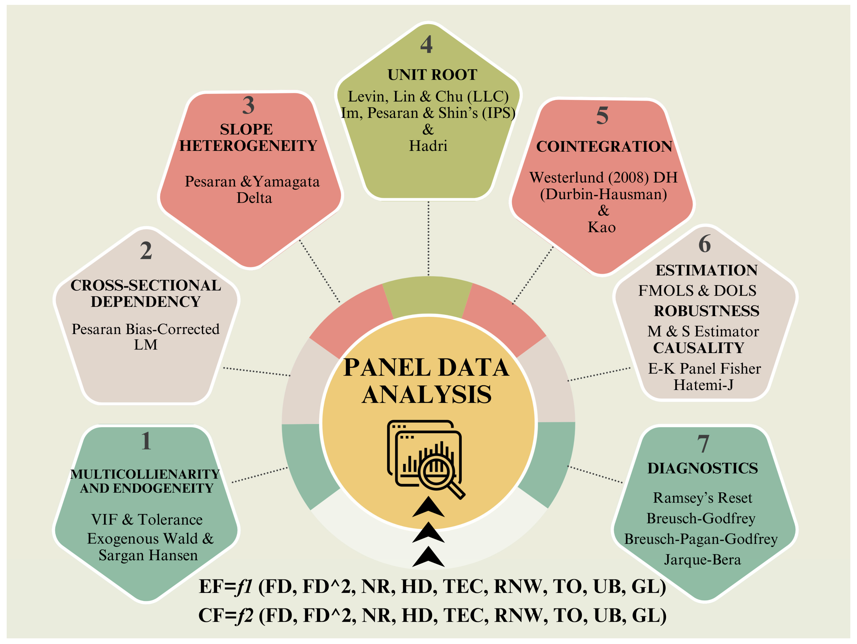
3.3. Methodology
4. Empirical Results
4.1. Initial Statistics
4.2. Main Results
5. Conclusions and Policy Recommendations
Author Contributions
Funding
Institutional Review Board Statement
Informed Consent Statement
Data Availability Statement
Conflicts of Interest
References
- Pata, U.K.; Aydin, M.; Haouas, I. Are natural resources abundance and human development a solution for environmental pressure? Evidence from top ten countries with the largest ecological footprint. Resour. Policy 2021, 70, 101923. [Google Scholar] [CrossRef]
- Guan, C.; Rani, T.; Yueqiang, Z.; Ajaz, T.; Haseki, M.I. Impact of tourism industry, globalization, and technology innovation on ecological footprints in G-10 countries. Econ. Res.-Ekon. Istraz. 2022, 35, 6688–6704. [Google Scholar] [CrossRef]
- Wang, R.; Usman, M.; Radulescu, M.; Cifuentes-Faura, J.; Balsalobre-Lorente, D. Achieving ecological sustainability through technological innovations, financial development, foreign direct investment, and energy consumption in developing European countries. Gondwana Res. 2023, 119, 138–152. [Google Scholar] [CrossRef]
- Pata, U.K.; Yilanci, V. Financial development, globalization and ecological footprint in G7: Further evidence from threshold cointegration and fractional frequency causality tests. Environ. Ecol. Stat. 2020, 27, 803–825. [Google Scholar] [CrossRef]
- Acar, S.; Altintas, N.; Haziyev, V. The effect of financial development and economic growth on ecological footprint in Azerbaijan: An ARDL bound test approach with structural breaks. Environ. Ecol. Stat. 2023, 30, 41–59. [Google Scholar] [CrossRef]
- Majeed, M.T.; Mazhar, M. Financial development and ecological footprint: A global panel data analysis. Pak. J. Commer. Soc. Sci. 2019, 13, 487–514. [Google Scholar]
- Baloch, M.A.; Zhang, J.; Iqbal, K.; Iqbal, Z. The effect of financial development on ecological footprint in BRI countries: Evidence from panel data estimation. Environ. Sci. Pollut. Res. 2019, 26, 6199–6208. [Google Scholar] [CrossRef]
- Khoza, S.; Biyase, M. The symmetric and asymmetric effect of financial development on ecological footprint in South Africa: ARDL and NARDL approach. Front. Environ. Sci. 2024, 12, 1347977. [Google Scholar] [CrossRef]
- Nathaniel, S.P.; Ahmed, Z.; Shamansurova, Z.; Fakher, H.A. Linking clean energy consumption, globalization, and financial development to the ecological footprint in a developing country: Insights from the novel dynamic ARDL simulation techniques. Heliyon 2024, 10, e27095. [Google Scholar] [CrossRef]
- Usman, M.; Makhdum, M.S.A. What abates ecological footprint in BRICS-T region? Exploring the influence of renewable energy, non-renewable energy, agriculture, forest area and financial development. Renew. Energy 2021, 179, 12–28. [Google Scholar] [CrossRef]
- Naqvi, S.A.A.; Hussain, B.; Ali, S. Evaluating the influence of biofuel and waste energy production on environmental degradation in APEC: Role of natural resources and financial development. J. Clean. Prod. 2023, 386, 135790. [Google Scholar] [CrossRef]
- Aytun, C.; Erdogan, S.; Pata, U.K.; Cengiz, O. Associating environmental quality, human capital, financial development, and technological innovation in 19 middle-income countries: A disaggregated ecological footprint approach. Technol. Soc. 2024, 76, 102445. [Google Scholar] [CrossRef]
- Yao, X.; Yasmeen, R.; Hussain, J.; Shah, W.U.H. The repercussions of financial development and corruption on energy efficiency and ecological footprint: Evidence from BRICS and next 11 countries. Energy 2021, 223, 120063. [Google Scholar] [CrossRef]
- Saqib, N. Nexus between renewable and nonrenewable energy consumption and carbon footprints: Evidence from Asian emerging economies. Environ. Sci. Pollut. Res. 2022, 29, 58326–58340. [Google Scholar] [CrossRef] [PubMed]
- Jahanger, A.; Usman, M.; Murshed, M.; Mahmood, H.; Balsalobre-Lorente, D. The linkages between natural resources, human capital, globalization, economic growth, financial development, and ecological footprint: The moderating role of technological innovations. Resour. Policy 2022, 76, 102569. [Google Scholar] [CrossRef]
- Bergougui, B. Investigating the relationships among green technologies, financial development and ecological footprint levels in Algeria: Evidence from a novel Fourier ARDL approach. Sustain. Cities Soc. 2024, 112, 105621. [Google Scholar] [CrossRef]
- Ashraf, A.; Nguyen, C.P.; Doytch, N. The impact of financial development on ecological footprints of nations. J. Environ. Manag. 2022, 322, 116062. [Google Scholar] [CrossRef]
- Sun, Y.; Al-Tal, R.M.; Siddik, A.B.; Khan, S.; Murshed, M.; Alvarado, R. The non-linearity between financial development and carbon footprints: The environmental roles of technological innovation, renewable energy, and foreign direct investment. Econ. Res.-Ekon. Istraz. 2023, 36, 2174153. [Google Scholar] [CrossRef]
- Cai, H.H.; Lee, H.F.; Khan, N.U.; Yuan, Q. Are natural resources a curse, a blessing, or a double-edged sword? Implications for environmental sustainability. J. Environ. Manag. 2024, 367, 122008. [Google Scholar] [CrossRef]
- Qamruzzaman, M. Do natural resources bestow or curse the environmental sustainability in Cambodia? Nexus between clean energy, urbanization, and financial deepening, natural resources, and environmental sustainability. Energy Strategy Rev. 2024, 53, 101412. [Google Scholar] [CrossRef]
- Rong, L.; Wang, Z.; Li, Z. Unraveling the role of financial risk, social globalization and economic risk towards attaining sustainable environment in China: Does resources curse still holds. Resour. Policy 2024, 88, 104375. [Google Scholar] [CrossRef]
- Zhang, L.; Godil, D.I.; Bibi, M.; Khan, M.K.; Sarwat, S.; Anser, M.K. Caring for the environment: How human capital, natural resources, and economic growth interact with environmental degradation in Pakistan? A dynamic ARDL approach. Sci. Total Environ. 2021, 774, 145553. [Google Scholar] [CrossRef]
- Han, G.; Cai, X. The linkages among natural resources, sustainable energy technologies and human capital: An evidence from N-11 countries. Resour. Policy 2024, 90, 104787. [Google Scholar] [CrossRef]
- Shouchang, Y.; Zhonghua, L.; Jintian, W. Exploring the impacts of economic policy uncertainty, natural resources, and energy structure on ecological footprints: Evidence from G-10 nations. Environ. Sci. Pollut. Res. 2023, 30, 45701–45710. [Google Scholar] [CrossRef] [PubMed]
- Ulucak, Z.S.; Ilkay, S.C.; Ozcan, B.; Gedikli, A. Financial globalization and environmental degradation nexus: Evidence from emerging economies. Resour. Policy 2020, 67, 1–8. [Google Scholar] [CrossRef]
- Ullah, S.; Lin, B.; Zhu, R. Developing a new sustainable policy perspective for Pakistan: An intricate nexus between green innovation, financial structure and ecological footprint. Energy 2025, 316, 134496. [Google Scholar] [CrossRef]
- Omoke, P.C.; Nwani, C.; Effiong, E.L.; Evbuomwan, O.O.; Emenekwe, C.C. The impact of financial development on carbon, non-carbon, and total ecological footprint in Nigeria: New evidence from asymmetric dynamic analysis. Environ. Sci. Pollut. Res. 2020, 27, 21628–21646. [Google Scholar] [CrossRef]
- Fan, L.; Usman, M.; Haseeb, M.; Kamal, M. The impact of financial development and energy consumption on ecological footprint in economic complexity-based EKC framework: New evidence from BRICS-T region. In Natural Resources Forum; Blackwell Publishing Ltd.: Oxford, UK, 2024. [Google Scholar] [CrossRef]
- Yasin, I.; Amin, S.; Mehmood, W. Financial development’s role in reducing the ecological footprint of energy consumption in BRICS. In Sustainable Development; Wiley: Hoboken, NJ, USA, 2025. [Google Scholar] [CrossRef]
- Godil, D.I.; Sharif, A.; Rafique, S.; Jermsittiparsert, K. The asymmetric effect of tourism, financial development, and globalization on ecological footprint in Turkey. Environ. Sci. Pollut. Res. 2020, 27, 40109–40120. [Google Scholar] [CrossRef]
- Khan, I.; Hou, F.; Zakari, A.; Irfan, M.; Ahmad, M. Links among energy intensity, non-linear financial development, and environmental sustainability: New evidence from Asia Pacific Economic Cooperation countries. J. Clean. Prod. 2022, 330, 129747. [Google Scholar] [CrossRef]
- Ahmed, Z.; Asghar, M.M.; Malik, M.N.; Nawaz, K. Moving towards a sustainable environment: The dynamic linkage between natural resources, human capital, urbanization, economic growth, and ecological footprint in China. Resour. Policy 2020, 67, 101677. [Google Scholar] [CrossRef]
- Awosusi, A.A.; Adebayo, T.S.; Kirikkaleli, D.; Altuntas, M. Role of technological innovation and globalization in BRICS economies: Policy towards environmental sustainability. Int. J. Sustain. Dev. World Ecol. 2022, 29, 593–610. [Google Scholar] [CrossRef]
- Guan, X.; Wang, Q.; Mansoor, H.; Nadeem, M. The impact of natural resource rent, global value chain participation, and financial development on environmental footprints: A global analysis with fresh evidence. In Natural Resources Forum; Blackwell Publishing Ltd.: Oxford, UK, 2024. [Google Scholar] [CrossRef]
- Deka, A.; Efe-Onakpojeruo, C.C.; Ozdeser, H. Capitalizing on technological innovations and natural resources rent in alleviating ecological footprint in the Sub-Saharan African countries. Resour. Policy 2025, 101, 105462. [Google Scholar] [CrossRef]
- Li, R.; Hu, S.; Wang, Q. Reexamining the impact of natural resource rent and corruption control on environmental quality: Evidence from carbon emissions and ecological footprint in 152 countries. In Natural Resources Forum; Blackwell Publishing Ltd.: Oxford, UK, 2024; Volume 48, pp. 636–660. [Google Scholar] [CrossRef]
- Raza, A.; Habib, Y.; Hashmi, S.H. Impact of technological innovation and renewable energy on ecological footprint in G20 countries: The moderating role of institutional quality. Environ. Sci. Pollut. Res. 2023, 30, 95376–95393. [Google Scholar] [CrossRef]
- Dam, M.M.; Kaya, F.; Bekun, F.V. How does technological innovation affect the ecological footprint? Evidence from E-7 countries in the background of the SDGs. J. Clean. Prod. 2024, 443, 141020. [Google Scholar] [CrossRef]
- Saqib, N.; Ozturk, I.; Usman, M. Investigating the implications of technological innovations, financial inclusion, and renewable energy in diminishing ecological footprints levels in emerging economies. Geosci. Front. 2023, 14, 101667. [Google Scholar] [CrossRef]
- Aydin, C.; Esen, Ö.; Cetintas, Y. Nexus between environmental innovation and ecological footprint in OECD countries: Is there an environmental rebound effect? J. Environ. Stud. Sci. 2024. [Google Scholar] [CrossRef]
- Kassouri, Y.; Altintas, H. Human well-being versus ecological footprint in MENA countries: A trade-off? J. Environ. Manag. 2020, 263, 110405. [Google Scholar] [CrossRef]
- Liu, J.; Loan, V.T.K.; Mousa, S.; Ali, A.; Muda, I.; Cong, P.T. Sustainability and natural resources management in developed countries: The role of financial inclusion and human development. Resour. Policy 2023, 80, 103143. [Google Scholar] [CrossRef]
- Qiu, H.; Wan, Q. Inclusivity between digital trade, human development, and environmental quality: Moderating role of green innovations in BRICS countries. Econ. Res.-Ekon. Istraz. 2023, 36, 2150872. [Google Scholar] [CrossRef]
- Long, X.; Yu, H.; Sun, M.; Wang, X.C.; Klemeš, J.J.; Xie, W.; Wang, Y. Sustainability evaluation based on the Three-dimensional Ecological Footprint and Human Development Index: A case study on the four island regions in China. J. Environ. Manag. 2020, 265, 110509. [Google Scholar] [CrossRef]
- Sharif, A.; Godil, D.I.; Xu, B.; Sinha, A.; Khan, S.A.R.; Jermsittiparsert, K. Revisiting the role of tourism and globalization in environmental degradation in China: Fresh insights from the quantile ARDL approach. J. Clean. Prod. 2020, 272, 1–10. [Google Scholar] [CrossRef]
- Rahman, H.U.; Zaman, U.; Gorecki, J. The role of energy consumption, economic growth and globalization in environmental degradation: Empirical evidence from the BRICS region. Sustainability 2021, 13, 1924. [Google Scholar] [CrossRef]
- Wang, X. Determinants of ecological and carbon footprints to assess the framework of environmental sustainability in BRICS countries: A panel ARDL and causality estimation model. Environ. Res. 2021, 197, 111111. [Google Scholar] [CrossRef] [PubMed]
- Hassan, S.T.; Batool, B.; Wang, P.; Zhu, B.; Sadiq, M. Impact of economic complexity index, globalization, and nuclear energy consumption on ecological footprint: First insights in OECD context. Energy 2023, 263, 125628. [Google Scholar] [CrossRef]
- Destek, M.A.; Sinha, A. Renewable, non-renewable energy consumption, economic growth, trade openness and ecological footprint: Evidence from organization for economic Co-operation and development countries. J. Clean. Prod. 2020, 242, 118537. [Google Scholar] [CrossRef]
- Ali, S.; Yusop, Z.; Kaliappan, S.R.; Chin, L. Trade-environment nexus in OIC countries: Fresh insights from environmental Kuznets curve using GHG emissions and ecological footprint. Environ. Sci. Pollut. Res. 2021, 28, 4531–4548. [Google Scholar] [CrossRef]
- Wang, W.; Rehman, M.A.; Fahad, S. The dynamic influence of renewable energy, trade openness, and industrialization on the sustainable environment in G-7 economies. Renew. Energy 2022, 198, 484–491. [Google Scholar] [CrossRef]
- Dada, J.T.; Adeiza, A.; Noor, A.I.; Marina, A. Investigating the link between economic growth, financial development, urbanization, natural resources, human capital, trade openness and ecological footprint: Evidence from Nigeria. J. Bioecon. 2022, 24, 153–179. [Google Scholar] [CrossRef]
- Opuala, C.S.; Omoke, P.C.; Uche, E. Sustainable environment in West Africa: The roles of financial development, energy consumption, trade openness, urbanization and natural resource depletion. Int. J. Environ. Sci. Technol. 2023, 20, 423–436. [Google Scholar] [CrossRef]
- Lu, W.C. The interplay among ecological footprint, real income, energy consumption, and trade openness in 13 Asian countries. Environ. Sci. Pollut. Res. 2020, 27, 45148–45160. [Google Scholar] [CrossRef]
- Esmaeili, P.; Rafei, M.; Balsalobre-Lorente, D.; Adedoyin, F.F. The role of economic policy uncertainty and social welfare in the view of ecological footprint: Evidence from the traditional and novel platform in panel ARDL approaches. Environ. Sci. Pollut. Res. 2023, 30, 13048–13066. [Google Scholar] [CrossRef] [PubMed]
- Salman, M.; Zha, D.; Wang, G. Interplay between urbanization and ecological footprints: Differential roles of indigenous and foreign innovations in ASEAN-4. Environ. Sci. Policy 2022, 127, 161–180. [Google Scholar] [CrossRef]
- Shah, S.A.R.; Zhang, Q.; Abbas, J.; Balsalobre-Lorente, D.; Pilar, L. Technology, urbanization and natural gas supply matter for carbon neutrality: A new evidence of environmental sustainability under the Prism of COP26. Resour. Policy 2023, 82, 103465. [Google Scholar] [CrossRef]
- Muñoz, P.; Zwick, S.; Mirzabaev, A. The impact of urbanization on Austria’s carbon footprint. J. Clean. Prod. 2020, 263, 121326. [Google Scholar] [CrossRef]
- Nathaniel, S.; Nwodo, O.; Sharma, G.; Shah, M. Renewable energy, urbanization, and ecological footprint linkage in CIVETS. Environ. Sci. Pollut. Res. 2020, 27, 19616–19629. [Google Scholar] [CrossRef]
- Adekoya, O.B.; Oliyide, J.A.; Fasanya, I.O. Renewable and non-renewable energy consumption–Ecological footprint nexus in net-oil exporting and net-oil importing countries: Policy implications for a sustainable environment. Renew. Energy 2022, 189, 524–534. [Google Scholar] [CrossRef]
- Ahmed, Z.; Adebayo, T.S.; Udemba, E.N.; Murshed, M.; Kirikkaleli, D. Effects of economic complexity, economic growth, and renewable energy technology budgets on ecological footprint: The role of democratic accountability. Environ. Sci. Pollut. Res. 2022, 29, 24925–24940. [Google Scholar] [CrossRef]
- Hakkak, M.; Altintaş, N.; Hakkak, S. Exploring the relationship between nuclear and renewable energy usage, ecological footprint, and load capacity factor: A study of the Russian Federation testing the EKC and LCC hypothesis. Renew. Energy Focus 2023, 46, 356–366. [Google Scholar] [CrossRef]
- Qing, L.; Usman, M.; Radulescu, M.; Haseeb, M. Towards the vision of going green in South Asian region: The role of technological innovations, renewable energy and natural resources in ecological footprint during globalization mode. Resour. Policy 2024, 88, 104506. [Google Scholar] [CrossRef]
- Tiwari, S.; Sharif, A.; Sofuoğlu, E.; Nuta, F. A step toward the attainment of carbon neutrality and SDG-13: Role of financial depth and green technology innovation. Res. Int. Bus. Financ. 2025, 73, 102631. [Google Scholar] [CrossRef]
- Usman, M.; Hammar, N. Dynamic relationship between technological innovations, financial development, renewable energy, and ecological footprint: Fresh insights based on the STIRPAT model for Asia Pacific Economic Cooperation countries. Environ. Sci. Pollut. Res. 2021, 28, 15519–15536. [Google Scholar] [CrossRef] [PubMed]
- Saqib, N. Green energy, non-renewable energy, financial development and economic growth with carbon footprint: Heterogeneous panel evidence from cross-country. Econ. Res.-Ekon. Istraživanja 2022, 35, 6945–6964. [Google Scholar] [CrossRef]
- Alam, N.; Hashmi, N.I.; Jamil, S.A.; Murshed, M.; Mahmood, H.; Alam, S. The marginal effects of economic growth, financial development, and low-carbon energy use on carbon footprints in Oman: Fresh evidence from autoregressive distributed lag model analysis. Environ. Sci. Pollut. Res. 2022, 29, 76432–76445. [Google Scholar] [CrossRef]
- Ozturk, I.; Farooq, S.; Majeed, M.T.; Skare, M. An empirical investigation of financial development and ecological footprint in South Asia: Bridging the EKC and pollution haven hypotheses. Geosci. Front. 2024, 15, 101588. [Google Scholar] [CrossRef]
- Saqib, N.; Usman, M.; Ozturk, I.; Sharif, A. Harnessing the synergistic impacts of environmental innovations, financial development, green growth, and ecological footprint through the lens of SDGs policies for countries exhibiting high ecological footprints. Energy Policy 2024, 184, 113863. [Google Scholar] [CrossRef]
- Danish; Ulucak, R.; Khan, S.U.D. Determinants of the ecological footprint: Role of renewable energy, natural resources, and urbanization. Sustain. Cities Soc. 2020, 54, 101996. [Google Scholar] [CrossRef]
- Ahmad, M.; Jiang, P.; Majeed, A.; Umar, M.; Khan, Z.; Muhammad, S. The dynamic impact of natural resources, technological innovations and economic growth on ecological footprint: An advanced panel data estimation. Resour. Policy 2020, 69, 101817. [Google Scholar] [CrossRef]
- Ullah, A.; Ahmed, M.; Raza, S.A.; Ali, S. A threshold approach to sustainable development: Nonlinear relationship between renewable energy consumption, natural resource rent, and ecological footprint. J. Environ. Manag. 2021, 295, 113073. [Google Scholar] [CrossRef]
- Onifade, S.T. Environmental impacts of energy indicators on ecological footprints of oil-exporting African countries: Perspectives on fossil resources abundance amidst sustainable development quests. Resour. Policy 2023, 82, 103481. [Google Scholar] [CrossRef]
- Dao, N.B.; Chu, L.K.; Shahbaz, M.; Tran, T.H. Natural resources-environmental technology-ecological footprint nexus: Does natural resources rents diversification make a difference? J. Environ. Manag. 2024, 359, 121036. [Google Scholar] [CrossRef]
- Shittu, W.; Adedoyin, F.F.; Shah, M.I.; Musibau, H.O. An investigation of the nexus between natural resources, environmental performance, energy security and environmental degradation: Evidence from Asia. Resour. Policy 2021, 73, 102227. [Google Scholar] [CrossRef]
- Balsalobre-Lorente, D.; Nur, T.; Topaloglu, E.E.; Evcimen, C. Assessing the impact of the economic complexity on the ecological footprint in G7 countries: Fresh evidence under human development and energy innovation processes. Gondwana Res. 2024, 127, 226–245. [Google Scholar] [CrossRef]
- Nguea, S.M.; Fotio, H.K. Synthesizing the role of biomass energy consumption and human development in achieving environmental sustainability. Energy 2024, 293, 130500. [Google Scholar] [CrossRef]
- Sahoo, M.; Sethi, N. The dynamic impact of urbanization, structural transformation, and technological innovation on ecological footprint and PM2.5: Evidence from newly industrialized countries. Environ. Dev. Sustain. 2022, 24, 4244–4277. [Google Scholar] [CrossRef]
- Chunling, L.; Memon, J.A.; Thanh, T.L.; Ali, M.; Kirikkaleli, D. The impact of public-private partnership investment in energy and technological innovation on ecological footprint: The case of Pakistan. Sustainability 2021, 13, 10085. [Google Scholar] [CrossRef]
- Usman, M.; Radulescu, M. Examining the role of nuclear and renewable energy in reducing carbon footprint: Does the role of technological innovation really create some difference? Sci. Total Environ. 2022, 841, 156662. [Google Scholar] [CrossRef]
- Bashir, M.A.; Dengfeng, Z.; Filipiak, B.Z.; Bilan, Y.; Vasa, L. Role of economic complexity and technological innovation for ecological footprint in newly industrialized countries: Does geothermal energy consumption matter? Renew. Energy 2023, 217, 119059. [Google Scholar] [CrossRef]
- Dai, J.; Ahmed, Z.; Sinha, A.; Pata, U.K.; Alvarado, R. Sustainable green electricity, technological innovation, and ecological footprint: Does democratic accountability moderate the nexus? Util. Policy 2023, 82, 101541. [Google Scholar] [CrossRef]
- Chopra, R.; Rehman, M.A.; Yadav, A.; Bhardwaj, S. Revisiting the EKC framework concerning COP-28 carbon neutrality management: Evidence from Top-5 carbon embittering countries. J. Environ. Manag. 2024, 356, 120690. [Google Scholar] [CrossRef]
- Nathaniel, S.P.; Solomon, C.J.; Khudoykulov, K.; Fakher, H.A. Linking resource richness, digital economy, and clean energy to ecological footprint and load capacity factor in emerging markets. In Natural Resources Forum; Blackwell Publishing Ltd.: Oxford, UK, 2025. [Google Scholar] [CrossRef]
- Usman, O.; Akadiri, S.S.; Adeshola, I. Role of renewable energy and globalization on ecological footprint in the USA: Implications for environmental sustainability. Environ. Sci. Pollut. Res. 2020, 27, 30681–30693. [Google Scholar] [CrossRef]
- Saud, S.; Chen, S.; Haseeb, A. The role of financial development and globalization in the environment: Accounting ecological footprint indicators for selected one-belt-one-road initiative countries. J. Clean. Prod. 2020, 250, 64–72. [Google Scholar] [CrossRef]
- Kirikkaleli, D.; Adebayo, T.S.; Khan, Z.; Ali, S. Does globalization matter for ecological footprint in Turkey? Evidence from dual adjustment approach. Environ. Sci. Pollut. Res. 2021, 28, 14009–14017. [Google Scholar] [CrossRef] [PubMed]
- Ansari, M.A.; Haider, S.; Masood, T. Do renewable energy and globalization enhance ecological footprint: An analysis of top renewable energy countries? Environ. Sci. Pollut. Res. 2021, 28, 6719–6732. [Google Scholar] [CrossRef]
- Pata, U.K. Linking renewable energy, globalization, agriculture, CO2 emissions and ecological footprint in BRIC countries: A sustainability perspective. Renew. Energy 2021, 173, 197–208. [Google Scholar] [CrossRef]
- Ehigiamusoe, K.U.; Shahbaz, M.; Vo, X.V. How does globalization influence the impact of tourism on carbon emissions and ecological footprint? Evidence from African countries. J. Travel Res. 2023, 62, 1010–1032. [Google Scholar] [CrossRef]
- Kongbuamai, N.; Zafar, M.W.; Zaidi, S.A.H.; Liu, Y. Determinants of the ecological footprint in Thailand: The influences of tourism, trade openness, and population density. Environ. Sci. Pollut. Res. 2020, 27, 40171–40186. [Google Scholar] [CrossRef]
- Aydin, M.; Turan, Y.E. The influence of financial openness, trade openness, and energy intensity on ecological footprint: Revisiting the environmental Kuznets curve hypothesis for BRICS countries. Environ. Sci. Pollut. Res. 2020, 27, 43233–43245. [Google Scholar] [CrossRef]
- Liu, Y.; Sadiq, F.; Ali, W.; Kumail, T. Does tourism development, energy consumption, trade openness and economic growth matter for ecological footprint: Testing the Environmental Kuznets Curve and pollution haven hypothesis for Pakistan. Energy 2022, 245, 123208. [Google Scholar] [CrossRef]
- Javed, A.; Rapposelli, A.; Khan, F.; Javed, A. The impact of green technology innovation, environmental taxes, and renewable energy consumption on ecological footprint in Italy: Fresh evidence from novel dynamic ARDL simulations. Technol. Forecast. Soc. Change 2023, 191, 122534. [Google Scholar] [CrossRef]
- Abdullahi, N.M.; Ibrahim, A.A.; Zhang, Q.; Huo, X. Dynamic linkages between financial development, economic growth, urbanization, trade openness, and ecological footprint: An empirical account of ECOWAS countries. In Environment, Development and Sustainability; Springer: Berlin/Heidelberg, Germany, 2024; pp. 1–28. [Google Scholar] [CrossRef]
- Ahmed, Z.; Zafar, M.W.; Ali, S. Linking urbanization, human capital, and the ecological footprint in G7 countries: An empirical analysis. Sustain. Cities Soc. 2020, 55, 102064. [Google Scholar] [CrossRef]
- Nathaniel, S.; Khan, S.A.R. The nexus between urbanization, renewable energy, trade, and ecological footprint in ASEAN countries. J. Clean. Prod. 2020, 272, 122709. [Google Scholar] [CrossRef]
- Nathaniel, S.P. Ecological footprint, energy use, trade, and urbanization linkage in Indonesia. GeoJournal 2021, 86, 2057–2070. [Google Scholar] [CrossRef]
- Ponce, P.; Álvarez-García, J.; Álvarez, V.; Irfan, M. Analyzing the influence of foreign direct investment and urbanization on the development of private financial system and its ecological footprint. Environ. Sci. Pollut. Res. 2023, 30, 9624–9641. [Google Scholar] [CrossRef]
- Hussain, M.; Abbas, A.; Manzoor, S.; Chengang, Y. Linkage of natural resources, economic policies, urbanization, and the environmental Kuznets curve. Environ. Sci. Pollut. Res. 2023, 30, 1451–1459. [Google Scholar] [CrossRef]
- Aziz, G.; Sarwar, S.; Nawaz, K.; Waheed, R.; Khan, M.S. Influence of tech-industry, natural resources, renewable energy and urbanization towards environment footprints: A fresh evidence of Saudi Arabia. Resour. Policy 2023, 83, 103553. [Google Scholar] [CrossRef]
- Mehmood, U. Assessing the Impacts of Eco-innovations, Economic Growth, Urbanization on Ecological Footprints in G-11: Exploring the Sustainable Development Policy Options. J. Knowl. Econ. 2024, 15, 16849–16867. [Google Scholar] [CrossRef]
- Radmehr, R.; Shayanmehr, S.; Baba, E.A.; Samour, A.; Adebayo, T.S. Spatial spillover effects of green technology innovation and renewable energy on ecological sustainability: New evidence and analysis. Sustain. Dev. 2024, 32, 1743–1761. [Google Scholar] [CrossRef]
- Rahman, M.M.; Mohanty, A.K.; Rahman, M.H. Renewable energy, forestry, economic growth, and demographic impact on carbon footprint in India: Does forestry and renewable energy matter to reduce emission? J. Environ. Stud. Sci. 2024, 14, 415–427. [Google Scholar] [CrossRef]
- Joof, F.; Samour, A.; Ali, M.; Rehman, M.A.; Tursoy, T. Economic complexity, renewable energy and ecological footprint: The role of the housing market in the USA. Energy Build. 2024, 311, 114131. [Google Scholar] [CrossRef]
- Sohag, K.; Husain, S.; Soytas, U. Environmental policy stringency and ecological footprint linkage: Mitigation measures of renewable energy and innovation. Energy Econ. 2024, 136, 107721. [Google Scholar] [CrossRef]
- Sethi, L.; Pata, U.K.; Behera, B.; Sahoo, M.; Sethi, N. Sustainable future orientation for BRICS+ nations: Green growth, political stability, renewable energy and technology for ecological footprint mitigation. Renew. Energy 2025, 244, 122701. [Google Scholar] [CrossRef]
- GFN. Global Footprint Network. 2024. Available online: https://data.footprintnetwork.org (accessed on 20 September 2024).
- IMF. International Monetary Fund. 2024. Available online: https://www.imf.org/ (accessed on 20 September 2024).
- KOF. Swiss Economic Institute. 2023. Available online: https://kof.ethz.ch/ (accessed on 20 September 2024).
- OWID. Our World in Data. 2024. Available online: https://ourworldindata.org/ (accessed on 20 September 2024).
- WB. World Bank. 2023. Available online: https://www.worldbank.org/ (accessed on 20 September 2024).
- Pesaran, M.H.; Ullah, A.; Yamagata, T. A bias-adjusted LM test of error cross-section independence. Econom. J. 2008, 11, 105–127. [Google Scholar] [CrossRef]
- Pesaran, M.H.; Yamagata, T. Testing slope homogeneity in large panels. J. Econom. 2008, 142, 50–93. [Google Scholar] [CrossRef]
- Levin, A.; Lin, C.F.; Chu, C.S.J. Unit root tests in panel data: Asymptotic and finite-sample properties. J. Econom. 2002, 108, 1–24. [Google Scholar] [CrossRef]
- Im, K.S.; Pesaran, M.H.; Shin, Y. Testing for unit roots in heterogeneous panels. J. Econom. 2003, 115, 53–74. [Google Scholar] [CrossRef]
- Hadri, K. Testing for stationarity in heterogeneous panel data. Econom. J. 2000, 3, 148–161. [Google Scholar] [CrossRef]
- Westerlund, J. Panel cointegration tests of the Fisher effect. J. Appl. Econom. 2008, 23, 193–233. [Google Scholar] [CrossRef]
- Kao, C. Spurious regression and residual-based tests for cointegration in panel data. J. Econom. 1999, 90, 1–44. [Google Scholar] [CrossRef]
- Stock, J.H.; Watson, M.W. A simple estimator of cointegrating vectors in higher order integrated systems. Econometrica 1993, 61, 783–820. [Google Scholar] [CrossRef]
- Pedroni, P. Purchasing power parity tests in cointegrated panels. Rev. Econ. Stat. 2001, 83, 727–731. [Google Scholar] [CrossRef]
- Emirmahmutoglu, F.; Kose, N. Testing for Granger causality in heterogeneous mixed panels. Econ. Model. 2011, 28, 870–876. [Google Scholar] [CrossRef]
- Hatemi-j, A. Asymmetric causality tests with an application. Empir. Econ. 2012, 43, 447–456. [Google Scholar] [CrossRef]
- Granger, C.W.; Yoon, G. Hidden cointegration. In Economics Working Paper; University of California: Los Angeles, CA, USA, 2002. [Google Scholar] [CrossRef]
- Tabachnick, B.G.; Fidell, L.S. Using Multivariate Statistics; Pearson Education: Boston, MA, USA, 2001; Available online: https://cir.nii.ac.jp/crid/1130282271473640960 (accessed on 20 September 2024).
- Wooldridge, J.M. Introductory econometrics. J. Contam. Hydrol. 2013, 120–121, 129–140. [Google Scholar] [CrossRef]
- Ze, F.; Yu, W.; Ali, A.; Hishan, S.S.; Muda, I.; Khudoykulov, K. Influence of natural resources, ICT, and financial globalization on economic growth: Evidence from G10 countries. Resour. Policy 2023, 81, 103254. [Google Scholar] [CrossRef]
- Gyamfi, B.A.; Onifade, S.T.; Nwani, C.; Bekun, F.V. Accounting for the combined impacts of natural resources rent, income level, and energy consumption on environmental quality of G7 economies: A panel quantile regression approach. Environ. Sci. Pollut. Res. 2022, 29, 2806–2818. [Google Scholar] [CrossRef]
- Granger, C.W. Some recent developments in a concept of causality. J. Econom. 1988, 39, 199–211. [Google Scholar] [CrossRef]
| Variable | Acronym | Definition | Sources | |
|---|---|---|---|---|
| Dependent | Ecological Footprint | EF | Ecological Footprint (gha per person) | GFN |
| Dependent | Carbon Footprint | CF | Carbon footprint (gha per person) | GFN |
| Independent | Financial Development | FD | Financial Development Index | IMF |
| Independent | Financial Development | FD2 | Financial Development Index | IMF |
| Independent | Natural Resources Rent | NR | Natural resources (% of GDP) | WB |
| Independent | Human Development | HD | Human Development Index | OWID |
| Independent | Technological Innovation | TEC | Patent applications (residents + nonresidents) | WB |
| Control | Renewable Energy Consumption | RNW | % of total final energy consumption | WB |
| Control | Trade Openness | TO | The share of total imports and exports (% of GDP) | WB |
| Control | Urbanization | UB | Urbanization (% of total population) | WB |
| Control | Globalization | GL | KOF Globalization Index | KOF |
| Box plots |  |  | 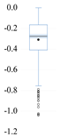 | 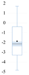 |  | 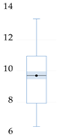 |  | 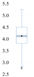 | 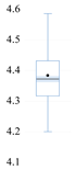 |  |
| Stats. | EF | CF | FD | NR | HD | TEC | RNW | TO | UB | GL |
| Mean | 6.290 | 3.859 | 0.749 | 0.519 | 73.041 | 84022 | 12.686 | 0.893 | 80.517 | 82.291 |
| Median | 5.851 | 3.600 | 0.759 | 0.118 | 62.424 | 16533 | 9.100 | 0.897 | 79.234 | 83.143 |
| Max. | 10.927 | 7.853 | 1.000 | 5.565 | 193.033 | 621453 | 57.900 | 0.967 | 98.153 | 90.929 |
| Min. | 3.461 | 1.910 | 0.354 | 0.008 | 15.723 | 617 | 0.600 | 0.780 | 66.706 | 55.636 |
| Std. Dev. | 1.619 | 1.179 | 0.139 | 0.868 | 39.225 | 151958.7 | 11.842 | 0.037 | 7.886 | 6.673 |
| Skew. | 0.804 | 1.171 | −0.574 | 3.044 | 0.760 | 2.032 | 1.612 | −0.603 | 0.617 | −1.195 |
| Kurt. | 3.047 | 4.404 | 2.962 | 13.730 | 2.810 | 5.910 | 5.579 | 3.044 | 2.904 | 4.642 |
| Jarque–Bera | 39.153 *** | 112.714 *** | 19.958 *** | 2301.673 *** | 35.483 *** | 377.985 | 257.841 *** | 21.992 *** | 23.149 *** | 127.101 *** |
| Obs. | 363 | 363 | 363 | 363 | 363 | 363 | 363 | 363 | 363 | 363 |
| Scatters | 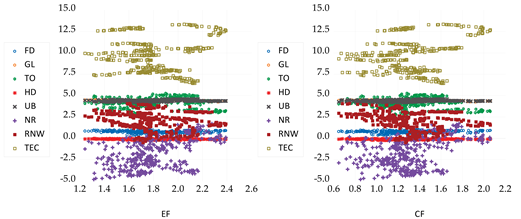 | |||||||||
| 1/VIF | VIF | EF | 1.000 | 0.853 | −0.100 | 0.465 | −0.087 | −0.027 | −0.123 | 0.107 | 0.245 | −0.089 |
| CF | 0.853 | 1.000 | 0.124 | 0.320 | −0.001 | 0.159 | −0.287 | 0.022 | 0.178 | −0.169 | ||
| 0.358 | 2.792 | FD | −0.100 | 0.124 | 1.000 | 0.121 | 0.531 | 0.175 | 0.219 | −0.011 | 0.023 | 0.289 |
| 0.262 | 3.821 | NR | 0.465 | 0.320 | 0.121 | 1.000 | 0.104 | 0.280 | 0.118 | −0.113 | 0.131 | −0.032 |
| 0.250 | 3.998 | HD | −0.087 | −0.001 | 0.531 | 0.104 | 1.000 | −0.037 | 0.411 | 0.424 | 0.424 | 0.648 |
| 0.268 | 3.727 | TEC | −0.027 | 0.159 | 0.175 | 0.280 | −0.037 | 1.000 | −0.154 | −0.795 | −0.106 | −0.592 |
| 0.664 | 1.507 | RNW | −0.123 | −0.287 | 0.219 | 0.118 | 0.411 | −0.154 | 1.000 | 0.235 | −0.017 | 0.278 |
| 0.231 | 4.325 | TO | 0.107 | 0.022 | −0.011 | −0.113 | 0.424 | −0.795 | 0.235 | 1.000 | 0.264 | 0.789 |
| 0.516 | 1.938 | UB | 0.245 | 0.178 | 0.023 | 0.131 | 0.424 | −0.106 | −0.017 | 0.264 | 1.000 | 0.328 |
| 0.858 | 1.165 | GL | −0.089 | −0.169 | 0.289 | −0.032 | 0.648 | −0.592 | 0.278 | 0.789 | 0.328 | 1.000 |
| Mean VIF | (2.909) | EF | CF | FD | NR | HD | TEC | RNW | TO | UB | GL |
| Sargan–Hansen Test for Exogeneity of Instruments | ||||||
|---|---|---|---|---|---|---|
| Instrument Specification: | Instrument Validity | Sargan–Hansen J Statistic | Prob (J-Statistic) | |||
| @DYN(EF,−2) FD(−1) FD2(−1) NR(−1) HD(−1) TEC(−1) RNW(−1) TO(−1) UB(−1) GL(−1) | Model A | 1.462 | 0.226 | |||
| @DYN(CF,−2) FD(−1) FD2(−1) NR(−1) HD(−1) TEC(−1) RNW(−1) TO(−1) UB(−1) GL(−1) | Model B | 2.533 | 0.111 | |||
| H0: The instruments used in this model are valid | ||||||
| Block exogenous Wald test | ||||||
| Hypothesis—H0: Exogenous | X2(1) | Prob. | ||||
| FD | GL | 2.327 | 0.312 | |||
| TO | 0.219 | 0.896 | ||||
| HD | 0.969 | 0.616 | ||||
| UB | 2.211 | 0.331 | ||||
| NR | 0.488 | 0.784 | ||||
| RNW | 0.858 | 0.651 | ||||
| TEC | 3.300 | 0.192 | ||||
| NR | FD | 0.420 | 0.517 | |||
| GL | 0.180 | 0.672 | ||||
| TO | 0.585 | 0.444 | ||||
| HD | 0.963 | 0.326 | ||||
| UB | 0.190 | 0.663 | ||||
| RNW | 2.451 | 0.118 | ||||
| TEC | 1.266 | 0.261 | ||||
| HD | FD | 0.670 | 0.413 | |||
| GL | 2.451 | 0.118 | ||||
| TO | 0.008 | 0.929 | ||||
| UB | 0.298 | 0.585 | ||||
| NR | 0.472 | 0.492 | ||||
| RNW | 0.136 | 0.713 | ||||
| TEC | 0.077 | 0.781 | ||||
| TEC | FD | 4.279 | 0.118 | |||
| GL | 0.205 | 0.903 | ||||
| TO | 1.597 | 0.450 | ||||
| HD | 1.916 | 0.384 | ||||
| UB | 2.046 | 0.360 | ||||
| NR | 2.953 | 0.228 | ||||
| RNW | 1.874 | 0.392 | ||||
| RNW | FD | 0.288 | 0.866 | |||
| GL | 3.485 | 0.175 | ||||
| TO | 1.358 | 0.507 | ||||
| HD | 0.678 | 0.713 | ||||
| UB | 4.533 | 0.104 | ||||
| NR | 1.079 | 0.583 | ||||
| TEC | 2.149 | 0.341 | ||||
| TO | FD | 0.191 | 0.662 | |||
| GL | 0.155 | 0.694 | ||||
| HD | 0.501 | 0.479 | ||||
| UB | 1.248 | 0.264 | ||||
| NR | 2.533 | 0.112 | ||||
| RNW | 0.797 | 0.372 | ||||
| TEC | 0.618 | 0.432 | ||||
| UB | FD | 0.119 | 0.730 | |||
| GL | 2.077 | 0.150 | ||||
| TO | 0.154 | 0.694 | ||||
| HD | 0.026 | 0.872 | ||||
| NR | 0.032 | 0.857 | ||||
| RNW | 0.162 | 0.687 | ||||
| TEC | 0.681 | 0.409 | ||||
| GL | FD | 0.947 | 0.331 | |||
| TO | 1.270 | 0.260 | ||||
| HD | 1.082 | 0.298 | ||||
| UB | 0.134 | 0.714 | ||||
| NR | 1.092 | 0.296 | ||||
| RNW | 0.043 | 0.835 | ||||
| TEC | 0.253 | 0.615 | ||||
| Bias-Corrected LM | Delta Tests | |||||
|---|---|---|---|---|---|---|
| Stat. | p Value | p Value | p Value | |||
| EF | 0.075 | 0.470 | 1.091 | 0.138 | 1.144 | 0.126 |
| CF | 1.227 | 0.110 | 0.770 | 0.221 | 0.808 | 0.210 |
| FD | −0.251 | 0.599 | 0.271 | 0.393 | 0.284 | 0.388 |
| NR | −0.243 | 0.596 | 2.788 | 0.003 | 2.924 | 0.002 |
| HD | 0.947 | 0.172 | 3.931 | 0.000 | 4.123 | 0.000 |
| TEC | −0.333 | 0.630 | 1.104 | 0.135 | 1.158 | 0.123 |
| RNW | −0.189 | 0.575 | −0.495 | 0.690 | −0.519 | 0.698 |
| TO | 1.049 | 0.147 | 1.297 | 0.097 | 1.360 | 0.087 |
| UB | 0.800 | 0.212 | 18.613 | 0.000 | 19.521 | 0.000 |
| GL | 0.221 | 0.412 | 0.310 | 0.378 | 0.325 | 0.373 |
| Model A | 0.293 | 0.385 | 0.312 | 0.377 | 1.082 | 0.140 |
| Model B | 0.970 | 0.166 | 0.098 | 0.461 | 0.212 | 0.416 |
| Variables | Intercept | Intercept and Trend | ||||||||||
|---|---|---|---|---|---|---|---|---|---|---|---|---|
| IPS | LLC | Hadri | IPS | LLC | Hadri | |||||||
| W Stat | p Value | t Stat | p Value | Z Stat | p Value | W Stat | p Value | t Stat | p Value | Z Stat | p Value | |
| EF | 3.095 | 0.999 | 1.838 | 0.967 | 8.587 | 0.000 | −0.044 | 0.482 | 0.081 | 0.532 | 9.237 | 0.000 |
| ΔEF | −16.587 | 0.000 | −15.990 | 0.000 | −0.330 | 0.629 | −14.733 | 0.000 | −4.627 | 0.000 | −1.118 | 0.868 |
| CF | 4.194 | 1.000 | 2.883 | 0.998 | 7.086 | 0.000 | 2.142 | 0.984 | −0.522 | 0.301 | 9.831 | 0.000 |
| ΔCF | −16.509 | 0.000 | −18.772 | 0.000 | −0.170 | 0.567 | −14.340 | 0.000 | −8.457 | 0.000 | −0.508 | 0.694 |
| FD | −0.412 | 0.340 | 1.329 | 0.908 | 8.648 | 0.000 | 0.408 | 0.658 | 1.648 | 0.950 | 9.519 | 0.000 |
| ΔFD | −10.612 | 0.000 | −9.164 | 0.000 | 0.978 | 0164 | −12.605 | 0.000 | −11.218 | 0.000 | 0.458 | 0.323 |
| NR | −0.502 | 0.307 | 0.616 | 0.731 | 3.636 | 0.000 | 0.345 | 0.635 | 2.601 | 0.995 | 4.475 | 0.000 |
| ΔNR | −15.566 | 0.000 | −13.108 | 0.000 | −0.426 | 0.665 | −14.249 | 0.000 | −12.031 | 0.000 | −0.131 | 0.552 |
| HD | −1.128 | 0.129 | −0.501 | 0.308 | 11.899 | 0.000 | 0.995 | 0.840 | 1.059 | 0.855 | 8.620 | 0.000 |
| ΔHD | −11.925 | 0.000 | −12.556 | 0.000 | −1.283 | 0.901 | −11.521 | 0.000 | −11.707 | 0.000 | −0.068 | 0.527 |
| TEC | −1.027 | 0.152 | −0.507 | 0.305 | 8.839 | 0.000 | −0.066 | 0.473 | −0.698 | 0.242 | 7.462 | 0.000 |
| ΔTEC | −8.378 | 0.000 | −4.522 | 0.000 | 1.026 | 0.152 | −7.187 | 0.000 | −2.779 | 0.000 | 1.160 | 0.122 |
| RNW | 3.581 | 0.999 | −0.564 | 0.286 | 10.287 | 0.000 | −0.076 | 0.469 | −0.262 | 0.396 | 6.700 | 0.000 |
| ΔRNW | −14.902 | 0.000 | −10.750 | 0.000 | 1.147 | 0.125 | −14.402 | 0.000 | −11.898 | 0.000 | 0.931 | 0.175 |
| TO | 2.513 | 0.994 | −0.236 | 0.406 | 10.478 | 0.000 | 0.251 | 0.599 | −0.108 | 0.457 | 5.503 | 0.000 |
| ΔTO | −12.440 | 0.000 | −11.225 | 0.000 | −1.301 | 0.903 | −10.428 | 0.000 | −9.515 | 0.000 | −0.125 | 0.549 |
| UB | 2.895 | 0.998 | 0.393 | 0.653 | 10.637 | 0.000 | 0.222 | 0.588 | 2.199 | 0.986 | 6.947 | 0.000 |
| ΔUB | −8.779 | 0.000 | −2.295 | 0.011 | 0.226 | 0.410 | −7.052 | 0.000 | −9.022 | 0.000 | 0.893 | 0.185 |
| GL | 1.049 | 0.853 | 0.089 | 0.535 | 10.412 | 0.000 | 6.998 | 1.000 | 5.305 | 1.000 | 10.244 | 0.000 |
| ΔGL | −6.396 | 0.000 | −1.884 | 0.029 | 1.140 | 0.127 | −11.159 | 0.000 | −4.342 | 0.000 | 1.223 | 0.110 |
| Westerlund (2008) DH (Durbin–Hausman) | |||||
|---|---|---|---|---|---|
| Model A | Value | p-Value | Model B | Value | p-Value |
| DHg | −2.100 | 0.018 | DHg | −2.387 | 0.008 |
| DHp | −1.679 | 0.047 | DHp | −2.032 | 0.021 |
| Kao Residual | |||||
| Model A | t-stat. | prob. | Model B | t-stat. | prob. |
| ADF | 1.846 | 0.032 | ADF | −2.529 | 0.005 |
| Residual var. | 0.002 | Residual var. | 0.002 | ||
| HAC var. | 0.001 | HAC var. | 0.002 | ||
| Regressor | FMOLS | DOLS | ||||||
|---|---|---|---|---|---|---|---|---|
| Model A 1 | Model B 2 | Model A 1 | Model B 2 | |||||
| Coef. | Prob. | Coef. | Prob. | Coef. | Prob. | Coef. | Prob. | |
| FD | 1.653 | 0.000 | 2.242 | 0.000 | 0.621 | 0.000 | 0.577 | 0.000 |
| FD^2 | −0.918 | 0.000 | −1.108 | 0.000 | −0.274 | 0.021 | −0.663 | 0.000 |
| NR | 0.056 | 0.000 | 0.065 | 0.000 | 0.085 | 0.000 | 0.086 | 0.000 |
| HD | −1.155 | 0.000 | −2.004 | 0.000 | −2.666 | 0.000 | −7.677 | 0.000 |
| TECt-1 | 0.017 | 0.010 | 0.042 | 0.000 | 0.085 | 0.000 | 0.042 | 0.013 |
| RNW | −0.080 | 0.000 | −0.105 | 0.000 | −0.069 | 0.000 | −0.045 | 0.002 |
| TO | −0.045 | 0.002 | −0.053 | 0.000 | −0.265 | 0.000 | −0.173 | 0.000 |
| UB | 0.093 | 0.034 | 0.333 | 0.000 | 0.409 | 0.000 | 0.702 | 0.000 |
| GL | −0.445 | 0.000 | −0.278 | 0.000 | −0.375 | 0.011 | −1.224 | 0.000 |
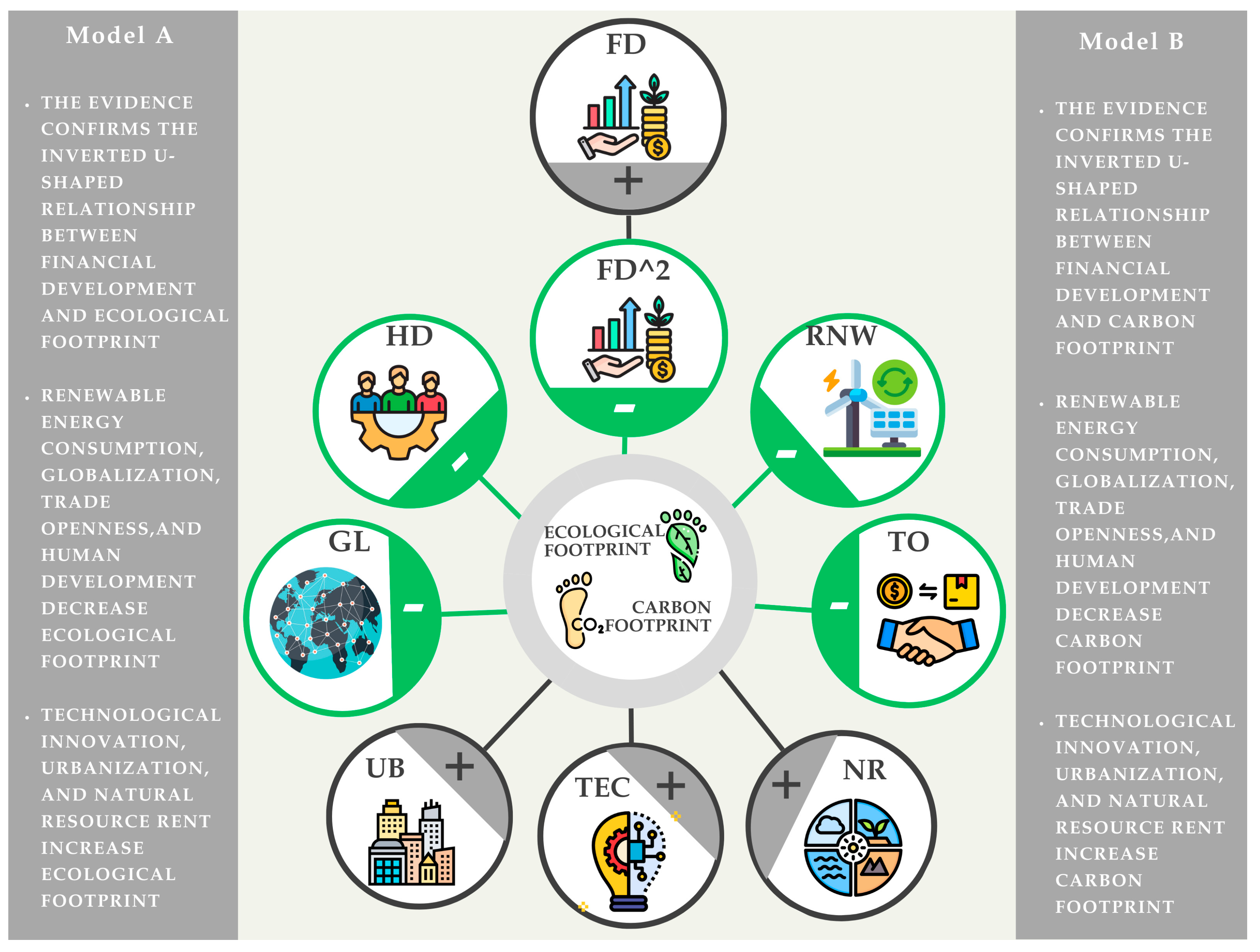
| Inverted U-shaped | Inverted U-shaped | Inverted U-shaped | Inverted U-shaped | |||||
| Adj. R2 | 0.892 *** | 0.861 *** | 0.947 *** | 0.981 *** | ||||
| Jarque Bera | 3.555 (0.168) | 0.403 (0.817) | 2.180 (0.336) | 0.569 (0.752) | ||||
| Ramsey’s Reset | 0.921 (0.357) | 1.047 (0.295) | 1.384 (0.138) | 1.681 (0.118) | ||||
| LM | 1.443 (0.124) | 1.568 (0.114) | 1.541 (0.118) | 1.583 (0.109) | ||||
| BPG | 1.820 (0.178) | 1.404 (0.216) | 1.536 (0.184) | 1.349 (0.260) | ||||
| Regressor | M-estimation | S-estimation | ||||||
| Model A 1 | Model B 2 | Model A 1 | Model B 2 | |||||
| coef. | prob. | coef. | prob. | coef. | prob. | coef. | prob. | |
| FD | 0.338 | 0.000 | 1.195 | 0.000 | 0.552 | 0.000 | 1.540 | 0.000 |
| FD^2 | −0.063 | 0.003 | −0.304 | 0.000 | −0.673 | 0.000 | −0.827 | 0.000 |
| NR | 0.076 | 0.000 | 0.061 | 0.000 | 0.005 | 0.000 | 0.068 | 0.000 |
| HD | −1.543 | 0.000 | −1.785 | 0.000 | −1.359 | 0.000 | −2.607 | 0.000 |
| TECt-1 | 0.010 | 0.000 | 0.062 | 0.000 | 0.041 | 0.004 | 0.047 | 0.005 |
| RNW | −0.015 | 0.000 | −0.050 | 0.000 | −0.048 | 0.000 | −0.088 | 0.000 |
| TO | −0.140 | 0.000 | −0.317 | 0.000 | −0.075 | 0.000 | −0.182 | 0.003 |
| UB | 0.910 | 0.000 | 0.943 | 0.000 | 0.445 | 0.000 | 1.595 | 0.000 |
| GL | −0.707 | 0.000 | −1.285 | 0.000 | −0.058 | 0.000 | −0.863 | 0.000 |
| Inverted U-shaped | Inverted U-shaped | Inverted U-shaped | Inverted U-shaped | |||||
| Adj. R2 | 0.433 *** | 0.427 *** | 0.457 *** | 0.208 *** | ||||
| Jarque Bera | 4.352 (0.113) | 0.136 (0.934) | 2.777 (0.249) | 2.871 (0.237) | ||||
| Ramsey’s Reset | 1.272 (0.203) | 1.434 (0.165) | 1.231 (0.293) | 1.448 (0.152) | ||||
| LM | 1.420 (0.159) | 1.982 (0.143) | 1.143 (0.333) | 1.953 (0.154) | ||||
| BPG | 2.360 (0.122) | 2.104 (0.125) | 1.735 (0.177) | 2.647 (0.104) | ||||
| Causality | Panel Fisher Stat. | Asymptotic Prob. | ||
|---|---|---|---|---|
| FD | → | EF | 76.666 | 0.000 |
| NR | → | EF | 66.190 | 0.000 |
| HD | → | EF | 68.364 | 0.000 |
| TEC | → | EF | 48.663 | 0.001 |
| RNW | → | EF | 96.092 | 0.000 |
| TO | → | EF | 73.093 | 0.000 |
| UB | → | EF | 66.983 | 0.000 |
| GL | → | EF | 59.021 | 0.000 |
| FD | → | CF | 76.474 | 0.000 |
| NR | → | CF | 81.927 | 0.000 |
| HD | → | CF | 57.663 | 0.000 |
| TEC | → | CF | 52.202 | 0.000 |
| RNW | → | CF | 112.271 | 0.000 |
| TO | → | CF | 75.349 | 0.000 |
| UB | → | CF | 83.233 | 0.000 |
| GL | → | CF | 52.757 | 0.000 |
| Causality | Panel Fisher Stat. | Asymptotic Prob. | Causality | Panel Fisher Stat. | Asymptotic Prob. | ||||
|---|---|---|---|---|---|---|---|---|---|
| FD+ | → | EF+ | 86.570 | 0.000 | FD+ | → | CF+ | 168.249 | 0.000 |
| FD+ | → | EF− | 81.270 | 0.000 | FD+ | → | CF− | 83.442 | 0.000 |
| FD− | → | EF− | 63.022 | 0.000 | FD− | → | CF− | 110.736 | 0.000 |
| FD− | → | EF+ | 39.905 | 0.011 | FD− | → | CF+ | 64.087 | 0.000 |
| NR+ | → | EF+ | 37.609 | 0.020 | NR+ | → | CF+ | 280.565 | 0.000 |
| NR+ | → | EF− | 62.587 | 0.000 | NR+ | → | CF− | 48.677 | 0.001 |
| NR− | → | EF− | 47.886 | 0.001 | NR− | → | CF− | 106.533 | 0.000 |
| NR− | → | EF+ | 150.303 | 0.000 | NR− | → | CF+ | 94.083 | 0.000 |
| HD+ | → | EF+ | 81.905 | 0.000 | HD+ | → | CF+ | 65.271 | 0.000 |
| HD+ | → | EF− | 42.149 | 0.003 | HD+ | → | CF− | 50.499 | 0.000 |
| HD− | → | EF− | 14.059 | 0.827 | HD− | → | CF− | 251.103 | 0.000 |
| HD− | → | EF+ | 176.458 | 0.000 | HD− | → | CF+ | 130.227 | 0.000 |
| TEC+ | → | EF+ | 84.038 | 0.000 | TEC+ | → | CF+ | 92.336 | 0.000 |
| TEC+ | → | EF− | 109.041 | 0.000 | TEC+ | → | CF− | 54.675 | 0.000 |
| TEC− | → | EF− | 78.086 | 0.000 | TEC− | → | CF− | 68.994 | 0.000 |
| TEC− | → | EF+ | 29.169 | 0.140 | TEC− | → | CF+ | 18.080 | 0.701 |
| RNW+ | → | EF+ | 59.884 | 0.000 | RNW+ | → | CF+ | 86.185 | 0.000 |
| RNW+ | → | EF− | 95.369 | 0.000 | RNW+ | → | CF− | 60.048 | 0.000 |
| RNW− | → | EF− | 50.736 | 0.000 | RNW− | → | CF− | 62.146 | 0.000 |
| RNW− | → | EF+ | 21.164 | 0.388 | RNW− | → | CF+ | 22.542 | 0.312 |
| TO+ | → | EF+ | 45.632 | 0.002 | TO+ | → | CF+ | 46.283 | 0.000 |
| TO+ | → | EF− | 142.617 | 0.000 | TO+ | → | CF− | 77.094 | 0.000 |
| TO− | → | EF− | 34.459 | 0.044 | TO− | → | CF− | 176.040 | 0.000 |
| TO− | → | EF+ | 90.522 | 0.000 | TO− | → | CF+ | 66.133 | 0.000 |
| UB+ | → | EF+ | 57.493 | 0.000 | UB+ | → | CF+ | 91.620 | 0.000 |
| UB+ | → | EF− | 96.569 | 0.000 | UB+ | → | CF− | 80.180 | 0.000 |
| UB− | → | EF− | 149.198 | 0.000 | UB− | → | CF− | 146.812 | 0.000 |
| UB− | → | EF+ | 47.123 | 0.001 | UB− | → | CF+ | 190.579 | 0.000 |
| GL+ | → | EF+ | 140.591 | 0.000 | GL+ | → | CF+ | 144.062 | 0.000 |
| GL+ | → | EF− | 67.021 | 0.000 | GL+ | → | CF− | 79.336 | 0.000 |
| GL− | → | EF− | 20.905 | 0.527 | GL− | → | CF− | 71.274 | 0.000 |
| GL− | → | EF+ | 38.905 | 0.014 | GL− | → | CF+ | 11.476 | 0.967 |
Disclaimer/Publisher’s Note: The statements, opinions and data contained in all publications are solely those of the individual author(s) and contributor(s) and not of MDPI and/or the editor(s). MDPI and/or the editor(s) disclaim responsibility for any injury to people or property resulting from any ideas, methods, instructions or products referred to in the content. |
© 2025 by the authors. Licensee MDPI, Basel, Switzerland. This article is an open access article distributed under the terms and conditions of the Creative Commons Attribution (CC BY) license (https://creativecommons.org/licenses/by/4.0/).
Share and Cite
Topaloglu, E.E.; Balsalobre-Lorente, D.; Nur, T.; Ege, I. The Relevance of Financial Development, Natural Resources, Technological Innovation, and Human Development for Carbon and Ecological Footprints: Fresh Evidence of the Resource Curse Hypothesis in G-10 Countries. Sustainability 2025, 17, 2487. https://doi.org/10.3390/su17062487
Topaloglu EE, Balsalobre-Lorente D, Nur T, Ege I. The Relevance of Financial Development, Natural Resources, Technological Innovation, and Human Development for Carbon and Ecological Footprints: Fresh Evidence of the Resource Curse Hypothesis in G-10 Countries. Sustainability. 2025; 17(6):2487. https://doi.org/10.3390/su17062487
Chicago/Turabian StyleTopaloglu, Emre E., Daniel Balsalobre-Lorente, Tugba Nur, and Ilhan Ege. 2025. "The Relevance of Financial Development, Natural Resources, Technological Innovation, and Human Development for Carbon and Ecological Footprints: Fresh Evidence of the Resource Curse Hypothesis in G-10 Countries" Sustainability 17, no. 6: 2487. https://doi.org/10.3390/su17062487
APA StyleTopaloglu, E. E., Balsalobre-Lorente, D., Nur, T., & Ege, I. (2025). The Relevance of Financial Development, Natural Resources, Technological Innovation, and Human Development for Carbon and Ecological Footprints: Fresh Evidence of the Resource Curse Hypothesis in G-10 Countries. Sustainability, 17(6), 2487. https://doi.org/10.3390/su17062487