A Hybrid Optimization Approach Combining Rolling Horizon with Deep-Learning-Embedded NSGA-II Algorithm for High-Speed Railway Train Rescheduling Under Interruption Conditions

Abstract

This study discusses the issue of train rescheduling in high-speed railways (HSR) when unexpected interruptions occur. These interruptions can lead to delays, cancellations, and disruptions to passenger travel. An optimization model for train rescheduling under uncertain-duration interruptions is proposed. The model aims to minimize both the decline in passenger service quality and the total operating cost, thereby achieving sustainable rescheduling. Then, a hybrid optimization algorithm combining rolling horizon optimization with a deep-learning-embedded NSGA-II algorithm is introduced to solve this multi-objective problem. This hybrid algorithm combines the advantages of each single algorithm, significantly improving computational efficiency and solution quality, particularly in large-scale scenarios. Furthermore, a case study on the Beijing–Shanghai high-speed railway shows the effectiveness of the model and algorithm. The optimization rates are 16.27% for service quality and 15.58% for operational costs in the small-scale experiment. Compared to other single algorithms or algorithm combinations, the hybrid algorithm enhances computational efficiency by 26.21%, 15.73%, and 25.13%. Comparative analysis shows that the hybrid algorithm outperforms traditional methods in both optimization quality and computational efficiency, contributing to enhanced overall operational efficiency of the railway system and optimized resource utilization. The Pareto front analysis provides decision makers with a range of scheduling alternatives, offering flexibility in balancing service quality and cost. In conclusion, the proposed approach is highly applicable in real-world railway operations, especially under complex and uncertain conditions, as it not only reduces operational costs but also aligns railway operations with broader sustainability goals.

1. Introduction

In recent decades, the high-speed railway (HSR) has increasingly become an indispensable means of transportation for passengers worldwide. The HSR is eco-friendly as its primary energy comes from electricity instead of oil, thus cutting down on carbon emissions and aiding in sustainable energy development and the achievement of a “low-carbon economy”. However, in the daily operation of high-speed railways, a series of unexpected events will inevitably occur, causing interruptions in train operations. These interruptions will result in different degrees of train delays and even train cancellations, thus affecting the travel of passengers and costing significant energy, which is not conducive to sustainable development.

In most cases, during the initial period when an interruption occurs, the dispatchers may not have access to all the detailed information about the interruption, making it difficult to assess the duration of the interruption accurately. Moreover, interruptions caused by unforeseen events inherently possess uncertainty, which makes accurate judgment of the duration even more challenging. If the dispatchers frequently issue train scheduling commands because of this, it will not only lead to the waste of transportation resources but also cause interference with the work of train scheduling, potentially causing a certain degree of safety hazard. Therefore, regarding the adjustment of the train timetable after unforeseen events, this paper considers the situation where the duration of the interruption is uncertain for the dispatchers. The rolling horizon approach is applied in the train operation adjustment process to handle the interruption’s uncertain duration. The objective is to minimize the decline of passenger service quality and total operation cost as much as possible, ultimately obtaining a train operation plan under uncertain interruption durations.

Figure 1 depicts an example of a small-scale high-speed railway timetable. The timetable consists of six stations, five sections, and six trains. The horizontal axis represents time, while the vertical axis represents distance. Due to an unexpected event, one-way operation is interrupted in section 3 of Figure 1, and trains cannot pass through the section. Consequently, trains G1 and G3 are halted at Station 3, waiting until the interruption ceases. These trains are referred to as interrupted trains. The dashed lines in Figure 1 represent the original planned routes of these trains. We call the delayed passenger flow due to interruption “affected passenger flow” and call the delayed trains due to interruption “affected trains”.

After the interruption, considering the affected passenger flow, a series of measures including changing train sequences in the sections and adjusting train stops are applied to minimize the decline in passenger service quality. To balance the increase in train operating costs that may arise from improving passenger service quality, we introduce a second objective function to minimize train operating costs, to seek a balance between the two objective functions, and provide railway operators with diverse solutions containing different objective function values to satisfy their different tendencies and needs.

We can see from Figure 1, train G1 and train G3 cannot pass through section 2 on time due to the interruption. After the interruption, the running order of trains G1 and G3 has been adjusted without significantly impacting the operation schedules of trains G5, G7, G9, and G11. The running order in section 3 changes from G1-G3-G5-G7-G9-G11 to G5-G1-G7-G9-G3-G11. Accordingly, the stopping times of train G1 at Station 5 and train G3 at Station 4 are extended for some time to meet the time interval at the station. In this situation, although the stopping time of trains G1 and G3 at the station has increased, it has avoided longer delays or even cancellations caused by the overall delay of the train running line. Additionally, the passenger flow with origin–destination (OD) from Station 3 to Station 6 on trains G1 and G3 can also be served by train G5, provided that train G5 has sufficient remaining passenger capacity. This can significantly reduce the delay for this portion of the passenger flow without changing the train timetable and resulting in more operation costs.

In this paper, we intend to establish a train timetable adjustment model under interruption conditions to describe the problem. We use a rolling horizon approach to handle the problem of uncertain interruption duration and finally use a hybrid algorithm embedded in a deep learning algorithm to solve the model.

2. Literature Review

High-speed railway (HSR) train scheduling and timetable adjustment are key to ensuring efficient and reliable railway operations. Early studies focused on resolving scheduling conflicts and improving the utilization of railway infrastructure. For more efficiently resolving resource conflicts in train traffic rescheduling, Yu [1] proposed a hybrid method of network-based simulation and event-driven simulation. This method combines the advantages of two simulation methods and verifies the impact of the proposed method on overall performance through simple examples. The experimental results show that this method can effectively solve the problem of resource conflicts in train scheduling. Sahin [2] analyzed the decision-making process of dispatchers in resolving conflicts between trains and developed a heuristic algorithm that considers the impact of potential conflicts. By modifying the existing train operation plan in the event of a single-line railway conflict, the system’s total delay caused by conflicting train shutdowns was reduced. Subsequent research expanded on this to concentrate on timetable stability, passenger service quality, and the management of delays. Norio et al. [3] proposed a train scheduling algorithm and treated the train rescheduling problem as a constrained optimization problem, with the optimization objective of minimizing passenger dissatisfaction. Feasibility was verified using actual operational data. Yang et al. [4] established a two-stage fuzzy optimization model intended to minimize the total delay time of the rearranged train schedule to obtain a robust rescheduling plan under suddenly unstable conditions. Numerical experiments have demonstrated the effectiveness of the proposed method. In recent years, the focus has shifted to addressing the increasingly complex large-scale issues in high-speed railway operations, especially in situations of uncertainty and interruption. Cavone et al. [5] proposed a self-learning decision-making process for train rescheduling on railway networks under interference conditions. The quality of rescheduling is improved every time the method is reapplied. This technology was applied to a real dataset related to the railway network in southern Italy to test its effectiveness. Zhou et al. [6] studied the coordinated rescheduling problem of multiple scheduling sections of high-speed railways under large-scale interruptions from a macro perspective and formulated it as a mixed integer linear programming (MILP) model, to minimize the weighted sum of the total delay time and the number of train delays. Subsequently, a case study was conducted using the Beijing–Shanghai high-speed railway as an example to evaluate the performance of the proposed comprehensive rescheduling method. Sun et al. [7] proposed a collaborative adjustment model for train timetables on the railway network, with the optimization objectives of reducing total passenger waiting time and penalty time caused by exceeding train capacity, which was solved by the genetic algorithm.

The methodologies for the study of train scheduling can currently be divided into three categories: research methods based on simulation, research methods based on operations research methods, and research methods based on artificial intelligence.

Nie Lei et al. [8] established a model based on the arrival and departure sequence of trains, used computer simulation methods, used four adjustment strategies, and conducted simulation experiments under eight different train operation interferences. They compared and analyzed the relationship between medium- and high-speed trains and their impact on train operation adjustments.

Jones et al. [9] proposed a hybrid simulation method that combines heuristics to determine train schedules and destination stations in a mining freight railway network. This method combines discrete event simulation with agent-based modeling and heuristics and combines the set of simulated operations to control the selection of train destination stations. Högdahl et al. [10] proposed a combined simulation optimization method for double-track railways and established a new and more universal model to predict delays, allowing for flexible adjustment of train sequences. This method weights the minimum total train operation time and total predicted delay to optimize the given train timetable. Simulation experiments were conducted on the severely congested western trunk line in Sweden, demonstrating the effectiveness of the method.

Operational research methods are currently the predominant approach for optimizing train timetables. Firstly, based on the objectives and characteristics of the problem, an integer programming model or mixed-integer programming model is established. Then, classical operations research methods (branch and bound method [11], Lagrange algorithm [12], dynamic programming algorithm [13], ADMM algorithm [14]) or heuristic algorithms (genetic algorithm [15], simulated annealing algorithm [16], ant colony algorithm [17], particle swarm algorithm [18]) are selected for solution.

In recent years, artificial intelligence has developed rapidly and is widely used in various areas of transportation, such as urban rail transit [19] and road traffic [20]. Moreover, the combination of artificial intelligence and train timetable adjustment has also become a hot topic. Ning et al. [21] introduced a deep reinforcement learning (DRL) method to minimize the average delay time of all trains. They used block sections and stations to establish a state set, a learning environment set, and a reward function. Then, they used the learning agent to continuously learn and adjust the sequence, running time, dwell time, and departure time of the trains to obtain the final train timetable. The experiment was tested on the Beijing–Shanghai high-speed railway and proved that, compared with the first come, first serve (FCFS) method, this method can reduce the average delay time by 46.38%. Li and Ni [22] proposed a multi-agent deep reinforcement learning method for train scheduling. The method constructs a general train scheduling learning environment and models the problem as a Markov decision process. To solve multi-dimensional problems, a multi-agent actor-critic algorithm framework is proposed. This framework can decompose a large combined decision space into multiple independent decision spaces and parameterize it through deep neural networks. Sun et al. [23] proposed three models for the optimization and adjustment of a train timetable under dynamic passenger flow demand to minimize the average waiting time of passengers. Then, they evaluated the performance of the three models and conducted sensitivity analysis on different parameters of Singapore subway lines. Zhang et al. [24] proposed a multi-step passenger flow prediction model based on deep learning, called EF former, which is an abbreviation for event flow transformer network, to address the complex temporal evolution characteristics of urban rail transit passenger flow during large-scale events. In the process of training deep learning models, appropriate techniques should be employed to enhance accuracy and prevent overfitting. In terms of dataset processing, Verónica et al. [25] conducted experimental evaluations on several popular datasets using well-known feature selection methods, providing a comparative study for the research community. Regarding the reduction of dataset complexity, Hossein et al. [26] used a hold-out set for training–validation splits instead of computationally expensive k-fold cross-validation. This approach simplifies the training process while still providing a reliable estimate of model performance. The use of dropout regularization (rate of 0.2) and ReLU activation functions also helps prevent overfitting, contributing to a more robust and accurate model without increasing complexity.

For the interference duration in train operation adjustment, many scholars simplify it to a fixed duration to reduce the complexity of the problem and obtain a high-quality train operation adjustment plan. Özgür et al. [27] set fixed durations for track failures and used a stochastic simulation-based train timetable generation framework to reschedule the train timetable for efficiency. Liao [28] set up multiple groups of fixed-duration interruptions for two scenarios: the origin station is unable to send out trains due to unexpected events and a two-direction interruption in the section due to unexpected events. Based on the fireworks algorithm, he analyzed the solution efficiency and quality for interruptions with different durations. Focused on interruptions during train operations and the recovery of operation order after the interruption, Konstantinos et al. [29] and Krasemann [30] defined interruption as a scenario where one or more train schedules deviate from the planned timetable due to certain factors. However, different solving methods were used. Krasemann used heuristic algorithms to solve the problem, while Konstantinos et al. proposed a model that can efficiently deal with train operation interference and provided an easy-to-solve mathematical method to obtain the global optimal solution. Shakibayifar et al. [31] proposed a model for adjusting the train timetable on Iran’s railway network in response to interruptions during daily operations, aiming to resolve conflicts between trains by changing their passing sequence. They developed a two-stage heuristic algorithm to solve the model and tested it on an actual rail network, discussing its strengths and limitations.

Additionally, some researchers have explored interruptions with uncertain durations, most of whom adopt rolling optimization strategies for analysis. Zhan et al. [32] adjusted train passing sequences and arrival/departure times for two-direction interruptions on double-track railways. They used rolling optimization strategies to optimize train schedules under uncertain disruption durations and validated the method through an example on the Beijing–Shanghai high-speed railway. Törnquist [33], Peng et al. [34], Pellegrini et al. [35], and Zhu et al. [36] all utilized rolling optimization strategies to study train operation adjustment problems with positive results. Samà et al. [37] applied rolling optimization strategies to optimize aircraft scheduling plans in the context of airport scheduling issues.

We can see the following through the above papers:

• Train timetable adjustment methods can be categorized into simulation-based, operations-research-based, and artificial-intelligence-based approaches. Simulation and optimization research techniques, such as mixed-integer programming and heuristic algorithms, have been widely used to adjust train schedules and minimize delays. More recently, deep reinforcement learning (DRL) has shown potential for optimizing timetables in real time, outperforming traditional methods in terms of reducing delays. However, few researchers concentrate on the integration between deep learning techniques and heuristic algorithms, which may further enhance optimization efficiency.
• Handling interference in train schedules involves both fixed-duration and uncertain-duration approaches. Fixed-duration models simplify interruption scenarios, allowing for efficient rescheduling. For unpredictable disruptions, rolling optimization strategies are widely used to adjust schedules dynamically in real time. These methods have proven effective in reducing delays and restoring operational order, especially under complex and busy conditions, and are also being applied in other transportation systems.

The main contributions of the paper are as follows:

• Hybrid optimization algorithm integrating deep learning: This paper proposes a hybrid optimization algorithm that combines rolling horizon optimization with a deep-learning-embedded NSGA-II algorithm. This approach leverages deep learning to model the uncertainty in train operation adjustments and integrates the advantages of the NSGA-II algorithm, effectively solving multi-objective optimization problems. This innovative algorithm design better addresses the complexities and uncertainties of high-speed rail operation, improving decision quality and efficiency in train schedule adjustments.
• Fast computational speed, particularly for large-scale cases, requiring less resource consumption and making transportation greener and more sustainable: Traditional rolling horizon optimization algorithms have limitations when handling large-scale complex problems. To overcome this shortcoming, this paper uses a deep-learning-embedded NSGA-II algorithm to solve the train operation scheduling problem. Deep learning, by learning from large amounts of historical data, can predict potential delays and disruptions, thus optimizing the decision-making process. The integration of the NSGA-II algorithm’s multi-objective optimization capability enables faster solution times while handling large-scale complex problems, significantly improving the performance of rolling horizon optimization, particularly in real-world scenarios with large-scale and high-complexity problems. This measure can use less resources in the process of the calculation and reduce emissions indirectly, which contributes to low-carbon and sustainable transportation.
• The application of the NSGA-II algorithm provides decision makers with different choices: The paper employs the non-dominated sorting genetic algorithm II (NSGA-II) to solve the multi-objective optimization problem and generate a set of Pareto-optimal solutions. This approach allows decision makers to choose from a range of feasible alternatives, balancing multiple conflicting objectives, such as minimizing passenger service degradation and operational costs. The NSGA-II algorithm’s ability to produce a diverse set of solutions, each representing a trade-off between the objectives, provides decision makers with valuable insights into the potential outcomes of different scheduling strategies. This flexibility is particularly important in scenarios where decision makers need to consider multiple objectives simultaneously and make informed choices based on real-time, uncertain conditions.

3. Model

In this section, we establish a mixed-integer programming model to solve the problem of optimizing and adjusting train schedules under uncertain interruption times. In Section 3.1, we start by explaining the symbols and parameters we use in the model, including sets, symbols, and decision variables. Thereafter, in Section 3.2, we introduce the assumptions we use in this paper. Finally, in Section 3.3, we introduce the objectives and constraints of the model.

3.1. Model Description

Table 1. Sets.

Symbol	Definition
$T$	The set of trains in the train timetable, indexed with $t_1$ and $t_2$
$T_{\mathrm{aff}}$	The set of affected trains, $T_{\mathrm{aff}}\subset T$
$J$	The set of stations, indexed with $j_1$ and $j_2$
$X$	The set of passenger demands
$X_{\mathrm{aff}}$	The set of affected passenger demands
$E$	The set of sections, indexed with $e_1$ and $e_2$—if the stations at both ends of the interval are $j$ and $j+1$, respectively, then the interval can be represented as $e=j,j+1$
$\Theta$	The set of rolling step $\varpi$

,

Table 2. Parameters.

Parameters	Definition
$T_{\mathrm{start}}$	The start time of the period for solving the timetable
$T_{\mathrm{end}}$	The end time of the period for solving the timetable
$T_{\mathrm{pd}}^{t,j}$	The scheduled departure time of train $t$ at station $j$
$T_{\mathrm{pa}}^{t,j}$	The scheduled arrival time of train $t$ at station $j$
$S_{\mathrm{end}}^t$	The end station of train $t$
$S_{\mathrm{start}}^t$	The start station of train $t$
$S_{\mathrm{end}}^{t,x}$	The end station of passenger flow $x$ in train $t$
$S_{\mathrm{start}}^{t,x}$	The start station of passenger flow $x$ in train $t$
$T_{\mathrm{can}}^{\mathrm{pas}}$	Penalty value for the cancellation of a passenger flow
$T_{\mathrm{start}}^{\mathrm{itr}}$	The start time of the interruption
$T_{\mathrm{predur}}^{\varpi }$	The predicted interruption duration in rolling step $\varpi$
$T_{\mathrm{begin}}^{\varpi }$	The start time of rolling step $\varpi$, $\varpi =1,2,\dots ,\mathrm{m}$; m is the number of rolling steps
$T_{\mathrm{end}}^{\varpi }$	The end time of rolling step $\varpi$, $\varpi =1,2,\dots ,\mathrm{m}$; m is the number of rolling steps
$E_{\mathrm{occur}}^{\mathrm{itr}}$	The section where the interruption occurs
$S_{\mathrm{start}}^{\mathrm{itr}}$	The start station of the section where the interruption occurs
$S_{\mathrm{end}}^{\mathrm{itr}}$	The end station of the section where the interruption occurs
$T_{\mathrm{lat}}^{t,x,j}$	The latest arrival time of passenger flow $x$ at station $j$
$T_{\mathrm{stop}}^j$	The stop time of the train at station $j$
$T_{\mathrm{exs}}^j$	The extra starting time of the train at station $j$
$T_{\mathrm{exd}}^j$	The extra stopping time of the train at station $j$
$T_{\mathrm{run}}^{j,j+1}$	The running time of train $t$ in section $j,j+1$
$D_{\mathrm{btw}}^{j,j+1}$	The distance of the section $j,j+1$
$C_{\mathrm{oper}}^{\mathrm{train}}$	The operation cost per kilometer for each train
$C_{\mathrm{oper}}^{\mathrm{pas}}$	The cost per kilometer for each passenger
$T_{\mathrm{amd}}$	The maximum allowable additional dwell time
$T_{btt}$	The time interval between two consecutive trains passing through the same station.
$W_{\mathrm{stop}}^{t,j}$	Whether train $t$ is scheduled to stop at station $s$—if it stops, the value is 1; otherwise, the value is 0
$W_{\mathrm{pass}}^{t,j,j+1}$	Whether train $t$ passes through section $j,j+1$—if train $t$ passes through section $j,j+1$, its value is 1; otherwise, its value is 0
$N_{\mathrm{pp}}^t$	The planned number of passengers in train $t$
$N_{\mathrm{pas}}^{t,x}$	The number of passengers in passenger flow $x$ in train $t$
$N_{\mathrm{cap}}^t$	The passenger carrying capacity of train $t$
$c_1,c_2$	The coefficients inside objective function 1
$M$	A real number that is large enough

, and

Table 3. Decision variables.

Symbol	Definition
${\theta }_j^t$	The actual departure time of train $t$ in station $j$
${\tau }_j^t$	The actual arrival time of train $t$ in station $j$
${\delta }^t$	0–1 variable, whether train $t$ is cancelled—if train $t$ is cancelled, its value is 1; otherwise, its value is 0
${\delta }^{t,x}$	0–1 variable, whether passenger flow $x$ in train $t$ is cancelled—if passenger flow $x$ in train $t$ is cancelled, its value is 1; otherwise, its value is 0
${\psi }_t^e$	The sequence in which train $t$ passes through section $e$, ${\psi }_t^e$ = 1, 2, …, K, where K is the total number of trains
${\epsilon }_j^t$	0–1 variable, whether train $t$ stops at station $j$—if train $t$ stops at station $j$, its value is 1; otherwise, its value is 0
${\eta }_{j,j+1}^{t,t\text{'}}$	0–1 variable, the order in which train $t$ and train $t\text{'}$ pass through the section $j,j+1$—if train $t$ passes through the section before train $t\text{'}$, its value is 1; otherwise, its value is 0
${\sigma }_{t\text{'}}^{t,x}$	The number of affected passenger flow $x$ in train $t$ served by train $t\text{'}$
${\mu }_{t\text{'}}^{t,x}$	0–1 variable, whether the passenger flow $x$ on train $t$ is served by train $t\text{'}$—if the passenger flow $x$ on train $t$ is served by train $t\text{'}$, its value is 1; otherwise, its value is 0

present the sets, decision variables, and parameters used in this paper, respectively.

3.2. Model Assumptions

• All trains adjust their passing sequence and station stop plans without changing the length of the original train operation lines.
• Prior to the occurrence of disruptions, all trains operate according to the scheduled train timetable.
• After adjustments to their passing sequence and stop plans, the trains or passenger flows that still fail to meet the constraints will be canceled.

3.3. Model Formulation

We have set two objective functions, which are the minimum decline in passenger service quality and the minimum total operating cost:

(1)

Minimum decline in passenger service quality

The passenger service quality is a critical metric in evaluating the performance and efficiency of transportation. After the interruption occurs, we should try to minimize the decline in passenger service quality, which encompasses two distinct components. The first and most important component is the quality decline of the cancelled passengers due to the adjustment of the trains. The second component is the quality decline of the passenger delay. This includes passengers who have boarded the train and are experiencing delays due to operational issues, such as technical problems, weather conditions, or scheduling conflicts. Considering that the cancellation of passenger flow has a greater impact on the quality of passenger service than the delay of passengers, we have set weight coefficients $c_1$ and $c_2$ for these two parts, where $c_1$ is greater than $c_2$.

Both types of passenger service quality decline contribute to the overall impact on the transportation system’s reliability and passengers’ satisfaction. Railway operators need to monitor and manage these problems to minimize their effects on passengers and to maintain a high level of service quality.

$$Z_1=\min c_1{\displaystyle \sum _{t\in T}{\displaystyle \sum _{x\in X}({\delta }^{t,x}\times T_{\mathrm{can}}^{\mathrm{pas}}\times N_{\mathrm{pas}}^{t,x})}}+c_2{\displaystyle \sum _{t\in T}({\tau }_{S_{\mathrm{end}}^t}^t-T_{\mathrm{pa}}^{t,S_{\mathrm{end}}^t})\times (N_{\mathrm{pp}}^t+{\displaystyle \sum _{t\text{'}\in T_{\mathrm{aff}}}{\displaystyle \sum _{x\in X}{\sigma }_t^{t\text{'},x}}})}$$

(1)

(2)

Minimum total operating cost

The total operating cost consists of two main components: one is the train operation distance cost, which is directly related to the train’s operating distance and includes fuel consumption, vehicle wear and tear, track maintenance, etc.; the other is the passenger service cost, which is related to the number of passengers, such as passenger services, cleaning, laundry, etc. These two parts of the cost jointly determine the total operating cost of the train.

$$Z_2=\min {\displaystyle \sum _{t\in T}{\displaystyle \sum _{j=S_{\mathrm{start}}^t}^{S_{\mathrm{end}}^t}{D}_{\mathrm{btw}}^{j,j+1}\times C_{\mathrm{oper}}^{\mathrm{train}}\times (1-{\delta }^t)}}+{\displaystyle \sum _{t\in T}{\displaystyle \sum _{x\in X}{\displaystyle \sum _{j=S_{start}^{t,x}}^{S_{end}^{t,x}}{N}_{\mathrm{pas}}^{t,x}\times C_{\mathrm{oper}}^{\mathrm{pas}}\times D_{\mathrm{btw}}^{j,j+1}\times (1-{\delta }^{t,x})}}}$$

(2)

3.4. Constraints

The following are the constraints of the model:

(1)

Constraints of time range

The arrival and departure time of the train should be within the required time range of train operation. The operation schedule commences at 6:00 and concludes at 24:00, where 360 and 1440, denoted in minutes, correspond to 6:00 and 24:00, respectively.

$$360\le {\tau }_j^t\le 1440,\forall t\in T,j\in J$$

(3)

$$360\le {\theta }_j^t\le 1440,\forall t\in T,j\in J$$

(4)

Similarly, during each rolling solution period, the arrival and departure time of the train cannot exceed the time range of the solving period.

$$T_{\mathrm{begin}}^{\varpi }\le {\tau }_j^t\le T_{\mathrm{end}}^{\varpi },\forall t\in T_{\varpi },j\in J,\varpi \in \Theta$$

(5)

$$T_{\mathrm{begin}}^{\varpi }\le {\theta }_j^t\le T_{\mathrm{end}}^{\varpi },\forall t\in T_{\varpi },\varpi \in \Theta$$

(6)

(2)

Constraints of station stop time

The actual dwell time of the train in station $j$ must be greater than or equal to the required dwell time $T_{\mathrm{stop}}^j$ and cannot exceed the required dwell time plus the maximum allowable additional dwell time $T_{\mathrm{amd}}$:

$${\theta }_j^t-{\tau }_j^t\le {\epsilon }_j^t\times W_{\mathrm{stop}}^{t,j}\times (T_{\mathrm{stop}}^j+T_{\mathrm{amd}}),\forall t\in T,j\in J$$

(7)

$${\theta }_j^t-{\tau }_j^t\ge {\epsilon }_j^t\times W_{\mathrm{stop}}^{t,j}\times T_{\mathrm{stop}}^j,\forall t\in T,j\in J$$

(8)

(3)

Constraint of station tracking interval

The arrival and departure times of adjacent trains at the station must meet the station tracking interval, that is, the actual time interval between two consecutive trains passing through the same station must be greater than or equal to $T_{btt}$.

$${\tau }_j^{t\text{'}}-{\tau }_j^t+(1-{\eta }_{j,j+1}^{t,t\text{'}})\times M\ge T_{btt},\forall t,t\text{'}\in T,j,j+1\in J$$

(9)

$${\theta }_j^{t\text{'}}-{\theta }_j^t+(1-{\eta }_{j,j+1}^{t,t\text{'}})\times M\ge T_{btt},\forall t,t\text{'}\in T,j,j+1\in J$$

(10)

(4)

Constraints of train operation time

To ensure the quality of train service, the arrival time of the train at the station shall not be earlier than the scheduled arrival time:

$${\theta }_j^t\ge T_{\mathrm{pa}}^{t,j}\times W_{\mathrm{stop}}^{t,j},\forall t\in T,j\in J$$

(11)

Similarly, the departure time of the train from the station shall not be earlier than the scheduled departure time of the train at the station:

$${\tau }_j^t\times W_{\mathrm{stop}}^{t,j}\le T_{\mathrm{pd}}^{t,j},\forall t\in T,j\in J$$

(12)

In the section where the interruption occurs, trains must depart after the interruption has been solved, that is, the departure time of the train should be later than the end time of the interruption, as shown in constraint (6):

$${\theta }_j^t\ge T_{\mathrm{start}}^{\mathrm{itr}}+T_{\mathrm{predur}}^{\varpi },\forall t\in T,j=S_{\mathrm{start}}^{\mathrm{itr}},\varpi \in \Theta$$

(13)

(5)

Allocation constraints of passenger flow

The passenger flow of the interrupted train is served by the affected train and must meet the following constraints:

The remaining passenger capacity of the train should be greater than or equal to the total number of affected passenger flows served by the train:

$${\displaystyle \sum _{x\in X}{\sigma }_{t\text{'}}^{t,x}}\le N_{\mathrm{cap}}^{t\text{'}}-N_{\mathrm{pp}}^{t\text{'}},\forall t\in T_{\mathrm{aff}},t\text{'}\in T,x\in X$$

(14)

If a train serves an affected passenger flow, it must stop at the start station and the end station of that passenger flow:

$${\displaystyle \frac{{\sigma }_{t\text{'}}^{t,x}}{{\sigma }_{t\text{'}}^{t,x}+1}}\le {\epsilon }_{S_{start}^{t\text{'},x}}^{t\text{'}},\forall t\in T_{\mathrm{aff}},t\text{'}\in T,x\in X$$

(15)

$${\displaystyle \frac{{\sigma }_{t\text{'}}^{t,x}}{{\sigma }_{t\text{'}}^{t,x}+1}}\le {\epsilon }_{S_{end}^{t\text{'},x}}^{t\text{'}},\forall t\in T_{\mathrm{aff}},t\text{'}\in T,x\in X$$

(16)

The number of passengers served by a train for a certain passenger flow cannot exceed the total number of passengers in that passenger flow:

$${\displaystyle \sum _{x\in X}{\sigma }_{t\text{'}}^{t,x}}\le N_{\mathrm{pas}}^{t,x},\forall t\in T_{\mathrm{aff}},t\text{'}\in T,x\in X$$

(17)

The number of passengers is an integer:

$${\sigma }_{t\text{'}}^{t,x}\in Z,\forall t\in T_{\mathrm{aff}},t\text{'}\in T,x\in X$$

(18)

(6)

Train overtaking constraint

It is stipulated that each train can only be overtaken by one train at a time, and each train can only be overtaken by one train at the same time:

$${\psi }_t^{e_m}-{\psi }_t^{e_{m+1}}\ge -1,\forall t\in T,e_m,e_{m+1}\in E$$

(19)

$${\psi }_t^{e_m}-{\psi }_t^{e_{m+1}}\le 1,\forall t\in T,e_m,e_{m+1}\in E$$

(20)

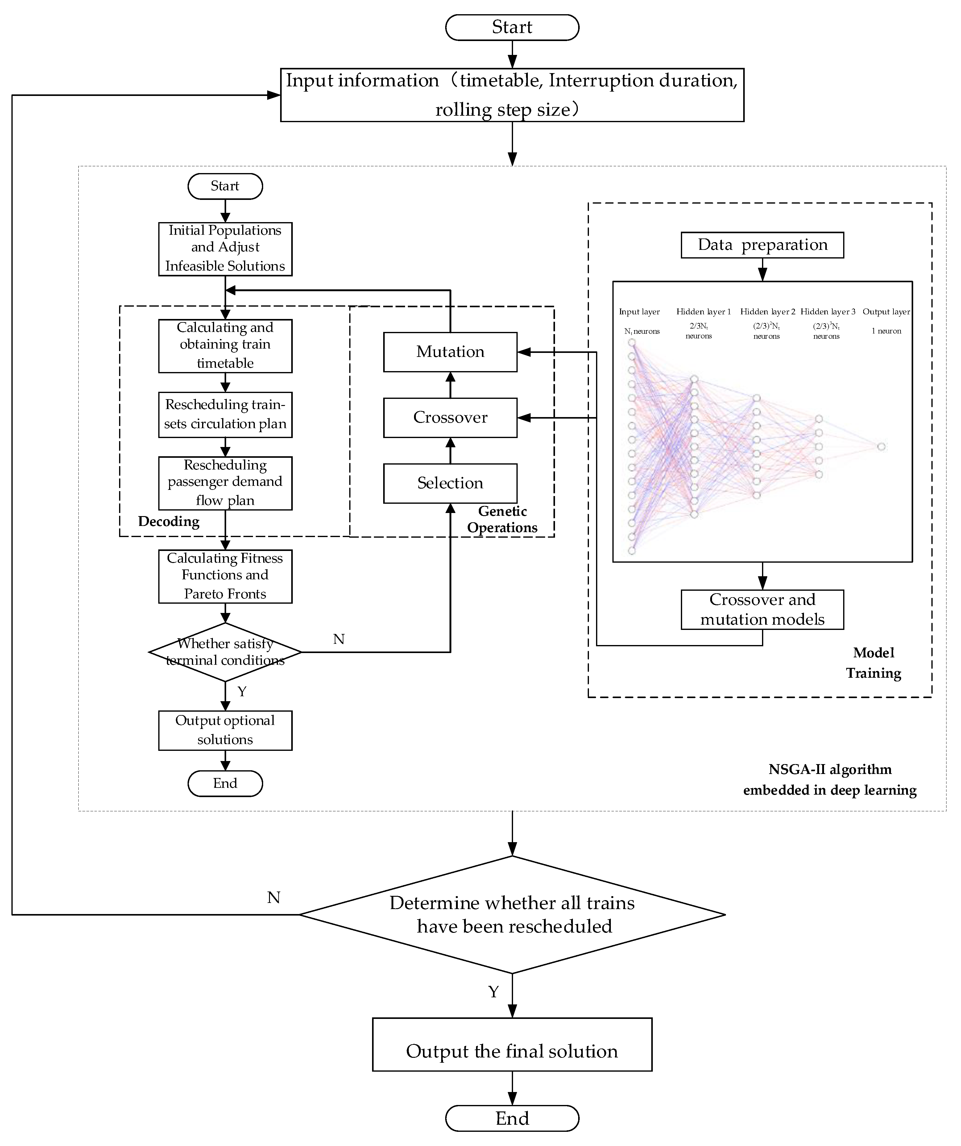
4. A Hybrid Solving Algorithm for the Rescheduling Problem

This section introduces a hybrid optimization algorithm for high-speed railway train operation adjustment. The algorithm uses a rolling horizon algorithm to handle the uncertain duration of interruption during train operation and then utilizes the NSGA-II algorithm embedded in deep learning to further optimize and adjust the train operation plan quickly. By combining the rolling horizon algorithm with the deep-learning-based NSGA-II algorithm, this method enhances the adaptability and robustness of train scheduling, providing an innovative solution to the problem of train operation adjustment under uncertain interruption duration conditions.

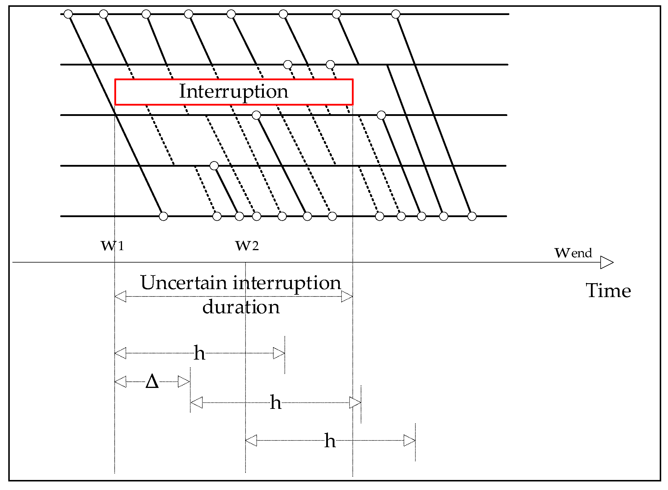
4.1. Rolling Horizon Algorithm

The rolling horizon algorithm is a dynamic optimization approach that sequentially addresses problems by repeatedly solving a finite-time horizon optimization problem over a moving window of time. This method is particularly useful for systems where the operational conditions are subject to continuous change, and it allows for the incorporation of the most recent information into the decision-making process. The algorithm involves setting a finite time horizon, solving an optimization problem within this horizon, implementing the first part of the solution, and then rolling the horizon to the next period to solve a new optimization problem with updated information. This iterative process enables the algorithm to adapt to changes in system dynamics and constraints over time. The rolling horizon algorithm has been widely applied in various fields, including transportation [38], energy [39], and control [40], due to its ability to handle complex, dynamic systems effectively.

In this section, we use the rolling horizon algorithm to deal with the uncertain duration of the interruption. The main process is as follows:

The schematic diagram of the rolling horizon algorithm is shown in Figure 2. Its main purpose is to solve the problem of the uncertain duration of the interruption. The algorithm can solve the train timetable in stages. In the figure, $w_1$ and $w_2$ represent the start time of each stage, $h$ is the time domain length of each stage, and $\Delta$ is the rolling step size of the algorithm. $w_1$ represents the start time of the interruption, $w_2$ represents the time when the information of the interruption updates, and $w_{\mathrm{end}}$ represents the end time of the algorithm. The rolling horizon algorithm starts solving the train timetable from time $w_1$, only solves the train timetable for the $w_1~w_1+h$ period in each stage, and issues the timetable for the $w_1~w_1+\Delta$ period to the train dispatcher to instruct train operation. The next stage starts from $w_1+\Delta$ and repeats this process. When the interruption duration information is updated (time $w_2$), it outputs the train timetable before time $w_2$ and starts a new solving phase with $w_2$ as the starting time. It scrolls in this way until the whole train timetable for the entire period is solved.

In the initial stage, the algorithm is first inputted with information such as the planned train timetable, the duration of the interruption, and the rolling step size of the rolling horizon optimization algorithm. Before the interruption occurs, all trains run according to the original planned train timetable. After the interruption occurs, three parameters should be inputted at each stage: ① to confirm the range of the train timetable that needs to be adjusted, the length of the solution period needs to be input; ② to ensure that the subsequent train operation adjustment plan is based on the previous stage, it is necessary to input the adjusted train timetable before this stage; ③ it is necessary to input the duration of the interruption determined by the operation department and the dispatcher at the beginning of this stage. Then, a train operation adjustment model considering the interruption (mentioned in Section 3) is adopted to solve the train operation plan during this period, and the adjusted train timetable is obtained. If the train operation adjustment for the entire period has not been completed and there are trains that have not been rescheduled, the next stage of solving will be entered. During this period, the duration of the interruption will be continuously updated based on the information of interruption duration until all trains have been rescheduled.

4.2. The Introduction of the NSGA-II Algorithm

In handling multi-objective problems, the MOEA/D method has been widely recognized [41,42] for its effectiveness. At the same time, NSGA-II (non-dominated sorting genetic algorithm II) is also a widely used multi-objective optimization algorithm introduced by Deb et al. [43] in 2002. It is an evolutionary algorithm designed for solving multi-objective optimization problems. It aims to generate a set of Pareto-optimal solutions by balancing convergence to the Pareto front and maintaining diversity among the solutions. Unlike single-objective optimization, NSGA-II optimizes multiple conflicting objectives simultaneously, producing a set of trade-off solutions rather than a single optimal solution.

The NSGA-II algorithm has been applied in a variety of fields like energy [44], finance [45], complex systems [46], and transportation [47]. It improves upon its predecessor, NSGA, by addressing computational complexity and elitism, as well as introducing a novel crowding distance mechanism for better diversity maintenance.

4.3. Deep Learning Model Data Preparation and Training

The NSGA-II algorithm has demonstrated significant advantages in solving complex optimization problems due to its excellent global search capability and parallel processing characteristics. However, the insufficient local search capability of this algorithm often leads to low search efficiency, and it may not frequently explore new solution regions, which can result in a decrease in population diversity. This reduction in population diversity makes the algorithm more prone to falling into local optima, causing premature convergence of the algorithm. This limitation restricts its application effectiveness in dealing with complex optimization problems to some extent.

To overcome these shortcomings, we have designed a deep-learning-embedded NSGA-II algorithm that can effectively compensate for the shortcomings of the traditional NSGA-II algorithm. When facing complex optimization problems, this algorithm replaces the random selection of crossover and mutation sites with the prediction of a trained deep learning model. By deeply learning the inherent rules of the data and utilizing its pattern recognition ability, it greatly reduces invalid searches, improves the efficiency of local searches, and enables the algorithm to fully explore different regions in the solution space. This helps to improve the diversity of the population and avoid premature convergence of the algorithm, thus effectively approaching the global optimal solution in the later stages of iteration.

Among common deep learning models, MLP has advantages in regression analysis and various data prediction. Therefore, we choose the MLP model to learn and predict crossover and mutation gene loci. Based on the characteristics of the model, the following training steps are designed:

4.3.1. Obtain Training Data for Deep Learning Models

In order to enhance the generalization ability and effectiveness of the model, this paper is based on the actual train schedules of the Beijing–Guangzhou high-speed railway, the Tianjin–Qinhuangdao high-speed railway, and the Jinan–Qingdao high-speed railway. We used the NSGA-II algorithm designed in this paper for iterative calculations, and all the data obtained from the iterations were used as training data for the deep learning model. The following is an introduction to the data acquisition process using the Beijing–Guangzhou high-speed railway as an example.

Step 1: Initialize the population. The number of individuals in the population is set to N, and each individual consists of three gene fragments. The meanings of each gene fragment are described in Section 4.4.1. According to the train timetable of the Beijing–Guangzhou high-speed railway from 6:00 to 24:00, the parameters of the model are set, and the initial values of each gene fragment of the individuals in the population are determined.

Step 2: Calculate the fitness value of each individual based on the fitness function (described in Section 4.4.4) and simultaneously calculate the characteristic values of each gene site (the column) in each gene fragment of each individual.

Step 3: Select the better individuals from the parent and offspring generations (starting from the second generation) based on their fitness values to enter the next generation and form a new population.

Step 4: Randomly select positions for crossover and mutation, with a crossover rate of 35% and a mutation rate of 8%.

Step 5: Determine whether the algorithm has iterated to 400 generations. If it has reached 400 generations, proceed to Step 6; otherwise, jump back to Step 2.

Step 6: Output the best individual in the current population.

4.3.2. Train the Deep Learning Models

The first step is to standardize the fitness values and feature values of each gene fragment obtained in Section 4.4.1 to make them suitable for the input of the neural network. There are 400 generations of data; of these, 200 generations are randomly selected as the training set, and the remaining 200 generations as the test set. The second step is to build an MLP model for each gene fragment. Taking gene fragment 2 as an example, suppose it has $n$ columns, representing $n$ trains. Each column is regarded as a gene locus, with a total of $n$ gene loci. Each gene locus corresponds to a feature value. In the input layer of the MLP model, each neuron receives the feature value of one gene locus, so the input layer is set to $n$ neurons. Three hidden layers are chosen, with the first hidden layer set to $\left(2/3\right)n$ neurons, the second hidden layer set to ${\left(2/3\right)}^{2}n$ neurons, and the third hidden layer set to ${\left(2/3\right)}^{3}n$ neurons. The output layer is set to 1 neuron to predict the fitness value. The activation function of the hidden layers is ReLU, and the activation function of the output layer is a linear activation function. The He initialization method is used for the initialization of the weights. The third step is to train the model. According to the data volume of this example, the number of epochs is set to 200. At the same time, early stopping is used to monitor the model to prevent overfitting. In each epoch, the predicted output of the model is compared with the actual fitness value, and the loss function is set as mean squared error (MSE). Then, the gradient is calculated using backpropagation, and finally, the weights of the model are updated using the gradient calculated by Adam, which is used in the PyTorch 2.0 framework. The trained model is eventually obtained.

4.4. The Process of the NSGA-II Algorithm Embedded in Deep Learning

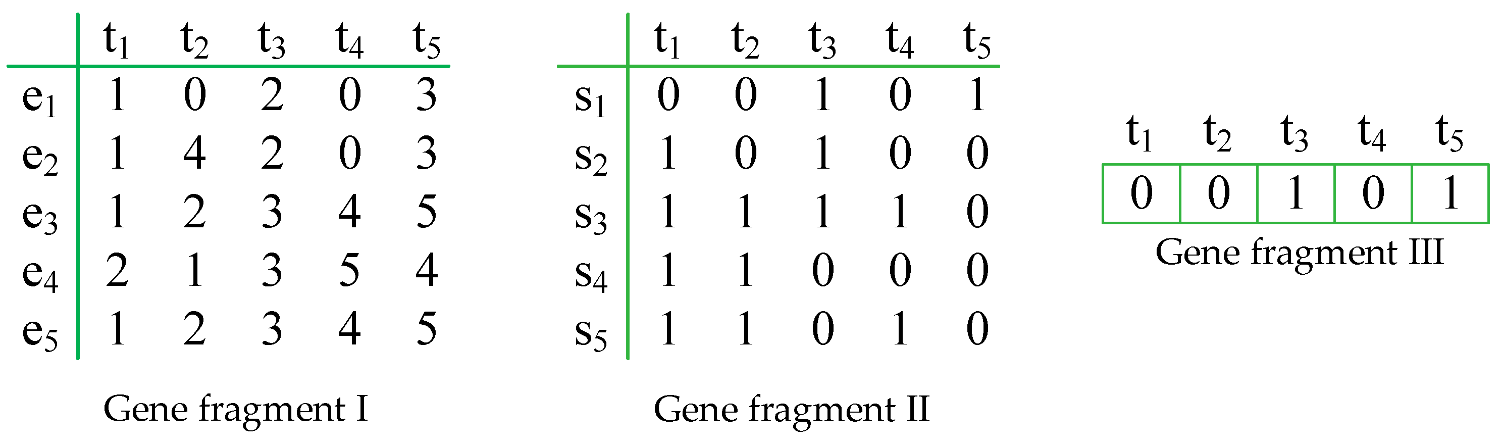
4.4.1. Gene Fragments

In this approach, solutions are represented indirectly through parameters, which are subsequently utilized in a unique decoding process to derive the solution. As depicted in Figure 3, each chromosome consists of three segments of genes.

Gene fragment I denotes the sequence of trains across various sections. This segment is structured as a two-dimensional matrix, where the horizontal axis corresponds to trains and the vertical axis represents sections. For example, in section $e_2$, train $t_1$ is the first train to pass through, $t_3$ is the second train, $t_5$ is the third, and $t_2$ is the fourth, while $t_4$ does not pass through section $e_2$. Gene segment II represents the train’s stop situation at each station, which is a matrix. The horizontal axis represents the stations, and the vertical axis represents the train. The values in the matrix are binary variables, with a value of 1 representing that the train stops at the station and 0 representing that it does not stop. The third gene fragment represents the cancelation scheme of the trains. A value of 1 represents the train being cancelled, while a value of 0 represents it not being cancelled.

4.4.2. Initialize the Population

Initialize the population based on the existing train timetable. Gene fragment I is built upon the original train timetable, while gene fragments II and III are generated randomly and may not adhere to the necessary constraints. As a result, it is crucial to assess all initial solutions to determine a set of feasible solutions. To make the infeasible solutions feasible, the following adjustments will be made, as shown in Algorithms 1 and 2:

• The cancelled trains will not serve any passengers. The sequence values in its gene segment I and the station-stop values in its gene segment II will be 0 in all sections.

Algorithm 1. Handle the cancelled trains.

Step 1. Determine the value of each variable ${\psi }_t^e$ based on gene fragment I. Determine the value of each variable ${\epsilon }_j^t$ based on gene fragment II. Determine the value of each variable ${\delta }^t$ based on gene fragment III.         Step 2. Create set $T$ and add all the train $t$ to $T$. Create set $E$ and add all the section $e$ to $E$. Create set $J$ and add all the station $j$ to $J$,

Step 3. Determine the values of variables ${\psi }_t^e$ and ${\epsilon }_j^t$ of the cancelled trains.         For each train $t\in T$:             If ${\delta }^t=1$               For each section $e\in E$:                  If ${\psi }_t^e\ne 0$                     Let ${\psi }_t^e=0$                  If ${\psi }_t^e=0$                     Continue               For each station $j\in J$:                  If ${\epsilon }_j^t\ne 0$                     Let ${\epsilon }_j^t=0$                  If ${\epsilon }_j^t=0$                     Continue           If ${\delta }^t=0$               Continue

2.

After the initialization of the solutions, there may be some infeasible sequence of the trains, such as 6,1,3,0,4,5,7, which should be adjusted to 5,1,2,0,3,4,6.

Algorithm 2. Find the infeasible sequence and adjust gene fragment I.

Step 1. Obtain the value of each variable ${\psi }_t^e$ from the result of Algorithm 1.         Step 2. Create set $T$ and add all the train $t$ to $T$. Create set $E$ and add all the section $e$ to $E$.         Step 3. Get the feasible sequence of the trains in each section.         Create set $TEM$.         For each section $e\in E$:            For each train $t\in T$:               Add ${\psi }_t^e$ to set $TEM$.            Check whether all the nonzero ${\psi }_t^e$ in $TEM$ is continuous, and begin with value 1.            If not,               Adjust all nonzero ${\psi }_t^e$ in $TEM$ to consecutive integers in their original order

If yes,               Clear set $TEM$.               Continue.

4.4.3. Chromosome Decoding

Chromosomes in this study are composed of three distinct genetic segments, each representing a critical aspect of railway operations: the sequencing scheme for train departures, the stopping scheme for the train at the station, and the cancellation scheme for train services. The decoding of these genetic segments is essential to extract the train timetable and passenger flow allocation plan. Consequently, the decoding process is meticulously divided into two principal stages to ensure accurate interpretation and application of the genetic information encoded within the chromosomes.

• Obtain train timetable

Step 1: Determine the cancellation of the train through gene fragment III and adjust the values of gene fragments I and II of the cancelled trains. Change all the column values in the gene fragment matrix of the cancelled train to 0. This step can determine the value of the variable ${\delta }^t$.

Step 2: Based on the gene fragments I, II, and III at this time, we can obtain the order of all trains in each section and whether the trains stop at the stations, and determine the values of variables ${\epsilon }_j^t$, ${\psi }_t^e$, and ${\eta }_{j,j+1}^{t,t\text{'}}$.

Step 3: Under the condition of known train sequence in the sections and the stopping plan, and considering the basic constraints of the train timetable, including the constraints of the time range, the constraints of station tracking interval, the constraints of station stop time, and the constraints of train operation time, we can calculate and obtain the actual arrival time ${\tau }_j^t$ and actual departure time ${\theta }_j^t$. It is worth mentioning that in this step, we applied the rolling horizon algorithm mentioned in Section 4.1 to process the uncertain duration of the interruption. At this point, the new train timetable has been formed.

2.

Distribution of affected passenger flow

The passenger flow that has not been affected by the interruption is served by the original train, and only the passenger flow affected by the interruption is allocated. Algorithm 3 presents the allocation process for affected passenger flow:

Algorithm 3. Allocate affected passenger flow

Step 1. Create affected passenger set $AP$ and add all affected passenger demands $x$ to it. Create affected trains set $AT$ and add all affected trains $t$ to it.         Step 2. Allocate passenger flow to trains.         For each passenger demand $x\in AP$:            For each train $t\in AT$:               Judge whether the total number of passengers does not exceed train $t$’s seating capacity after adding passenger demand $x$.               If yes,                  Judge whether the departure time of the passenger demand $x$ is later than the departure time of train $t$ at the origin station of the passenger demand $x$.                     If yes,                        Judge whether train $t$ stops at the departure and arrival stations of passenger demand $x$.                        If yes,                           Let train $t$ serve passenger demand $x$ and remove passenger demand from set $AP$.                        If not,                           Continue;                     If not,                        Continue;                  If not,                     Continue;

Step 3. Cancel the remaining passenger demands in set $AP$.

At this point, the values of variables ${\mu }_{t\text{'}}^{t,x}$, ${\delta }^{t,x}$, and ${\sigma }_{t\text{'}}^{t,x}$ have been determined.

4.4.4. Fitness Calculation

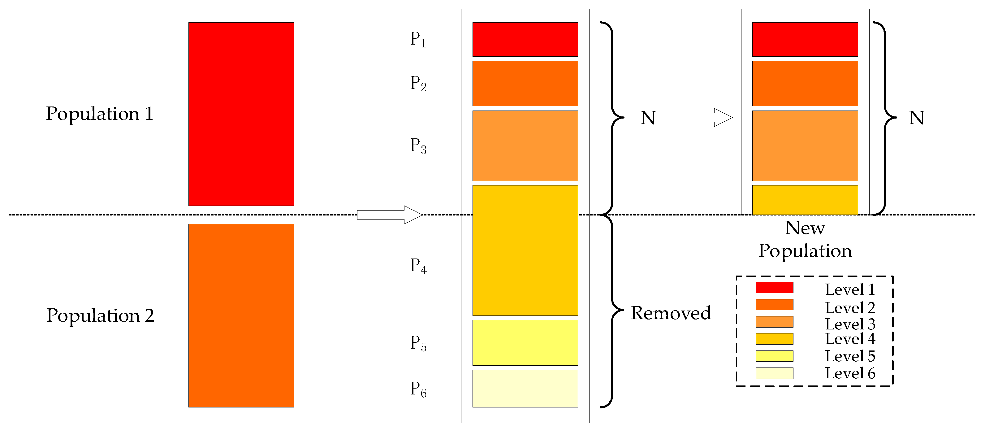
The two fitness functions are as follows:

$$f_1=\min c_1{\displaystyle \sum _{t\in T}{\displaystyle \sum _{x\in X}({\delta }^{t,x}\times T_{\mathrm{can}}^{\mathrm{pas}}\times N_{\mathrm{pas}}^{t,x})}}+c_2{\displaystyle \sum _{t\in T}({\tau }_{S_{\mathrm{end}}^t}^t-T_{\mathrm{pa}}^{t,S_{\mathrm{end}}^t})\times (N_{\mathrm{pp}}^t+{\displaystyle \sum _{t\text{'}\in T_{\mathrm{aff}}}{\displaystyle \sum _{x\in X}{\sigma }_t^{t\text{'},x}}})}$$

(21)

$$f_2=\min {\displaystyle \sum _{t\in T}{\displaystyle \sum _{j=S_{\mathrm{start}}^t}^{S_{\mathrm{end}}^t}{D}_{\mathrm{btw}}^{j,j+1}\times C_{\mathrm{oper}}^{\mathrm{train}}\times {\delta }^t}}+{\displaystyle \sum _{t\in T}{\displaystyle \sum _{x\in X}{\displaystyle \sum _{j=S_{start}^{t,x}}^{S_{end}^{t,x}}{N}_{\mathrm{pas}}^{t,x}\times C_{\mathrm{oper}}^{\mathrm{pas}}\times D_{\mathrm{btw}}^{j,j+1}\times {\delta }^{t,x}}}}$$

(22)

Function $f_1$ is the decline in passenger service quality, and function $f_2$ is total operating cost. After obtaining the two functions, the Pareto front is generated with the use of the method mentioned in 4.2.3 in every iteration.

4.4.5. Selection

To identify and retain individuals of higher quality from the existing population for the purpose of generating a new population, a selection process must be implemented.

After the calculation in 4.4.4, we obtained a group of Pareto fronts for the current population. Firstly, we select the Pareto front $P_1$ at the first level, as it is currently the best solution, so we need to focus on selecting it. If the length of $P_1$ is less than the individual number ($N$) of the new population, then choose $P_1$ to add to the new population, and perform the same operation on $P_2$, $P_3$ …, until the remaining number of individuals in the new population is insufficient to accommodate a complete Pareto front. Then, assuming that $P_i$ is the last Pareto front that cannot be accommodated, arrange the individuals in $P_i$ in descending order by crowding distance, and select the individuals ranked higher and add them to the new population until the size of the new population reaches $N$. A diagram of the selection process is shown in Figure 4. In this figure, different colored blocks represent solution sets with different dominance levels (Level 1 is the highest dominance level). The lighter the color, the lower the dominance level of the solutions in the set, meaning that they are dominated by more other solutions.

4.4.6. Crossover and Mutation

• Crossover

In the process of the genetic algorithm, one of the operators is crossover. Two chromosomes will be selected to create a new chromosome. The selection of each chromosome is based on a probability $P_{chrom}$, which is influenced by its non-dominated sorting rank. Specifically, chromosomes with higher non-dominated sorting ranks are more likely to be chosen for crossover. This approach ensures that chromosomes with better fitness have a higher chance of contributing to the next generation.

For gene fragment II and gene fragment III, we use the deep learning model (MLP) trained in Section 4.3 to calculate and select the gene locus corresponding to the neuron with the highest weight as the crossover locus, replacing the method of randomly selecting crossover loci, as in traditional genetic algorithms. For gene fragment I, we choose one train sequence set from the two parent chromosomes to serve as gene fragment I in the newly formed chromosome.

2.

Mutation

Another operator is mutation. The mutation rate is set to 16%. The mutation operations are performed on three gene fragments, respectively.

For gene fragment II and gene fragment III, each chromosome has a 16% chance of being selected, and the trained deep learning model mentioned in Section 4.3 is used to choose the mutation locus. Given that the variables in gene fragments II and III are binary variables, the mutation operation results in a change of the selected gene’s value, either from 0 to 1 or from 1 to 0.

For gene fragment I, each chromosome has a 16% chance of being selected, and the mutation locus is chosen by the trained deep learning model mentioned in Section 4.3. However, gene fragment I is the train sequence matrix, whose values are not binary variables. Therefore, after we obtain the mutation locus, we choose the train corresponding to the mutation locus and let this train overtake the adjacent train that is in front of it at a certain station.

After crossover and mutation, a series of new individuals are generated, and a new generation of the population is formed with these new individuals.

4.4.7. Update Weights of MLP Model

First, calculate the loss function (MSE) based on the predicted output of the comparison model and the true fitness value of the contemporary population. Then, use backpropagation to calculate the gradient. Finally, update the weights of the model using the gradient calculated by Adam.

4.4.8. Check Termination Conditions

The algorithm terminates and outputs the final results under two conditions: firstly, if no new individuals are added to the Pareto front for 30 consecutive iterations, indicating that the population has stabilized and further improvements are unlikely; secondly, if the total number of iterations reaches a pre-set threshold.

4.5. The Process of the Hybrid Algorithm

Step 1: Input information such as the planned train timetable, the duration of the interruption determined by the operation department and the dispatcher, and the rolling step size of the rolling horizon optimization algorithm.

Step 2: Use the NSGA-II algorithm embedded in deep learning to solve the train timetable.

Step 3: Randomly select a solution from the Pareto front obtained in Step 2 and determine whether the train timetable has been completed for the entire period, that is, whether there are trains that have not been rescheduled. If there are trains that have not been rescheduled, return to Step 1, renew the train timetable based on Step 2, and renew the latest duration of the interruption judged by the operation department and the dispatcher. If there are no trains that have not been rescheduled, turn to Step 4.

Step 4: Output the final solution.

The whole process of the hybrid algorithm is shown as Figure 5:

5. Case Study

In this chapter, we conduct a series of experiments to evaluate our model and algorithm. All computational experiments were executed on a system equipped with an Intel (R) Xeon (R) processor featuring 32 cores and 64GB of RAM.

5.1. Basic Data

Taking the train schedule of a certain day from 6:00 to 24:00 on the Beijing–Shanghai high-speed railway as an example, we validate the model and algorithm proposed in this paper. The Beijing–Shanghai high-speed railway starts at Beijing South Station and ends at Shanghai Hongqiao Station, with a total length of 1318 km. As Figure 6 shows, it has a total of 23 stations and 22 sections, and each station corresponds to a numerical number. The daily train operation count is 550, and it is assumed that all trains operate at a speed of 300 km/h.

The parameters of the model are detailed in

Table 4. Value of the parameters.

Parameter	Value
$T_{\mathrm{exs}}^j$ The extra starting time	2 min
$T_{\mathrm{exd}}^j$ The extra stopping time	3 min
$T_{\mathrm{stop}}^j$ Train stopping time at the station	3 min
$C_{\mathrm{oper}}^{\mathrm{train}}$ The cost per kilometer for each train	330 yuan
$C_{\mathrm{oper}}^{\mathrm{pas}}$ The cost per kilometer for each passenger	0.114 yuan
$N_{\mathrm{cap}}^t$ The passenger carrying capacity	1200 people
$T_{\mathrm{can}}^{\mathrm{pas}}$ Penalty time for the passenger flow cancellation	720 min
$T_{btt}$ Train tracking intervals	4 min
$T_{\mathrm{amd}}$ The maximum allowable additional dwell time	20 min

.

The distance and operating time of each section of the Beijing—Shanghai high-speed railway are shown in

Table 5. The distance and operating time of sections.

Section	Distance (km)	Time (min)	Section	Distance (km)	Time (min)
1–2	59.5	18	12–13	88.0	20
2–3	62.6	14	13–14	54.3	12
3–4	87.9	20	14–15	62.0	14
4–5	103.8	23	15–16	59.0	14
5–6	92.2	21	16–17	65.4	15
6–7	58.7	14	17–18	28.6	7
7–8	70.4	15	18–19	32.4	8
8–9	56	12	19–20	57.4	13
9–10	36.1	8	20–21	26.8	6
10–11	64.4	14	21–22	31.4	7
11–12	67.2	15	22–23	44	13

.

5.2. Effectiveness Analysis of the Model and Algorithm

5.2.1. The Comparison Before and After Iteration

We set up a one-direction interruption in section 6–7 starting at 11:00 and used the proposed hybrid algorithm to solve the train timetable. The rolling step size was set to 30 min. For the NSGA-II, the population size was 30, and the maximum number of iterations was set to 200 generations. Based on the above conditions, we have set up three types of experiments in terms of interruption duration: small-scale, medium-scale, and large-scale. In the small-scale experiment, it is assumed that during the iteration process, the first four predicted interruption durations are 95, 80, 68, and 65 (minutes), respectively. The predicted interruption durations are 165, 154, 142, 130, 128, and 123 for the medium-scale and 301, 318, 279, 252, 249, 243, 239, 226, and 225 for the large-scale experiments, respectively. For the small-scale and medium-scale experiment, the solving period is 6 h, and for the large-scale experiment, the solving period is 12 h.

For the objective value comparison before and after iteration, we take the small-scale experiment as an example and have drawn a comparison chart showing before and after iteration, which is shown in Figure 7.

Figure 7a shows the solutions before iteration, and Figure 7b shows the solutions after iteration. The horizontal axis represents the objective decline in passenger service quality, and the vertical axis represents the objective total operating cost. The specific numerical analysis of the small-scale experiment (65 min), medium-scale experiment (123 min), and large-scale experiment (225 min) is shown in

Table 6. Comparison before and after iteration of three experiments.

		Average Decline in Passenger Service Quality	Average Total Operating Cost
Small-scale experiment (65 min)	Before iteration	6,991,740.03	26,270,525.87
	After iteration	5,854,112.53	22,178,020.07
	Optimization rate	16.27%	15.58%
Medium-scale experiment (123 min)	Before iteration	11,787,649.67	30,745,108.43
	After iteration	9,913,618.23	26,389,165.17
	Optimization rate	15.90%	14.17%
Large-scale experiment (225 min)	Before iteration	15,193,746.93	43,718,573.23
	After iteration	13,222,301.74	37,931,957.07
	Optimization rate	12.98%	13.23%

.

As Table 6 shows, the optimization results demonstrate a significant improvement in both objective functions. Overall, the objective function representing the decline in passenger service quality decreased by 16.27%, 15.90%, and 12.98% in the small-scale, medium-scale, and large-scale experiments, respectively. Meanwhile, the total operating costs decreased by 15.58%, 14.17%, and 13.23% in the three types of experiments, respectively. These improvements indicate that the hybrid algorithm effectively enhances the solution quality, making significant achievements in terms of reducing the decline in passenger service quality and lowering operating costs. It is worth noting that, as shown in the table, with the increasing scale of experiments, there is a slight decrease in the optimization rate of the objective function, indicating that the expansion of the experimental scale has some impact on the solution quality. However, the impact is not significant and remains within an acceptable range.

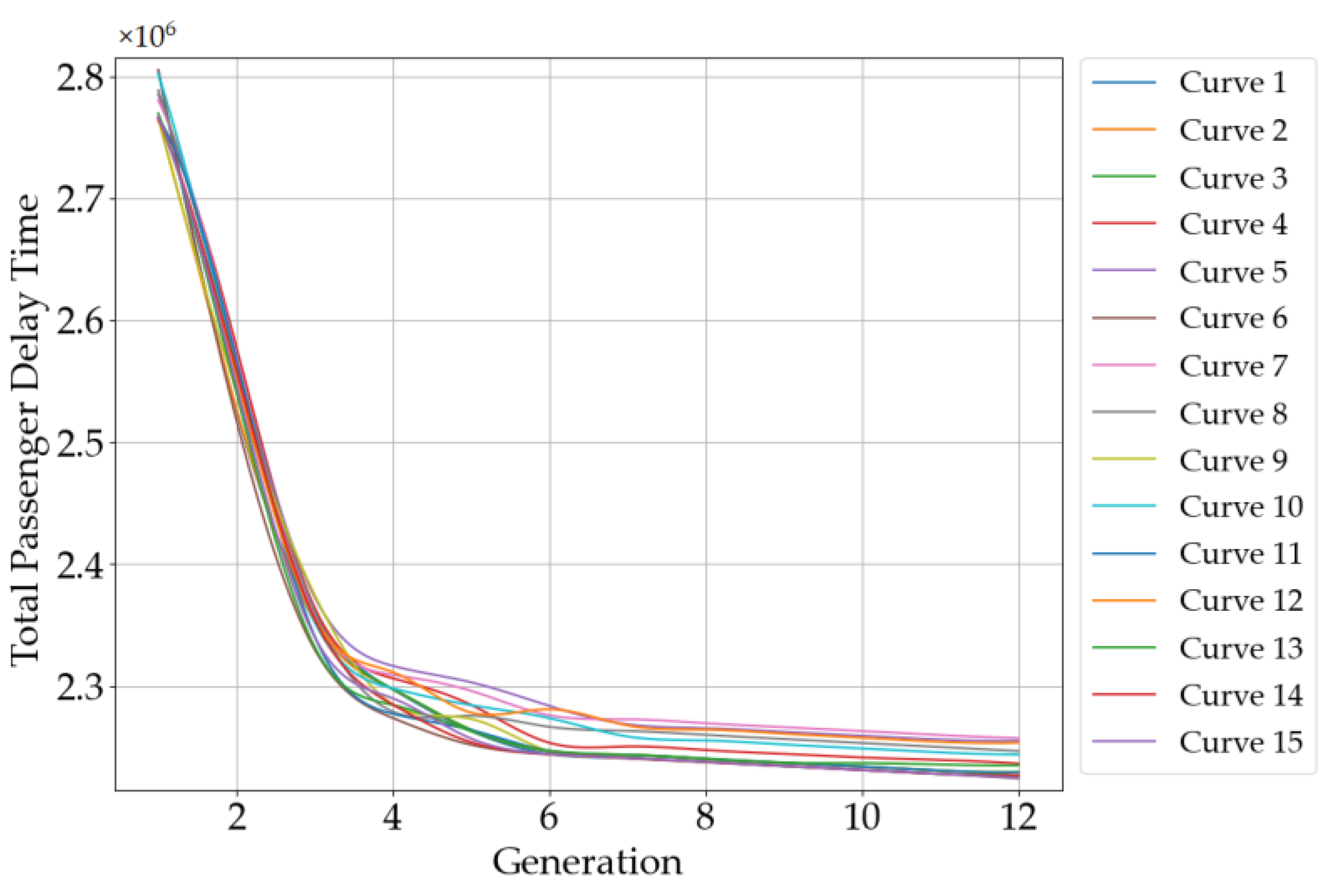
5.2.2. The Converging Trend of the Objectives

We selected the medium-scale experiment and plotted the iteration curves of the algorithm rolling through 12 iterations for the two objective functions, as shown in Figure 8.

Because the rolling window of each iteration is half an hour, the time from the start of the interruption to the end of the iteration varies for each iteration. For comparison purposes, we divided the result of each iteration by the total duration of that iteration to obtain the objective function value per unit time (per hour) and plotted the curve.

Throughout the optimization process, the objective function value showed a gradually decreasing trend, indicating that the optimization algorithm can effectively reduce the decline in passenger service quality and total operating cost. This indicates that the optimization method used can quickly solve delay problems, adjusting the system in the early stages and gradually stabilizing in the later stages, with relatively less room for further optimization. Additionally, in both small-scale and large-scale experiments, the trend of the convergence curves was generally consistent with that of the medium-scale experiments, exhibiting a trend of rapid decline in the initial stages and a slower decline in the later stages.

Specifically, the first half of the curve decreases rapidly, reflecting the significant adjustment effect of the problem in the initial stage. The gentle decline in the latter half of the curve indicates that the optimization process has gradually approached a stable solution. This is a typical characteristic of optimization algorithm convergence, indicating that the problem is approaching the optimal solution.

5.2.3. Stability Analysis of the Algorithms

To analyze the stability of the algorithm, we conducted 15 repeated large-scale experiments based on the experimental parameters in Section 5.2.1. The experimental results are shown in

Table 7. The results of 15 repeated experiments.

	Average Decline in Passenger Service Quality	Average Total Operating Cost	Time
1	17,981,400.10	37,675,865.81	2628
2	17,663,376.74	38,050,094.80	2636
3	18,428,048.81	36,580,427.13	2619
4	17,703,014.19	38,463,797.62	2676
5	17,179,913.87	38,607,104.42	2634
6	18,697,415.43	36,444,626.11	2632
7	17,499,388.73	39,016,232.10	2605
8	17,729,263.70	38,077,359.00	2598
9	17,962,408.54	37,110,804.84	2670
10	17,840,205.92	36,307,839.33	2642
11	18,480,678.37	37,285,517.82	2621
12	17,546,266.63	38,494,872.35	2615
13	17,155,270.56	38,054,814.79	2662
14	17,330,109.37	37,879,640.83	2635
15	17,134,583.91	38,944,548.68	2683
Mean value	17,755,422.99	37,799,569.71	2637.07
Std	472,285.04	851,699.54	24.64
Proportion of std	2.66%	2.25%	0.93%

.

We can see from Table 7 that the maximum objective 1 of 15 repeated experiments is 18,697,415.43, from experiment 6; the minimum objective 1 is 17,134,583.91, from experiment 15. The coefficient of variation is a relative indicator used to measure the degree of dispersion of data. It is the ratio of the difference between the maximum and minimum values in a set of data to the average value. The smaller the coefficient of variation, the lower the degree of dispersion of the data and the better the stability of the data. Usually, if the coefficient of variation is less than 0.1, it is considered that the stability of the data in this group is good. The coefficient of variation of objective 1 is (18,697,415.43–17,134,583.91)/17,755,422.99 = 0.088, which is less than 0.1, indicating that our algorithm has considerable reliability and reproducibility. In addition, the proportion of std is 2.66% and 2.25%, respectively, which also can prove this point.

As shown in Figure 9, we have plotted the convergence curves of objective 1 over 15 experiments. Different from small-scale and medium-scale experiment, the large-scale experiment has a duration of 12 h and a total of 24 iterations. All convergence curves decrease and converge to a certain value. The trends and convergence values between each curve are not significantly different, indicating that our algorithm has good stability. In addition, in the convergence curves of the two objective functions, we find that in the first eight generations, the rate of decline of the objective function value is the fastest, much faster than that of the other generations. This is because, in this experiment, the predicted interruption duration of the first eight generations is continuously shortening, resulting in a faster rate of decline in passenger cancellation and passenger delay; therefore, the value of objective 1 declines fast. Starting from the ninth prediction of interruption duration, the interruption has already ended, and the interruption duration has been determined, so the rate of decrease in the objective function value slows down.

5.3. Comparative Analysis of Hybrid Algorithm and Single Algorithm

In this section, we set up a one-direction interruption in section 14–15 starting at 9:00 and used different algorithms to solve the train timetable over a 6 h and a 12 h period: (1) only the rolling horizon algorithm (RHA); (2) only the NSGA-II algorithm (NSGA-II); (3) the genetic algorithm with embedded deep learning (NSGA-II + DL); (4) hybrid algorithm using both rolling horizon algorithm and genetic algorithm embedded in deep learning (RHA + NSGA-II + DL). To make the results comparable, we set the same interruption duration in experiments 1–4 (6 h) and 5–8 (12 h), respectively. For experiments 2, 3, 6, and 7, the population size was 30, and the maximum number of iterations was set to 200 generations. For experiments 1, 4, 5, and 8, the rolling step size is set to 30 min, and the predicted duration is as follows. The experiment results are shown in

Table 8. Comparison of solution quality and effectiveness of examples.

Experiment	Algorithm	Interruption Duration/Predicted Duration (min)	Objective 1	Objective 2	Convergent Generation	Calculation Time (s)
1	NSGA-II	60	6,735,122	24,624,726	130	2301
2	RHA + NSGA-II	82, 75, 66, 60	6,473,291	23,894,763	-	2015
3	NSGA-II + DL	60	5,983,373	23,595,738	91	2268
4	RHA + NSGA-II + DL	82, 75, 66, 60	5,729,385	22,985,716	-	1698
5	NSGA-II	120	12,350,174	46,592,385	139	4583
6	RHA + NSGA-II	152, 146, 138, 132, 124, 118, 120	11,641,787	43,206,595	-	3673
7	NSGA-II + DL	120	11,556,720	39,902,857	112	4489
8	RHA + NSGA-II + DL	152, 146, 138, 132, 124, 118, 120	10,427,757	39,038,572	-	2689

. We will analyze this from two aspects: (1) optimization performance and convergence and (2) computational efficiency.

5.3.1. Optimization Performance

(1)

Objective 1: average decline in passengers service quality

Among the compared algorithms, the hybrid algorithm RHA + NSGA-II + DL exhibits the best optimization performance in both the 60 min scenario (with a value of 5,729,385) and the 120 min scenario (with a value of 10,427,757). Notably, NSGA-II + DL (experiment 3) also shows significant improvement, achieving a value of 5,983,373, compared to NSGA-II (experiment 1), which has a value of 6,735,122. The integration of deep learning notably enhances the optimization outcomes.

While RHA + NSGA-II (experiment 2) outperforms NSGA-II, with a value of 6,473,291 (an improvement over NSGA-II’s 6735122), it still lags behind NSGA-II + DL (5983373) and RHA + NSGA-II + DL (5729385). This suggests that although RHA + NSGA-II combines the strengths of the rolling horizon algorithm, it does not significantly improve the objective value as effectively as deep-learning-based algorithms.

(2)

Objective 2: average total operating cost

Similarly, the hybrid algorithm RHA + NSGA-II + DL performs the best in objective 2, with values of 22,985,716 (for 60 min) and 39,038,572 (for 120 min), clearly outperforming NSGA-II (values: 24,624,726 and 46,592,385) and NSGA-II + DL (values: 23,595,738 and 39,902,857). RHA + NSGA-II (experiment 2) shows an improvement over NSGA-II with a value of 23,894,763, but it still lags behind the deep-learning-based algorithms.

5.3.2. Convergence and Computational Efficiency

(1)

Convergence generation

Hybrid algorithms RHA + NSGA-II + DL and NSGA-II + DL show faster convergence. NSGA-II + DL converges in 91 generations for 60 min and 112 generations for 120 min, while NSGA-II requires 130 generations for 60 min and 139 generations for 120 min, indicating that after combining deep learning, the solution results of the algorithm can converge more quickly. Since the role of RHA in solving the timetable is to divide the solving process into small segments, and it does not have convergence itself, the convergence generation of experiments 2, 4, 6, and 8 will not be discussed here.

(2)

Calculation time

RHA + NSGA-II + DL demonstrates the best computational efficiency, with calculation times of 1698 s for 60 min and 2689 s for 120 min. Compared to other single algorithms or algorithm combinations when the interruption duration is eventually 60 min, RHA + NSGA-II + DL has improved the computational efficiency by 26.21%, 15.73%, and 25.13%, respectively.

RHA + NSGA-II has a calculation time of 2015 s, better than NSGA-II, but still longer than RHA + NSGA-II + DL. At the same time, we also noticed that the computational efficiency of RHA + NSGA-II + DL is better than that of NSGA-II + DL, and the computational efficiency of RHA + NSGA-II is better than that of NSGA-II, indicating that the addition of RHA can effectively reduce solving time and improve solving efficiency. The reason is that RHA divides the entire lengthy solving process into small segments, reducing the scale and difficulty of the solution and improving the efficiency of the solution.

The hybrid algorithm RHA + NSGA-II + DL performs best in both optimization quality and computational efficiency, providing the optimal solution, especially for handling varying interruption durations. The incorporation of deep learning significantly improves convergence speed and optimization results while reducing calculation time. Although RHA + NSGA-II integrates the advantages of the rolling horizon algorithm and NSGA-II, its performance still lags behind NSGA-II + DL and RHA + NSGA-II + DL, particularly in terms of objective values and computational efficiency.

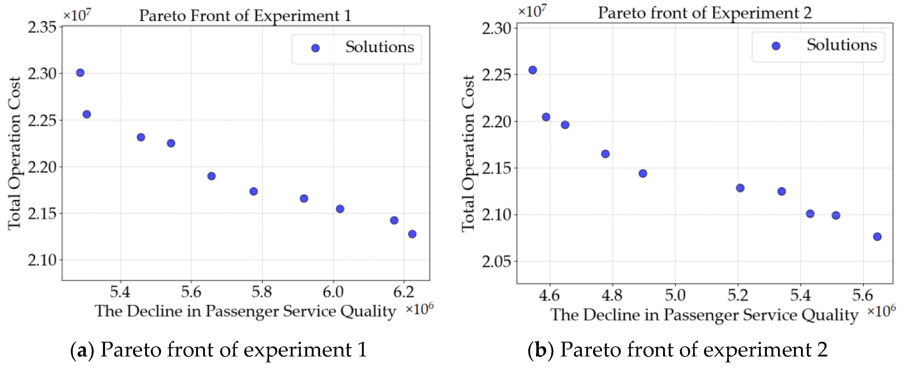
5.4. Pareto Front Analysis

We set up two experiments with a one-direction interruption in sections 11–12 and 18–19 starting at 15:00 and used the proposed hybrid algorithm to solve the train timetable over a 6 h period. The rolling step size was set to 30 min. It was assumed that during the iteration process, the first four predicted interruption durations were 87, 76, 73, and 66 (min), respectively. For the NSGA-II, the population size was 30, and the maximum number of iterations was set to 200 generations.

We selected the last generation, which consists of 30 individuals, for the analysis and drew scatter plots of the Pareto front, which includes 10 individuals and 10 individuals, respectively, as Figure 10 shows.

5.4.1. Analysis of a Single Pareto Front Scatter Plot

The Pareto front shows the relationship between passenger service quality and operational cost, providing a clear indication of the trade-off between these two conflicting objectives. As expected, a higher service quality typically corresponds to a higher operational cost. This relationship is observed in the Pareto front, where the solutions with better service quality tend to have higher values for objective 2 (total operating cost). For the same reasons, lower operating costs tend to come at the expense of lower passenger service quality. The solutions in the Pareto front represent different trade-offs, where improving one objective often leads to reducing the other.

For each front, these solutions exhibit diversity in terms of passenger service quality and operational costs, offering decision makers a range of different schemes to choose from depending on their priorities. For instance, if the priority is to minimize operational costs, the algorithm provides solutions with lower costs but with some compromise in service quality. On the other hand, for those prioritizing passenger satisfaction, higher service quality is achievable, though at the expense of increased operational costs.

5.4.2. Comparative Analysis Between Two Pareto Front Scatter Plots

From the two Pareto fronts, we can see that in the aspect of the relationship between the values of the two objective functions, both experiment 1 and experiment 2 are roughly negatively correlated, which is consistent with the reason mentioned in Section 5.4.1. In the aspect of comparing the values of the objective function, the average total operating cost of the train is 21,969,302.6 and 21,495,238.2, with little difference. The average decline in passenger service quality is 5,735,041.6 and 5,058,527.8. Experiment 2 shows a significantly larger decrease than experiment 1. This is because the starting station of the interruption section 11–12 selected in experiment 1 is Xuzhoudong Station, which is a large transfer hub station with a large passenger flow. Therefore, the interruption of train operation in this section has a greater impact on passenger service quality, leading to more passenger delay or even passengers canceling their trips. The interrupted section of experiment 2 is 18–19, and stations 18 (Danyangbei Station) and 19 (Changzhoubei Station) are both intermediate stations with relatively small passenger flow. Therefore, the interruption of train operation in this section has a relatively small impact on the quality of passenger service.

6. Conclusions

We analyzed high-speed railway train rescheduling problem during one-direction section interruptions and developed an optimization model for this rescheduling problem with uncertain duration. Based on this model, we introduced a novel hybrid optimization algorithm that combines rolling horizon optimization with a deep-learning-embedded NSGA-II approach. By using rolling horizon for uncertain duration, deep learning for computational efficiency, and NSGA-II for the multi-objective optimization, the proposed algorithm effectively deals with the complexities and uncertainties inherent in HSR train rescheduling problems, offering significant improvements in both solution quality and solving efficiency. This approach contributes to the long-term sustainability of railway systems by enhancing the resilience and adaptability of train schedules, ensuring more efficient and responsive operations in the face of interruptions. This not only benefits operational efficiency but also aligns with sustainable development goals by reducing the environmental impact associated with long computational times and resource-intensive processes. Faster, more efficient scheduling can minimize delays, optimize energy consumption, and reduce the carbon footprint of high-speed railway operations.

We validated the effectiveness of the proposed model and algorithm through three experiments based on the Beijing–Shanghai high-speed railway: small-scale, medium-scale, and large-scale. The experimental results indicate that there were positive outcomes in both objectives: the decline in service quality and the reduction in operating costs. The optimization rates of the objective functions for the three scales were as follows: small-scale, 16.27% and 15.58%; medium-scale, 15.90% and 14.17%; large-scale, 12.98% and 13.23%. Moreover, the computational efficiency improves by 26.21%, 15.73%, and 25.13%, compared to other single algorithms or algorithm combinations, respectively. This outcome confirms that the approach provides a more sustainable and cost-effective solution, making it highly applicable in practical railway operations. By promoting more efficient resource utilization, reducing delays, and increasing operational flexibility, the approach aligns with the principles of sustainable transportation, contributing to the long-term enhancement of both the operational efficiency and environmental sustainability of the high-speed railway.

Our further research will focus on the following aspects. Firstly, we assume that all high-speed trains have the same speed in this paper, but in actual operation, trains are divided into different speed levels. Therefore, based on the research in this paper, adjusting the operation of trains with different speed levels under interruption conditions will be a meaningful direction. Secondly, further investigation into the scalability of the model for larger railway networks, incorporating multi-regional or multi-line coordination, would increase its practical value for large-scale, cross-network train operations. Finally, the MOEA/D method is a highly complex and advanced multi-objective optimization algorithm that has been widely recognized for its effectiveness in solving multi-objective problems. Therefore, in future work, we plan to conduct a detailed comparison of our proposed method with the MOEA/D method to further validate the effectiveness of our proposed method and provide a more comprehensive evaluation of its performance. This comparison will also help us identify potential areas for improvement and refinement of our method, contributing to the advancement of research in this area.

References

1. Cheng, Y. Hybrid simulation for resolving resource conflicts in train traffic rescheduling. Comput. Ind. 1998, 35, 233–246. [Google Scholar] [CrossRef]
2. Sahin, I. Railway traffic control and train scheduling based on inter-train conflict management. Transp. Res. Part B-Methodol. 1999, 33, 511–534. [Google Scholar] [CrossRef]
3. Norio, T.; Yoshiaki, T.; Noriyuki, T.; Chikara, H.; Kunimitsu, M. Train rescheduling algorithm which minimizes passengers’ dissatisfaction. Innov. Appl. Artif. Intell. 2005, 3533, 829–838. [Google Scholar]
4. Yang, L.; Zhou, X.; Gao, Z. Rescheduling trains with scenario-based fuzzy recovery time representation on two-way double-track railways. Soft Comput. 2013, 17, 605–616. [Google Scholar] [CrossRef]
5. Cavone, G.; Dotoli, M.; Epicoco, N.; Seatzu, C. A decision making procedure for robust train rescheduling based on mixed integer linear programming and Data Envelopment Analysis. Appl. Math. Model. 2017, 52, 255–273. [Google Scholar] [CrossRef]
6. Zhou, M.; Dong, H.; Liu, X.; Zhang, H.; Wang, F.-Y. Integrated Timetable Rescheduling for Multidispatching Sections of High-Speed Railways During Large-Scale Disruptions. IEEE Trans. Comput. Soc. Syst. 2022, 9, 366–375. [Google Scholar] [CrossRef]
7. Sun, Y.; Zhou, W.; Long, Y.; Qian, L.; Han, B. Train Rescheduling of Urban Rail Transit Under Bi-Direction Disruptions in Operation Section. Transp. Res. Rec. 2024, 2678, 635–650. [Google Scholar] [CrossRef]
8. Nie, L.; Zhang, X.; Zhao, P.; Yang, H.; Hu, A. Study on the strategy of train operation adjustment on high speed railway. J. China Railw. Soc. 2001, 23, 12–16. [Google Scholar]
9. Jones, W.; Gun, P. Train timetabling and destination selection in mining freight rail networks: A hybrid simulation methodology incorporating heuristics. J. Simul. 2024, 18, 1–14. [Google Scholar] [CrossRef]
10. Hoegdahl, J.; Bohlin, M. A combined simulation-optimization approach for robust timetabling on main railway lines. Transp. Sci. 2023, 57, 52–81. [Google Scholar] [CrossRef]
11. Lu, C.; Zhou, L.; Chen, R. Optimization of high-speed railway timetabling based on maximum utilization of railway capacity. J. Railw. Sci. Eng. 2018, 15, 2746–2754. [Google Scholar]
12. Zhou, H. Research on Calculation Method of High-Speed Railway Capacity Based on Abstract Train Timetable. Ph.D. Thesis, Beijing Jiaotong University, Beijing, China, 2022. [Google Scholar]
13. Yuan, Y.; Li, S.; Liu, R.; Yang, L.; Gao, Z. Decomposition and approximate dynamic programming approach to optimization of train timetable and skip-stop plan for metro networks. Transp. Res. Part C Emerg. Technol. 2023, 157, 104393. [Google Scholar] [CrossRef]
14. Liu, X.; Zhou, M.; Dong, H.; Wu, X.; Li, Y.; Wang, F.-Y. ADMM-based joint rescheduling method for high-speed railway timetabling and platforming in case of uncertain perturbation. Transp. Res. Part C Emerg. Technol. 2023, 152, 104150. [Google Scholar] [CrossRef]
15. Cao, Z.; Wang, Y.; Yang, Z.; Chen, C.; Zhang, S. Timetable Rescheduling Using Skip-Stop Strategy for Sustainable Urban Rail Transit. Sustainability 2023, 15, 14511. [Google Scholar] [CrossRef]
16. Zhou, W.; Zhang, X.; Qu, L.; Li, P. Optimization of intercity railway train schedule based on passengers equilibrium analysis. J. Railw. Sci. Eng. 2019, 16, 231–238. [Google Scholar]
17. Xu, C.; Li, S.; Chen, D.; Ni, S. Segmentation and connection optimization technique for maintenance window in the train timetable. Comput. Simul. 2021, 38, 68–72+102. [Google Scholar]
18. Bao, X.; Li, Y.; Li, J.; Shi, R.; Ding, X.; Li, L. Prediction of Train Arrival Delay Using Hybrid ELM-PSO Approach. J. Adv. Transp. 2021, 2021, 7763126. [Google Scholar] [CrossRef]
19. Zhang, S.; Zhang, J.; Yang, L.; Chen, F.; Li, S.; Gao, Z. Physics Guided Deep Learning-Based Model for Short-Term Origin-Destination Demand Prediction in Urban Rail Transit Systems Under Pandemic. Engineering 2024, 41, 276–296. [Google Scholar] [CrossRef]
20. Zhang, J.; Mao, S.; Yang, L.; Ma, W.; Li, S.; Gao, Z. Physics-informed deep learning for traffic state estimation based on the traffic flow model and computational graph method. Inf. Fusion 2024, 101, 101971. [Google Scholar] [CrossRef]
21. Ning, L.; Li, Y.; Zhou, M.; Song, H.; Dong, H. A Deep Reinforcement Learning Approach to High-speed Train Timetable Rescheduling under Disturbances. In Proceedings of the IEEE Intelligent Transportation Systems Conference (IEEE-ITSC), Auckland, New Zealand, 27–30 October 2019. [Google Scholar]
22. Li, W.; Ni, S. Train timetabling with the general learning environment and multi-agent deep reinforcement learning. Transp. Res. Part B Methodol. 2022, 157, 230–251. [Google Scholar] [CrossRef]
23. Sun, L.; Jin, J.G.; Lee, D.H.; Axhausen, K.W.; Erath, A. Demand-driven timetable design for metro services. Transp. Res. Part C Emerg. Technol. 2014, 46, 284–299. [Google Scholar] [CrossRef]
24. Zhang, J.; Mao, S.; Zhang, S.; Yin, J.; Yang, L.; Gao, Z. EF-former for short-term passenger flow prediction during large-scale events in urban rail transit systems. Inf. Fusion 2025, 117, 102916. [Google Scholar] [CrossRef]
25. Bolón-Canedo, V.; Remeseiro, B. Feature selection in image analysis: A survey. Artif. Intell. Rev. 2020, 53, 2905–2931. [Google Scholar] [CrossRef]
26. Kabir, H.; Garg, N. Machine learning enabled orthogonal camera goniometry for accurate and robust contact angle measurements. Sci. Rep. 2023, 13, 1497. [Google Scholar] [CrossRef]
27. Yalçınkaya, Ö.; Mirac Bayhan, G. A feasible timetable generator simulation modelling framework for train scheduling problem. Simul. Model. Pract. Theory 2012, 20, 124–141. [Google Scholar] [CrossRef]
28. Liao, Z. Research on Real-Time High-Speed Railway Rescheduling Under Station Disturbance and Interval Disturbance Scenarios. Master’s Thesis, Beijing Jiaotong University, Beijing, China, 2022. [Google Scholar]
29. Gkiotsalitis, K.; Cats, O. Timetable Recovery After Disturbances in Metro Operations: An Exact and Efficient Solution. IEEE Trans. Intell. Transp. Syst. 2022, 23, 4075–4085. [Google Scholar] [CrossRef]
30. Krasemann, J.T. Design of an effective algorithm for fast response to the re-scheduling of railway traffic during disturbances. Transp. Res. Part C Emerg. Technol. 2012, 20, 62–78. [Google Scholar] [CrossRef]
31. Shakibayifar, M.; Sheikholeslami, A.; Corman, F.; Hassannayebi, E. An integrated rescheduling model for minimizing train delays in the case of line blockage. Oper. Res. 2020, 20, 59–87. [Google Scholar] [CrossRef]
32. Zhan, S.; Kroon, L.G.; Zhao, J.; Peng, Q. A rolling horizon approach to the high speed train rescheduling problem in case of a partial segment blockage. Transp. Res. Part E Logist. Transp. Rev. 2016, 95, 32–61. [Google Scholar] [CrossRef]
33. Tornquist, J. Railway traffic disturbance management: An experimental analysis of disturbance complexity, management objectives and limitations in planning horizon. Transp. Res. Part A-Policy Pract. 2007, 41, 249–266. [Google Scholar] [CrossRef]
34. Peng, S.; Yang, X.; Ding, S.; Wu, J.; Sun, H. A dynamic rescheduling and speed management approach for high-speed trains with uncertain time-delay. Inf. Sci. 2023, 632, 201–220. [Google Scholar] [CrossRef]
35. Pellegrini, P.; Marliere, G.; Rodriguez, J. Optimal train routing and scheduling for managing traffic perturbations in complex junctions. Transp. Res. Part B Methodol. 2014, 59, 58–80. [Google Scholar] [CrossRef]
36. Zhu, Y.; Goverde, R.M.P. Dynamic railway timetable rescheduling for multiple connected disruptions. Transp. Res. Part C Emerg. Technol. 2021, 125, 103080. [Google Scholar] [CrossRef]
37. Sama, M.; D’Ariano, A.; Pacciarelli, D. Rolling horizon approach for aircraft scheduling in the terminal control area of busy airports. Transp. Res. Part E Logist. Transp. Rev. 2013, 60, 140–155. [Google Scholar] [CrossRef]
38. Zheng, H.; Xu, W.; Ma, D.; Qu, F. Dynamic Rolling Horizon Scheduling of Waterborne AGVs for Inter Terminal Transportation: Mathematical Modeling and Heuristic Solution. IEEE Trans. Intell. Transp. Syst. 2022, 23, 3853–3865. [Google Scholar] [CrossRef]
39. Pasqui, M.; Becchi, L.; Bindi, M.; Intravaia, M.; Grasso, F.; Fioriti, G.; Carcasci, C. Community Battery for Collective Self-Consumption and Energy Arbitrage: Independence Growth vs. Investment Cost-Effectiveness. Sustainability 2024, 16, 3111. [Google Scholar] [CrossRef]
40. Zhang, J.; Zhai, Y.; Han, Z.; Lu, J. Improved Particle Swarm Optimization Based on Entropy and Its Application in Implicit Generalized Predictive Control. Entropy 2022, 24, 48. [Google Scholar] [CrossRef]
41. Wang, J.; Mei, S.; Liu, C.; Peng, H.; Wu, Z. A decomposition-based multi-objective evolutionary algorithm using infinitesimal method. Appl. Soft Comput. 2024, 167, 112272. [Google Scholar] [CrossRef]
42. Ma, H.; Ning, J.; Zheng, J.; Zhang, C. A Decomposition-Based Evolutionary Algorithm with Neighborhood Region Domination. Biomimetics 2025, 10, 19. [Google Scholar] [CrossRef]
43. Deb, K.; Pratap, A.; Agarwal, S.; Meyarivan, T. A fast and elitist multiobjective genetic algorithm: NSGA-II. IEEE Trans. Evol. Comput. 2002, 6, 182–197. [Google Scholar] [CrossRef]
44. Farahani, A.A.; Sadeghi, S.H.H. Use of NSGA-II for Optimal Placement and Management of Renewable Energy Sources Considering Network Uncertainty and Fault Current Limiters. In Proceedings of the 29th Iranian Conference on Electrical Engineering (ICEE), Tehran, Iran, 18–20 May 2021. [Google Scholar]
45. Liu, W.; Zhang, J.; Liu, C.; Qu, C. A bi-objective optimization for finance-based and resource-constrained robust project scheduling. Expert Syst. Appl. 2023, 231, 120623. [Google Scholar] [CrossRef]
46. Elarbi, M.; Bechikh, S.; Gupta, A.; Ben Said, L.; Ong, Y.-S. A New Decomposition-Based NSGA-II for Many-Objective Optimization. IEEE Trans. Syst. Man Cybern.-Syst. 2018, 48, 1191–1210. [Google Scholar] [CrossRef]
47. Noruzi, M.; Naderan, A.; Zakeri, J.A.; Rahimov, K. A Robust Optimization Model for Multi-Period Railway Network Design Problem Considering Economic Aspects and Environmental Impact. Sustainability 2023, 15, 5022. [Google Scholar] [CrossRef]
Figure 1. Example of a small-scale high-speed railway timetable.
Sustainability 17 02375 g001
Figure 2. Schematic diagram of the rolling horizon algorithm.
Sustainability 17 02375 g002
Figure 3. Example of gene fragments.
Sustainability 17 02375 g003
Figure 4. Schematic diagram of the selection process for a new population.
Sustainability 17 02375 g004
Figure 5. The process of the hybrid algorithm.
Sustainability 17 02375 g005
Figure 6. Stations along the Beijing–Shanghai high-speed railway.
Sustainability 17 02375 g006
Figure 7. Comparison showing before and after iteration.
Sustainability 17 02375 g007
Figure 8. Iteration curve of two objectives.
Sustainability 17 02375 g008
Figure 9. Convergence curves of objective function 1 over 15 experiments.
Sustainability 17 02375 g009
Figure 10. Pareto front scatter plot of two experiments.
Sustainability 17 02375 g010