Highway Typical Scenario Operation and Maintenance Energy Demand Forecasting

Abstract

Highways play a critical role in global energy transitions and climate change mitigation, making the accurate forecasting of operational energy demand essential for improving energy efficiency and promoting green energy applications. This study develops a multi-scenario energy demand forecasting model focused on five key operational contexts: service areas, tunnels, toll stations, management centers, and roadside facilities. The model integrates user characteristics, behavioral patterns, and meteorological data, employing agent-based modeling (ABM) and the fuzzy C-means (FCM) clustering algorithm to simulate and analyze energy demand. Results indicate that during major holidays, total daily electricity consumption and peak demand increase by 143.2% and 43.8%, respectively, compared to baseline conditions. Conversely, during snowfall events, total electricity consumption and peak demand decrease by 8.8% and 11.7%, respectively. These findings provide valuable data support and a scientific basis for sustainable energy management in highway operations, contributing to the broader application of green energy solutions.

1. Introduction

In recent years, driven by dual-carbon policies and strategic initiatives, the adoption of green energy has become a pivotal approach to achieving carbon reduction and emissions mitigation within the transportation sector. Highways, as significant carriers of energy demand, encompass monitoring, tolling, communication, lighting, power distribution, and tunnel ventilation systems. The increasing adoption of electric vehicles is expected to further elevate electricity demand. Simultaneously, land resources along highways, interchanges, and tunnel entrances offer valuable opportunities for renewable energy development, providing a foundation for integrated transportation-energy systems [1,2,3,4].

Accurately predicting and assessing highway operational energy demand is essential for advancing the integration of new and clean energy sources in transportation systems. Existing studies have explored energy demand forecasting using various approaches. For instance, Wang et al. [5] proposed a hybrid forecasting model combining ensemble empirical mode decomposition (CEEMDAN) and support vector regression (SVR). Fan et al. [6] utilized multi-source traffic big data and the COPERT model to estimate energy consumption across Guangdong’s highway network. Jing et al. [7] employed the life cycle assessment (LCA) framework to evaluate the factors influencing energy consumption in rural road infrastructure. Cansiz et al. [8] developed predictive models for energy consumption using artificial neural networks (ANNs), adaptive neuro-fuzzy inference systems (ANFIS), and fuzzy SMRGT methodologies. Wu et al. [9] examined carbon emissions in highway engineering using emission coefficients and proposed a scenario-based forecasting model incorporating long short-term memory (LSTM) algorithms. Zhang et al. [10] adopted the Low Emission Analysis Platform (LEAP) to predict energy demand and emissions in the transportation sector through a bottom-up modeling approach, as shown in

Table 1. Comparison of different methods.

Study	Authors	Methodology	Disadvantages
1	Wang et al. [5]	Hybrid forecasting model	Requires extensive data
2	Fan et al. [6]	COPERT model	Limited focus on specific scenarios
3	Jing et al. [7]	Life cycle assessment	Limited energy demand focus
4	Cansiz et al. [8]	AI and regression methods	Data dependency
5	Wu et al. [9]	LSTM algorithm	Complex implementation
6	Zhang et al. [10]	LEAP model	Limited scenario flexibility

.

While these studies provide valuable insights, they often rely on extensive historical datasets or complex models for training. Highway operation and maintenance systems, composed of diverse subsystems with varying load levels and statistical standards, often lack sufficient reliable data for constructing effective training datasets. Therefore, conventional forecasting methods are not directly applicable to highway operation and maintenance energy demand predictions. These predictions must consider the unique energy consumption characteristics of various scenarios and apply tailored methods accordingly.

Energy scenarios involving human activity, such as service areas and operation centers, are particularly complex. They include electricity for air conditioning and heating used by vehicles, passengers, and staff. The variability in individual behaviors and interactions significantly influences energy consumption, with simulations ignoring such factors potentially deviating from actual consumption by as much as 38% [11]. Consequently, predicting energy demand curves for these scenarios represents one of the most challenging aspects of highway operation and maintenance energy forecasting. To address this, Wang et al. [12] employed agent-based modeling to develop energy demand forecasting models and applied clustering algorithms to extract usage patterns from load data.

Given the dynamic and stochastic nature of highway infrastructure and service capabilities during operation and maintenance, understanding energy demand patterns and load dynamics is vital for developing self-sufficient and energy-resilient transportation systems. Agent-Based Modeling (ABM) is a computational simulation environment that can represent complex systems of interacting agents and their behaviors. This modeling approach can be combined with qualitative scenarios to elucidate potential futures in specific contexts. Although ABM has been widely used in fields such as agriculture, business, and health research [13,14,15,16,17,18], few have applied it to the highway sector. This study establishes a dynamic energy demand forecasting model based on the consumption characteristics of diverse scenarios in highway operation and maintenance systems. Using ABM and fuzzy C-means (FCM) clustering, this research classifies energy demand under scenarios such as major holidays, snowfall, and extreme weather. The findings provide comparative analyses of energy consumption patterns and load variations, calculating storage capacity requirements across different scenarios to support energy system resilience under external disruptions.

The following is a systematic introduction to the novelty and expected contributions of the submitted paper.

1.1. Integration of ABM and FCM

The integration of ABM and FCM is a significant innovation in this study. ABM and FCM are two powerful methods that handle the complexity of problems through different strategies. The combination of these methods allows for the leveraging of their respective strengths within a single model. In this paper, the multi-scenario energy demand forecasting model for highway operations and maintenance integrates ABM and FCM, which is a novel approach in the field of highway energy management. This integration helps to capture the complex interactions and dynamics of highway operations, providing a more accurate and robust framework for energy demand forecasting.

1.2. Application in Highway Energy Management

The application of the integrated ABM and FCM model in highway energy management is another important contribution of this study. Highway energy management is a critical issue in the transportation sector, and the integration of these two methods provides a new perspective for understanding and predicting energy demand. The study focuses on five key operational contexts: service areas, tunnels, toll stations, management centers, and roadside facilities. By integrating ABM and FCM, the model can better simulate and analyze energy demand under various scenarios, such as major holidays, snowy weather, and extreme weather events.

1.3. Scenario Analysis

The study conducts detailed scenario analysis to explore the dynamic variations in highway energy demand under different conditions. The scenarios considered include routine operation, major holidays, snowy weather, and extreme weather events. The findings from these scenarios provide valuable insights into the energy consumption patterns and load variations, which are crucial for formulating effective energy management strategies. The scenario analysis reveals how different weather conditions and operational challenges impact energy demand, highlighting the need for flexibility in energy demand forecasting and management strategies.

1.4. Contribution to the Literature

This study contributes to both the modeling literature and the highway energy management literature. The technical part of the study provides a different modeling framework for hybrid modeling, while the research findings help to understand the energy usage behavior of different population groups. The scenario analysis conducted in the study can reveal the population groups that are more resistant to energy conservation or more likely to increase energy usage under the impact of new policies (such as green energy initiatives) and unexpected events (such as extreme weather conditions).

This study introduces a multi-scenario energy demand forecasting model that integrates user characteristics, behavioral patterns, and meteorological data. The model employs ABM and the FCM clustering algorithm to simulate and analyze energy demand under various operational scenarios. This approach not only captures the complex interactions and dynamics of highway operations but also provides a robust framework for understanding the unique energy consumption characteristics of different scenarios. The study’s innovative aspects include the comprehensive integration of diverse data sources, the application of advanced modeling techniques, and the detailed analysis of energy demand patterns under different conditions. These contributions aim to fill the gaps in the existing literature and provide a scientific basis for sustainable energy management in highway operations.

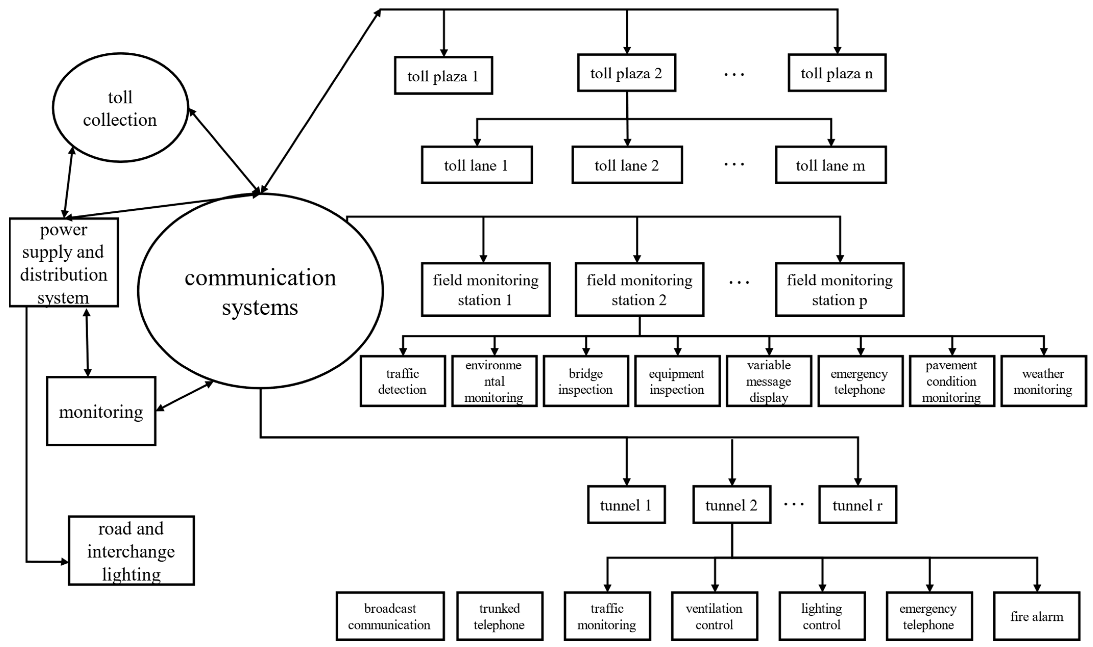
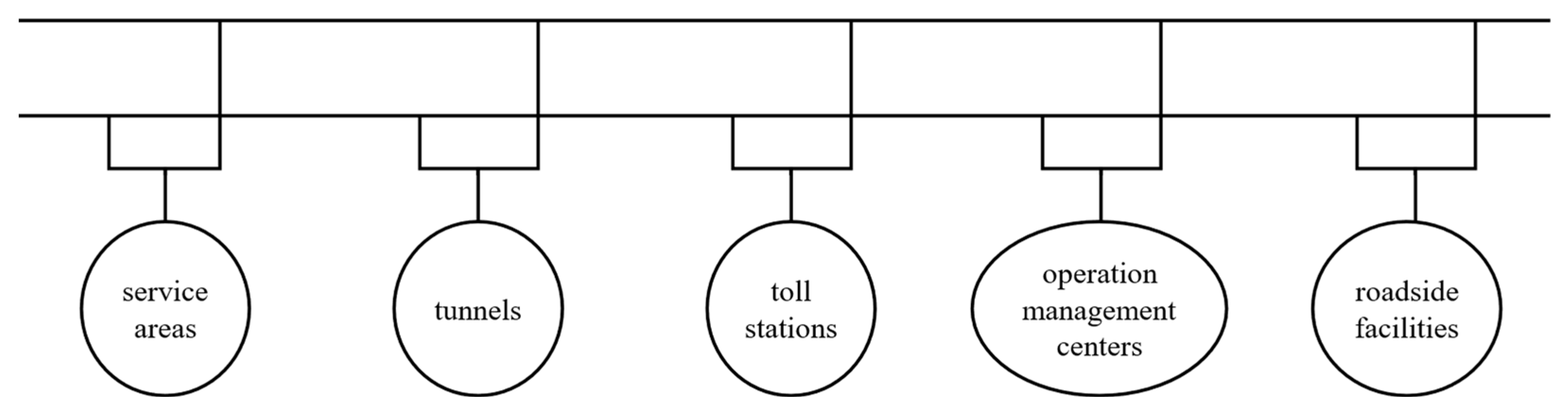
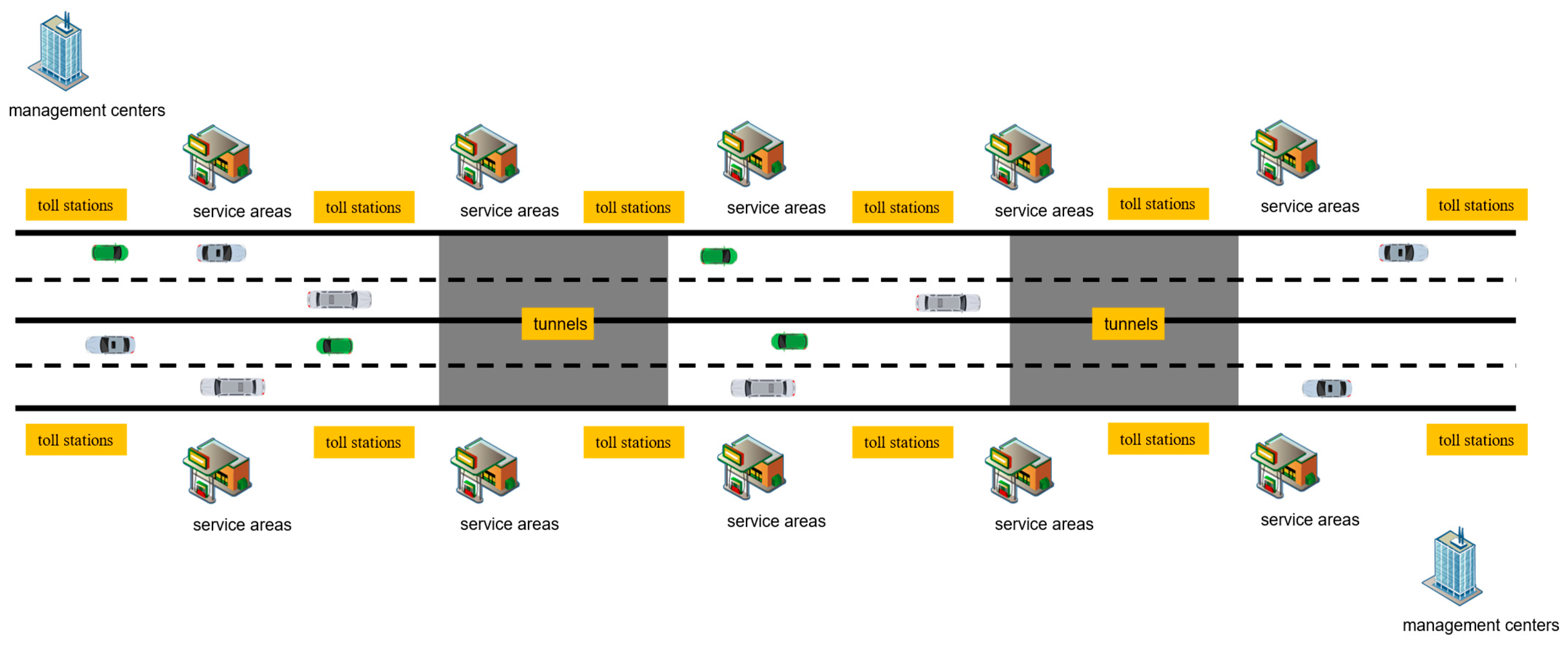
2. Energy Consumption Model for Highway Operations

The power facilities and equipment along highways are integral to transportation infrastructure and serve as primary tools for advancing the digitalization and intelligence of highways. These facilities form a comprehensive system grounded in electronic, electrical, control, communication, mechanical, and traffic engineering technologies. They include subsystems such as monitoring, tolling, communication, lighting, power distribution, and tunnel electromechanical systems, which are interconnected via communication networks [19], as shown in Figure 1.

Based on operational management functions, highway power facilities in China can be categorized into six systems: monitoring, tolling, communication, lighting, power distribution, and tunnel lighting/ventilation systems [20].

These energy units are distributed across various service scenarios, including service areas, tunnels, toll stations, operation management centers, and roadside facilities. For ease of calculation and analysis, the total energy consumption of highway operations can be represented as the aggregate energy demand across these five scenarios, as shown in Figure 2.

The model for measuring infrastructure energy consumption is expressed as follows:

$$E=E_S+E_U+E_T+E_O+E_A$$

(1)

where $E$ represents the total energy consumption (kWh); $E_S$, $E_U$, $E_T$, $E_O$, and $E_A$ denote the energy consumed by service areas, tunnels, toll stations, operation management centers, and roadside facilities, respectively.

2.1. Energy Consumption in Service Areas

Energy consumption in service and parking areas primarily includes lighting, restaurant electricity and gas usage, and power for charging stations. Given the diverse energy-consuming equipment, the consumption is calculated using a general comparative approach:

$$E_S=T_s\times \left({\sum }_{i=1}^n{q}_i^1+{\sum }_{j=1}^m{q}_j^2\right)$$

(2)

Here, $T_s$ represents the operating hours (h); $q_i^1$ and $q_j^2$ denote the daily energy consumption of the $i$-th service area and $j$-th parking area (kWh/24 h), respectively; $n$ and $m$ correspond to the total numbers of service areas and parking areas.

2.2. Energy Consumption in Tunnels

Tunnels rely on ventilation, lighting, monitoring, and communication systems to ensure safe transportation. As outlined in reference standards [21], tunnel energy consumption encompasses both the equipment within the tunnel and that located at its entrances.

$$E_T={\sum }_{h=1}^n\left({\displaystyle \frac{P_{h1}{T}_{h1}{L}_H}{L_{h1}}}+n_1{n}_H{P}_{h2}{T}_{h2}\right)$$

(3)

Here, $P_{h1}$ represents the rated power of internal equipment (kW); $T_{h1}$ is the spacing between equipment (m); $T_{h1}$ also denotes the operating time of internal equipment (h);$L_H$ is the total tunnel length (m); $n_1$ is the number of entrance equipment; $n_H$ is the number of tunnels; $P_{h2}$ and $T_{h2}$ are the rated power (kW) and operating time (h) of entrance equipment.

2.3. Energy Consumption at Toll Stations

Energy consumption in toll stations includes power for toll systems, monitoring systems, lighting, and management offices. The formula is as follows [22]:

$$E_T=P_{t1}{T}_{t1}{n}_t$$

(4)

where $P_{t1}$ is the rated power of toll station units (kW); $T_{t1}$ represents the operating time (h); $n_t$ denotes the total number of toll stations.

2.4. Energy Consumption in Operation Management Centers

Operation management centers consume energy through three primary components: equipment energy consumption [23], daily staff energy usage, and energy for maintenance and emergency response vehicles. The formula is as follows:

$$E_O=\left({\sum }_{i=1}^n{n}_{oi}\times P_i\times t_i\times T_o/1000+P_o\times w_o\times 12\right)$$

(5)

where $E_O$ is the energy consumption during $T_o$ hours (kWh); $n_{oi}$, $P_i$, and $t_i$ are the number, power (W), and average daily operating time (h) of equipment; $P_o$ and $w_o$ are the number of staff and average daily electricity consumption per person (kWh).

2.5. Energy Consumption of Roadside Facilities

Key energy-consuming devices along highways include vehicle detectors and emergency telephones. Based on monitoring and communication needs [22], energy consumption is calculated as follows:

$$E_A=T_a\left(L_r-1\right)\left(2P_d+P_c\right)$$

(6)

where $L_r$ is the highway length (km); $P_c$ and $P_d$ are the power of monitoring devices (kW) and emergency telephones (kW); $T_a$ is the operating time (h).

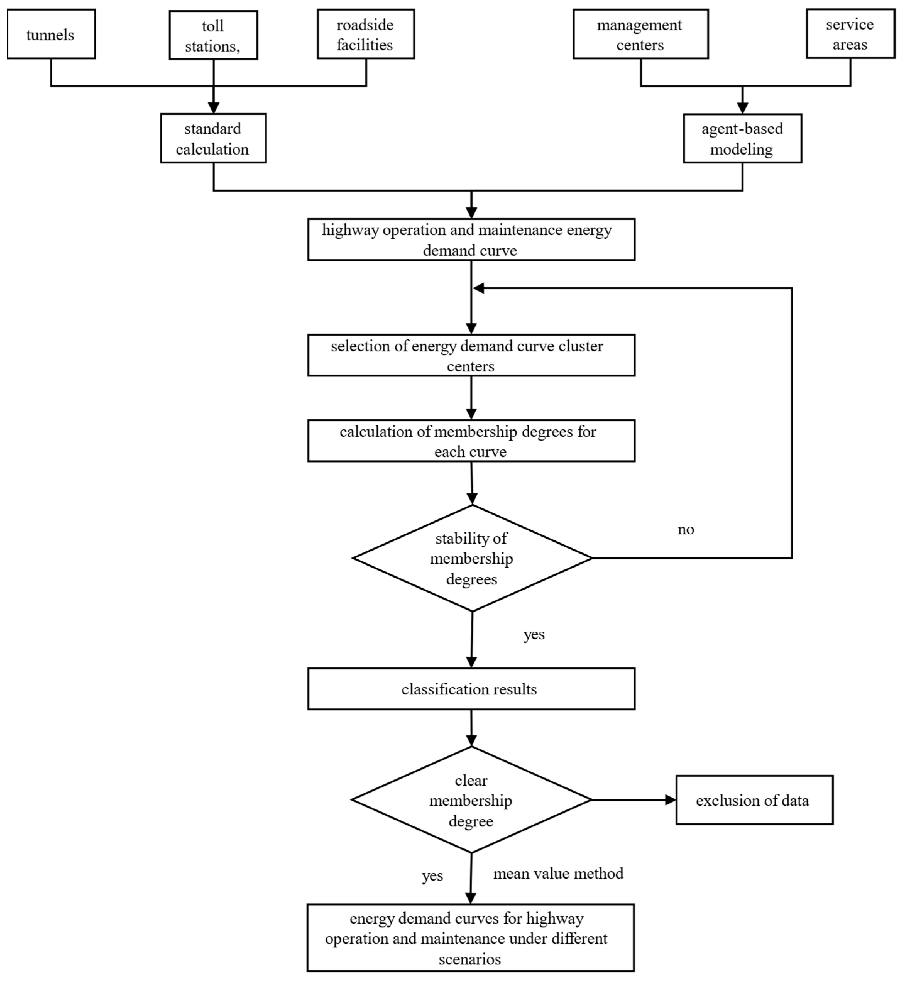
3. Energy Demand Curve Calculation

3.1. Energy Usage Scenarios

The calculation of energy demand scenarios for highways can be categorized into two types: those related to human activities and those unrelated. Tunnels, toll stations, and roadside equipment exhibit lower correlations with human activities, and thus their energy consumption can be computed using meteorological data and consumption characteristics, based on standard summation procedures [22,24]. Conversely, service areas and operation management centers are highly influenced by human activities, and energy demand forecasting is conducted using agent-based modeling (ABM), based on comprehensive activity characteristics [12]. The energy demand curve calculation for highway operations integrates both methods, as shown in Figure 3.

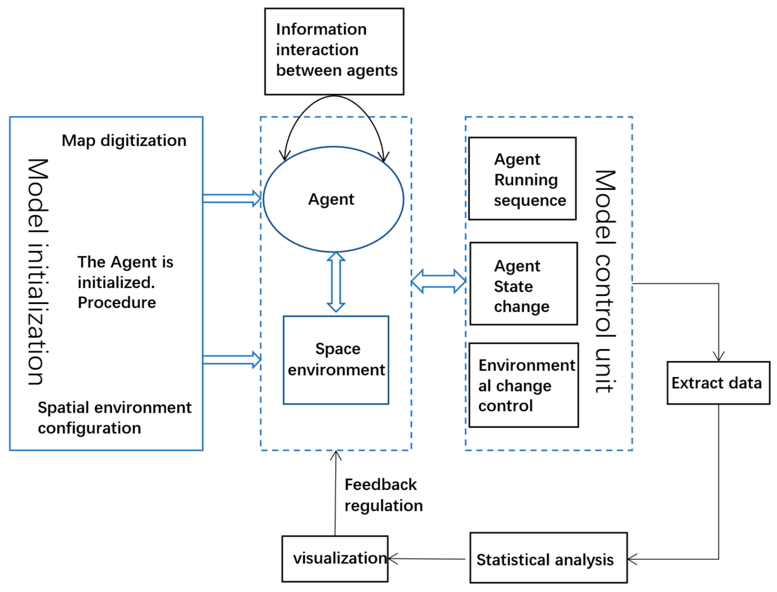
3.2. Agent-Based Modeling (ABM)

Agent-based modeling (ABM) is a simulation technique that constructs models comprised of multiple interacting agents to forecast energy consumption in buildings [12]. In the context of energy forecasting for buildings, each agent can represent a room, equipment, or user within a building. Each agent makes decisions based on specific rules and interacts with its environment and other agents. Agents gather information by perceiving environmental conditions and communicating with others. Based on this information, each agent can independently decide actions such as adjusting temperature settings, controlling equipment use, or changing behaviors.

In building energy demand forecasting using ABM, various influencing factors, such as temperature, humidity, foot traffic, and equipment usage, are considered. Agents can adjust their energy usage behavior based on environmental conditions and the behavior of other agents. For example, when the temperature rises, an agent may decide to lower the air conditioning temperature or turn off certain devices to reduce energy consumption. Interactions between agents are facilitated through information exchange and feedback mechanisms. For instance, one agent can monitor the surrounding temperature and humidity through sensors and pass this information to other agents, which may adjust their behavior, such as modifying heating system operations or activating ventilation.

ABM presents a degree of complexity in energy demand forecasting due to the interactions and decision-making processes between agents. By simulating the behavior and interactions of agents, a more accurate prediction of energy consumption can be made, along with an evaluation of the impact of various strategies on energy use.

The architecture of the ABM model is shown in Figure 4.

The modeling steps for service area agents are as follows:

• Defining Agent Types

Identify the types of agents in the system and their characteristics. Each vehicle’s arrival may increase the energy consumption of the service area, such as refueling and charging; drivers and passengers use the facilities of the service area, such as restrooms, restaurants, and supermarkets; staff operate facilities such as gas stations, restaurants, stores, and maintenance.

2.

Defining the Environment

The environment is the backdrop for agent interactions. It includes service facilities related to people, such as restrooms, catering departments, and supermarkets; service facilities related to vehicles, such as parking lots and charging stations; and other ancillary facilities, including offices, power distribution rooms, and waste treatment facilities.

3.

Defining Agent Behaviors

Define decision-making rules and behavioral patterns for each type of agent. For example, vehicles arrive at the service area at a certain probability at a specific time point, stay for a period, and then leave; drivers and passengers use different service area facilities and consume energy; staff operate facilities during specific time periods, affecting energy consumption.

4.

Establishing the Energy Consumption Model

Collect data related to energy consumption, including the energy efficiency ratios of equipment, the usage duration and load curves of each agent, and building characteristics. Additionally, external factors such as weather conditions and human traffic can be considered to assess their impact on energy consumption, thereby constructing a more accurate energy consumption model.

5.

Simulation and Modeling

Deploy the established energy consumption model into a simulated environment for operation. At each time point in the simulation, agents make decisions based on established rules and interaction mechanisms and interact with the environment and other agents. Simulations are typically run multiple times to account for the randomness of different traffic flows and behavioral patterns.

3.3. Fuzzy C-Means (FCM) Algorithm

The operational energy demand for a specific section of a highway includes energy consumption data from different types of vehicles under various conditions, as well as service energy consumption in different scenarios. Simple hard clustering methods, such as the K-means algorithm, may attempt to partition this data into discrete clusters—for instance, energy consumption by passenger cars in sunny weather, by trucks in rainy weather, or by mixed traffic under varied conditions. However, in real-world scenarios, energy consumption patterns are continuous, rather than discrete. Therefore, traditional hard clustering methods, such as K-means, which force each data point to belong to only one cluster, may overlook important information when handling actual data.

In the context of highway operation and maintenance energy demand classification, the FCM algorithm [12] assigns each energy usage scenario to different clusters based on membership degrees (similarities), represented as feature vectors for each scenario. The membership degree is determined by the distance between data points and the cluster center, with values ranging from 0 to 1. Higher values signify a closer proximity to the cluster center. This approach not only better captures the fuzziness and uncertainty inherent in the data but also permits data points to belong to multiple clusters, thereby more effectively representing the complex relationships within the data [25,26].

The objective function of the Fuzzy C-Means (FCM) algorithm is expressed as follows:

$$J\left(U,U^{\prime }\right)={\sum }_{n=1}^N{\sum }_{c=1}^C{l}_{n,c}^2{u}_{n,c}^2$$

(7)

Here, $l_{n,c}^2$ denotes the distance between the $n$-th sample and the $c$-th cluster center; $U$ is the membership matrix, with $u_{n,c}^2$ indicating the corresponding membership degree; $U^{\prime }$ is the cluster center matrix; and $c$ refers to the number of clusters.

For this study, the value of $c$ is determined by the number of classified scenarios, such as routine baseline scenarios, holidays, emergency events, and extreme weather disturbances. This section uses the FCM algorithm to filter the highway operation and maintenance energy demand across different scenarios, using membership degrees to eliminate anomalous energy load data.

The total energy usage can be expressed as follows:

$$V={\left[v_1, \dots , v_n, \dots , v_N\right]}^{\prime }$$

(8)

$$v_n=[v_{n,1}, v_{n,2}, \dots , v_{n,t}, \dots , v_{n,24}, v_{n,25}, v_{n,26}]$$

(9)

Here, $N$ denotes the total number of samples, and $v_n$ represents the energy load and highway information for the $n$-th day; $v_{n,t}$ is the energy consumption during the $t$-th hour of the $n$-th day; $v_{n,25}$ is the average traffic volume for the $n$-th day; and $v_{n,26}$ is the average precipitation for the $n$-th day.

FCM Algorithm Steps:

6.

Initialize the membership degree matrix $U^{\left(0\right)}$.

7.

Calculate the cluster center $U^{\prime }$ and membership matrix $U$ during the $d$-th iteration:

$$U_n^{{\left(0\right)}^{\prime }}={\displaystyle \frac{\sum _{n=1}^N{\left[u_{n,c}^{\left(d-1\right)}\right]}^p{v}_n}{\sum _{n=1}^N{\left[u_{n,c}^{\left(d-1\right)}\right]}^p}}$$

(10)

$$u_{n,c}={\displaystyle \frac{1}{\sum _{k=1}^C{\left[\frac{l_{n,c}}{l_{n,k}}\right]}^{\frac{2}{m-1}}}}$$

(11)

where $p$ is the fuzzy exponent.

8.

Compute the objective function:

$$J^{\left(d\right)} [U^{\left(d\right)}{U}^{{\left(d\right)}^{\prime }}]={\sum }_{n=1}^N{\sum }_{c=1}^C{\left[l_{n,c}^{\left(d\right)}\right]}^2{\left[u_{n,c}^{\left(d\right)}\right]}^2$$

(12)

9.

Should the difference in membership degrees between two iterations fall below the threshold $K_u$, the sample is assigned to a classification. If this condition is not satisfied, the process returns to step 2 to continue the iteration.

10.

Once stable classification results are achieved, the membership degree of each sample is evaluated to determine if it exceeds the threshold T. If the membership degree is below this threshold, the sample is classified as noisy data and excluded from the energy demand curve calculation.

After performing FCM clustering on the data, the energy demand curve for each scenario $c$ is calculated by averaging the hourly energy load for each cluster, as follows:

$$y_t^c={\displaystyle \frac{\sum _{n=1}^N{v}_{n,t}^c}{N}}$$

(13)

4. Case Study Analysis

To assess the effectiveness of the Fuzzy C-Means (FCM) algorithm in forecasting highway operation and maintenance energy demand, this study simulates highway operations under four distinct scenarios.

4.1. Simulation Scenarios

A highway network structure is defined, as illustrated in Figure 5. The highway is unidirectional, with a total length of 300 km, a design speed of 100 km/h, a roadbed width of 26 m, two long tunnels (each 3500 m in length), ten type II service areas, twelve toll stations, and two operation management centers. Based on traffic flow data from literature [1,27,28,29,30,31] and measured data from highways in Western China, the corresponding simulation scenarios are constructed, incorporating traffic flow and meteorological information.

The simulations are carried out for four scenarios: routine operation, major holidays, snowy weather, and extreme weather. The impact characteristics of these scenarios on highway operational energy demand are simulated, and the energy demand results are calculated using the methods described in Section 3, serving as input for the clustering model. The Fuzzy C-Means (FCM) clustering method partitions the data into four clusters, as presented in

Table 2. Study scenario-related features.

Scenario	Base Scenario	Disturbance Scenario 1	Disturbance Scenario 2	Disturbance Scenario 3
Time	0–24 h	0–24 h	0–24 h	0–24 h
Scenario Description	Good weather, no major traffic incidents, smooth road conditions	Mid-autumn holiday, peak travel period, road network service capacity under stress	Moderate snowfall in the study area, road network under stress	Heavy snowfall, snow accumulation, road closures, road network capacity under significant strain
Operating Conditions	Normal traffic conditions	High traffic volume	Snowy weather disruption	Severe weather disruption

. The clustering process utilized $c=4$, with an error threshold $K_u={10}^{-8}$, a maximum iteration count of 2000, and a membership threshold of $T=0.6$.

In this table, “Base Scenario” refers to normal operating conditions without significant disturbances, while the other scenarios simulate specific disturbances such as holidays, snow events, and extreme weather conditions. These scenarios are used to explore the variation in energy demand in the face of different operational challenges.

4.2. Operational Energy Demand of Highways Under Different Scenarios

As shown in Figure 6, the energy consumption proportions of various service energy usage scenarios in the highway operation and maintenance system vary significantly under different scenarios. In the baseline scenario, energy consumption by roadside facilities and service areas constitutes 31% and 28%, respectively. Notable energy consumption is also observed in tunnels and toll stations, while the operation management centers exhibit the lowest consumption, accounting for just 5%. In Disturbance Scenario 1, due to the increased vehicle flow during holidays, the energy consumption proportion of service areas rises significantly to 50%. The energy consumption proportions of other service scenarios decrease accordingly, especially for operation management centers, where energy consumption drops to 3%. In Disturbance Scenario 2, the energy consumption proportion of roadside facilities is the highest at 34%, with tunnel energy consumption increasing significantly to 25%. The energy consumption proportions of service areas, toll stations, and operation management centers are comparatively low. In Disturbance Scenario 3, the energy consumption of roadside facilities continues to rise, reaching 36%. Tunnel energy consumption is also high at 26%. The energy consumption of service areas and toll stations is relatively low. Due to the snow accumulation requiring emergency rescue efforts from operation management centers, their energy consumption proportion slightly increases to 6%.

4.2.1. Total Energy Consumption Profile in the Baseline Scenario

Figure 7 illustrates that the total energy consumption curve in the baseline scenario exhibits a positive correlation with vehicle traffic. The trend of traffic flow changes mirrors that of the total energy consumption curve. Due to low traffic volume and facility usage in the early morning, there is a trough in energy consumption between 6:00 and 8:00. From 10:00 to 14:00, during the peak period of daily travel, the number of vehicles entering service areas gradually increases, leading to frequent activities and a local peak in total energy consumption, which rises significantly to around 9940 kWh. Between 14:00 and 17:00, with fewer vehicles entering the service areas, energy consumption decreases again. From 18:00 to the next morning at 6:00, lighting systems across various service scenarios are turned on, causing energy consumption to rise and stabilize between 6000 kWh and 8000 kWh.

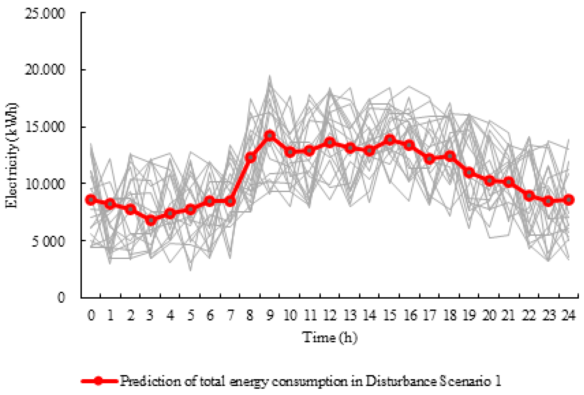
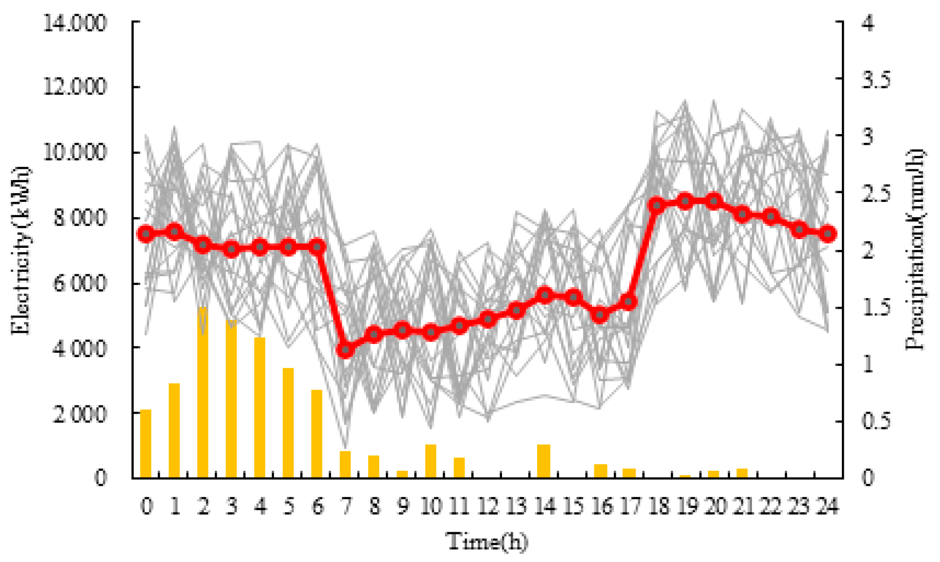
4.2.2. Total Energy Consumption Curve in Disturbance Scenario 1

As shown in Figure 8, during holidays, due to the significant increase in vehicles entering service areas, energy consumption from 8:00 to 18:00 remains at a high level, fluctuating between 12,000 kWh and 14,000 kWh. Compared to the baseline scenario, the peak energy consumption period is extended from 8:00 to 17:00, with total energy consumption increasing by 30.2% on average. As a result, the proportion of energy consumption from service areas relative to total energy usage increases by 22%, as shown in Figure 6a,b.

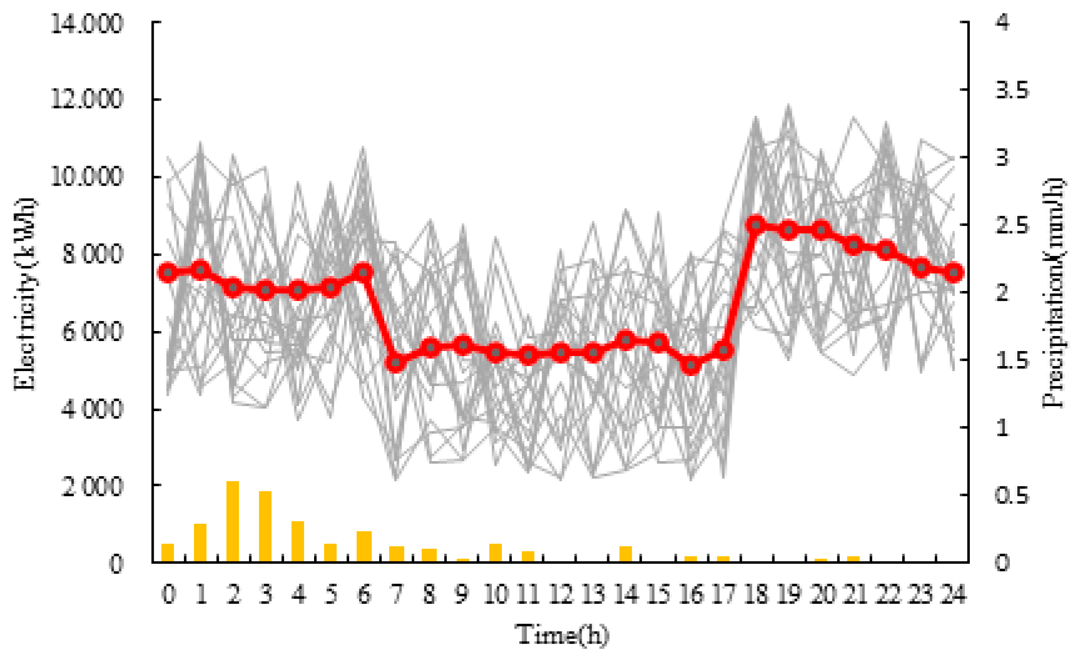
4.2.3. Total Energy Consumption Curve in Disturbance Scenario 2

As shown in Figure 6 and Figure 9, the energy demand from service areas is highly influenced by weather and foot traffic. During a moderate snowstorm, although the highway remains passable, the number of vehicles decreases significantly compared to the baseline scenario. The average energy consumption in service areas decreases by 30.9%, and its proportion of total energy consumption drops to 14.7%. Compared to the baseline scenario from 10:00 to 14:00, energy consumption sharply declines, with total energy usage per hour decreasing by 39.1% on average. From 16:00 to 18:00, energy consumption gradually increases due to the activation of lighting systems in roadside facilities.

4.2.4. Total Energy Consumption Curve in Disturbance Scenario 3

During heavy snowfall, snow accumulation begins to block the highway at 7:00, preventing normal traffic flow. As shown in Figure 10, from 8:00 to 11:00, during the emergency road rescue period, service areas only maintain lighting, heating, and other essential infrastructure energy usage, with no additional vehicles entering for refueling or charging. Therefore, total energy consumption significantly drops from 7:00 to 8:00. Overall, energy consumption remains at a low level, fluctuating between 4000 kWh and 6000 kWh. After the emergency rescue ends and normal traffic resumes, energy consumption rises again from 18:00 to 22:00, fluctuating between 8000 kWh and 10,000 kWh.

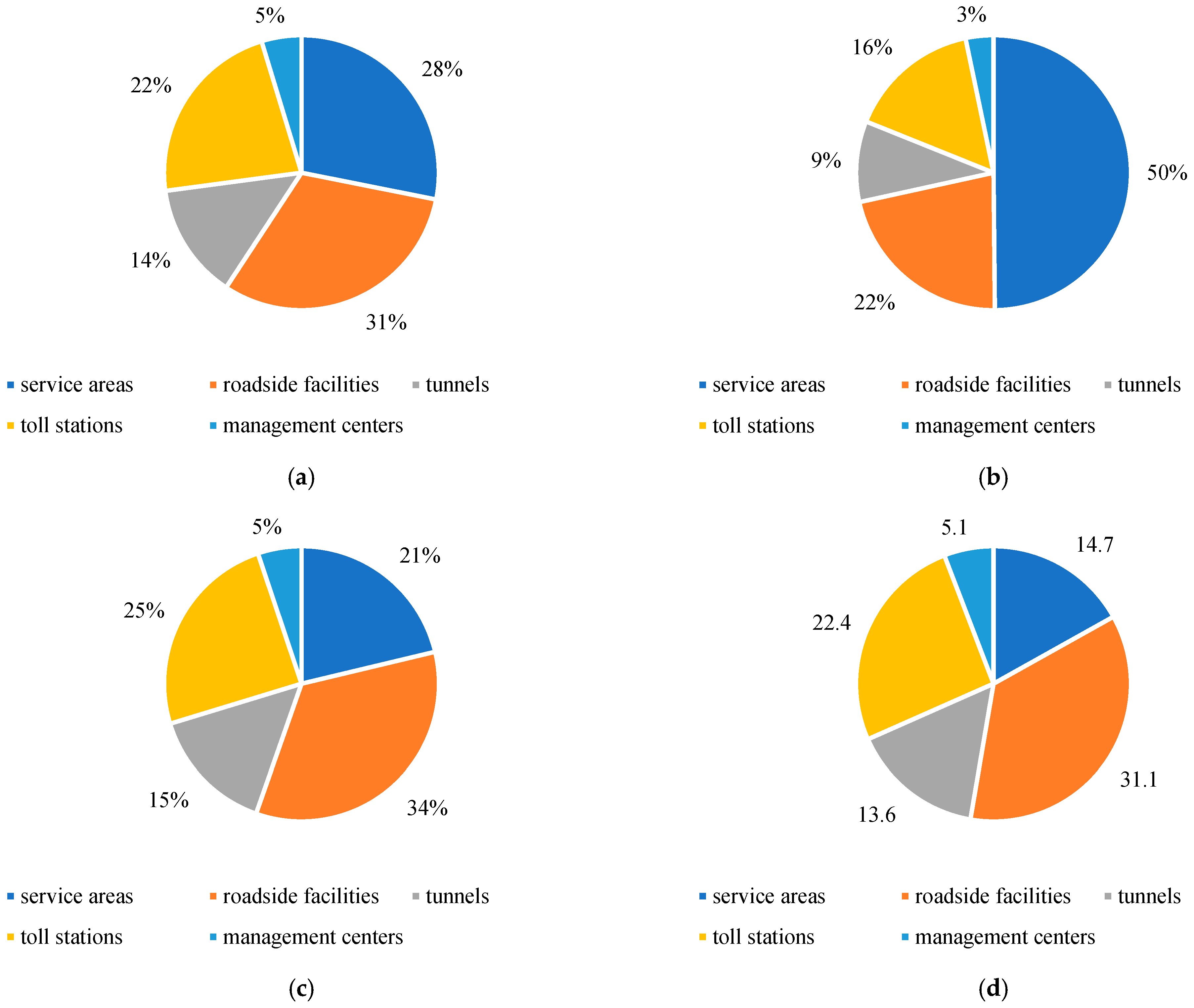
4.3. Energy Consumption Comparison Across Different Scenarios

As presented in

Table 3. Total daily electricity consumption comparison.

Scenario	Total Daily Energy (kWh)	Relative to Baseline (%)
Baseline Scenario	185,424.3	100.0
Disturbance Scenario 1	265,692.5	143.2
Disturbance Scenario 2	169,259.3	91.2
Disturbance Scenario 3	161,197.8	86.9

and

Table 4. Peak daily electricity consumption comparison.

Scenario	Peak Daily Energy (kWh)	Relative to Baseline (%)
Baseline Scenario	21,818.8	100.0
Disturbance Scenario 1	26,173.1	143.8
Disturbance Scenario 2	19,064.6	88.3
Disturbance Scenario 3	18,781.2	85.5

, in Disturbance Scenario 1, the increase in vehicle traffic during holidays leads to a higher electricity demand. Specifically, total daily energy consumption rises by 143.2% compared to the baseline scenario, while peak power demand increases by 43.8%. In Disturbance Scenario 2, despite the increase in heating demand due to snow, the reduction in vehicle flow leads to a decrease in total energy consumption by 8.8%, with peak demand dropping by 11.7%. In Disturbance Scenario 3, while energy demand from operational sites increases due to snow accumulation, the significant reduction in vehicle flow results in a decrease in service energy consumption. As a result, total energy consumption is slightly lower than in the snow-free scenario, dropping by 13.1%, and peak power demand decreases by 14.5%.

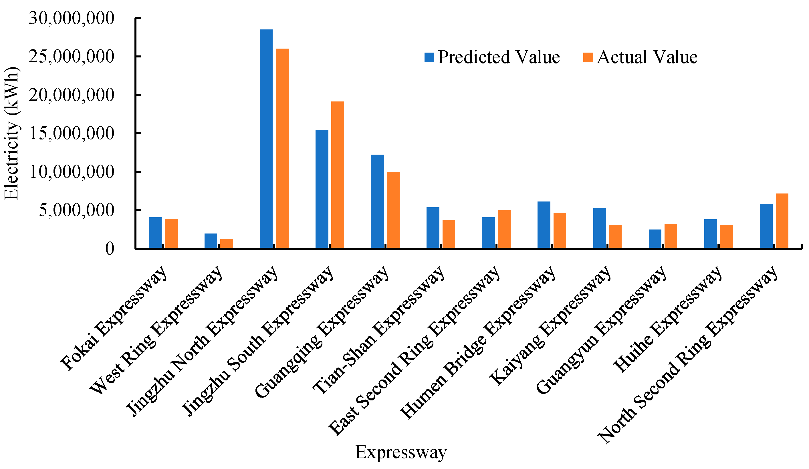
4.4. Model Validation

To further assess the accuracy of the developed model, this study utilized energy consumption data from 12 cities [32,33] to conduct a comprehensive validation analysis of the highway energy consumption model. In the validation process, the actual parameter values collected were first input into the model to predict the total energy consumption for each highway. These predicted values were then compared with the observed values to evaluate the model’s predictive accuracy. The results of this validation are presented in Figure 11 and

Table 5. Actual and predicted highway energy consumption statistics.

Type	Predicted Value (kWh)	Actual Value (kWh)
Minimum	1,952,880	1,269,616.11
Maximum	28,479,500	28,479,500
Mean	7,916,622.91	7,708,363.18
Variance	7,575,607.35	8,088,179.79

, which clearly illustrate the comparison between predicted and actual values.

Using the Wilcoxon signed-rank test method with the above data, the calculated p-value for hypothesis testing is 0.30, which is far greater than the significance level of 0.05. Therefore, the predicted total energy consumption of the highway does not exhibit significant differences from the actual values, thus validating the accuracy of the highway energy consumption model. This validation step ensures the reliability and effectiveness of the model for practical applications.

5. Conclusions

Based on agent-based modeling and the FCM method, this study developed a dynamic energy demand forecasting model for highway operations and maintenance, calculating the energy demand curves for highway operations under regular conditions, major holidays, snowy weather, and extreme weather events. The model reflects the load characteristics of highway operational energy systems and the energy behaviors of agents under different scenarios. Finally, the model’s effectiveness and reliability were validated through case analysis, leading to the following conclusions:

During major holidays, the significant increase in highway traffic results in a sharp rise in energy demand. Total daily energy consumption and peak energy demand increased by 143.2% and 43.8%, respectively, compared to the baseline scenario. This substantial increase highlights the immense pressure on the energy supply system during peak holiday periods, necessitating effective planning and optimization to meet the surge in energy demand.

In contrast to holidays, snowy weather leads to a reduction in vehicle flow, resulting in a decrease of 8.8% in total energy consumption and 11.7% in peak demand. However, the increased heating load partially offsets this decline. This demonstrates the need for flexibility in energy demand forecasting and management strategies to accommodate the dual impacts of reduced vehicle flow and increased heating load under specific weather conditions.

In extreme weather conditions, such as heavy snowfall and road closures, highway operations are severely impacted, leading to a further reduction in energy demand. Total energy consumption and peak demand decreased by 13.1% and 14.5%, respectively. This phenomenon emphasizes the importance of incorporating the effects of weather on traffic flow and operational activities in energy demand forecasting models to ensure the stability and reliability of the energy supply system under extreme weather conditions.

The analysis results from this study highlight the dynamic variations in highway energy demand under different weather conditions. These findings are critical for formulating effective energy management strategies, optimizing energy supply systems, and improving the energy efficiency of highway operations when facing diverse weather challenges. Future research should further explore how these findings can be applied to practical energy scheduling and highway operation management practices to achieve more efficient and sustainable energy management.

References

1. Jia, L.; Shi, R.; Ji, L.; Wu, P. Research on integrated development strategy of road transportation and energy in China. Eng. Sci. 2022, 24, 163–172. [Google Scholar]
2. Shi, R.; Gao, Y.; Ning, J.; Tang, K.; Jia, L. Research on Highway Self-Consistent Energy System Planning with Uncertain Wind and Photovoltaic Power Output. Sustainability 2023, 15, 3166. [Google Scholar] [CrossRef]
3. Shi, R.; Ning, J.; Gao, Y.; Jia, L. Research on Optimal Scheduling Strategy of Highway Traffic Wind and Light Self-consistent Microgrid System with Hydrogen Energy Storage. J. Solar Energy 2023, 44, 513–521. [Google Scholar]
4. Yuan, M.; Mai, J.; Liu, X.; Shen, H.; Wang, J. Current Implementation and Development Countermeasures of Green Energy in China’s Highway Transportation. Sustainability 2023, 15, 3024. [Google Scholar] [CrossRef]
5. Wang, J.; Fu, L.; Shang, K.; Chen, G. Research on Short-term Energy Consumption Prediction Model of Highway Tunnel Operation based on CEEMDAN-SVR. Highw. Transp. Technol. 2023, 39, 145–152. [Google Scholar]
6. Fan, Q.; Li, M.; Sun, Z. Prediction and analysis of road energy consumption and emission in Guangdong Province based on COPERT model. Transp. Energy Conserv. Environ. Prot. 2022, 18, 40–44. [Google Scholar]
7. Jing, C. Study on Life Cycle Energy Consumption and Carbon Emission of Rural Roads in Inner Mongolia. Master’s Thesis, Chang’an University, Chang’an, China, 2019. [Google Scholar]
8. Cansiz, Ö.; Ünes, F.; Erginer, İ.; Taşar, B. Modeling of highways energy consumption with artificial intelligence and regression methods. Int. J. Environ. Sci. Technol. 2022, 19, 9741–9756. [Google Scholar] [CrossRef]
9. Wu, Q.; Chen, Y.; Li, C.; Shi, X. Carbon emission scenario prediction for highway construction projects. Front. Environ. Sci. 2024, 11, 1302220. [Google Scholar] [CrossRef]
10. Zhang, Y.; Kong, Y.; Quan, J.; Wang, Q.; Zhang, Y. Scenario analysis of energy consumption and related emissions in the transportation industry—A case study of Shaanxi Province. Environ. Sci. Pollut. Res. 2024, 31, 26052–26075. [Google Scholar] [CrossRef]
11. Ruan, F.; Zhang, W.; Qian, K.; Qian, X.; Wang, L. Simulation and verification of Human Behavioral Energy Consumption in Residential Buildings in Hot Summer and cold Winter Region based on DeST. Build. Energy Eff. 2017, 45, 1–6. [Google Scholar]
12. Wang, N.; Qu, C.; Yang, C.; Wang, J. Multi-energy load forecasting in Service Area based on agent Modeling and improved FCM. J. N. China Electr. Power Univ. (Nat. Sci. Ed.) 2024, 51, 67–75. [Google Scholar]
13. Alonso-Adame, A.; Farahbakhsh, S.; Van Meensel, J.; Marchand, F.; Van Passel, S. Factors to scale out innovative organic farming systems: A case study in Flanders region, Belgium. Agric. Syst. 2025, 224, 104219. [Google Scholar] [CrossRef]
14. Martin, G.; Allain, S.; Bergez, J.E.; Burger-Leenhardt, D.; Constantin, J.; Duru, M.; Hazard, L.; Lacombe, C.; Magda, D.; Magne, M.-A.; et al. How to address the sustainability transition of farming systems? A conceptual framework to organize research. Sustainability 2018, 10, 2083. [Google Scholar] [CrossRef]
15. Farahbakhsh, S.; Snellinx, S.; Mertens, A.; Belderbos, E.; Bourgeois, L.; Van Meensel, J. What’s stopping the waste-treatment industry from adopting emerging circular technologies? An agent-based model revealing drivers and barriers. Resour. Conserv. Recycl. 2023, 190, 106792. [Google Scholar] [CrossRef] [PubMed]
16. Kocabey Ciftci, P.; Unutmaz Durmusoglu, Z.D. A hybrid agent-based model integrated with a multi-stage learning-based fuzzy cognitive map. Kybernetes 2024, 53, 3685–3706. [Google Scholar] [CrossRef]
17. Bustamante, M.; Rillo, C.; Niang, I.; Baker, L.; Vidueira, P. Harvesting insights for transformation: Developing and testing a participatory food systems modeling framework in Southern Senegal’s poultry system. Agric. Syst. 2024, 217, 103941. [Google Scholar] [CrossRef]
18. Ahmad, S.; Jia, H.; Ashraf, A.; Yin, D.; Chen, Z.; Ahmed, R.; Israr, M. A Novel GIS-SWMM-ABM Approach for Flood Risk Assessment in Data-Scarce Urban Drainage Systems. Water 2024, 16, 1464. [Google Scholar] [CrossRef]
19. Li, X. On the application of Mechatronics Technology in Traffic engineering facilities. North Commun. 2014, 12, 104–106. [Google Scholar]
20. Liu, Z.; Tan, Y.; Xia, L.; Qiang, R.; Zhao, J. Energy supply status and demand analysis of highway transportation facilities. Highw. Transp. Sci. Technol. 2022, 39, 353–358. [Google Scholar]
21. Code for Design of Highway Tunnel Traffic Engineering. Available online: https://xxgk.mot.gov.cn/2020/jigou/glj/202006/t20200623_3312234.html (accessed on 17 February 2024).
22. Standard for Quality Inspection and Evaluation of Highway Engineering Volume II Electromechanical Engineering. 2020. Available online: https://xxgk.mot.gov.cn/2020/jigou/glj/202012/t20201230_3510057.html (accessed on 17 February 2024).
23. Zeng, Y. Analysis on Information Management in Expressway Operation Management. Guangdong Highw. Transp. 2010, 03, 80–84. [Google Scholar]
24. Yang, J.; Miao, Z. Energy Saving Calculation and Analysis of expressway during operation. Transp. Sci. Technol. 2018, 03, 173–176. [Google Scholar]
25. Bezdek, J.; Ehrlich, R.; Full, W. FCM: The fuzzy c-means clustering algorithm. Comput. Geosci. 1984, 10, 191–203. [Google Scholar] [CrossRef]
26. Venu, D. PSNR Based Evaluation of Spatial Gaussian Kernels For FCM Algorithm with Mean and Median Filtering Based Denoising for MRI Segmentation. IJFANS Int. J. Food Nutr. Sci. 2023, 12, 928–939. [Google Scholar]
27. Verma, H.; Verma, D.; Tiwari, P. A population based hybrid FCM-PSO algorithm for clustering analysis and segmentation of brain image. Expert Syst. Appl. 2021, 167, 114121. [Google Scholar] [CrossRef]
28. Yuan, G.; Jiao, L.; Rong, X.; Yang, Z.; Kong, X. Practice research on passive ultra-low energy buildings in expressway service areas. Build. Energy Eff. 2019, 47, 82–87. [Google Scholar]
29. Tian, T. Optimal Allocation of Highway Natural Disaster Emergency Treatment Equipment in Xinjiang. Master’s Thesis, Xinjiang University, Urumqi, China, 2019. [Google Scholar]
30. Gong, D. Study on the Influence of Rain and Snow on Urban Road Traffic Operation. Master’s Thesis, Beijing Jiaotong University, Beijing, China, 2016. [Google Scholar]
31. Zhou, F.; Wang, G.; Wang, L.; Liu, D.; Yi, Q. Snow and ice detection and early warning on expressways in cold regions. Transp. Syst. Eng. Inf. 2013, 13, 178–182+188. [Google Scholar]
32. Li, D. Research on Energy Consumption Analysis Method of Expressway Operation Period. Doctoral Thesis, South China University of Technology, Guangzhou, China, 2021. [Google Scholar]
33. Tang, K. Research on Analysis and Calculation Method of Energy Consumption Level in Expressway Operation Period. Master’s Thesis, Chang’an University, Chang’an, China, 2013. [Google Scholar]
Figure 1. Classification of energy-using units.
Sustainability 17 01929 g001
Figure 2. Energy usage scenario of highway operation and maintenance service.
Sustainability 17 01929 g002
Figure 3. Calculation process of the energy demand curve for highway operation and maintenance in different scenarios.
Sustainability 17 01929 g003
Figure 4. Architecture of the ABM.
Sustainability 17 01929 g004
Figure 5. Highway network structure.
Sustainability 17 01929 g005
Figure 6. The proportion of each service energy usage scenario to the total energy usage. (a) baseline scenario; (b) Disturbance Scenario 1; (c) Disturbance Scenario 2; (d) Disturbance Scenario 3.
Sustainability 17 01929 g006
Figure 7. Energy requirements in basic scenarios.
Sustainability 17 01929 g007
Figure 8. Energy requirements in Disturbance Scenario 1.
Sustainability 17 01929 g008
Figure 9. Energy requirements in Disturbance Scenario 2.
Sustainability 17 01929 g009
Figure 10. Energy requirements in Disturbance Scenario 3.
Sustainability 17 01929 g010
Figure 11. Comparison between actual and predicted energy consumption of highway.
Sustainability 17 01929 g011