Article

Machine Learning to Forecast Airborne Parietaria Pollen in the North-West of the Iberian Peninsula

by
Gonzalo Astray
1,*,
Rubén Amigo Fernández
2,
María Fernández-González
2,
Duarte A. Dias-Lorenzo
2,
Guillermo Guada
2 and
Francisco Javier Rodríguez-Rajo
2
1
Departamento de Química Física, Facultade de Ciencias, Universidade de Vigo, 32004 Ourense, Spain
2
Departamento de Bioloxía Vexetal e Ciencias do Solo, Facultade de Ciencias, Universidade de Vigo, 32004 Ourense, Spain
*
Author to whom correspondence should be addressed.
Sustainability 2025, 17(4), 1528; https://doi.org/10.3390/su17041528
Submission received: 28 November 2024 / Revised: 8 January 2025 / Accepted: 6 February 2025 / Published: 12 February 2025
(This article belongs to the Section Pollution Prevention, Mitigation and Sustainability)

Abstract

:
Pollen forecasting models are helpful tools to predict environmental processes and allergenic risk events. Parietaria belongs to the Urticaceae family, and due to its high-level pollen production, is responsible for many cases of severe pollinosis reactions. This research aims to develop different machine learning models such as the random forest—RF, support vector machine—SVM, and artificial neural network—ANN models, to predict Parietaria pollen concentrations in the atmosphere of northwest Spain using 24 years of data from 1999 to 2022. The results obtained show an increase in the duration and intensity of the Parietaria main pollen season in the Mediterranean region (Ourense). Machine learning models exhibited their capacity to forecast Parietaria pollen concentrations at one, two, and three days ahead. The best selected models presented high correlation coefficients between 0.713 and 0.859, with root mean squared errors between 5.55 and 7.66 pollen grains·m−3 for the testing phase. The models developed could be improved by increasing the number of years, studying other hyperparameter ranges, or analyzing different data distributions.

1. Introduction

Across all of the United Nations’ Sustainable Development Goals (SDGs), the monitoring of airborne pollen is included in SDG 3 Health and Wellbeing, SDG 11 Sustainable cities and Communities, SDG 13 Climate Action, and SDG 15 Life on Land [1]. These Sustainable Development Goals were signed in 2015 in a global agreement by the 193 member states of the United Nations to end poverty, protect the habitability of the planet, and ensure peace and prosperity [2]. The global prevalence and burden of respiratory diseases already affects more than 300 million people worldwide, and due to detection difficulties, such as cost complexity [3] or inability to access medical treatment [4], airborne pollen monitoring has become a critical part of providing local information to prevent and sustainably manage pollen exposure [5].
Parietaria is a genus of herbs that belongs to the Urticaceae family [6]. This family includes a group of some 45 genera and more than a thousand species of herbaceous plants and small bushes. The most common genera in this family in Spain are Parietaria and Urtica. The genus Parietaria includes the species Parietaria officinales, Parietaria judaica, and Parietaria cretica. On the other hand, the genus Urtica includes Urtica dioica and Urtica membranacea [7].
Due to the great similarity of the pollen of these two genera under the light microscope, as well as the similarity of their pollination period, the identification of these two genera is a difficult challenge [8]. For this reason, plants belonging to the genus Urtica are included in the pollen type Parietaria with the exception of Urtica membranacea, which can be distinguished under the light microscope [9].
This family is important because it is one of the most abundant pollen types in the Iberian Peninsula, representing between 8 and 13% of the total annual pollen counts in Spain [10]. Its high allergenic capacity is mainly due to the presence of Parietaria pollen, as the allergenic capacity of the genus Urtica is relatively low [11]. In Spain, the sensitization rates to Parietaria pollen range from 25 to 50% [12]. Considering the increase in the prevalence of allergies in Europe, especially in the last decade [13], it is important to develop models to predict the airborne pollen concentration and to establish preventive measures to protect the allergic community, particularly on critical days during the flowering period [14].
The REA (Spanish Aerobiology Network) has established four pollen groups of pollen classification concentrations of different taxa. In each group, four pollen categories were defined, which indicate the risk of the allergic population developing any symptoms. In the case of Urticaceae family, it belongs to group 1, and the categories established by the REA are: No risk: < 1   grains · m 3 ; Low risk: 1 15   grains · m 3 ; Moderate risk: 16 30   grains · m 3 ; and High risk: > 30   grains · m 3 [15].
Plants of the Urticaceae family are predominantly herbaceous, with one of their main characteristics being the presence of stinging hairs [16]. The genus Parietaria includes both annual and perennial herbs, with alternate, petiolate, and entire leaves [9], oval to lanceolate in shape [11]. The inflorescences are grouped in axillary fascicles of more than 5 mm, consisting of clusters of 3 to 10 flowers [6]. This type of plant usually grows on nitrogen-rich soils, and can also grow on walls, rocks, or fissures [9].
The flowering period of Parietaria covers practically the whole year, although the spring and summer months, specifically May, June, and July, are the most relevant [11]. The pollen grain is small, with an average size between 11 and 18 µm [17], spheroidal in shape, and trizonoporate [6], sometimes tetrazonoporate, isopolar and radiosymmetric, the openings are simple circular pore [11] (Figure 1).
Parietaria pollen in the atmosphere is of crucial importance in matters related to public health and environmental management. Due to this, it is easily understandable that the ability to predict the pollen concentration in the atmosphere, one, two, or three days ahead could allow those individuals susceptible to allergic reactions to take measures to avoid activities outdoors at critical moments of pollen concentration. This could reduce the incidence of allergic crises and have a favourable impact on the population’s health.
These critical situations, as well as the rest of the pollen season, could be analyzed/predicted using different kinds of models. According to Zhong et al. (2024) [18], there is a large amount of previous works where traditional statistical models, time series models such as ARIMA or dynamic regression, have been widely used [19,20,21,22,23,24]. On the other hand, there is currently a great development of models based on machine learning taking place that could allow for the modelling of the behaviour of pollen in the atmosphere. Machine learning models are optimized to achieve the best predictions within the feature space of the database used for training; however, despite this good performance, these types of models can be described as black boxes, because it is difficult to interpret what exactly has happened to arrive at the results produced using the input data [25]. Among the most used models, random forests, support vector machines, or artificial neural networks can be listed. Machine learning models have several advantages over traditional regression models, one of them and probably the most notable being the ability they have to fit the data without the need for prior assumptions [26].
In view of the aforementioned information, the objective of this research is to forecast airborne Parietaria pollen one, two, and three days ahead, using machine learning approaches based on the random forest, support vector machine, and artificial neural network models.

2. Materials and Methods

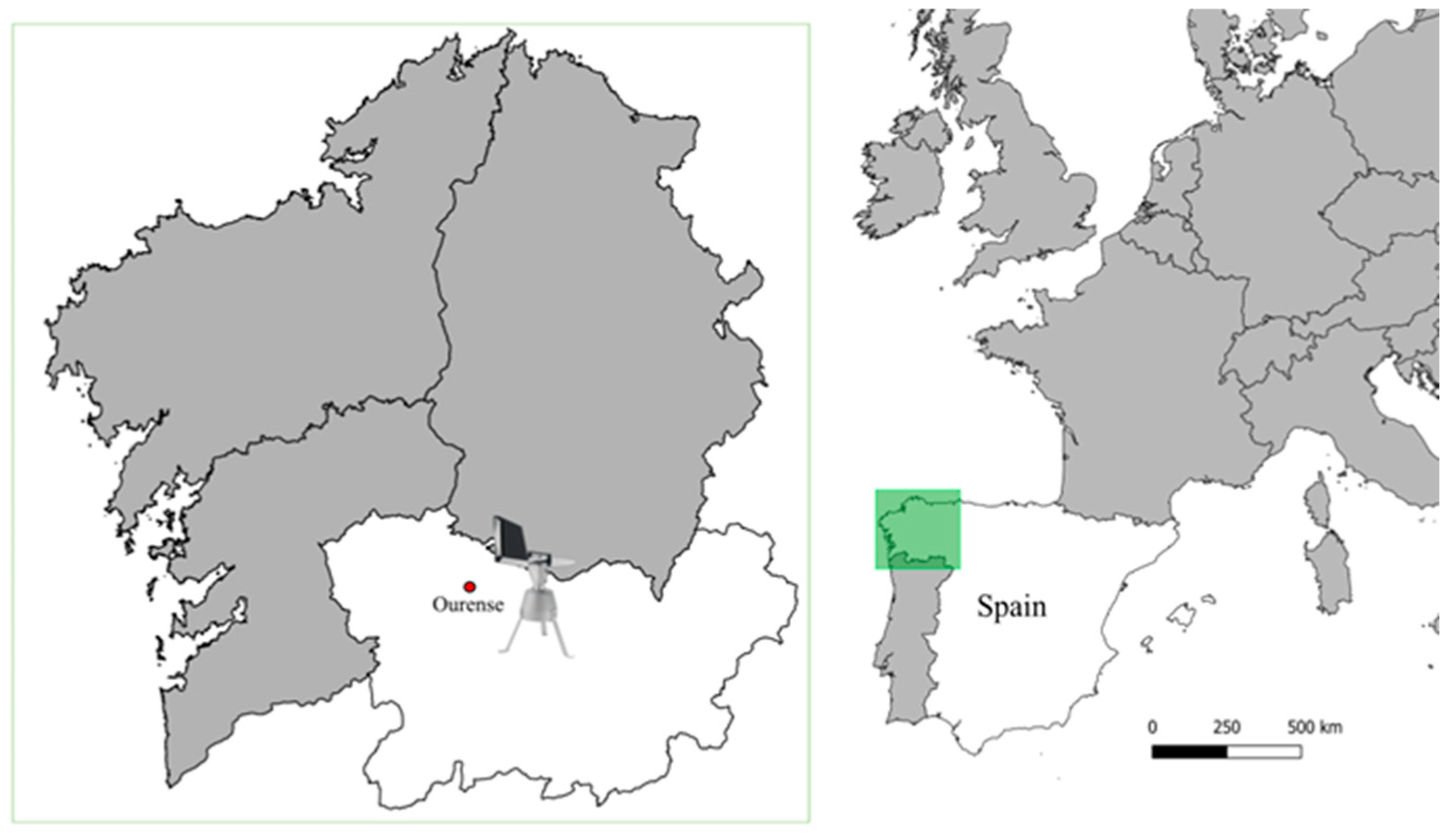
2.1. Location, Study Area, and Climatic Characterization of the Study Area

This study was conducted in the city of Ourense (42°20′ N 7°52′ W), located in the South-East of Galicia (Figure 2). The Galician territory is located between 42 and 44° N and 7 and 10° W, which gives an oceanic climate with abundant rainfall. Rainfall is evenly distributed throughout the year [27].
The distance of the province of Ourense from the sea is responsible for the lesser influence of marine air masses, which increases the thermal amplitude and gives Ourense cold winters and very hot summers [28]. In general terms, the average annual temperature is around 15 °C, the average monthly maximum temperature is approximately 21 °C, and the average minimum temperature is around 9 °C. The warmest month is August, with an average temperature of almost 29 °C, while January is the coldest month, with an average temperature of about 8 °C. The average annual rainfall is about 811 mm, with a maximum in October of approximately 112 mm, and a minimum in July, being a little less than 16 mm. Finally, the average relative humidity is 70%, with maximum values close to 85% in December and minimum values in August of 60% humidity [29].

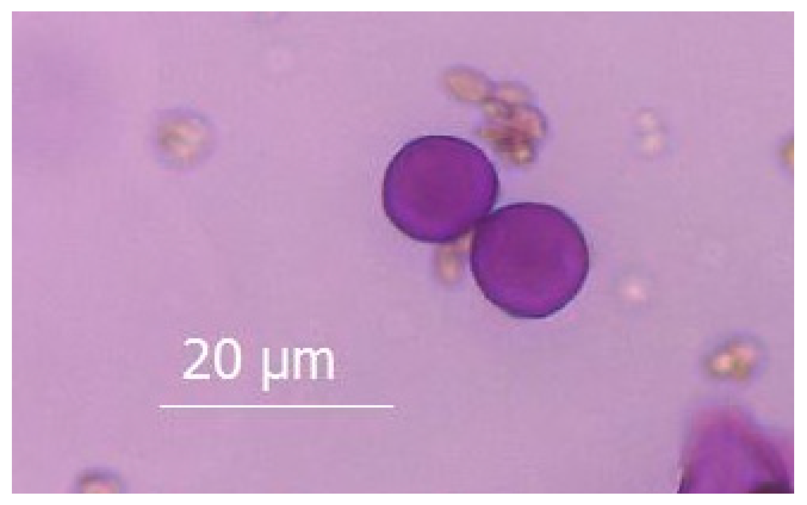
2.2. Pollen Study and Meteorological Variables

Aerobiological sampling was carried out from 1999 to 2022 using a Lanzoni VPPS-2000 Hirst type sampler [30], which was placed approximately 15 m above the ground. For the preparation and counting of pollen samples, we followed the protocol set out in the “Spanish Aerobiology Network (REA): Management and Quality Manual” [15]. The results are expressed in pollen grains per cubic metre of air, and the Seasonal Pollen Integral (SPIn), which is the sum of the daily average airborne pollen concentrations recorded during the main pollen season [31].
The percentage method was used to calculate the Parietaria main pollen season (MPS). This method considers the period during which 95% of the total accumulated pollen count is recorded. The MPS starts when the pollen count reaches 2.5% of the annual total, and ends on the day when 97.5% of the annual total is reached [32]. The selected parameters for the MPS were start (days), length (days), end (days), total pollen sum (pollen grains), pollen peak (pollen grains·m−3), pollen peak day (days), pre-peak length (days), pre-peak pollen sum (pollen grains), post-peak length (days), and post-peak pollen sum (pollen grains).
On the other hand, meteorological data series were selected from the station of the Meteorological Observation and Prediction Unit of Galicia (MeteoGalicia) located in Ourense at 300 m from the pollen trap. We considered rainfall (mm); relative humidity (%); hours of sunshine (h); and minimum, maximum, and average temperature (°C).
For machine learning model implementation, the following input variables were used: (i) the day of the year (1 to 365/366), (ii) rainfall, (iii) relative humidity, (iv–vi) minimum, maximum, and average temperatures, and (vii) hours of sunshine together with (viii) pollen concentration on the current day. Pollen concentrations one, two, and three days ahead were used as output variables.

2.3. Machine Learning Model Development

2.3.1. Procedure Carried Out

Figure 3 shows the process carried out for the development of the different models implemented in this research. The development begins with the need to create the database that will be used. From the meteorological and the palynological databases, a new combined database is created, to which the three variables to be predicted are added (one, two, and three days ahead). All cases in which any data are missing, for the input or output variables, are eliminated from the final database.
Subsequently, the final database with meteorological data of pollen concentration variables from 1999 to 2022 (both inclusive) was divided into three data groups: a first group called the training group (1999 to 2010), whose function was to train the different approximation models (step 1); a second group called the validation group (2011 to 2017), whose purpose was to locate the best model for each approximation (step 2); and finally a third group called the testing group (2018 to 2022), to check the proper generalization performance models in real use (step 3).

2.3.2. Random Forest

A random forest (RF) model is a type of supervised machine learning algorithm that is built using decision trees (DTs) [26,33] (Figure 4), in which input data are mapped to an output to find a relationship within the entire training dataset [34]. Babenko et al. (2023) [35] stated that this algorithm was created in 1995 by Ho [36].
The random forest model is a clear example of bagging in which the application of homogeneous weak learnes are used, training them in parallel and independently to combine the resulting classifiers by means a deterministic averaging process [35]. According to Vergni and Todisco (2023) [33], in regression mode, the final solution is based on the average prediction, and for classification purposes, is based on a majority vote [40]. As specified by Hossain et al. (2021) [41], an RF model has a lower probability of overfitting, produces less variance, and is almost always more accurate than DTs.
Random forest models can be used in a large number of scientific fields, such as Chemistry to identify important variables [42] or to predict molecular electronic transitions [43], in Toxicology to determine the chemical toxicity to Tetrahymena pyriformis [44], or in Food Technology to determine the significance of the structural characteristics of betaglucans [45], among others.
In this research, to obtain the best model, different combinations of hyperparameters have been created, including the number of trees, the maximum depth, and the prepruning. Each of these hyperparameters has been defined as follows: for the number of trees, the range analyzed varied from 1 to 100 using 99 linear steps; for maximal depth, the range varied between 1 and 100 using 99 linear steps; and pre-pruning was configured as true and false.
In addition, the models were implemented with the real values for each of the input and output variables. Then, different normalized models were developed using two types of normalization processes: range transformation between −1 and 1, and Z-transformation. The normalization process was first carried out in the training data. Once the normalization model was created, it was applied to the validation and test data. For these normalization models, a denormalization process was subsequently applied to compare them with the models that had not been normalized.
Taking all this into account, for the random forest algorithm, three different configurations were finally created: models without normalization (RF), models with range normalization (RFR)—denoted with subscript R, and models with Z transformation (RFZ)—denoted with subscript Z.

2.3.3. Support Vector Machine

The second group of models developed in this research corresponds to support vector machine algorithms. The SVM model is a common supervised learning approach [41], whose approach is founded on the statistical learning theory, specifically on the VC dimensional theory and the structural risk minimization principle [46]. SVM models can work with linear and non-linear data [47] and can be used for classification and other learning purposes [48]. In general, when working in regression mode, it is essential to describe a class of undefined target features before determining the learning model [49]. According to Hossain et al. (2021) [41], SVM models present some advantages such as allowing non-linear transformation by using a kernel, handling a large number of feature spaces, and the overfitting problem being lower.
These types of models are widely used in different fields such as Biology to identify species of contaminating beetles in food [47], in Medicine to determine dementia [48], or in Biochemistry to determine the toxicity of different organic compounds to Vibrio fischeri [50].
As in the previous case, in this research, different models have been carried out based on different combinations of hyperparameters. In this case, the combinations of SVM types, gamma, and C. For the first of the hyperparameters, the used types were epsilon-SVR and nu-SVR, and on the other hand, because the LibSVM library [51] was used, the recommendations proposed by Hsu et al. (2016) [52] have been followed. In this sense, the gamma was analyzed between around 3 × 10⁻⁵ and 8 in 18 steps, and C was analyzed between 0.03125 and 32,768 in 20 steps. For these last two hyperparameters, the steps were also analyzed on linear and logarithmic scales.
In the same way, as in the random forest model, the models were carried out using the real scale variables and normalized variables in range or by Z transformation. The normalization and denormalization processes were carried out identically.
With all this in mind, for the support vector machine algorithm, the following models were carried out (SVM, SVMR, and SVMZ—all of these using the linear scale, and SVML, SVMR-L, and SVMZ-L—all of these using the logarithmic scale—denoted with subscript L).

2.3.4. Artificial Neural Network

Finally, the last of the developed models are artificial neural network algorithms that have been implemented using different typologies and combinations of two different hyperparameters. Artificial neural networks (ANNs) are prediction methods inspired by how the flow of information is transmitted in the human brain [24]. The artificial neural network is made up of artificial neurons established in different layers: a input layer, one or more hidden layers (also known as intermediate layers), and a output layer [24,53]. The number of neurons in the input and output layers is defined by the input variables used and the number of output variables required [24]. According to Hossain et al. (2021) [41], an ANN model is a very suitable approximation method when the relationships are non-linear and complex, there are multiple training algorithms, and they are feasible for use in both regression and classification problems.
Artificial neural network models can be used in different scientific fields, such as in Engineering to represent complex chemistry in turbulent reactive flows [54] and in Food Technology to classify rice grains using texture analysis [55] or to classify rhubarb juice [56].
In this sense, ANN models have been developed with a single intermediate neuron layer that is made up of a certain number of neurons established by using the interval one to 2n + 1, where n is the number of input variables. The hyperparameters analyzed were the training cycles between 1 and 131,072 using 17 steps on a linear and logarithmic scale and decay (true or false). As with the previous SVM model, some models were subjected to normalization and denormalization processes, and in addition, the steps were analyzed on a linear and logarithmic scale.
With all this in mind, for the artificial neural network algorithm, the following models were carried out (ANN, ANNR, and ANNZ—all of these using the linear scale, and ANNL, ANNR-L, and ANNZ-L—all of these using the logarithmic scale).

2.4. Data Processing and Statistical Analysis

The MPS calculation was carried out using the AeRobiology package (version 2.0.1) [57] in R software (version 4.3.2), through the Rstudio interface (version 2024.12.0+467) [58]. Next, Kendall’s tau statistic was used to detect possible trends in main pollen season parameters, as well as in the meteorological data during the study period.
The good prediction performance of the different models needs to be determined using different statistical parameters, in this case, it has been decided to use the root mean square error (RMSE) [59], the mean absolute error (MAE) [59], and the correlation coefficient (r) [60].

2.5. Computer Resources and Software Used for Modelling Parietaria Pollen

The computational equipment used was two AMD Ryzen 9 7950X 16-core processors with 128 GB of RAM. Both were equipped with Windows 11 Pro.
The database used in this research was assembled using Microsoft Excel 2013 and Excel from Microsoft 365 (both from Microsoft, Redmond, WA, USA).
The machine learning models (RF, SVM, and ANN) were developed using educational and free versions of RapidMiner Studio (v. 10.2.000 from RapidMiner GmbH, now in Troy, MI, USA).
The figures were made with PowerPoint from Microsoft 365 (Microsoft, Redmond, WA, USA) and the scatter plots were made with SigmaPlot 13.0 (from Systat Software Inc. now in Palo Alto, CA, USA).

3. Results

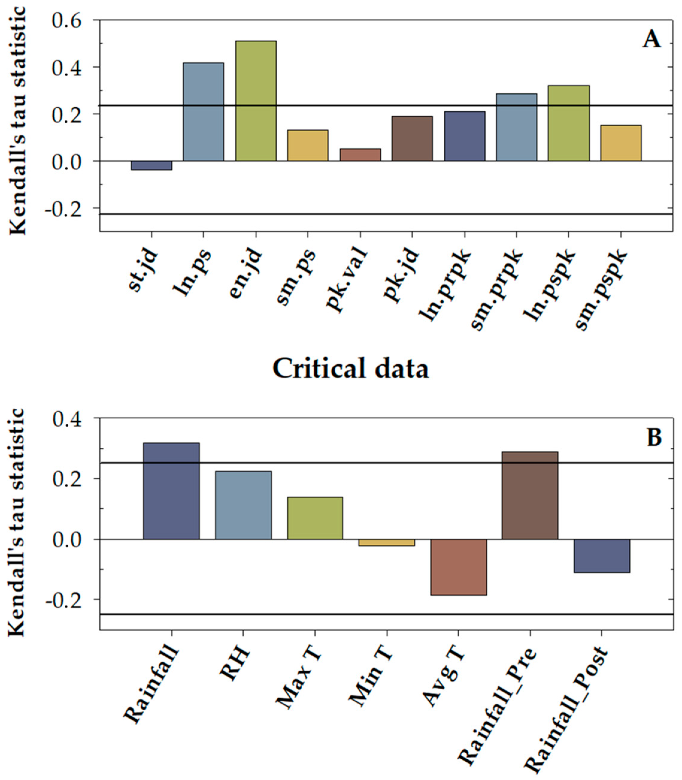
3.1. Parietaria Main Pollen Season Trends and Meteorological Trends

Over the study years, the Parietaria MPS average started on 12 March and the end date was on 31 October. The standard deviation was very similar between the start and end: 26.6% and 26.4%, respectively. The year that registered the earliest start date was 1999 on 23 January, and on the contrary the most delayed end date was on 17 December in 2015. The Parietaria MPS had an average duration of 234 days for the study period. The year with the longest duration was in 2022 with 292 days, and the shortest duration took place in 2005 (Table 1).
We observe more fluctuations in the annual pollen integral; the year with the highest annual pollen was 2016 with 3555 pollen·day/m3, and the year with the lowest pollen concentration was 2001 with 196 pollen·day/m3. If we analyze the pollen peak, we observe that the maximum value coincides with the year of the maximum annual pollen integral, in 2016, and shows a concentration of 124 pollen grains·m−3 on 20 June. The minimum value was 11 pollen grains·m−3 on July 29th in the same year that registered the minimum annual pollen integral, in 2001 (Table 1).
An increasing and significant (p < 0.05) trend was observed for the end and the length of the Parietaria MPS. An increasing and significant (p < 0.05) trend was observed as well for the pre-peak pollen sum and for the post-peak length (Figure 5).
On the other hand, only precipitation showed a significant increase (p < 0.05) during the period included in the MPS of Parietaria. Analyzing this increase in a more detailed way, it is observed that the increase in precipitation was significant only during the pre-peak period (Figure 5).

3.2. Prediction One Day Ahead

The first models were developed to predict the amount of pollen one day ahead. Table 2 shows the best models for each approach based on the smallest error committed in the validation phase.
The three random forest model configurations carried out (RF, RFR, and RFZ) presented root mean square errors like each other in the validation phase (between 6.25 and 6.26 pollen grains·m−3). According to the lowest RMSE for the validation phase, the not normalized model was the worst model, with an RMSE value of 6.25 pollen grains·m−3 offering the best adjustments for the validation phase. This model presents a correlation coefficient of 0.878 for the validation phase and an absolute error of 3.23 pollen grains·m−3. The adjustments obtained by the RF model in the training phase are notably better, reaching an RMSE value of only 2.15 pollen grains·m−3.
The following model in terms of good behaviour, according to the RMSE value in the validation phase, is the SVMR-L model. This model was the best obtained among the six types of support vector machine models carried out that obtained RMSE values between 6.12 and 6.26 pollen grains·m−3. This model presents less favourable results for the training phase than those presented by the previous RF model.
Finally, the best model considering the RMSE values in the validation phase corresponds to the ANNR-L model, which was chosen among all the ANN models that presented values between 5.92 and 6.07 pollen grains·m−3. This best ANN model is characterized by having similar behaviour values between the training and validation phases.
The three best models selected (RF, SVMR-L, and ANNR-L model), one for each approximation, present acceptable correlation coefficient values between 0.873 and 0.919 for the training and validation phases together. The results of these models in the testing phase can be seen in Table 2, where it can be seen that these models follow a similar RMSE value order to in the validation phase. This is because the random forest model presents the worst adjustments for the testing phase, with an RMSE value of 5.84 pollen grains·m−3, followed by the support vector machine model, with a value of 5.72 pollen grains·m−3, and ending with the best model in the testing phase (ANNR-L), with a value of 5.55 pollen grains·m−3. For this last model, the correlation value is 0.859, with an absolute error of 2.97. These error values, together with the high correlation coefficient, seem to indicate that this model would be able to generalize adequately for a real employment phase, which would allow predicting with the Parietaria pollen concentration in the atmosphere with the margin of one day.
Figure 6 (top) shows the temporal representation of the concentration of Parietaria pollen in the atmosphere: the real values and those predicted one day ahead (using the ANNR-L model).
As can be seen in the Figure, the prediction of the ANNR-L model can draw the time series of real concentration values one day ahead. It can be seen that, in general, the predicted value (black line) follows the trend over the grey area that represents the actual values of pollen concentration. Despite this good general fit, it is possible to observe how some peaks are underestimated in the time series. This happens especially with peaks whose value exceeds 40 pollen grains·m−3. The most notable case, at first glance, may be the highest peak area located on the left of Figure 6 (top). In this area, a group of points around the maximum (11 points) were incorrectly predicted, obtaining an absolute error of around 17.86 pollen grains·m−3, with the maximum and minimum values in this area being between 15 and 91 pollen grains·m−3.
Given the results presented in Table 2 and the model behaviour in the testing phase shown in Figure 6 (top), it can be said that, in general, the neural network model (ANNR-L) can predict the concentration of Parietaria pollen in the atmosphere with an acceptable margin of error.

3.3. Prediction Two Days Ahead

The second group of models developed were carried out to predict the pollen concentrations two days ahead. It can be seen from Table 2 that the best models for each approach are based on the smallest error obtained in the validation phase.
The three random forest model configurations carried out (RF, RFR, and RFZ) presented similar root mean square errors between 7.57 and 7.61 pollen grains·m−3. In this case, as the models predict the pollen concentration one day ahead, the model that presents the worst adjustments in terms of RMSE in the validation phase is the random forest model (in this case, a normalized random forest model (RFR)). For this model, it can be seen in Table 2 that the errors in terms of RMSE (7.57 pollen grains·m−3) and MAE (3.81 pollen grains·m−3) increase in comparison with the previous RF model (6.25 and 3.23 pollen grains·m−3), which denotes a decrease in the correlation coefficient (0.878 to 0.814 pollen grains·m−3). Similarly, the worsening of the statistics for the training phase can be observed. This behaviour occurs as expected when the prediction time window increases from one to two days ahead.
The next model in performance considering the RMSE value in the validation phase is the logarithmic SVM model that presented a close value (7.51 pollen grains·m−3) to the RFR model. This model, as with the previous RFR model, worsens its metrics compared to the model developed to predict the pollen concentration one day ahead (SVMR-L model). In this case, it can also be observed how the model improves its adjustments in the training phase in comparison to the validation phase.
The best model developed to predict Parietaria pollen concentration was the ANN model. This model was the best among the six types of ANNs developed that presented an RMSE value between 7.34 and 7.42 pollen grains·m−3 for the validation phase. In this case, the ANN model presents an RMSE value of 7.34 pollen grains·m−3 for the validation phase, with a high correlation coefficient of 0.825. Likewise, the model’s performance in the training phase is similar, with a correlation coefficient value of 0.795.
The proper behaviour of the three selected models in the validation phase can also be observed in the testing phase, in which the three models improve their statistics in terms of root mean square error and mean absolute error. This improvement does not occur for the correlation coefficient parameter, which drops from values between 0.814 and 0.825 to values between 0.754 and 0.781.
Finally, considering the lowest RMSE in the validation phase, it can be said that the best model is the not normalized and linear scale artificial neural network model. The good performance of this model (ANN) in the testing phase can be seen in Figure 6 (centre), which shows the temporal representation of the Parietaria pollen concentration in the atmosphere: the real values and the predicted ones two days ahead. As can be seen in this time series, the peak prediction is less effective than in the case of one day ahead, because the time window increases and therefore the predictions become increasingly worse, and the representation of the peaks suffers a gradual deterioration. Despite this, in general, there is a pattern of monitoring the real concentration of pollen in the atmosphere.

3.4. Prediction Three Days Ahead

Finally, the last group of selected models corresponds to the machine learning models intended to predict the pollen concentration three days ahead. As can be seen in Table 2, these models suffer a significant deterioration in their prediction capacity, which is greatly decreased, especially in the validation phase. In this case, the prediction power of the models follows a slightly different order than in the models selected to predict the pollen concentration one or two days ahead.
The model that presents the worst results for the validation phase are, in this case, the support vector machine models with the linear and the logarithmic scales. Both models offer an RMSE value of 8.43 pollen grains·m−3 for the validation phase, which places this value almost one point above the error committed in the best SVM models (SVM and SVML) to predict pollen two days ahead (7.51 pollen grains·m−3), and almost two and a half points above the model SVMR-L intended to predict pollen one day ahead (6.12 pollen grains·m−3).
The model with the second best result is the random forest model, which offers, for the validation phase, a very similar result (8.39 pollen grains·m−3) to the two SVM models, but presents the same behaviour observed as in the support vector machine models, that is, it suffers a significant increase in its error in the validation phase (8.39 vs. 7.57 pollen grains·m−3 two days ahead and 6.25 pollen grains·m−3 one day ahead), having less remarkable behaviour for the training and testing phases.
Finally, the model that presents the best adjustments, considering the lowest RMSE value in the validation phase is, once again, the artificial neural network model, which presents an RMSE value of 8.10 pollen grains·m−3 for this phase. This model offers outstanding adjustments for the testing phase (7.32 pollen grains·m−3) compared to the other selected models (7.59 and 7.66 pollen grains·m−3), and close to those obtained using the random forest and support vector machine models for the prediction two days ahead (7.17 and 7.12 pollen grains·m−3, respectively).
Considering the lowest RMSE in the validation phase, it can be said that the best model is the not normalized and linear scale artificial neural network model (ANN). The performance in the testing phase can be seen in Figure 6 (bottom), where it can be observed that there is a loss of prediction power, especially focused on the peaks on the right side of the graph. This can be observed especially in the low prediction power located in the largest peak on the right.

4. Discussion

From an environmental perspective, monitoring pollen diversity enhances the assessment of plant biodiversity by examining plant phenology. This approach enables the identification of the presence or absence of species, the composition of plant communities, and the detection of physiological changes and variations (SDG 3: Good Health and Wellbeing; SDG 11: Sustainable Cities and Communities; and SDG 15: Life on Land) [1]. Moreover, it advances the understanding of how plant communities are impacted by atmospheric warming, phenological shifts, land use changes, and biodiversity loss driven by global climate change [1,61,62]. From the people perspective, our research provides crucial information for advancing this field of sustainability. The aerobiological monitoring and prediction models developed in this study expand on the understanding of critical health issues in our region. All the information generated enhances the understanding of allergenic pollen diversity in urban areas and its relationship with various public health aspects, including the potential occurrence of cross-reactions, air pollution, adherence, rural–urban gradients, as well as genetic and socio-economic factors. The data obtained from monitoring and modelling are also utilized in the management of urban green spaces, improving recommendations to reduce exposure to allergenic pollen types and developing more effective action plans to mitigate allergy risks [1], and all these results are aligned with the Sustainable Development Goals SDG 3: Good Health and Wellbeing, and SDG 11: Sustainable Cities and Communities [63,64,65,66,67].
Finally, regarding climate sustainability aspects, numerous studies have explored the processes that correlate meteorological variables with airborne pollen. Some works focus on correlations between meteorological variables and pollen over time scales ranging from days to years [20,68]. Other studies report that variables such as temperature, sunshine hours, solar radiation, and wind speed are positively correlated, whereas precipitation and relative humidity are negatively correlated with pollen concentrations [20,69,70]. All this information is incorporated into our models as a predictor, improving their quality and providing insights to anticipate and manage the effects of climate change on human health and allergenic species in urban environments (green spaces in cities), such as in our study area (SDG 11: Sustainable Cities and Communities; SDG 13: Climate Action).
In recent decades, the field of Aerobiology has focused on researching the behaviour of airborne pollen and aeroallergens [71,72]. This has provided improved information on the role of these particles in biological air pollution [8]. Respiratory allergies represent a significant public health problem, with a notable increase in prevalence over recent decades. In Europe, it is estimated that up to 40% of the population is affected by some type of pollen allergy [8]. This percentage has demonstrated an upward trend over the past three decades, being higher in children [73]. Pollen monitoring is currently regarded as an effective tool for identifying local pollen types that are capable of inducing respiratory allergies [74]. Furthermore, the potential medical and environmental effects of these particles have led to the development of forecasting airborne pollen concentration models, such as machine learning models, which are of great importance in this field due to their applicability in the prevention, diagnosis, and treatment of allergic diseases [75].
Parietaria pollen is one of the most prevalent allergens in Europe, and is a significant outdoor allergen in most Mediterranean countries [76]. Given that the genus has a prolonged pollen season, up to 80% of patients with pollinosis in Mediterranean regions are sensitized against Parietaria allergens, with approximately 52% of these patients suffering rhinitis and asthma [76].
The most prevalent species in southern Europe is Parietaria judaica L. Due to its high pollen grain production per plant [10], prolonged flowering period [77], and abundant synthesis of allergens in the cytoplasm and cell walls [78], it is responsible for severe cases of sensitization in spring, as previously mentioned.
In this study, we analyzed the trends of the main parameters of the main pollen season of Parietaria, as well as the meteorological variables during the study period using Kendall’s tau statistic. The length and end date of the MPS demonstrated an increasing trend during the study period. The pollen content in the pre-peak period and length in the post-peak period showed an increasing trend as well. The meteorological variable with a significant trend, which was also an increasing one, was precipitation, particularly precipitation in the pre-peak period. These findings suggest that the observed increase in pollen content and rainfall during the pre-peak period may contribute to delaying the pollen season, resulting in a prolonged period of pollen detection after the peak. These results agree with the reports of different authors who explain how the highest amount of rainfall and the highest number of rainy days are ideal for the development of these herbaceous plants, which shows that rainfall has a great influence on the flowering and pollination of these plants [79,80]. In addition, the current context of the climate change situation that we are experiencing can induce an increase in air temperature and unstable rainfall, which could cause the earlier, longer, and more intense flowering of Parietaria [81,82]. These changes in the pollen concentrations of Urticaceae have already been pointed out in Thessaloniki in the period 1987–2005 [83].
The length of the Parietaria pollen season depends on meteorological factors. For example, in southern Italy, the pollen season can persist from February to December, causing symptoms throughout the year [84]. As D’Amato et al. (1992) [84] report, in other areas, such as southern France or the Mediterranean coastal region of Spain, pollination occurs from April to September [85,86]. Different authors pointed out that the influence of meteorological variables on the pre- and post-peak parameters of the pollen season for several taxa have also been studied [73]. In this work, for the Parietaria pollen type, it was found that the pollen content during the pre-peak period in the city of Malaga was negatively correlated with precipitation [73]. This reinforces the previous explanation that precipitation at the beginning of the pollen season exerts an atmospheric washing effect, resulting in the recording of the pollen content at the end of the pollen season, between July, August, and September in Ourense, when temperatures are high and the climate is drier, promoting the atmospheric dispersion of pollen grains. These results indicate an increase in the period of exposure to this pollen type, specifically in the post-peak period. However, in the present work, a significant increasing trend of precipitation in the pre-peak period is shown, and this behaviour has been highlighted by other authors for the Artemisia pollen type, who point out the same trend regarding precipitation in the pre-peak period, concluding that previous rainfall favours the pollination process [87]. Regarding Parietaria, some authors pointed out that a greater amount of rainfall and greater number of rainy days are ideal for the development of these herbaceous plants, with an increase in the production of flowers and pollen [79], and so wetter years coincide with higher concentrations of Urticaceae pollen [88]. As for the correlation analysis, a study carried out in Córdoba obtained positive correlation coefficients with rainfall [89], like in the present work.
In the literature, simple models have been used to predict pollen. An example is the multiple regression model used by Howard and Levetin (2014) [90] to determine Ambrosia pollen one day ahead. Their final model included different variables: dichotomous precipitation, minimum temperature, dew point, and phenology variable, to obtain a correlation coefficient between the observed and predicted values of 0.715 [90]. Despite the great difference between the models developed in this research and those used by these authors, the models developed here present higher correlation coefficient values to predict pollen concentration one day ahead (between 0.845 and 0.859 for the testing phase) than those obtained by Howard and Levetin (2014) [90].
Regarding machine learning models, the work carried out here can be compared with other similar works developed in the literature. The prediction of Ambrosia pollen can also be carried out by applying machine learning models. In this case the authors used environmental, and data provided by next-generation radar (NEXRAD) to predict daily pollen concentration (Tulsa, OK, USA) [91]. Zewdie et al. (2019) [91] developed prediction models based on random forest, support vector machine, and artificial neural network algorithms, with correlation coefficient values for the test phase between 0.46 and 0.61. Therefore, the results of this research present better performance parameters than the models developed by these authors [91] (considering that the pollen is different, the input variables are different, and the location is different). On the other hand, in the literature, it is possible to locate research articles to study the concentration of Olea pollen in different points of the Autonomous Community of Madrid (Spain) [92]. Cordero et al. (2021) [92] combined two-step generalized additive models with an artificial neural network and a light gradient boosting machine (LightGBM). Pollen concentration models reported determination coefficient values of around 0.6 for external validation [92]. Recently, the use of machine learning models, including random forests, support vector machines, and multilayer perceptrons, among others, to determine the days on which birch pollen concentrations exceeded predetermined levels, has been reported [93].
In 2019, a study was carried out by our research group to determine the amount of Parietaria pollen in the city of Vigo [77], which is approximately 100 km from the area studied in the present work. In that study, models were developed with artificial neural networks using thirteen input variables (using data from 1999 to 2013 in the training phase and 2014–2015 in the validation phase). Later, based on the best models developed in the validation phase, these variables were reduced to five: Parietaria pollen concentration, day, and maximum, minimum, and mean temperature [77]. These five selected variables became part of developing new models that included a testing phase for the years 2016 and 2017. These new models obtained RMSE values for the testing phase between 13.22 and 17.57 pollen grains·m−3. It seems clear that the models selected here (with RMSE values for the testing phase between 5.55 and 7.66 pollen grains·m−3) improved the models presented by Valencia et al. (2019) [77]. This notable improvement may be due to several factors, one of them could be the amplitude of pollen recorded in Vigo city used to train the models, (between 0 and 225 pollen grains·m−3, instead of the 0 to 117 pollen grains·m−3 for Ourense city). However, the values remain nearest for the testing phases, with Vigo being between 0 and 142 pollen grains·m−3 and Ourense between 0 and 91 pollen grains·m−3. Despite this notable difference, the proportion obtained in these models is still lower than that obtained in the previous models for the city of Vigo. To the best of the authors’ knowledge, this improvement is probably due to the increase in the number of years included in the database, going from 19 years to 24, and in the number of years used in the validation phase (from 2 to 7). This increase in the number of years in the validation phase has probably allowed for the selection of the most optimal models, instead of less trained models with only two years. On the other hand, it is also necessary to highlight that, since these are different locations (although located 100 kilometres apart), other biogeographic parameters not considered within these models may play a relevant role.
On the other hand, a similar study was carried out by Voukantsis et al. (2010) [94] in which prediction models were developed for one to seven days ahead, for the average daily concentrations of pollen in the air for different taxa: Urticaceae, Oleaceae, and Poaceae. The models developed to be applied in Thessaloniki (Greece) were multilayer perceptron, regression trees, and support vector regression models. Voukantsis et al. (2010) [94] concluded that these models generally perform better than traditional models based on multiple linear regression, and perform better as a combined model than as an individual model, offering index of agreement values between 0.85 and 0.93. These agreement indices decrease with the time window, in the same way as what occurs in the present research. In the models developed by Voukantsis et al. (2010) [94], it can be seen how the correlation coefficient for the individual models varies between 0.89 (one day ahead) and 0.52 (seven days ahead), while for the combination model, the variation was between 0.89 (one day ahead) and 0.72 (seven days ahead). These models presented good results; however, it is necessary to take into account that the number of variables used to determine pollen concentrations is much higher than those used in this research, so for example, for the Urticaceae models, it is necessary to increase the number of input variables up to 80 to obtain adequate predictions of pollen at 7 days [94].
In a similar study using recurrent neural networks carried out by Čorić et al. (2023) [95], different models that would be capable of predicting the daily concentrations of three types of pollen: ragweed (Ambrosia), grass (Poaceae), and birch (Betula) one and two days in advance were developed. The authors used meteorological data and pollen concentrations from between 2000 and 2021 for the city of Novi Sad. The model proposed by Čorić et al. (2023) [95] showed superior performance compared to traditional approaches, although it was observed that the prediction at maximum concentrations must be improved, since the proposed model is not capable of adequately simulating severe and extreme degrees of pollen concentration. In addition, the research also confirmed that the accuracy of the prediction decreases with the time window, a fact that can also be contrasted with the present research. The researchers conclude that recurrent neural networks can be used to predict pollen in the air.
In view of the comparisons made with the previous research articles, it can be concluded that neural network technology, whether of one category or another, can be used to predict the concentration of pollen in the air. However, it can be said that this type of approach is not only limited to the projection of pollen concentration in the air, but can also be used with good results for the discrimination of allergenic pollen. This is the case in the study carried out by Polling et al. (2021) [96] that used convolutional neural networks to increase accuracy in the control of allergenic pollen and differentiate the genera Urtica and Parietaria.
For all these reasons and in view of the results presented in this research, the authors suggest that it could possibly be a good idea to continue researching these types of models to make increasingly accurate predictions. Therefore, the authors suggest that these models could be improved by considering the following tips:
  • Study the possibility of increasing the number of input variables, not only by using variables different from those used in the present research, but also variables that include a time scale and backwards, as could have been seen in the paper carried out by Voukantsis et al. (2010) [94];
  • The authors understand that increasing the number of years in the database would be a positive fact, but it would be interesting to study the variation in the number years in the training, validation, and consultation groups to see how this modification could alter the results obtained;
  • Likewise, it would also be advisable to study a variation in the hyperparameters analyzed in this research, not only by increasing their ranges, but also by analyzing a different step series and even incorporating new hyperparameters;
  • Another interesting point to consider when improving prediction models would be to explore techniques such as the stacking or blending models. This procedure could allow for the taking advantage of the strengths of each base model when creating a combined model, allowing for improved prediction performance;
  • Finally, it would be interesting to develop a pollen neural network aimed at predicting the pollen concentration, not at a specific point, but rather in an extensive region, to see how geographic location and altitude could modify the performance of the developed models.

5. Conclusions

In the current context of climate change, which leads to an increase in temperatures and an irregular distribution of rainfall, these could be factors that cause the longer and more intense flowering of Parietaria, which indicates that it is a species with great phenotypic plasticity, that is, it adapts very well to drastic changes in the climate. The present study shows that the increase in pollen content and rainfall during the pre-peak period may contribute to delaying the pollen season, resulting in a prolonged period of pollen detection after the peak. With these results, we can contribute to the development of several Sustainable Development Goals (SDGs), such as SDG 3: Good Health and Wellbeing, SDG 11: Sustainable Cities and Communities, SDG 13 Climate Action, and SDG 15 Life on Land.
In the present research, prediction models have been developed based on different machine learning algorithms aimed at determining the amount of Parietaria pollen in the North-West part of Spain using data from 1999 to 2022. The developed models are random forest, support vector machine, and artificial neural network models, all of them widely used in different fields of science.
As can be seen above, the model that generally presents the best adjustments in all phases (training, validation, and testing) is the model based on artificial neural networks. In fact, for the testing phase, the ANNs present the best RMSE values (between 5.55 and 7.32 pollen grains·m−3), followed by the support vector machine (5.72 to 7.59 pollen grains·m−3), and the random forest model (between 5.84 and 7.66 pollen grains·m−3). These adjustments translate into correlations between 0.741 and 0.859 for the ANN models and 0.713 to 0.851 for the other models.
These values help us to understand that the selected models seem to work in an adequate manner in the testing phase, presenting good correlation values for predictions one and three days ahead.
For future works to improve the models, it could be beneficial to increase the number of years and the input variables, study different hyperparameter ranges and data distributions, or develop stacked/blending models based on the different approaches presented in this research.

Author Contributions

Conceptualization, G.A., M.F.-G. and F.J.R.-R.; methodology, G.A., R.A.F., D.A.D.-L. and G.G.; validation, G.A. and R.A.F.; formal analysis, G.A. and R.A.F.; investigation, G.A. and R.A.F.; data curation, R.A.F., D.A.D.-L. and G.G.; writing—original draft preparation, G.A. and R.A.F.; writing—review and editing, G.A., M.F.-G., D.A.D.-L., G.G. and F.J.R.-R.; visualization, G.A., R.A.F. and M.F.-G.; supervision, G.A., M.F.-G. and F.J.R.-R. All authors have read and agreed to the published version of the manuscript.

Funding

This research received no external funding.

Institutional Review Board Statement

Not applicable.

Informed Consent Statement

Not applicable.

Data Availability Statement

The datasets presented in this article are not readily available because the data are part of an ongoing study. Requests to access the datasets should be directed to the authors.

Acknowledgments

Gonzalo Astray thanks RapidMiner GmbH for the educational and free licence of RapidMiner Studio software (v 10.2.000).

Conflicts of Interest

The authors declare no conflicts of interest.

Abbreviations

end.jdEnd of the MPS
ln.prpkLength of the pre-peak period
ln.psLength of the pollen season
ln.pspkLength of the post-peak period
MPSMain Pollen Season
pk.jdPollen peak day
pk.valPollen peak
sm.prpkPollen integral of the pre-peak period
sm.psPollen integral
sm.pspkPollen integral of the post-peak period
SPInSeasonal Pollen Integral
st.jdOnset of the MPS
SDGsSustainable Development Goals
ANNArtificial neural network
ANNLArtificial neural network with logarithmic scale
ANNRArtificial neural network with range normalization and linear scale
ANNR-L Artificial neural network with range normalization and logarithmic scale
ANNZArtificial neural network with Z transformation and linear scale
ANNZ-L Artificial neural network with Z transformation and logarithmic scale
DTsDecision trees
RFRandom forest
RFRRandom forest with range normalization
RFZRandom forest with Z normalization
SVMSupport vector machine with linear scale
SVMLSupport vector machine with logarithmic scale
SVMRSupport vector machine with range normalization and linear scale
SVMR-L Support vector machine with range normalization and logarithmic scale
SVMZSupport vector machine with Z transformation and linear scale
SVMZ-L Support vector machine with Z transformation and logarithmic scale
MAEMean absolute error
rCorrelation coefficient
RMSERoot mean square error

References

  1. Hornick, T.; Richter, A.; Harpole, W.S.; Bastl, M.; Bohlmann, S.; Bonn, A.; Bumberger, J.; Dietrich, P.; Gemeinholzer, B.; Grote, R.; et al. An Integrative Environmental Pollen Diversity Assessment and Its Importance for the Sustainable Development Goals. Plants People Planet 2022, 4, 110–121. [Google Scholar] [CrossRef]
  2. Morton, S.; Pencheon, D.; Squires, N. Sustainable Development Goals (SDGs), and Their Implementation: A National Global Framework for Health, Development and Equity Needs a Systems Approach at Every Level. Br. Med. Bull. 2017, 124, 81–90. [Google Scholar] [CrossRef] [PubMed]
  3. Blaiss, M.S. Allergic Rhinitis: Direct and Indirect Costs. Allergy Asthma Proc. 2010, 31, 375–380. [Google Scholar] [CrossRef] [PubMed]
  4. Katelaris, C.H.; Sacks, R.; Theron, P.N. Allergic Rhinoconjunctivitis in the Australian Population: Burden of Disease and Attitudes to Intranasal Corticosteroid Treatment. Am. J. Rhinol. Allergy 2013, 27, 506–509. [Google Scholar] [CrossRef]
  5. Dwarakanath, D.; Milic, A.; Beggs, P.J.; Wraith, D.; Davies, J.M. A Global Survey Addressing Sustainability of Pollen Monitoring. World Allergy Organ. J. 2024, 17, 100997. [Google Scholar] [CrossRef]
  6. Pereira, C.; Cadahía, O.L.A. MESA REDONDA: POLINOSIS III Polinosis Por Parietaria. Alergol. Inmunol. Clin. 2003, 18, 61–85. [Google Scholar]
  7. Crimi, P.; Macrina, G.; Folli, C.; Bertoluzzo, L.; Brichetto, L.; Caviglia, I.; Fiorina, A. Correlation between Meteorological Conditions and Parietaria Pollen Concentration in Alassio, North-West Italy. Int. J. Biometeorol. 2004, 49, 13–17. [Google Scholar] [CrossRef]
  8. De Linares, C.; Alcázar, P.; Valle, A.M.; Díaz de la Guardia, C.; Galán, C. Parietaria Major Allergens vs Pollen in the Air We Breathe. Environ. Res. 2019, 176, 108514. [Google Scholar] [CrossRef]
  9. Del Trigo, M.M.; Rodríguez, M.V.J.; González, D.F.; Galán, C. Atlas Aeropalinológico de España; Secretariado de publicaciones de la Universidad de Leon: Leon, Spain, 2008; pp. 145–155. [Google Scholar]
  10. Guardia, R.; Belmonte, J. Phenology and Pollen Production of Parietaria judaica L. in Catalonia (NE Spain). Grana 2004, 43, 57–64. [Google Scholar] [CrossRef]
  11. Jato, V.; Fernández, I.I.; Aira, M.J. Atlas de Polen Alergógeno: Datos Aerobiologicos de Galicia (1993–1999). In Consellería de Medio Ambiente; Xunta de Galicia: Santiago de Compostela, Spain, 2001; ISBN 84-453-3058-6. [Google Scholar]
  12. Masullo, M.; Mariotta, S.; Torrelli, L.; Graziani, E.; Anticoli, S.; Mannino, F. Respiratory Allergy to Parietaria Pollen in 348 Subjects. Allergol. Immunopathol. 1996, 24, 3–6. [Google Scholar]
  13. Hájková, L.; Možný, M.; Bartošová, L.; Dížková, P.; Žalud, Z. A Prediction of the Beginning of the Flowering of the Common Hazel in the Czech Republic. Aerobiologia 2023, 39, 21–35. [Google Scholar] [CrossRef]
  14. Iglesias-Otero, M.A.; Astray, G.; Vara, A.; Galvez, J.F.; Mejuto, J.C.; Rodriguez-Rajo, F.J. Forecasting Olea Airborne Pollen Concentration by Means of Artificial Intelligence. Fresenius Environ. Bull. 2015, 24, 4574–4580. [Google Scholar]
  15. Galán, C.; Cariñanos, P.; Alcázar, P.; Domínguez, E. Manual de Calidad y Gestión de La Red Española de Aerobiología; Servicio de Publicaciones de la Universidad de Córdoba: Córdoba, Spain, 2007; ISBN 9788469063545. [Google Scholar]
  16. Fischer, B.; Hartwich, C. Flora Ibérica. Plantas Vasculares de La Península Ibérica e Islas Baleares. Hagers Handb. Pharm. Prax. 2012, 49, 563. [Google Scholar] [CrossRef]
  17. Li, C.; Polling, M.; Cao, L.; Gravendeel, B.; Verbeek, F.J. Analysis of Automatic Image Classification Methods for Urticaceae Pollen Classification. Neurocomputing 2023, 522, 181–193. [Google Scholar] [CrossRef]
  18. Zhong, J.; Xiao, R.; Wang, P.; Yang, X.; Lu, Z.; Zheng, J.; Jiang, H.; Rao, X.; Luo, S.; Huang, F. Identifying Influence Factors and Thresholds of the next Day’s Pollen Concentration in Different Seasons Using Interpretable Machine Learning. Sci. Total Environ. 2024, 935, 173430. [Google Scholar] [CrossRef]
  19. Bastl, M.; Bastl, K.; Karatzas, K.; Aleksic, M.; Zetter, R.; Berger, U. The Evaluation of Pollen Concentrations with Statistical and Computational Methods on Rooftop and on Ground Level in Vienna—How to Include Daily Crowd-Sourced Symptom Data. World Allergy Organ. J. 2019, 12, 100036. [Google Scholar] [CrossRef]
  20. Ritenberga, O.; Sofiev, M.; Siljamo, P.; Saarto, A.; Dahl, A.; Ekebom, A.; Sauliene, I.; Shalaboda, V.; Severova, E.; Hoebeke, L.; et al. A Statistical Model for Predicting the Inter-Annual Variability of Birch Pollen Abundance in Northern and North-Eastern Europe. Sci. Total Environ. 2018, 615, 228–239. [Google Scholar] [CrossRef] [PubMed]
  21. Khwarahm, N.R.; Dash, J.; Skjøth, C.A.; Newnham, R.M.; Adams-Groom, B.; Head, K.; Caulton, E.; Atkinson, P.M. Mapping the Birch and Grass Pollen Seasons in the UK Using Satellite Sensor Time-Series. Sci. Total Environ. 2017, 578, 586–600. [Google Scholar] [CrossRef]
  22. García-Mozo, H.; Yaezel, L.; Oteros, J.; Galán, C. Statistical Approach to the Analysis of Olive Long-Term Pollen Season Trends in Southern Spain. Sci. Total Environ. 2014, 473–474, 103–109. [Google Scholar] [CrossRef] [PubMed]
  23. Rodríguez-Rajo, F.J.; Valencia-Barrera, R.M.; Vega-Maray, A.M.; Suárez, F.J.; Fernández-González, D.; Jato, V. Prediction of Airborne Alnus Pollen Concentration by Using ARIMA Models. Ann. Agric. Environ. Med. 2006, 13, 25–32. [Google Scholar]
  24. Muzalyova, A.; Brunner, J.O.; Traidl-Hoffmann, C.; Damialis, A. Forecasting Betula and Poaceae Airborne Pollen Concentrations on a 3-Hourly Resolution in Augsburg, Germany: Toward Automatically Generated, Real-Time Predictions. Aerobiologia 2021, 37, 425–446. [Google Scholar] [CrossRef]
  25. Mills, S.A.; Maya-Manzano, J.M.; Tummon, F.; MacKenzie, A.R.; Pope, F.D. Machine Learning Methods for Low-Cost Pollen Monitoring–Model Optimisation and Interpretability. Sci. Total Environ. 2023, 903, 165853. [Google Scholar] [CrossRef] [PubMed]
  26. Lo, F.; Bitz, C.M.; Hess, J.J. Development of a Random Forest Model for Forecasting Allergenic Pollen in North America. Sci. Total Environ. 2021, 773, 145590. [Google Scholar] [CrossRef]
  27. Martínez Cortizas, A.; Pérez Alberti, A. Atlas Climático de Galicia; Xunta de Galicia: Santiago de Compostela, Spain, 1999; ISBN 8445326112. [Google Scholar]
  28. Rodríguez Guitián, M.A.; Ramil-Rego, P. Clasificaciones Climáticas Aplicadas a Galicia: Revisión Desde Una Perspectiva Biogeográfica. Recur. Rurais 2018, 1, 31–53. [Google Scholar] [CrossRef]
  29. Agencia Estatal Meteorolia. AEMet Guía Resumida Del Clima En España (1981–2010); Agencia Estatal Meteorolia: Madrid, Spain, 2012; pp. 1–110. [Google Scholar]
  30. Hirst, J.M. An Automatic Volumetric Spore Trap. Ann. Appl. Biol. 1952, 39, 257–265. [Google Scholar] [CrossRef]
  31. Galán, C.; Ariatti, A.; Bonini, M.; Clot, B.; Crouzy, B.; Dahl, A.; Fernandez-González, D.; Frenguelli, G.; Gehrig, R.; Isard, S.; et al. Recommended Terminology for Aerobiological Studies. Aerobiologia 2017, 33, 293–295. [Google Scholar] [CrossRef]
  32. Andersen, T.B. A Model to Predict the Beginning of the Pollen Season. Grana 1991, 30, 269–275. [Google Scholar] [CrossRef]
  33. Vergni, L.; Todisco, F. A Random Forest Machine Learning Approach for the Identification and Quantification of Erosive Events. Water 2023, 15, 2225. [Google Scholar] [CrossRef]
  34. Breda, L.S.; de Melo Nascimento, J.E.; Alves, V.; de Alencar Arnaut de Toledo, V.; de Lima, V.A.; Felsner, M.L. Green and Fast Prediction of Crude Protein Contents in Bee Pollen Based on Digital Images Combined with Random Forest Algorithm. Food Res. Int. 2024, 179, 113958. [Google Scholar] [CrossRef] [PubMed]
  35. Babenko, V.; Nastenko, I.; Pavlov, V.; Horodetska, O.; Dykan, I.; Tarasiuk, B.; Lazoryshinets, V. Classification of Pathologies on Medical Images Using the Algorithm of Random Forest of Optimal-Complexity Trees. Cybern. Syst. Anal. 2023, 59, 346–358. [Google Scholar] [CrossRef]
  36. Ho, T.K. Random Decision Forests. In Proceedings of the 3rd International Conference on Document Analysis and Recognition, Montreal, QC, Canada, 14–16 August 1995; Volume 1, pp. 278–282. [Google Scholar]
  37. Machado, G.; Mendoza, M.R.; Corbellini, L.G. What Variables Are Important in Predicting Bovine Viral Diarrhea Virus? A Random Forest Approach. Vet. Res. 2015, 46, 85. [Google Scholar] [CrossRef] [PubMed]
  38. Keshtegar, B.; Heddam, S.; Sebbar, A.; Zhu, S.-P.; Trung, N.-T. SVR-RSM: A Hybrid Heuristic Method for Modeling Monthly Pan Evaporation. Environ. Sci. Pollut. Res. 2019, 26, 35807–35826. [Google Scholar] [CrossRef] [PubMed]
  39. Abdolrasol, M.G.M.; Hussain, S.M.S.; Ustun, T.S.; Sarker, M.R.; Hannan, M.A.; Mohamed, R.; Ali, J.A.; Mekhilef, S.; Milad, A. Artificial Neural Networks Based Optimization Techniques: A Review. Electronics 2021, 10, 2689. [Google Scholar] [CrossRef]
  40. Breiman, L. Random Forests. Mach. Learn. 2001, 45, 5–32. [Google Scholar] [CrossRef]
  41. Hossain, M.E.; Khan, A.; Moni, M.A.; Uddin, S. Use of Electronic Health Data for Disease Prediction: A Comprehensive Literature Review. IEEE/ACM Trans. Comput. Biol. Bioinforma. 2021, 18, 745–758. [Google Scholar] [CrossRef] [PubMed]
  42. Lovatti, B.P.O.; Nascimento, M.H.C.; Neto, Á.C.; Castro, E.V.R.; Filgueiras, P.R. Use of Random Forest in the Identification of Important Variables. Microchem. J. 2019, 145, 1129–1134. [Google Scholar] [CrossRef]
  43. Kang, B.; Seok, C.; Lee, J. Prediction of Molecular Electronic Transitions Using Random Forests. J. Chem. Inf. Model. 2020, 60, 5984–5994. [Google Scholar] [CrossRef]
  44. Fang, Z.; Yu, X.; Zeng, Q. Random Forest Algorithm-Based Accurate Prediction of Chemical Toxicity to Tetrahymena Pyriformis. Toxicology 2022, 480, 153325. [Google Scholar] [CrossRef]
  45. Lam, K.-L.; Cheng, W.-Y.; Su, Y.; Li, X.; Wu, X.; Wong, K.-H.; Kwan, H.-S.; Cheung, P.C.-K. Use of Random Forest Analysis to Quantify the Importance of the Structural Characteristics of Beta-Glucans for Prebiotic Development. Food Hydrocoll. 2020, 108, 106001. [Google Scholar] [CrossRef]
  46. Zhou, X.; Li, X.; Zhang, Z.; Han, Q.; Deng, H.; Jiang, Y.; Tang, C.; Yang, L. Support Vector Machine Deep Mining of Electronic Medical Records to Predict the Prognosis of Severe Acute Myocardial Infarction. Front. Physiol. 2022, 13, 991990. [Google Scholar] [CrossRef] [PubMed]
  47. Bisgin, H.; Bera, T.; Ding, H.; Semey, H.G.; Wu, L.; Liu, Z.; Barnes, A.E.; Langley, D.A.; Pava-Ripoll, M.; Vyas, H.J.; et al. Comparing SVM and ANN Based Machine Learning Methods for Species Identification of Food Contaminating Beetles. Sci. Rep. 2018, 8, 6532. [Google Scholar] [CrossRef]
  48. Battineni, G.; Chintalapudi, N.; Amenta, F. Machine Learning in Medicine: Performance Calculation of Dementia Prediction by Support Vector Machines (SVM). Inform. Med. Unlocked 2019, 16, 100200. [Google Scholar] [CrossRef]
  49. Wang, J.; Tian, G.; Tao, Y.; Lu, C. Prediction of Chongqing’s Grain Output Based on Support Vector Machine. Front. Sustain. Food Syst. 2023, 7, 1015016. [Google Scholar] [CrossRef]
  50. Wu, F.; Zhang, X.; Fang, Z.; Yu, X. Support Vector Machine-Based Global Classification Model of the Toxicity of Organic Compounds to Vibrio Fischeri. Molecules 2023, 28, 2703. [Google Scholar] [CrossRef] [PubMed]
  51. Chang, C.-C.; Lin, C.-J. LIBSVM: A Library for Support Vector Machines. ACM Trans. Intell. Syst. Technol. 2011, 2, 27. [Google Scholar] [CrossRef]
  52. Hsu, C.-W.; Chang, C.-C.; Lin, C.-J. A Practical Guide to Support Vector Classification. Available online: https://www.csie.ntu.edu.tw/~cjlin/papers/guide/guide.pdf (accessed on 17 October 2022).
  53. Muravyev, N.V.; Luciano, G.; Ornaghi, H.L.; Svoboda, R.; Vyazovkin, S. Artificial Neural Networks for Pyrolysis, Thermal Analysis, and Thermokinetic Studies: The Status Quo. Molecules 2021, 26, 3727. [Google Scholar] [CrossRef]
  54. An, J.; Qin, F.; Zhang, J.; Ren, Z. Explore Artificial Neural Networks for Solving Complex Hydrocarbon Chemistry in Turbulent Reactive Flows. Fundam. Res. 2022, 2, 595–603. [Google Scholar] [CrossRef] [PubMed]
  55. Singh, K.R.; Chaudhury, S. Texture Analysis for Rice Grain Classification Using Wavelet Decomposition and Back Propagation Neural Network; Dawn, S., Balas, V.E., Esposito, A., Gope, S., Eds.; Springer International Publishing: Cham, Switzerland, 2020; pp. 55–65. [Google Scholar]
  56. Przybył, K.; Gawałek, J.; Koszela, K. Application of Artificial Neural Network for the Quality-Based Classification of Spray-Dried Rhubarb Juice Powders. J. Food Sci. Technol. 2023, 60, 809–819. [Google Scholar] [CrossRef] [PubMed]
  57. Rojo, J.; Picornell, A.; Oteros, J. AeRobiology: The Computational Tool for Biological Data in the Air. Methods Ecol. Evol. 2019, 10, 1371–1376. [Google Scholar] [CrossRef]
  58. RStudio Team. RStudio: Integrated Development Environment for R; RStudio Team: Boston, MA, USA, 2021. [Google Scholar]
  59. Wang, W.; Lu, Y. Analysis of the Mean Absolute Error (MAE) and the Root Mean Square Error (RMSE) in Assessing Rounding Model. IOP Conf. Ser. Mater. Sci. Eng. 2018, 324, 012049. [Google Scholar] [CrossRef]
  60. Asuero, A.G.; Sayago, A.; González, A.G. The Correlation Coefficient: An Overview. Crit. Rev. Anal. Chem. 2006, 36, 41–59. [Google Scholar] [CrossRef]
  61. Forrest, J.R.K. Plant–Pollinator Interactions and Phenological Change: What Can We Learn about Climate Impacts from Experiments and Observations? Oikos 2015, 124, 4–13. [Google Scholar] [CrossRef]
  62. Díaz, S.; Settele, J.; Brondízio, E.S.; Ngo, H.T.; Guèze, M.; Agard, J.; Arneth, A.; Balvanera, P.; Brauman, K.A.; Butchart, S.H.M.; et al. IPBES Summary for Policymakers of the Global Assessment Report on Biodiversity and Ecosystem Services; Intergovernmental Science-Policy Platform on Biodiversity and Ecosystem Services: Bonn, Germany. [CrossRef]
  63. Linneberg, A.; Dam Petersen, K.; Hahn-Pedersen, J.; Hammerby, E.; Serup-Hansen, N.; Boxall, N. Burden of Allergic Respiratory Disease: A Systematic Review. Clin. Mol. Allergy 2016, 14, 12. [Google Scholar] [CrossRef]
  64. Zuberbier, T.; Lötvall, J.; Simoens, S.; Subramanian, S.V.; Church, M.K. Economic Burden of Inadequate Management of Allergic Diseases in the European Union: A GA2LEN Review. Allergy 2014, 69, 1275–1279. [Google Scholar] [CrossRef]
  65. Eisenman, T.S.; Jariwala, S.P.; Lovasi, G.S. Urban Trees and Asthma: A Call for Epidemiological Research. Lancet Respir. Med. 2019, 7, e19–e20. [Google Scholar] [CrossRef] [PubMed]
  66. Treudler, R.; Zeynalova, S.; Kirsten, T.; Engel, C.; Loeffler, M.; Simon, J.-C. Living in the City Centre Is Associated with Type 1 Sensitization to Outdoor Allergens in Leipzig, Germany. Clin. Respir. J. 2018, 12, 2686–2688. [Google Scholar] [CrossRef]
  67. Ziska, L.H.; Makra, L.; Harry, S.K.; Bruffaerts, N.; Hendrickx, M.; Coates, F.; Saarto, A.; Thibaudon, M.; Oliver, G.; Damialis, A.; et al. Temperature-Related Changes in Airborne Allergenic Pollen Abundance and Seasonality across the Northern Hemisphere: A Retrospective Data Analysis. Lancet Planet. Heal. 2019, 3, e124–e131. [Google Scholar] [CrossRef] [PubMed]
  68. Tseng, Y.-T.; Kawashima, S.; Kobayashi, S.; Takeuchi, S.; Nakamura, K. Algorithm for Forecasting the Total Amount of Airborne Birch Pollen from Meteorological Conditions of Previous Years. Agric. For. Meteorol. 2018, 249, 35–43. [Google Scholar] [CrossRef]
  69. Bruffaerts, N.; De Smedt, T.; Delcloo, A.; Simons, K.; Hoebeke, L.; Verstraeten, C.; Van Nieuwenhuyse, A.; Packeu, A.; Hendrickx, M. Comparative Long-Term Trend Analysis of Daily Weather Conditions with Daily Pollen Concentrations in Brussels, Belgium. Int. J. Biometeorol. 2018, 62, 483–491. [Google Scholar] [CrossRef]
  70. Khwarahm, N.; Dash, J.; Atkinson, P.M.; Newnham, R.M.; Skjøth, C.A.; Adams-Groom, B.; Caulton, E.; Head, K. Exploring the Spatio-Temporal Relationship between Two Key Aeroallergens and Meteorological Variables in the United Kingdom. Int. J. Biometeorol. 2014, 58, 529–545. [Google Scholar] [CrossRef]
  71. Alcázar, P.; Galán, C.; Torres, C.; Domínguez-Vilches, E. Detection of Airborne Allergen (Pla a 1) in Relation to Platanus Pollen in Córdoba, South Spain. Ann. Agric. Environ. Med. 2015, 22, 96–101. [Google Scholar] [CrossRef] [PubMed]
  72. Plaza, M.P.; Alcázar, P.; Hernández-Ceballos, M.A.; Galán, C. Mismatch in Aeroallergens and Airborne Grass Pollen Concentrations. Atmos. Environ. 2016, 144, 361–369. [Google Scholar] [CrossRef]
  73. Ruiz-Mata, R.; Trigo, M.M.; Recio, M.; de Gálvez-Montañez, E.; Picornell, A. Comparative Aerobiological Study between Two Stations Located at Different Points in a Coastal City in Southern Spain. Aerobiologia 2023, 39, 195–212. [Google Scholar] [CrossRef]
  74. Sánchez Mesa, J.A.; Galán, C.; Hervás, C. The Use of Discriminant Analysis and Neural Networks to Forecast the Severity of the Poaceae Pollen Season in a Region with a Typical Mediterranean Climate. Int. J. Biometeorol. 2005, 49, 355–362. [Google Scholar] [CrossRef]
  75. Reyes, E.S.; de la Cruz, D.R.; Sánchez, J.S. First Fungal Spore Calendar of the Middle-West of the Iberian Peninsula. Aerobiologia 2016, 32, 529–539. [Google Scholar] [CrossRef]
  76. Mardones, P.; Ripoll, E.; Rojas, I.; González, M.C.; Montealegre, C.; Pizarro, D.; Córdova, A.; Torres, M.; Aguilera-Insunza, R.; Yepes-Nuñez, J.J.; et al. Parietaria Pollen a New Aeroallergen in the City of Valparaiso, Chile. Aeroboilogia 2013, 29, 449–454. [Google Scholar] [CrossRef]
  77. Valencia, J.A.; Astray, G.; Fernández-González, M.; Aira, M.J.; Rodríguez-Rajo, F.J. Assessment of Neural Networks and Time Series Analysis to Forecast Airborne Parietaria Pollen Presence in the Atlantic Coastal Regions. Int. J. Biometeorol. 2019, 63, 735–745. [Google Scholar] [CrossRef] [PubMed]
  78. Vega-Maray, A.M.; Fernández-González, D.; Valencia-Barrera, R.; Polo, F.; Seoane-Camba, J.A.; Suárez-Cervera, M. Lipid Transfer Proteins in Parietaria judaica L. Pollen Grains: Immunocytochemical Localization and Function. Eur. J. Cell Biol. 2004, 83, 493–497. [Google Scholar] [CrossRef] [PubMed]
  79. Thompson, K.; Grime, J.P.; Mason, G. Seed Germination in Response to Diurnal Fluctuations of Temperature. Nature 1977, 267, 147–149. [Google Scholar] [CrossRef]
  80. Jato, V.; Rodríguez-Rajo, F.J.; González-Parrado, Z.; Elvira-Rendueles, B.; Moreno-Grau, S.; Vega-Maray, A.; Fernández-González, D.; Asturias, J.A.; Suárez-Cervera, M. Detection of Airborne Par j 1 and Par j 2 Allergens in Relation to Urticaceae Pollen Counts in Different Bioclimatic Areas. Ann. Allergy Asthma Immunol. 2010, 105, 50–56. [Google Scholar] [CrossRef] [PubMed]
  81. Cheddadi, R.; Guiot, J.; Jolly, D. The Mediterranean Vegetation: What If the Atmospheric CO2 Increased? Landsc. Ecol. 2001, 16, 667–675. [Google Scholar] [CrossRef]
  82. Fotiou, C.; Damialis, A.; Krigas, N.; Halley, J.M.; Vokou, D. Parietaria judaica Flowering Phenology, Pollen Production, Viability and Atmospheric Circulation, and Expansive Ability in the Urban Environment: Impacts of Environmental Factors. Int. J. Biometeorol. 2011, 55, 35–50. [Google Scholar] [CrossRef] [PubMed]
  83. Damialis, A.; Halley, J.M.; Gioulekas, D.; Vokou, D. Long-Term Trends in Atmospheric Pollen Levels in the City of Thessaloniki, Greece. Atmos. Environ. 2007, 41, 7011–7021. [Google Scholar] [CrossRef]
  84. D’Amato, G.; Ruffilli, A.; Sacerdoti, G.; Bonini, S. Parietaria Pollinosis: A Review. Allergy 1992, 47, 443–449. [Google Scholar] [CrossRef] [PubMed]
  85. Charpin, H.; Davies, R.; Nolard, N.; Spieksma, F.; Stix, E. Concentration Urbaine Des Spores Dans Ies Pays de La Communauté Économique Européenne: Ies Urticacées. Rev. Fr. Allergol. 1977, 17, 181–187. [Google Scholar]
  86. Bousquet, J.; Hewitt, B.; Guérin, B.; Dhivert, H.; Michel, F.-B. Allergy in the Mediterranean Area II: Cross-Allergenicity among Urticaceae Pollens (Parietaria and Urtica). Clin. Exp. Allergy 1986, 16, 57–64. [Google Scholar] [CrossRef]
  87. Quevedo Coury, V. Influencia de La Precipitación En La Polinización de Artemisia: Repercusión En La Salud Pública; Universidad Autónoma de Barcelona: Barcelona, Spain, 2015. [Google Scholar]
  88. Recio, M.; Rodríguez-Rajo, F.J.; Jato, M.V.; Trigo, M.M.; Cabezudo, B. The Effect of Recent Climatic Trends on Urticaceae Pollination in Two Bioclimatically Different Areas in the Iberian Peninsula: Malaga and Vigo. Clim. Change 2009, 97, 215–228. [Google Scholar] [CrossRef]
  89. Alcázar, P.; Stach, A.; Nowak, M.; Galán, C. Comparison of Airborne Herb Pollen Types in Córdoba (Southwestern Spain) and Poznan (Western Poland). Aerobiologia 2009, 25, 55–63. [Google Scholar] [CrossRef]
  90. Howard, L.E.; Levetin, E. Ambrosia Pollen in Tulsa, Oklahoma: Aerobiology, Trends, and Forecasting Model Development. Ann. Allergy Asthma Immunol. 2014, 113, 641–646. [Google Scholar] [CrossRef] [PubMed]
  91. Zewdie, G.K.; Liu, X.; Wu, D.; Lary, D.J.; Levetin, E. Applying Machine Learning to Forecast Daily Ambrosia Pollen Using Environmental and NEXRAD Parameters. Environ. Monit. Assess. 2019, 191, 261. [Google Scholar] [CrossRef]
  92. Cordero, J.M.; Rojo, J.; Gutiérrez-Bustillo, A.M.; Narros, A.; Borge, R. Predicting the Olea Pollen Concentration with a Machine Learning Algorithm Ensemble. Int. J. Biometeorol. 2021, 65, 541–554. [Google Scholar] [CrossRef]
  93. Vovk, T.; Kryza, M.; Tomczyk, S.; Malkiewicz, M.; Lipiński, P.; Werner, M. Prediction of Airborne Allergenic Pollen Concentrations with Machine Learning. In Proceedings of the EGU General Assembly 2024, Vienna, Austria, 14–19 April 2024. [Google Scholar]
  94. Voukantsis, D.; Niska, H.; Karatzas, K.; Riga, M.; Damialis, A.; Vokou, D. Forecasting Daily Pollen Concentrations Using Data-Driven Modeling Methods in Thessaloniki, Greece. Atmos. Environ. 2010, 44, 5101–5111. [Google Scholar] [CrossRef]
  95. Čorić, R.; Matijević, D.; Marković, D. PollenNet-a Deep Learning Approach to Predicting Airborne Pollen Concentrations. Croat. Oper. Res. Rev. 2023, 14, 1–13. [Google Scholar] [CrossRef]
  96. Polling, M.; Li, C.; Cao, L.; Verbeek, F.; de Weger, L.A.; Belmonte, J.; De Linares, C.; Willemse, J.; de Boer, H.; Gravendeel, B. Neural Networks for Increased Accuracy of Allergenic Pollen Monitoring. Sci. Rep. 2021, 11, 11357. [Google Scholar] [CrossRef] [PubMed]
Figure 1. Microscopic photograph (40×) Parietaria pollen.
Sustainability 17 01528 g001
Figure 2. Location of the study area (Ourense) in Galicia and Europe.
Sustainability 17 01528 g002
Figure 3. Schematic diagram of the procedure carried out to develop the three machine learning models.
Sustainability 17 01528 g003
Figure 4. Scheme of a random forest model (inspired by Machado et al. (2015) [37]), a support vector regression model (inspired by Keshtegar et al. (2019) [38]), and an artificial neural network model (inspired by Abdolrasol et al. (2021) [39]).
Sustainability 17 01528 g004
Figure 5. Aerobiological and meteorological Mann–Kendal trends for each study region. The horizontal black bar shows the significance level. (A) Main aerobiological parameters of the MPS: onset of the MPS (st.jd; days), length pollen season (ln.ps; days), end of the MPS (end.jd; days), SPIn (sm.ps; pollen grains), pollen peak (pk.val; pollen grains·m−3), and pollen peak day (pk.jd; days); main aerobiological parameters of the pre-peak period: length (ln.prpk; days) and SPIn_pre peak (sm.prpk; pollen grains); main aerobiological parameters of the post-peak period: length (ln.pspk; days) and SPIn_post peak (sm.pspk; pollen grains). (B) Meteorological parameters studied: relative humidity (RH; %); rainfall (Rainfall; mm); maximum temperature (Max T; °C), mean temperature (Avg T, °C), and minimum temperature (Min T, °C). Precipitation trends were also calculated for the pre- (Rainfall_Pre) and post-peak periods (Rainfall_Post).
Sustainability 17 01528 g005
Figure 6. Real and predicted values for Parietaria pollen concentration during the testing years 2018 to 2022 for 1 day (top), 2 days (centre), and 3 days ahead (bottom), using the best selected models developed.
Sustainability 17 01528 g006
Table 1. Parietaria MPS characteristics over 24 study years: Start MPS (start date, day); End MPS (end date, day); Length MPS (days); SPIn (Seasonal Pollen Integral, pollen × day/m3); Pollen Peak (pollen grains·m3); and Pollen Peak Date (day). The average value (Mean.), maximum value (Max.), minimum value (Min.), standard deviation (SD), and relative standard deviation (RSD, %) were also calculated for all study years.
Start
MPS
End
MPS
Length
MPS
SPInPollen PeakPollen
Peak Date
199923-Jan13-Sep2343062114-Jun
20006-Feb8-Sep2162641317-Jul
20014-Feb15-Oct2541881129-Jul
200224-Apr28-Oct1886622714-Jun
200312-Mar1-Dec2653751912-Jun
200415-Feb25-Sep2242271414-Jun
200519-May4-Oct139320176-Jul
20065-Apr7-Nov21713843929-Jun
200720-Apr19-Oct1832406705-Jul
200810-Mar23-Oct22826261179-Jun
200917-Mar15-Oct21317796618-Jun
201023-Mar13-Oct20518707123-Jun
201122-Mar15-Nov23916925324-Jun
201210-Mar23-Nov25923546924-Jun
201316-Mar25-Oct22428117826-Jun
201416-Mar9-Nov23927267514-Jun
201520-Mar17-Dec27317885018-Jun
20161-Apr23-Nov237338012420-Jun
20172-Mar14-Nov25825819611-Jun
201819-Mar24-Nov25131049123-Jun
201921-Feb1-Nov2541606493-Jul
202010-Feb24-Oct25819636423-Jun
20212-Mar15-Nov25915835815-Jul
20221-Mar17-Dec292>20947011-Jul
Mean.12-Mar31-Oct23416705725-Jun
Max.19-May17-Dec292338012429-Jul
Min.23-Jan8-Sep139188119-Jun
SD26.6426.4333.141004.4132.2612.91
RSD (%)0.070.0714.1860.1356.840.04
Table 2. Adjustment for training, validation, and testing phases of the best models developed for each approximation. RMSE is the root mean square error in pollen·m−3, MAE is the mean absolute error in pollen·m−3, and r is the correlation coefficient.
TrainingValidationTesting
RMSEMAErRMSEMAErRMSEMAEr
One day ahead prediction
RF2.150.800.9696.253.230.8785.843.010.845
SVMR-L4.561.820.8456.123.310.8855.723.200.851
ANNR-L4.582.080.8425.923.180.8875.552.970.859
Two days ahead prediction
RFR2.581.100.9567.573.810.8147.173.590.754
SVML5.002.010.8107.513.670.8217.123.490.760
ANN5.142.290.7957.343.730.8256.793.490.781
Three days ahead prediction
RF2.911.200.9468.394.140.7637.663.830.713
SVM/SVML5.452.170.7738.434.060.7747.593.770.727
ANN5.402.470.7718.104.080.7817.323.640.741
Disclaimer/Publisher’s Note: The statements, opinions and data contained in all publications are solely those of the individual author(s) and contributor(s) and not of MDPI and/or the editor(s). MDPI and/or the editor(s) disclaim responsibility for any injury to people or property resulting from any ideas, methods, instructions or products referred to in the content.

