Spillover Effects of Financial Development and Globalisation on Environmental Quality in EAEU Countries

Abstract

One of the unexpected consequences of interregional integration is the risk of environmental degradation. The lack of barriers for goods, services, and economic resources within the area of integration association results in monetary expansion and facilitates economic growth. Indeed, the further consequence is environmental degradation in accordance with the Kuznets environmental curve hypothesis. Therefore, the dynamics of trade turnover and the GDP of the Eurasian Economic Union (EAEU) countries for 2023, the lack of the environmental empirical studies in the EAEU, and the impact of integration processes on environmental quality within the integration association are extremely relevant. The aim of this study is to identify the impact of integration spillover effects on the ecological footprint of five EAEU countries between 1992 and 2023. In order to achieve this research objective, an analysis sequence was carried out through the following steps: analyse the stationarity of the variables; check for cross-sectional dependence; evaluate the consistency of an estimator; calculate the Moran’s I index; estimate research results using the Spatial Error Model (SEM), Spatial Autoregressive Model (SAR), and Spatial Dubin Model (SDM), or eliminate the spatial models; analyse and diagnose the model; correct multicollinearity. By applying the Common Correlated Effects Mean Group (CCEMG) model (the model obtained showed a high coefficient of determination R-squared ~69%), the results are summarised: (1) Economic growth and integration processes have a positive and statistically significant impact on ecological footprints. (2) Financial development does not have a long-term statistically significant impact on environmental quality in the EAEU countries. These findings underscore the urgent need for a sustainability-oriented approach to economic integration within the EAEU. This study proposes a comprehensive roadmap for policymakers, emphasising the integration of green finance mechanisms, the adoption of sustainable trade practices, and the establishment of a regional environmental governance framework.

1. Introduction

According to the economic literature, integration processes have both positive (trade creation effect [1], market integration [2]) and negative (trade diversion effects [3], resource flow [4]) effects, exerting a multidirectional impact on welfare in developing nations. Besides the direct effects of integration determining directly the dynamics of socio-economic development, there are also indirect, so-called spillover effects, of integration. They indirectly affect the welfare of the population through knowledge spillover [5,6,7,8], technology diffusion [9,10], and labour market transformation [11,12]. A further indirect consequence of integration processes may be the deterioration of the environment and population quality of life.

The establishment of a common economic space in the integration of countries involves the reduction of trade barriers, unification of norms, standards, rules, and procedures, efficient allocation of economic resources, etc. Therefore, the absolute mobility of three economic resources, capital, technology, and labour force, multiply the benefits of interregional specialisation and cooperation development within the integration association space. Studies by Kurečić and Luša (2020) [13], Cheng, Zhang, and Xu (2023) [14], Iwegbu, Justine, and Borges Cardoso (2022) [15], and Barnes, Black, Markowitz, and Monaco (2021) [16] confirm the thesis of integration accelerating the economic growth of countries through the expansion of markets, financial development, intensification of production, and regional value chains.

The challenge is an increasing environmental cost as a trade-off for higher economic growth. In 1955, Simon Kuznets formulated the hypothesis concerned with economic growth leading to environmental degradation—the so-called environmental Kuznets curve (EKC) [17]. Considering the acceleration of integration processes and the dominance of the ‘more money–more production’ paradigm in the global economy, more and more researchers are paying attention to the relationship between these processes and the environmental condition (see Table 1).

Table 1. Summary of empirical results of some previous studies.

Research	The Impact on the Environment
The impact of integration on the environment
Xiao, Tan, Huang, Li, and Luo (2022) [18]	Regional integration has contributed to the reduction of carbon emissions through two primary mechanisms: the relocation of energy-intensive and highly polluting enterprises to other regions, and the enhancement of regional enterprises’ capacity to manage greenhouse gas emissions and improve energy efficiency.
Murshed, Ahmed, Kumpamool, Bassim, and Elheddad (2021) [19]	This study reveals that both regional trade integration and the transition to renewable energy collectively contribute to the reduction of carbon dioxide (CO2) emissions in South Asia. Furthermore, the findings corroborate the validity of the environmental Kuznets curve hypothesis. In contrast, financial development and urbanisation are identified as factors that exacerbate CO2 emissions, albeit only in the long term.
Lv, Zhu, and Du (2024) [20]	Regional integration exerts a significantly positive influence on achieving a synergistic balance between economic growth and environmental protection. Key mechanisms through which regional integration facilitates this dual objective include the mitigation of pollution transfer and the promotion of green transformation, thereby enabling a harmonious alignment of economic and environmental goals.
Qi, Liu, and Ding (2023) [21]	Regional integration has been demonstrated to effectively reduce urban pollutant emissions, with the emission reduction effects exhibiting significant heterogeneity across varying levels of pollution. Mechanism analysis further reveals that the green technology innovation effect, facilitated by regional integration, serves as a critical driver in promoting urban emission reduction.
Shah, AbdulKareem, Ishola, and Abbas (2023) [22]	Renewable energy consumption demonstrates a negative correlation with CO2 emissions, thereby contributing to environmental improvement, whereas fossil fuel energy consumption exacerbates environmental degradation. In contrast, the impact of regional trade integration on CO2 emissions was found to be statistically insignificant, indicating that its influence was not substantial enough to counteract or offset CO2 emissions.
He, Wang, Danish, and Wang (2018) [23]	Regional economic integration not only facilitates labour mobility but also enables the realisation of economies of scale. These dynamics, in turn, influence CO2 marginal abatement costs by affecting energy consumption, CO2 emissions, productivity growth, and technological progress. Empirical evidence indicates that the evolution of regional economic integration significantly contributes to an increase in CO2 marginal abatement costs at the 5% significance level.
Sheraz, Deyi, Mumtaz, and Ullah (2022) [24]	Financial development has been found to significantly exacerbate CO2 emissions, contributing to environmental degradation in Belt and Road Initiative (BRI) countries. In contrast, renewable energy consumption and globalisation play a mitigating role, effectively reducing CO2 emissions and enhancing environmental quality. Institutional quality, however, exhibits a positive correlation with CO2 emissions, suggesting that poor governance, corruption, weak bureaucratic systems, and inadequate enforcement of environmental regulations are key factors driving environmental degradation. Additionally, the study identifies a bidirectional causal relationship between CO2 emissions and financial development, renewable energy, and institutional quality. Furthermore, a unidirectional causal relationship is observed, with globalisation influencing CO2 emissions in BRI countries.
Li and Lin (2017) [25]	Regional integration exerts significant and robust positive effects on energy and CO2 emissions performance, with more than 70% of these effects attributable to the reduction of artificial barriers rather than geographical distance. While international openness also contributes positively to enhancing energy and CO2 emissions performance, it cannot serve as a substitute for regional integration. This is primarily due to China’s specialised role in energy-intensive manufacturing within the global economy.
The impact of financial development on the environment
Tinoco-Zermeño (2023) [26]	The findings confirm the presence of bidirectional causality between financial development and CO2 emissions, financial development and GDP, and primary energy consumption and CO2 emissions. Additionally, unidirectional causality is observed, running from financial development to energy consumption and from electricity generation to CO2 emissions. However, no empirical evidence was found to support a causal relationship between GDP and either energy consumption or CO2 emissions.
Lv and Li (2021) [27]	This study reveals that a country’s CO2 emissions can be influenced by the financial development of neighbouring countries. Specifically, the significantly negative spillover effect of financial development on CO2 emissions outweighs the significantly positive direct effect, resulting in a net-negative total effect. This suggests that financial development in neighbouring regions plays a crucial role in reducing CO2 emissions at a broader level.
Das, Brown, and McFarlane (2023) [28]	The relationship between per capita CO2 emissions and financial development exhibits cointegration, with the direction of causality running from financial development to CO2 emissions. The analysis reveals that positive and negative changes in financial development have asymmetric effects on CO2 emissions, both in the long and short term.
Zhao and Yang (2020) [29]	In the long term, a bidirectional causal relationship exists between regional financial development and CO2 emissions, whereas this relationship is not evident in the short term. The dynamic analysis further indicates that regional financial development exerts a significantly lagged inhibitory effect on CO2 emissions.
Shahbaz, Solarin, Mahmood, and Arouri (2013) [30]	This study confirms the existence of significant long-run relationships among CO2 emissions, financial development, energy consumption, and economic growth. Empirical evidence further demonstrates that financial development contributes to the reduction of CO2 emissions, while energy consumption and economic growth are associated with an increase in CO2 emissions.
Bayar, Diaconu, and Maxim (2020) [31]	The causality analysis did not identify a significant relationship between financial sector development and CO2 emissions. However, a bidirectional causal relationship was observed between primary energy consumption and economic growth, as well as between primary energy consumption and CO2 emissions. Furthermore, the long-term analysis indicated that both financial sector development and primary energy consumption exert a positive impact on CO2 emissions.
Xu, Huang, and An (2021) [32]	These findings indicate that financial development influences CO2 emissions through three primary channels: industrialisation, economic growth, and energy consumption. The effect of financial development on CO2 emissions transitions from negative to positive as industrialisation and energy consumption increase. Specifically, financial development exerts a positive impact on CO2 emissions when per capita income ranges between USD 1100 and USD 8100, whereas its impact is negative when per capita income falls below USD 1100 or exceeds USD 8100. Additionally, the economic growth channel serves as a Granger cause of both the energy consumption and technological progress channels, and this relationship is bidirectional.
Batool, Raza, Ali, and Abidin (2022) [33]	These results indicate that information and communication technology (ICT) and financial development contribute to environmental degradation in the long run, whereas their short-term impact on CO2 emissions is insignificant. In contrast, renewable energy consumption enhances environmental quality in both the short and long run. Additionally, economic growth is found to have a positive effect on CO2 emissions, while the squared term of economic growth reduces emissions, thereby supporting the inverted U-shaped environmental Kuznets curve hypothesis. The empirical findings from the Granger causality test reveal a unidirectional causal relationship from ICT and financial development to CO2 emissions, whereas a bidirectional relationship exists between renewable energy consumption and CO2 emissions.
Xiong, Zhang, and Mo (2023) [34]	Empirical findings consistently demonstrate that financial development has a significant positive impact on per capita CO2 emissions, though this relationship follows an inverted U-shaped pattern. These results offer new insights into the conflicting findings in the existing literature regarding the influence of financial development on carbon emissions. Furthermore, technological innovation and industrial structure serve as intermediary mechanisms through which financial development contributes to reducing per capita CO2 emissions, whereas economic scale has the opposite effect.
Anwar, Sinha, Sharif, Siddique, Irshad, Anwar, and Malik (2022) [35]	Empirical evidence indicates that urbanisation, financial development, and economic growth contribute to an increase in CO2 emissions, whereas renewable energy consumption mitigates CO2 emissions. In contrast, the impact of the agricultural sector on CO2 emissions is found to be insignificant.
Xu, Baloch, Danish, Meng, Zhang, and Mahmood (2018) [36]	Empirical findings suggest that financial development contributes to CO2 emissions and deteriorates environmental quality. Additionally, the results indicate that globalisation has an insignificant effect on environmental degradation, while electricity consumption is identified as the primary driver of increasing CO2 emissions in Saudi Arabia. Furthermore, a bidirectional causal relationship exists between globalisation and CO2 emissions in the long run, and financial development and CO2 emissions are found to Granger-cause each other.
Xiong, Zang, Feng, and Chen (2023) [37]	Empirical findings consistently demonstrate that China’s financial development has a significantly negative impact on per capita CO2 emissions, following an inverted U-shaped pattern.
Maji, Habibullah, and Saari (2017) [38]	The long-run results indicate that financial development contributes to increased CO2 emissions in the transportation and oil and gas sectors while reducing emissions in the manufacturing and construction sectors. However, the impact of financial development on CO2 emissions in the agricultural sector is not statistically significant. Additionally, the short-run elasticity results align with the long-run findings.
Ullah and Lin (2024) [39]	These findings indicate that financial structure exhibits an inverted U-shaped pattern in relation to the ecological footprint. It signifies that a pragmatic financial structure diminishes the ecological footprint. Moreover, industrialisation and urbanisation upsurge the ecological footprint while export diversification decreases.
The impact of economic growth on the environment
Szymczyk, Şahin, Bağcı, and Kaygın (2021) [40]	This analysis identifies positive relationships between CO2 emissions and key factors such as economic growth, energy consumption, and urban population. Additionally, it reveals a negative and statistically significant relationship between financial development and CO2 emissions. Although trade openness also exhibits a negative correlation with CO2 emissions, this relationship is found to be statistically insignificant.
Shahbaz, Hye, Tiwari, and Leitão (2013) [41]	The empirical results demonstrate that economic growth and energy consumption contribute to an increase in CO2 emissions, whereas financial development and trade openness mitigate them. The Vector Error Correction Model (VECM) causality analysis supports the feedback hypothesis, indicating a bidirectional causal relationship between energy consumption and CO2 emissions. Similarly, a bidirectional causal relationship is observed between economic growth and CO2 emissions. Furthermore, financial development is found to Granger-cause CO2 emissions.
Usman, Makhdum, and Kousar (2021) [42]	The results from the augmented mean group (AMG) estimation approach reveal that financial development, renewable energy, and trade openness significantly contribute to mitigating environmental degradation, while economic growth and the use of non-renewable energy are more responsible for environmental harm. Additionally, in the growth function, financial development, as well as the utilisation of both renewable and non-renewable energy, significantly promote economic growth.
Danish, Hassan, Baloch, Mahmood, and Zhang (2019) [43]	The Autoregressive Distributed Lag (ARDL) econometric approach reveals that economic growth increases the ecological footprint, thereby contributing to environmental degradation. Additionally, biocapacity also elevates the ecological footprint, further exacerbating environmental degradation. The causality analysis suggests that there is no causal relationship between economic growth and the ecological footprint.
Ahmed, Zhang, and Cary (2021) [44]	The long-run empirical results from the symmetric ARDL model indicate that economic globalisation and financial development contribute to an increase in the ecological footprint in Japan. In contrast, the findings from the asymmetric ARDL model reveal that both positive and negative changes in economic globalisation lead to a reduction in the ecological footprint. A positive change in financial development results in a more significant increase in the ecological footprint in the long run, whereas a negative change has a comparatively weaker effect. Energy consumption exacerbates environmental degradation by increasing the ecological footprint. On the other hand, population density reduces the ecological footprint, and the inverted U-shaped relationship between the ecological footprint and income supports the validity of the EKC hypothesis in Japan.
Makhdum, Usman, Kousar, Cifuentes-Faura, Radulescu, and Balsalobre-Lorente (2022) [45]	The ARDL results indicate that institutional quality and renewable energy utilisation significantly reduce the ecological footprint. Conversely, other factors such as financial expansion and natural resource exploitation are found to substantially increase ecological footprint levels in both the short and long term. Additionally, institutional quality, financial expansion, renewable energy, and natural resources significantly contribute to economic growth. The study also identifies a unidirectional causal relationship running from institutional quality and financial expansion to the ecological footprint. In contrast, bidirectional causality is observed between renewable energy, natural resources, ecological footprint, and economic growth.
Shahbaz, Dogan, Akkus, and Gursoy (2023) [46]	Financial development, economic growth, and non-renewable energy consumption negatively impact environmental quality by increasing the ecological footprint. In contrast, the effect of trade openness on the ecological footprint is found to be statistically insignificant. Furthermore, the results of the panel causality test indicate a unidirectional causal relationship from financial development to the ecological footprint, while a bidirectional causal relationship exists between economic growth and the ecological footprint.
Çakmak and Acar (2022) [47]	The findings indicate that (a) renewable energy consumption neither affects nor serves as a causal factor for the ecological footprint, and (b) economic growth influences and causally impacts the ecological footprint in the majority of oil-producing countries. Specifically, a 1% increase in economic growth is found to result in a 0.02828% increase in the ecological footprint.
Javeed, Siddique, and Javed (2023) [48]	The results of the Fully Modified Ordinary Least Squares (FM-OLS) analysis indicate that a 1% increase in economic growth, globalisation, biocapacity, and population density leads to an increase in the ecological footprint by 0.55%, 0.08%, 0.06%, and 0.03%, respectively. Conversely, renewable energy consumption enhances environmental quality by reducing the ecological footprint by 0.04%. Furthermore, the Granger causality analysis reveals a bidirectional causal relationship between the ecological footprint and globalisation, as well as between the ecological footprint and energy intensity.
Ahmad, Jiang, Majeed, Umar, Khan, and Muhammad (2020) [49]	The cointegration analysis confirms the existence of a stable long-run relationship among ecological footprint, natural resources, technological innovations, and economic growth. In the long run, natural resources and economic growth are found to exacerbate the ecological footprint, whereas technological innovations play a mitigating role by reducing environmental degradation. Additionally, the quadratic term for economic growth demonstrates a negative impact on the ecological footprint, providing empirical support for the EKC hypothesis.
Wang, Yan, and Zhao (2022) [50]	These findings further indicate that CO2 emissions significantly and positively drive the ecological footprint in the short term, whereas economic growth exerts a significant negative impact on the ecological footprint in the short term. This suggests that CO2 emissions act as a positive driver of the ecological footprint in both the short and long term, while economic growth serves as a negative predictor of the ecological footprint in both the short and long term in China. However, non-renewable energy consumption is not found to be a significant driver of the ecological footprint, either in the short or long term.
Ahmad, Jiang, Murshed, Shehzad, Akram, Cui, and Khan (2021) [51]	The overall findings indicate that financial globalisation and eco-innovation contribute to a reduction in the ecological footprint, whereas urbanisation exacerbates environmental degradation by increasing the ecological footprints. Furthermore, the relationship between economic growth and the ecological footprint follows an inverted U-shaped pattern, confirming the validity of the EKC hypothesis in the context of the G7 countries.
Usman, Alola, and Sarkodie (2020) [52]	The empirical findings indicate that a reduction in environmental degradation can be attributed to an increase in renewable energy consumption, as evidenced by its negative impact on the ecological footprint. Additionally, economic growth and biocapacity were found to exert upward pressure on the ecological footprint, whereas trade policy contributed to its reduction. A bidirectional causal relationship was identified between economic growth and the ecological footprint, as well as between economic growth and biocapacity. Conversely, a unidirectional causal relationship was established from trade policy to renewable energy consumption and from renewable energy consumption to biocapacity. Furthermore, the innovative accounting analysis revealed that renewable energy consumption and trade policy accounted for 14.79% and 8.41% of environmental changes, respectively, leading to an environmental deterioration of 0.60% and 9.88%.

Source: Authors.

Evaluation of the Literature

According to the literature review, (1) regional integration is a positive factor contributing to the reduction of pollution and CO₂ emissions through the redistribution of production, the introduction of new technologies, and increased energy efficiency [53]. However, economic barriers effect regional economic and environmental development [25]. Therefore, the following factors should be considered: The initial conditions of the regions, level of pollution, and the prevailing energy structure (in countries with the energy-intensive production). Moreover, many researchers highlight [22] the insufficient impact of integration to substantially reducing environmental damage. Indeed, increased trade and economic integration tend to be mitigated by higher fossil fuel usage and growing energy consumption.

(2) Financial development has a multidirectional environmental impact. On the one hand, financial markets and tools stimulate economic activity, and hence energy consumption [31,46]. On the other hand, financial development reduces environmental damage through technology modernisation and the transition to less carbon-intensive industries [40,42]. Furthermore, the environmental effects of financial development depend on the income level, urbanisation, and economic development stage of a region. However, in low-and middle-income countries, financial development usually increases CO₂ emissions [32]. Nevertheless, financial development can reduce the carbon footprint in developed countries with high income and active modernisation [34].

(3) According to many researchers, the correlation between economic growth and the environment is described by the environmental Kuznets curve. Though economic growth increases pollution in the initial stages, it helps to reduce environmental damage in the long term by introducing technology and improving energy efficiency [30,50].

(4) A literature review shows the absence of the papers devoted to the analysis of the EAEU countries environment.

Therefore, integration processes in the EAEU countries provide the research challenge of increasing economic growth rates caused by the elimination of trade barriers between countries, and the benefits of financial development that affect the environment and the improvement of the population’s quality of life.

Meanwhile, Footprintnetwork.org calculates the index of the ecological footprint, including for individual countries. It is possible to see the risks of a growing ecological deficit for four of the five economies in the EAEU (see Figure 1).

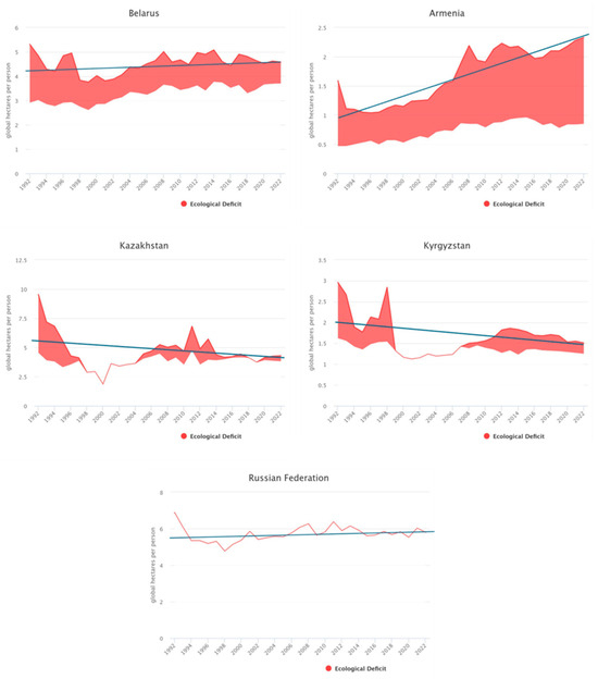
Figure 1. Environmental deficits in the EAEU countries, 1992–2022. Source: https://www.footprintnetwork.org/ (accessed on 20 November 2024).

Therefore, the dynamics of trade turnover and the GDP of the EAEU countries for 2023 (increasing up to 8% and 3%, respectively), the lack of the environmental empirical studies in the EAEU (see Table 1), and the impact of integration processes on environmental quality within the integration association are extremely relevant.

The aim of this study is to identify the impact of integration spillover effects on the ecological footprint in five EAEU countries between 1992 and 2023.

2. Methodology

The general hypothesis of this research concerns the negative impact of integration spillover effects on environmental quality in EAEU countries.

This research is based on the work of Bui Hoang Ngoca and Nguyen Huynh Mai Tramb [54] on assessing the impact of financial development and globalisation on the environmental quality of ASEAN countries to form the research model and econometric strategy.

The following indicators were used to verify the hypothesis (see Table 2).

Table 2. Main indicators profile.

Name	Abbreviations	Units	Data Sources
Gross domestic product per capita	GDP per capita	U.S. dollars, at 2015 fixed prices	World Bank
Global hectares per person	Gha per person	Points	Footprintnetwork.org
Financial development index	FDI	Percentage	International Monetary Fund
KOF globalisation index	KOF	Points	Swiss Economics Institute

Source: Authors.

The data are given in the range 1990–2023.

The boundaries of the study: five EAEU countries.

In order to achieve the research objective, the analysis sequence was carried out through the following steps.

Step 1: Analyse the stationarity of the variables.

Step 2: Check for cross-sectional dependence.

Step 3: Evaluate the consistency of an estimator.

Step 4: Calculate the Moran’s I index.

Step 5: Estimate research results using the Spatial Error Model (SEM), Spatial Autoregressive Model (SAR), and Spatial Dubin Model (SDM) or to eliminate spatial models.

Step 6: Analysis and diagnosis of the model.

Step 7: Eliminate multicollinearity.

3. Results

The spatial regression method proposed by Anselin [55] extends the classical linear regression model by considering the spatial dependence in data. Spatial dependence can occur in the dependent variable (spatial lag model, SLM) or in model errors (spatial error model, SEM).

3.1. The General Spatial Lag Model (SLM)

The General Spatial Lag Model (SLM) in its general form can be expressed as:

$$y=\rho Wy+X\beta +\epsilon$$

(1)

where

• y is a vector of a dependent variable of dimension n × 1n × 1;
• X is a matrix of independent variables of dimension n × kn × k;
• β is a vector of regression coefficients of dimension k × 1k × 1;
• W is a spatial weight matrix of dimension n × nn × n, reflecting the spatial relationships between observations;
• p is the coefficient of spatial autoregression;
• ε is the error vector, it is assumed ε∼N (0,σ2I).

In econometric analysis, the stationarity of variables is a key step in the construction of correct and reliable models. Stationarity ensures the stability of time series or panel data statistical properties. It allows ones to avoid false regressions and provide reliable conclusions. This paper analyses the stationarity of variables by several tests for panel data, including the Levin–Lin–Chu (LLC) test [56], the IPS test proposed by Im, Pesaran, and Shin (IPS) [57]. The use of multiple tests increases reliability and ensures consistency of the results. The test results are presented below (see Table 3).

Table 3. Result of panel unit root tests.

	IPS Statistic (Levels)	IPS Statistic (First Difference)	LLC Statistic (Levels)	LLC Statistic (First Difference)
Gha_per_person	−2.502845405 **	−4.964768713 **	−2.502845405 **	−4.964768713 **
FDI	−1.503180219 *	−7.618670237 **	−1.503180219 *	−7.618670237 **
GDP_per_capita	0.077397281 *	−3.735265451 **	0.077397281 *	−3.735265451 **
KOF	−3.919361581 **	−4.019112779 **	−3.919361581 **	−4.019112779 **

* Data not stationary at 5%, ** Data Stationary at 5%, Source: authors.

Based on the results of stationarity tests performed by the Levin–Lin–Chu (LLC) and Im, Pesaran, and Shin (IPS) methods, we found the following:

-

The variables Gha_per_person and KOF are stationary at significance levels of 5% and 10%. It is confirmed by negative and statistically significant values of LLC and IPS. These variables are integrated by the order of zero (I(0)) and have stable statistical properties over time;

-

The variables FDI and GDP_per_capita are non-stationary in significance levels (the values of LLC and IPS statistics do not allow rejecting the null hypothesis of the presence of a single root at significance levels of 5% and 10%). However, after taking the first differences, these variables become stationary. It indicates their integration of order one (I(1)). This result emphasises the necessity of using the first differences of these variables in the construction of econometric models or considering possible cointegration relationships to ensure the correctness and reliability of the obtained conclusions.

3.1.1. The Cross-Dependence Test

After conducting stationarity tests and determining the order of variables integration, the next step is to verify the cross-dependence in the panel data. The cross-dependence test (CD test) allows one to determine the existence of correlations between individual units in the sample not accounted for in the model. The presence of cross-dependence can cause a bias, inefficiency of estimates, and incorrect statistical conclusions.

Null hypothesis (H0):

There is no cross-dependence in the residuals:

$$H0:cov\left({\epsilon }_{it},{\epsilon }_{jt}\right)=0\forall i\ne j;\forall t$$

(2)

Alternative hypothesis (H1):

there is a cross-dependence in the residuals:

$$H1:cov\left({\epsilon }_{it},{\epsilon }_{jt}\right)\ne 0forsomei\ne j;\forall t$$

(3)

The CD test statistics are calculated as follows:

$$CD=\sqrt{{\displaystyle \frac{2T}{N\left(N-1\right)}}}{\sum }_{i=1}^{N-1}{\sum }_{j=i+1}^N{\widehat{\rho }}_{ij}$$

(4)

where:

• N is the number of individual units (cross sections);
• T is the number of time periods;
• $\rho$—assessment of the paired correlation between the residuals:

$${\widehat{\rho }}_{ij}={\displaystyle \frac{\sum _{t=1}^T{\widehat{\epsilon }}_{it}{\widehat{\epsilon }}_{jt}}{\sqrt{\sum _{t=1}^T{\widehat{\epsilon }}_{it}^2}\sqrt{\sum _{t=1}^T{\widehat{\epsilon }}_{jt}^2}}}$$

(5)

According to CD test results (see Table 4), all the studied variables have statistically significant cross-dependence between individual units in the data panel. Low p-values (significantly less than 0.05) allow one to confidently reject the null hypothesis of the absence of such a dependence. The inclusion of appropriate adjustments in the econometric model will help one to avoid bias in estimates and improve the quality of research results.

Table 4. CD-test result.

Variable Cross_Sectional_Dependence_Results	Statistic	p_Value
Gha_per_person	7.104943697	1.20372 × 10−12
FDI	11.48649614	1.54242 × 10−30
GDP_per_capita	17.22569383	1.70372 × 10−66
KOF	16.92342036	3.0235 × 10−64

Source: authors.

Once a significant cross-sectional relationship between individual units has been identified using the CD test, there is a need to correctly select a model for further analysis of the panel data. The presence of cross-sectional dependence indicates that traditional panel data models may not be sufficient to adequately describe the structure of data and a more rigorous approach to model specification is required.

3.1.2. Evaluates the Consistency of an Estimator

Particularly, it is necessary to determine whether to use a fixed effects (FE) model or a random effects (RE) model to account for individual differences in observations and to ensure unbiased and efficient parameter estimations. To address this issue, the Hausman test [58] is used to determine whether individual effects are correlated with explanatory variables. The results of the Hausman test will help to select the most appropriate model and ensure the correctness of the subsequent econometric analysis.

The Hausman test is conducted to test the hypothesis on the difference between the coefficient estimates of the FE and RE models being statistically insignificant. It indicates the random effects model is preferred. Further, we introduce the formal setting of the test, describe its hypotheses, and interpret the results obtained.

Null hypothesis (H0):

Differences in coefficient estimates between FE and RE models are statistically insignificant. It implies the individual effects are not correlated with the explanatory variables and the RE model produces consistent and efficient estimates.

$$\mathrm{H}0:cov\left({\alpha }_i,x_{it}\right)=0$$

(6)

Alternative hypothesis (H1):

Differences in coefficient estimates between FE and RE models are statistically significant. It implies the individual effects are correlated with explanatory variables and the FE model is preferred.

$$\mathrm{H}1:cov\left({\alpha }_i,x_{it}\right)\ne 0$$

(7)

Hausman test statistics is calculated as follows:

$$H={\left({\widehat{\beta }}_{RE}-{\widehat{\beta }}_{FE}\right)}^{\prime }{\left[Var\left({\widehat{\beta }}_{FE}\right)-Var\left({\widehat{\beta }}_{RE}\right)\right]}^{-1}({\widehat{\beta }}_{RE}-{\widehat{\beta }}_{FE})$$

(8)

where

• ${\widehat{\beta }}_{RE}$—vector of coefficient estimates from a model with random effects;
• ${\widehat{\beta }}_{FE}$—vector of coefficient estimates from a fixed-effects model;
• $Var\left({\widehat{\beta }}_{FE}\right),Var\left({\widehat{\beta }}_{RE}\right)$—covariance matrices of coefficient estimates for the RE and FE models, respectively.

The Hausman test statistic value is 0.2648, and the corresponding p-value is 0.9665. Since p-values are significantly higher than standard significance levels (e.g., 5% or 10%), there is no reason to reject the null hypothesis for no significant differences between the FE and RE model estimates.

It implies the individual effects are not correlated with the explanatory variables and the RE model produces consistent and efficient estimates. Therefore, the RE model is preferred for further data analysis.

3.1.3. Moran’s I Index

However, despite the correctness of the RE model in the context of individual effects, it remains necessary to consider the possible influence of spatial dependence between observations. The presence of spatial autocorrelation can disrupt the assumptions of classical econometric models on the independence of observations. It can cause biased and inefficient parameter estimates. Therefore, the next stage of the research involves testing the data for the presence of spatial autocorrelation using Moran’s I index [59]. It identifies and quantifies the degree of spatial dependence in geographic data.

Moran’s I index is used to identify and measure the degree of spatial autocorrelation in geographic data. Spatial autocorrelation is concerned with the values of a variable in one location depend on the values in neighbouring ones. The presence of spatial autocorrelation can disrupt the assumptions of classical econometric models on the independence of observations. It can cause biased and inefficient parameter estimates. Therefore, it is important to identify and consider the autocorrelation in modelling.

Moran’s I index is calculated as follows:

$$I={\displaystyle \frac{N}{W}}·{\displaystyle \frac{{\sum }_{i=1}^N{{\sum }_{j=1}^N\omega }_{ij}\left(x_i-\overline{x}\right)\left(x_i-\overline{x}\right)}{{{{\sum }_{j=1}^N(x}_i-\overline{x})}^2}}$$

(9)

where

• N—total number of observations;
• x_i—the value of the variable in location i;
• $\overline{x}$—the average value of the variable for all observations;
• $\omega$_ij—elements of the spatial weight matrix W reflecting the degree of proximity between locations i and j;
• $W=\sum _{i=1}^N\sum _{j=1}^N{\omega }_{ij}$—the sum of all the elements of the weight matrix.

Null hypothesis H0

: There is no spatial autocorrelation in the data; the values of the variable are randomly distributed in space.

$$H0:I=E\left[I\right]\approx -{\displaystyle \frac{1}{N-1}}$$

(10)

Alternative hypothesis H1:

Spatial autocorrelation is present; the values of the variable have a spatial dependence.

$$H1:I\ne E\left[I\right]$$

(11)

The results of the spatial autocorrelation testing are presented in Table 5.

Table 5. Moran’s I result.

Statistics	Gha_per_person	FDI	GDP_per_capita	KOF
Moran’s I	−0.00694	−0.00394	−0.0023344	−0.00153433
p-value	0.000	0.000	0.000	0.000

Source: Authors.

Although the results are statistically significant (low p-values), Moran’s I index values are very small in absolute value and close to zero. Although the test formally indicates a significant spatial autocorrelation, its magnitude is almost negligible. Since there is no significant spatial autocorrelation, there is no necessity to apply complex spatial models such as the Spatial Durbin Model (SDM).

Considering the identified significant cross-correlation between individual units and the absence of significant spatial autocorrelation, there is a need to adjust the model to account for the impact of common factors not captured in the original specification. Although the random effects (RE) model is recognised as the preferred model, ignoring cross-sectional dependence may cause bias and inefficient parameter estimates.

3.1.4. Common Correlated Effects Mean Group Estimator

In this regard, it is rational to apply the Common Correlated Effects Mean Group estimator (CCEMG) proposed by Pesaran (2006) [60]. This method can effectively account for the influence of uncontrolled common factors in panel data. Moreover, it may be a source of cross-sectional dependence between individual units. The use of CCEMG provides consistent and asymptotically normal estimates of the model coefficients in the presence of common factors correlated with the explanatory variables.

Consider a panel regression model:

$$y_{it}={\alpha }_i+{\beta }^{\prime }{x}_{it}+u_{it}$$

(12)

where

• $y_{it}$—the dependent variable for the individual unit i at time t.
• $x_{it}$—vector of explanatory variables of dimension $k\times 1$.
• ${\alpha }_i$—individual fixed effect.
• $\beta$—vector of the coefficients of dimension $k\times 1$.
• $u_{it}$—model error accounting for unobserved common factors.

The error is assumed $u_{it}$ to consist of unobserved common factors and random error:

$$u_{it}={\lambda }_i^{\prime }{f}_t+{\epsilon }_{it}$$

(13)

where

• $f_t$—is a vector of unobservable general dimension factors $r\times 1$.
• ${\lambda }_i^{\prime }$—vector of individual loads (factor loadings) of dimension $r\times 1$.
• ${\epsilon }_{it}$—a random error, ${\epsilon }_{it}~IID(0,{\sigma }^2)$.

A complete model considering common factors:

$$y_{it}={\alpha }_i+{\beta }^{\prime }{x}_{it}+{\lambda }_i^{\prime }{f}_t{+\epsilon }_{it}$$

(14)

However, since they are $f_t$ unobservable, it is impossible to directly include them in the model. The CCEMG method suggests using the average values of variables for all individuals as a proxy for unobserved common factors.

Enter the cross-sectional average values:

$${\overline{y}}_t={\displaystyle \frac{1}{N}}{\sum }_{i=1}^N{y}_{it}{\overline{x}}_t={\displaystyle \frac{1}{N}}{\sum }_{i=1}^N{x}_{it}$$

(15)

Using these averages, specification of the model is as follows:

$$y_{it}={\alpha }_i+{\beta }^{\prime }{x}_{it}+c^{\prime }\overline{z_t}{+\epsilon }_{it}$$

(16)

where

• $\overline{z_t}$—a vector containing the average values of the dependent and explanatory variables: $\overline{z_t}=({\overline{y}}_t,{\overline{x}\prime }_t)$’
• $c$—a vector of coefficients reflecting the influence of general factors through average values.

CCEMG final model:

$$y_{it}={\alpha }_i+{\beta }^{\prime }{x}_{it}+{\varphi }^{\prime }{\overline{x}}_t+{\psi }^{\prime }{\overline{y}}_t{+\epsilon }_{it}$$

(17)

where

• $\varphi$ and $\psi$ are the coefficients corresponding to the average values of the explanatory and dependent variables, respectively.

For the final model specification for the data, we have the following:

$$Gh{a}_{pe{r\_capita}_{it}}={\alpha }_i+{\beta }_{1}FD{I}_{it}+{\beta }_{2}GD{P}_{pe{r\_capita}_{it}}+{\beta }_{3}KO{F}_{it}+{\theta }_1{\overline{FDI}}_t+{\theta }_2\overline{GDP\_per\_capit{a}_t}+{\theta }_3{\overline{KOF}}_t{+\epsilon }_{it}$$

(18)

where

• ${\overline{FDI}}_t,\overline{GDP\_per\_capit{a}_t}$, ${\overline{KOF}}_t$are the average values of the corresponding variables at time t;
• ${\alpha }_i$—individual effect for each country;
• ${\beta }_1,{\beta }_2,{\beta }_3$—coefficients of influence of individual variables;
• ${\theta }_1,{\theta }_2,{\theta }_3$—coefficients of influence of the average values of variables (proxies for common factors).

Model statistics (see Table 6):

Table 6. Results of model estimation using CCEMG.

Variable	Coefficient Estimation	The Standard Error	t-Statistics	p-Value	Value
Constant	6.8679	0.78465	8.7529	4.339 × 10−15	***
FDI	−1.7236	1.5836	−1.0884	0.27819
GDP_per_capita	0.00051559	0.000054257	9.5027	<2.2 × 10−16	***
KOF	0.070859	0.028408	2.4944	0.01372	*
mean_FDI	−0.14440	5.1264	−0.0282	0.97757
mean_GDP_per_capita	0.00024937	0.00016427	1.5180	0.13115
mean_KOF	−0.18384	0.040502	−4.5390	1.162 × 10−5	***

* Data stationary at 5%, *** Data Stationary at any level of significance, Source: Authors.

• Total Sum of Squares: 475.42;
• Residual Sum of Squares: 147.53;
• Coefficient of determination (R-squared): 0.69857;
• Adjusted coefficient of determination (Adj. R-squared): 0.68635;
• F-model statistics: 57.1654;
• Degrees of freedom (df): 6 (numerator), 148 (denominator);
• p-value of the F-test: < 2.22 × 10⁻¹⁶.

The model explains about 69.86% of the variation in the dependent variable. It indicates a good level of its explanatory power. The constant is significant at the level of 1% and shows the basic value of the environmental indicator with zero values of independent variables. GDP_per_capita has a positive and statistically significant impact on the environmental indicator (p < 0.001). It indicates that the increase in GDP per capita is related to the increase in the environmental indicator. Indeed, KOF also has a positive and statistically significant effect on the environmental indicator (p < 0.05). It suggests a relationship between the level of globalisation and environmental performance. However, mean_KOF has a negative and statistically significant effect (p < 0.001). It may reflect the impact of globalisation trends on the environmental indicator as a whole. The remaining variables (FDI, mean_FDI, mean_GDP_per_capita) are not statistically significant. It indicates the absence of an identified influence on the dependent variable within the framework of the model.

The provided correlation matrix shows the degree of relationship between the model variables (see Table 7).

Table 7. Correlation matrix of variables.

Variables	FDI	GDP_per_capita	KOF	mean_FDI	mean_GDP_per_capita	mean_KOF
FDI	1.0000	0.8031	0.6693	0.3615	0.3358	0.3405
GDP_per_capita	0.8031	1.0000	0.5819	0.4527	0.4873	0.4522
KOF	0.6693	0.5819	1.0000	0.8116	0.7996	0.8616
mean_FDI	0.3615	0.4527	0.8116	1.0000	0.9290	0.9420
mean_GDP_per_capita	0.3358	0.4873	0.7996	0.9290	1.0000	0.9280
mean_KOF	0.3405	0.4522	0.8616	0.9420	0.9280	1.0000

Source: Authors.

Observations of the correlation matrix are as follows:

• High correlation between FDI and GDP_per_capita (0.8031): financial development and GDP per capita are closely related;
• Strong correlation between KOF and mean_KOF (0.8616): expected, since mean_KOF is the average value of KOF;
• A very high correlation between the average values of the variables:

  ○

  mean_FDI and mean_GDP_per_capita: 0.9290;

  ○

  mean_FDI and mean_KOF: 0.9420;

  ○

  mean_GDP_per_capita and mean_KOF: 0.9280.

3.1.5. Variance Inflation Factor (VIF) Analysis

VIF measures the degree of multicollinearity between explanatory variables. VIF values above 5 or 10 indicate a serious multicollinearity problem (see Table 8).

Table 8. VIF Analysis.

Variable	VIF
FDI	8.876
GDP_per_capita	4.598
KOF	14.137
mean_FDI	12.153
mean_GDP_per_capita	10.011
mean_KOF	21.334

Source: Authors.

Variables with high multicollinearity (VIF > 10):

• KOF: 14.137;
• mean_FDI: 12.153;
• mean_GDP_per_capita: 10.011;
• mean_KOF: 21.334.

Variables with moderate multicollinearity (VIF close to 10):

• FDI: 8.876.

Reasons for multicollinearity:

• The inclusion of the average values of the variables mean_FDI, mean_GDP_per_capita, and mean_KOF strongly correlate with the corresponding individual variables and with each other;
• Economic relationships: variables reflect related economic processes (globalisation, financial development, economic growth).
  Exclusion of the average values of variables:

  ○

  The average values cause high multicollinearity;

  ○

  Consider alternative methods of accounting for common factors; for example, models with fixed time effects.

After detecting high multicollinearity in the inclusion of the mean values of the variables in the model (under the common correlated effects method, CCE), it was decided to re-estimate the model without their inclusion. It allows us to assess the effect of exclusion of the average values on the quality of the model and eliminating the problem of multicollinearity. The results of the new model and their comparison with previous results are presented below (see Table 9).

Table 9. Final model.

Variable	Coefficient Estimation	The Standard Error	t-Statistics	p-Value	Value
FDI	−1.7236	1.7127	−1.0064	0.31624
GDP_per_capita	0.00051559	0.00005868	8.7865	1.237 × 10−14	***
KOF	0.070859	0.030723	2.3064	0.02279	*

* Data stationary at 5%, *** Data Stationary at any level of significance. Source: authors.

Model statistics:

• Total Sum of Squares: 475.42;
• Residual Sum of Squares: 147.53;
• Coefficient of determination (R-squared): 0.68969;
• Adjusted coefficient of determination (Adj. R-squared): 0.68635;
• F-model statistics: 57.1654;
• Degrees of freedom (df): 3 (numerator), 121 (denominator);
• p-value of the F-test: < 2.22 × 10⁻¹⁶.

The reassessment of the model without including the average values of the variables was successful. The problem of multicollinearity was eliminated, while the main results and interpretations were maintained. It confirms the expediency of using a fixed-time effects model to account for common factors and ensure reliable and interpretable research results.

3.1.6. Evaluation of the Econometric Strategy of the Research

During the research, SDM, SEM, and SAR models were initially considered to account for spatial dependence and countries cross-correlation. These models allow one to effectively accommodate the influence of spatial effects. Indeed, they play an important role in analyses of environmental and economic indicators.

However, the analysis of Moran’s I spatial autocorrelation index showed its absolute value is close to zero although the values were statistically significant. It indicates the existence of spatial dependence in the data. However, its influence is minimal and is not a key factor determining the results.

Therefore, the use of SDM, SEM, and SAR models, requiring explicit specification of a spatial weight matrix and assuming significant spatial effects, was found to be redundant. The CCEMG method was chosen.

(1)

It allows one to consider cross-correlation and the influence of common factors without having to specify a spatial structure.

(2)

It is more flexible in conditions with a weak expression of a spatial dependence.

(3)

It takes into account global and regional trends through the inclusion of average values of variables. This makes it especially relevant for the EAEU countries.

Therefore, the choice of CCEMG is provided by the results of the preliminary analysis. It corresponds with the characteristics of the research. All of the above provided a correct and stable assessment minimising the risks of distortion associated with excessive specification of spatial effects.

To ensure the sustainability and reliability of the results obtained, the following measures were taken: (1) Analysis of the stationarity of variables: LLC and IPS tests confirmed the reason for first difference applications for non-stationary variables such as FDI. (2) Elimination of multicollinearity: the VIF analysis revealed a high correlation between the average values of the variables and the corresponding individual indicators. It was eliminated by excluding the average values of the variables from the model. (3) Correction for cross-dependence: the CCEMG approach was used to consider common factors potentially affecting cross-dependence between countries, thereby improving the quality of the assessments and ensuring their consistency.

These measures ensured the correct interpretation of the impact of economic growth and globalisation on the ecological footprint of the EAEU countries. Moreover, it minimises the risk of statistical distortions.

4. Discussion

This study provides a comprehensive analysis of the spillover effects of financial development, economic growth, and regional integration on ecological footprints in the EAEU from 1990 to 2023, offering critical insights into their environmental impact.

The final model with fixed time effects uses the variables FDI, GDP_per_capita, and KOF. The model obtained showed a high coefficient of determination (R-squared ~69%). It means that the model explains about 69% of the variation in the dependent variable (ecological footprint) due to the included factors: economic growth, level of globalisation, and financial development. Hence, it has a high level of explanatory ability for the research involving panel data with spatial effects. It indicates a good level of explanatory power while the problem of multicollinearity was successfully eliminated and the main results of the model remained stable after adjustment. Moreover, it confirms the chosen model specification.

The results of the research are as follows:

Firstly, economic growth has a positive and statistically significant impact on ecological footprint. This finding aligns with the hypothesis proposed in this study, as well as with the EKC framework. The results are consistent with prior research conducted by Alola, Bekun, and Sarkodie (2019) [61] for 16 EU countries during the period 1997–2014, Danish, Hassan, Baloch, Mahmood, and Zhang (2019) [43] for Pakistan in the period 1971–2014, Ahmed and Zafar (2020) [62] for G7 countries between 1971 and 2014, Nathaniel, Anyanwu, and Shah (2020) [36] for the countries of the MENA region, and Ngoc and Huynh (2024) [54] for 10 ASEAN countries between 1992 and 2021. These studies collectively corroborate the observed relationship between economic growth and ecological footprints, reinforcing the validity of the findings.

Secondly, integration processes have a positive and statistically significant impact on ecological footprints. This outcome aligns with the hypothesis presented in the study, as well as with established international trade theories. According to these theories, when a government injects additional capital into its economy, it directly influences the competitiveness of its goods relative to those of neighbouring countries, primarily through exchange rate mechanisms. This, in turn, indirectly impacts the economic growth of neighbouring nations. Accelerated economic growth, driven by increased commodity turnover, can adversely affect environmental quality by escalating energy consumption, amplifying consumer demand, and fostering industrial expansion. However, the findings of this study contrast with the conclusions drawn by Xiao, Tan, Huang, Li, and Luo (2022) [18], Murshed, Ahmed, Kumpamool, Bassim, and Elheddad (2021) [19], Lv, Zhu, and Du (2024) [20], and Qi, Liu, and Ding (2023) [21]. According to these studies, the integration allows one to redistribute environmental costs between countries, and reduce environmental damage through knowledge spillover and diffusion of technologies. Therefore, this contradiction requires a detailed study of both the unique features of the EAEU and the differences in the methodology of previous research. The study can assume the following: (1) The nature of labour migration in the EAEU is associated primarily with unskilled labour migration. It causes the absence of knowledge and technology spillover (workers are employed in low-skilled sectors of the economy). (2) According to Chen and Lee’s hypothesis (2020) [63] on inequality at the level of economic development effects on the environment, new technologies increase the decarbonisation effect in EAEU developed economies (Russia, Kazakhstan) by the slower development of less-developed ones (Belarus, Armenia, and Kyrgyzstan). (3) High rates of economic growth and trade turnover in the EAEU could increase energy and fossil fuels consumption, negatively affecting the environment [22].

Hence, financial development does not have a statistically significant impact on ecological footprint in the EAEU countries over the long term. It correlates with the papers by Das, Brown, and McFarlane (2023), [28] and Bayar, Deaconu, and Maxim (2020) [31]. A possible explanation is that the EAEU countries have a low degree of financial markets connectivity. Moreover, they have been influenced by industrial structure, consumption of fossil fuels, commodity turnover, etc.

5. Conclusions and Policy Implications

5.1. Future Research Direction

Consequently, economic growth and integration processes exert a direct adverse impact on the environment within the EAEU. It agrees with the research hypothesis put forward. Meanwhile, the data obtained as a result of the research revealed several blind spots in the surveys devoted to the socio-economic development of EAEU countries:

(1)

To explain the contradictory relationship between integration and environmental degradation in the EAEU, it is necessary to consider the impact of knowledge spillover and technology diffusion in the EAEU on the quality of production (green transformation, fossil fuel energy vs. renewable energy) and, consequently, on environmental quality;

(2)

To explain the further impact of economic growth on the environment in the EAEU countries, it is necessary to consider the issue related to the growth of the population’s welfare and the increase in the level of consumption on environmental degradation;

(3)

To explain the absence of financial development impact on the environment, it is necessary to analyse the impact of financial development in the EAEU leading economies on energy consumption, CO₂ emission, economic growth, etc.

Searching for answers to the formulated research questions will be an issue for the following research.

5.2. Recommendations for the EAEU Countries

The findings of the conducted research underscore the necessity for adopting a sustainability-focused approach to economic integration within the EAEU. The practical significance of the research involves a number of policy recommendations for EAEU countries (see Table 10).

Table 10. Policy recommendations for the EAEU.

Key Actions	Justification	Example
The Economy policy framework (highest priority)
Introduce Turnover Penalties for High Emitters	Targeting the largest polluters ensures rapid emission reductions and generates revenue for green initiatives	The EU ETS has successfully reduced emissions in high-impact sectors like energy and aviation
Implement Tax Incentives and Subsidies for Green Technologies	Financial incentives accelerate the adoption of renewable energy and energy-efficient technologies	Germany’s Renewable Energy Act (EEG) spurred massive growth in solar and wind energy
Establish Green Economic Zones	These zones attract investment in sustainable industries and serve as hubs for green innovation	China’s Shenzhen SEZ became a global leader in electric vehicles and renewable energy
Develop a Low-Carbon Trade Model	Tariffs on high-emission imports protect domestic industries and encourage trading partners to adopt greener practices	The EU Carbon Border Adjustment Mechanism (CBAM) is designed to prevent carbon leakage.
The Institutional policy framework (second priority)
Create a Unified Environmental Monitoring System	Real-time data on air, water, and soil quality enables timely responses to environmental issues	South Korea’s Air Quality Monitoring Network has significantly improved pollution management
Establish Joint R&D Programs for Green Technologies	Collaboration accelerates the development and adoption of clean technologies	The Nordic Green Energy Research Initiative has made the region a leader in wind energy and sustainable urban development
Introduce Mandatory ESG Disclosure and Rankings	Transparency in environmental, social, and governance practices drives corporate accountability and attracts green investment	France’s Article 173 requires institutional investors to disclose ESG integration, boosting sustainable finance
Create an Intergovernmental Eco-Credit System	Subsidised green loans reduce the financial burden on companies transitioning to sustainable practices	India’s Green Credit Programme has driven rapid growth in renewable energy
The Social policy framework (third priority)
Launch Educational Campaigns for Eco-Awareness	Public awareness drives behavioural change and creates a culture of sustainability	Japan’s Eco-School Program has integrated environmental education into school curricula, fostering long-term eco-awareness
Provide Subsidies for Household Green Technologies	Financial incentives make green technologies accessible to households, accelerating adoption	California’s Solar Initiative (CSI) has led to over 1.5 million residential solar installations
Engage Citizens in Eco-Volunteering and Community Initiatives	Community involvement fosters a sense of ownership and responsibility for the environment	India’s Swachh Bharat Mission mobilised millions of citizens to clean public spaces, improving urban cleanliness
Promote Green Investment Education	Educating citizens about sustainable finance mobilises private capital for green projects	The Netherlands’ Green Bond Framework has funded renewable energy and public transport projects while raising public awareness

Source: Authors.

Prioritising economic, institutional, and social policy frameworks is critical to ensuring a balanced and effective implementation of sustainability policies. The economic policy framework serves as the cornerstone for sustainable development by establishing incentives for green innovation, reducing emissions, and promoting low-carbon industries. In the absence of such economic mechanisms, institutional and social efforts may face challenges related to funding, enforcement, and scalability. Concurrently, robust institutional policy frameworks are essential to ensure the effective implementation, monitoring, and enforcement of sustainability initiatives. Without strong governance structures, economic and social policies may suffer from a lack of coordination, transparency, and accountability. Furthermore, social policy frameworks play a pivotal role in ensuring that the transition to a green economy is inclusive and equitable, thereby fostering public support and facilitating behavioural change. However, without the foundational support of economic and institutional frameworks, social initiatives may struggle with insufficient funding, weak enforcement, or limited scalability. By adopting this prioritised approach, the EAEU can more effectively achieve its sustainability objectives while addressing potential challenges and navigating trade-offs inherent in the process.

5.3. Policy Implications

(1)

The Economy policy implications for the EAEU

Positive Implications:

• Stimulating Green Innovation: Tax incentives, subsidies, and penalties for high carbon emissions will encourage companies to adopt cleaner technologies and invest in renewable energy, fostering innovation in green technologies.
• Competitive Advantage: Companies that adopt low-carbon practices may gain a competitive edge in international markets, especially as global demand for sustainable products grows.
• Job Creation: The shift toward renewable energy and energy-efficient technologies can create new jobs in sectors like solar panel manufacturing, wind energy, and green construction.
• Trade Benefits: The “low-carbon trade” model and tariffs on high-emission imports can promote sustainable trade practices and protect domestic industries that comply with environmental standards.

Challenges and Trade-offs:

• Short-term Costs: Implementing strict emission norms and penalties may increase operational costs for businesses, particularly in carbon-intensive industries, potentially leading to resistance or economic strain.
• Regulatory Burden: Smaller businesses may struggle to comply with new regulations, requiring targeted support to avoid disproportionate impacts.
• Global Competitiveness: If neighbouring regions or trading partners do not adopt similar measures, businesses in the EAEU may face competitive disadvantages in global markets.

(2)

The Institutional policy implications for the EAEU

Positive Implications:

• Improved Environmental Governance: A unified monitoring system for air, water, and soil quality will enhance transparency and accountability, enabling timely responses to environmental issues.
• Technology Transfer: Joint R&D programs and technology transfer initiatives can accelerate the adoption of clean technologies, particularly in developing regions within the EAEU.
• Prevention of Environmental Dumping: Strict regulations on the relocation of polluting industries will prevent “environmental dumping” and ensure a level playing field across member states.
• ESG Integration: Mandatory ESG risk disclosure and rankings will encourage companies to adopt sustainable practices, improving their long-term resilience and reputation.

Challenges and Trade-offs:

• Coordination Complexity: Establishing cross-border systems (e.g., monitoring, R&D programs, and eco-credit systems) requires significant coordination among EAEU member states, which may face differing priorities and capacities.
• Enforcement Costs: Ensuring compliance with new regulations and monitoring systems will require substantial financial and administrative resources.
• Resistance from Industry: Companies reliant on carbon-intensive practices may lobby against stricter regulations, potentially delaying implementation.

(3)

The Social policy implications for the EAEU

Positive Implications:

• Behavioural Change: Educational campaigns, eco-awareness initiatives, and incentives for sustainable practices (e.g., solar panels, energy-efficient buildings) can drive long-term behavioural change among citizens.
• Community Engagement: Involving schools, universities, and local communities in environmental activities (e.g., eco-clubs, volunteering) will foster a culture of sustainability and collective responsibility.
• Financial Inclusion: Tax deductions and subsidies for households adopting green technologies will make sustainable practices more accessible, particularly for low- and middle-income groups.
• Public Health Benefits: Reduced pollution and improved environmental quality will lead to better public health outcomes, lowering healthcare costs and improving quality of life.

Challenges and Trade-offs:

• Initial Investment Costs: While subsidies and tax incentives can offset costs, the initial investment required for green technologies (e.g., solar panels) may still be a barrier for some households.
• Cultural Resistance: Changing deeply ingrained behaviours (e.g., reliance on plastic bags, fossil fuels) may take time and require sustained efforts in education and awareness.
• Equity Concerns: Ensuring that green policies benefit all segments of society, including marginalised groups, will require targeted measures to avoid exacerbating existing inequalities.

The proposed policies have far-reaching implications for the EAEU, with the potential to transform its economic, institutional, and social landscape. While the transition to a low-carbon economy presents challenges, the long-term benefits—such as improved environmental quality, public health, and economic resilience—outweigh the short-term costs. Successful implementation will require strong political will, cross-border cooperation, and targeted support for vulnerable groups and industries. By aligning economic incentives with environmental and social goals, the EAEU can position itself as a leader in sustainable development.

Hopefully, the data obtained and the problems addressed will activate a new wave of applied research on the impact of spillover effects of integration on living standards in the EAEU countries.

References

- Ahmad, M.; Jiang, P.; Majeed, A.; Umar, M.; Khan, Z.; Muhammad, S. The dynamic impact of natural resources, technological innovations and economic growth on ecological footprint: An advanced panel data estimation. Resour. Policy 2020, 69, 101817. [Google Scholar] [CrossRef]
- Ahmad, M.; Jiang, P.; Murshed, M.; Shehzad, K.; Akram, R.; Cui, L.; Khan, Z. Modelling the dynamic linkages between eco-innovation, urbanization, economic growth and ecological footprints for G7 countries: Does financial globalization matter? Sustain. Cities Soc. 2021, 70, 102881. [Google Scholar] [CrossRef]
- Ahmed, Z.; Zafar, M.W.; Ali, S. Danish Linking urbanization, human capital, and the ecological footprint in G7 countries: An empirical analysis. Sustain. Cities Soc. 2020, 55, 102064. [Google Scholar] [CrossRef]
- Ahmed, Z.; Zhang, B.; Cary, M. Linking economic globalization, economic growth, financial development, and ecological footprint: Evidence from symmetric and asymmetric ARDL. Ecol. Indic. 2021, 121, 107060. [Google Scholar] [CrossRef]
- Alola, A.A.; Bekun, F.V.; Sarkodie, S.A. Dynamic impact of trade policy, economic growth, fertility rate, renewable and non-renewable energy consumption on ecological footprint in Europe. Sci. Total. Environ. 2019, 685, 702–709. [Google Scholar] [CrossRef]
- Anselin, L. Spatial Econometrics: Methods and Models; Springer: Dordrecht, The Netherlands, 1988; Volume 4. [Google Scholar] [CrossRef]
- Anwar, A.; Sinha, A.; Sharif, A.; Siddique, M.; Irshad, S.; Anwar, W.; Malik, S. The nexus between urbanization, renewable energy consumption, financial development, and CO2 emissions: Evidence from selected Asian countries. Environ. Dev. Sustain. 2022, 24, 6556–6576. [Google Scholar] [CrossRef]
- Barnes, J.; Black, A.; Markowitz, C.; Monaco, L. Regional integration, regional value chains and the automotive industry in Sub-Saharan Africa. Dev. South. Afr. 2021, 38, 57–72. [Google Scholar] [CrossRef]
- Batool, Z.; Raza, S.M.F.; Ali, S.; Abidin, S.Z.U. ICT, renewable energy, financial development, and CO2 emissions in developing countries of East and South Asia. Environ. Sci. Pollut. Res. 2022, 29, 35025–35035. [Google Scholar] [CrossRef] [PubMed]
- Bayar, Y.; Diaconu, L.; Maxim, A. Financial Development and CO2 Emissions in Post-Transition European Union Countries. Sustainability 2020, 12, 2640. [Google Scholar] [CrossRef]
- Çakmak, E.E.; Acar, S. The nexus between economic growth, renewable energy and ecological footprint: An empirical evidence from most oil-producing countries. J. Clean. Prod. 2022, 352, 131548. [Google Scholar] [CrossRef]
- Caliendo, L.; Opromolla, L.D.; Parro, F.; Sforza, A. Goods and Factor Market Integration: A Quantitative Assessment of the EU Enlargement. J. Political Econ. 2021, 129, 3491–3545. [Google Scholar] [CrossRef]
- Cheng, L.; Zhang, X.; Xu, Z. Exploring Dimensions in Digital Economy and Manufacturing Integration: Analyzing with DEA-Malmquist Model and Emphasizing the Role of ERP Systems in Enhancing Collaboration and Efficiency. J. Inf. Syst. Eng. Manag. 2023, 8, 25092. [Google Scholar] [CrossRef]
- En, O.C. Technology Transfer, Adoption and Integration: A Review. J. Appl. Sci. 2010, 10, 1814–1819. [Google Scholar] [CrossRef]
- Dalimov, R.T. The Dynamics of Trade Creation and Trade Diversion Effects Under International Economic Integration. J. Econ. Theory 2009, 1, 1–4. [Google Scholar]
- Danish; Hassan, S.T.; Baloch, M.A.; Mahmood, N.; Zhang, J. Linking economic growth and ecological footprint through human capital and biocapacity. Sustain. Cities Soc. 2019, 47, 101516. [Google Scholar] [CrossRef]
- Das, A.; Brown, L.; McFarlane, A. Asymmetric Effects of Financial Development on CO2 Emissions in Bangladesh. J. Risk Financ. Manag. 2023, 16, 269. [Google Scholar] [CrossRef]
- Gries, T.; Grundmann, R.; Palnau, I.; Redlin, M. Technology diffusion, international integration and participation in developing economies—A review of major concepts and findings. Int. Econ. Econ. Policy 2018, 15, 215–253. [Google Scholar] [CrossRef]
- Hausman, J.A. Specification Tests in Econometrics. Econometrica 1978, 46, 1251–1271. [Google Scholar] [CrossRef]
- He, W.; Wang, B.; Danish; Wang, Z. Will regional economic integration influence carbon dioxide marginal abatement costs? Evidence from Chinese panel data. Energy Econ. 2018, 74, 263–274. [Google Scholar] [CrossRef] [PubMed]
- Im, K.S.; Pesaran, M.; Shin, Y. Testing for unit roots in heterogeneous panels. J. Econom. 2003, 115, 53–74. [Google Scholar] [CrossRef]
- Iwegbu, O.; Justine, K.; Cardoso, L.C.B.; Mensi, W. Regional financial integration, financial development and industrial sector growth in ECOWAS: Does institution matter? Cogent Econ. Financ. 2022, 10, 2050495. [Google Scholar] [CrossRef]
- Javeed, S.; Siddique, H.M.A.; Javed, F. Ecological footprint, globalization, and economic growth: Evidence from Asia. Environ. Sci. Pollut. Res. 2023, 30, 77006–77021. [Google Scholar] [CrossRef] [PubMed]
- Kim, Y.J.; Verdolini, E. International knowledge spillovers in energy technologies. Energy Strat. Rev. 2023, 49, 101151. [Google Scholar] [CrossRef]
- Kurečić, P.; Luša, Đ. The economic growth of small states and small economies in regional economic organizations and integrations: Similarities and differences. J. Educ. Cult. Soc. 2014, 5, 261–284. [Google Scholar] [CrossRef]
- Kuznets, S. Economic Growth and Income Inequality. Am. Econ. Rev. 1955, 45, 1–28. [Google Scholar]
- Levin, A.; Lin, C.-F.; Chu, C.-S.J. Unit root tests in panel data: Asymptotic and finite-sample properties. J. Econ. 2002, 108, 1–24. [Google Scholar] [CrossRef]
- Levytska, O. Theoretical And Conceptual Approaches to the Analysis of Labor Markets Competitiveness Under Increasing Migration Processes. Visnyk Lviv Univ. Ser. Econ. 2023, 63, 63. [Google Scholar] [CrossRef]
- Li, J.; Lin, B. Does energy and CO2 emissions performance of China benefit from regional integration? Energy Policy 2017, 101, 366–378. [Google Scholar] [CrossRef] [PubMed]
- Lv, X.; Zhu, Y.; Du, J. Can Regional Integration Policies Enhance the Win–Win Situation of Economic Growth and Environmental Protection? New Evidence for Achieving Carbon Neutrality Goals. Sustainability 2024, 16, 1647. [Google Scholar] [CrossRef]
- Lv, Z.; Li, S.S. How financial development affects CO2 emissions: A spatial econometric analysis. J. Environ. Manag. 2021, 277, 111397. [Google Scholar] [CrossRef] [PubMed]
- Maji, I.K.; Habibullah, M.S.; Saari, M.Y. Financial development and sectoral CO2 emissions in Malaysia. Environ. Sci. Pollut. Res. 2017, 24, 7160–7176. [Google Scholar] [CrossRef]
- Makhdum, M.S.A.; Usman, M.; Kousar, R.; Cifuentes-Faura, J.; Radulescu, M.; Balsalobre-Lorente, D. How Do Institutional Quality, Natural Resources, Renewable Energy, and Financial Development Reduce Ecological Footprint without Hindering Economic Growth Trajectory? Evidence from China. Sustainability 2022, 14, 13910. [Google Scholar] [CrossRef]
- Moran, P.A.P. Notes on Continuous Stochastic Phenomena. Biometrika 1950, 37, 17–23. [Google Scholar] [CrossRef] [PubMed]
- Murshed, M.; Ahmed, R.; Kumpamool, C.; Bassim, M.; Elheddad, M. The effects of regional trade integration and renewable energy transition on environmental quality: Evidence from South Asian neighbors. Bus. Strat. Environ. 2021, 30, 4154–4170. [Google Scholar] [CrossRef]
- Nathaniel, S.; Anyanwu, O.; Shah, M. Renewable energy, urbanization, and ecological footprint in the Middle East and North Africa region. Environ. Sci. Pollut. Res. 2020, 27, 14601–14613. [Google Scholar] [CrossRef] [PubMed]
- Ngoc, B.H.; Tram, N.H.M. Spillover impacts of financial development and globalization on environmental quality in ASEAN countries. Heliyon 2024, 10, e30149. [Google Scholar] [CrossRef]
- Otsuka, K.; Natsuda, K.; Csonka, L. Global value chains and knowledge spillover to local economy in Visegrad 4 countries. Soc. Econ. 2023, 45, 293–312. [Google Scholar] [CrossRef]
- Pesaran, M.H. Estimation and Inference in Large Heterogeneous Panels with a Multifactor Error Structure. Econometrica 2006, 74, 967–1012. [Google Scholar] [CrossRef]
- Qi, Z.; Liu, F.; Ding, T. The pollution control effect of regional integration: An empirical study based on Urban Agglomeration Planning in China. Environ. Sci. Pollut. Res. 2023, 30, 93126–93141. [Google Scholar] [CrossRef]
- Shah, M.I.; AbdulKareem, H.K.K.; Ishola, B.D.; Abbas, S. The roles of energy, natural resources, agriculture and regional integration on CO2 emissions in selected countries of ASEAN: Does political constraint matter? Environ. Sci. Pollut. Res. 2023, 30, 26063–26077. [Google Scholar] [CrossRef]
- Shahbaz, M.; Dogan, M.; Akkus, H.T.; Gursoy, S. The effect of financial development and economic growth on ecological footprint: Evidence from top 10 emitter countries. Environ. Sci. Pollut. Res. 2023, 30, 73518–73533. [Google Scholar] [CrossRef] [PubMed]
- Shahbaz, M.; Hye, Q.M.A.; Tiwari, A.K.; Leitão, N.C. Economic growth, energy consumption, financial development, international trade and CO2 emissions in Indonesia. Renew. Sustain. Energy Rev. 2013, 25, 109–121. [Google Scholar] [CrossRef]
- Shahbaz, M.; Solarin, S.A.; Mahmood, H.; Arouri, M. Does financial development reduce CO2 emissions in Malaysian economy? A time series analysis. Econ. Model. 2013, 35, 145–152. [Google Scholar] [CrossRef]
- Sheraz, M.; Deyi, X.; Mumtaz, M.Z.; Ullah, A. Exploring the dynamic relationship between financial development, renewable energy, and carbon emissions: A new evidence from belt and road countries. Environ. Sci. Pollut. Res. 2022, 29, 14930–14947. [Google Scholar] [CrossRef]
- Suliman, O. Review of Indonesian Labour in Transition: An East Asian Success Story? By Chris Manning. South Econ. J. 1999, 65, 659–661. [Google Scholar] [CrossRef]
- Szymczyk, K.; Şahin, D.; Bağcı, H.; Kaygın, C.Y. The Effect of Energy Usage, Economic Growth, and Financial Development on CO2 Emission Management: An Analysis of OECD Countries with a High Environmental Performance Index. Energies 2021, 14, 4671. [Google Scholar] [CrossRef]
- Tinoco-Zermeño, M.Á. Energy consumption, financial development, CO2 emissions, and economic growth in 23 developing economies. Rev. Mex. Econ. Finanz. Nueva Epoca. 2023, 18, 1–24. [Google Scholar] [CrossRef]
- Ullah, S.; Lin, B. Harnessing the synergistic impacts of financial structure, industrialization, and ecological footprint through the lens of the EKC hypothesis. Insights from Pakistan. Energy 2024, 307, 132540. Available online: https://econpapers.repec.org/article/eeeenergy/v_3a307_3ay_3a2024_3ai_3ac_3as0360544224023144.htm (accessed on 20 November 2024). [CrossRef]
- Usman, M.; Makhdum, M.S.A.; Kousar, R. Does financial inclusion, renewable and non-renewable energy utilization accelerate ecological footprints and economic growth? Fresh evidence from 15 highest emitting countries. Sustain. Cities Soc. 2021, 65, 102590. [Google Scholar] [CrossRef]
- Usman, O.; Alola, A.A.; Sarkodie, S.A. Assessment of the role of renewable energy consumption and trade policy on environmental degradation using innovation accounting: Evidence from the US. Renew. Energy 2020, 150, 266–277. [Google Scholar] [CrossRef]
- Wang, H.; Zheng, L.J.; Zhang, J.Z.; Behl, A.; Arya, V.; Rafsanjani, M.K. The dark side of foreign firm presence: How does the knowledge spillover from foreign direct investment influence the new venture performance. J. Innov. Knowl. 2023, 8, 100399. [Google Scholar] [CrossRef]
- Wang, X.; Yan, L.; Zhao, X. Tackling the ecological footprint in china through energy consumption, economic growth and CO2 emission: An ARDL approach. Qual. Quant. 2022, 56, 511–531. [Google Scholar] [CrossRef]
- Xiao, R.; Tan, G.; Huang, B.; Li, J.; Luo, Y. Pathways to sustainable development: Regional integration and carbon emissions in China. Energy Rep. 2022, 8, 5137–5145. [Google Scholar] [CrossRef]
- Xiong, F.; Zang, L.; Feng, D.; Chen, J. The influencing mechanism of financial development on CO2 emissions in China: Double moderating effect of technological innovation and fossil energy dependence. Environ. Dev. Sustain. 2023, 25, 4911–4933. [Google Scholar] [CrossRef]
- Xiong, F.; Zhang, R.; Mo, H. The mediating effect of financial development on CO2 emissions: An empirical study based on provincial panel data in China. Sci. Total. Environ. 2023, 896, 165220. [Google Scholar] [CrossRef]
- Xiuwu, Z.; Zhangmin, H.; Sihan, J. The impact of two-way FDI on total factor productivity in China and countries of the belt and road initiative. Econ. Res.-Ekonomska Istraz. 2022, 35, 2868–2888. [Google Scholar] [CrossRef]
- Xu, X.; Huang, S.; An, H. Identification and causal analysis of the influence channels of financial development on CO2 emissions. Energy Policy 2021, 153, 112277. [Google Scholar] [CrossRef]
- Xu, Z.; Baloch, M.A.; Danish; Meng, F.; Zhang, J.; Mahmood, Z. Nexus between financial development and CO2 emissions in Saudi Arabia: Analyzing the role of globalization. Environ. Sci. Pollut. Res. 2018, 25, 28378–28390. [Google Scholar] [CrossRef]
- Yang, S.; Martinez-Zarzoso, I. A panel data analysis of trade creation and trade diversion effects: The case of ASEAN–China Free Trade Area. China Econ. Rev. 2014, 29, 138–151. [Google Scholar] [CrossRef]
- Zhao, B.; Yang, W. Does financial development influence CO2 emissions? A Chinese province-level study. 2020, 200, 117523. [Google Scholar] [CrossRef]
- Zhuo, L. Market integration effect on technological innovation empirical analysis: A novel concept. Bull. Econ. Res. 2024, 77, 26–46. Available online: https://onlinelibrary.wiley.com/doi/10.1111/boer.12472 (accessed on 26 November 2024).
- Chen, Y.; Lee, C.-C. Does technological innovation reduce CO2 emissions? Cross-country evidence. J. Clean. Prod. 2020, 121550. [Google Scholar] [CrossRef]
Disclaimer/Publisher’s Note: The statements, opinions and data contained in all publications are solely those of the individual author(s) and contributor(s) and not of MDPI and/or the editor(s). MDPI and/or the editor(s) disclaim responsibility for any injury to people or property resulting from any ideas, methods, instructions or products referred to in the content. |
© 2025 by the authors. Licensee MDPI, Basel, Switzerland. This article is an open access article distributed under the terms and conditions of the Creative Commons Attribution (CC BY) license (https://creativecommons.org/licenses/by/4.0/).