Developing a Sustainable Traffic Management Framework Using Machine Learning Models for Fuel Consumption Minimization at Closely Spaced Intersections

Abstract

Closely spaced intersections can be specified as special types of intersections with short-distance characteristics that are generally located in urban areas. This study aimed to develop a sustainable transportation framework of machine learning algorithms to predict and minimize fuel consumption as a measure of environmental impact at closely spaced intersections. In the theoretical framework, this study incorporates key traffic parameters such as left-turn-lane length, cycle time, distance between intersections, left-turn movement ratio, and traffic volume fluctuations to model fuel consumption. In this context, different scenarios were modeled and compared with SIDRA Intersection (version 6.1), which is a well-known traffic analysis and intersection modeling software, by using partial least square regression (PLSR), polynomial support vector machine (PSVM), and artificial neural network (ANN) models to conduct a comparative analysis of their applicability. The results demonstrated that the ANN model best captured fuel consumption variations across different key influencing factors. Among all models, cycle time showed the highest sensitivity, highlighting its critical impact; the optimization of left-turn-lane length and cycle time is performed using Particle Swarm Optimization (PSO) to minimize the impact of left-turns on fuel consumption. These enhancements promote more efficient and environmentally friendly traffic management. The integration of the predictive and optimized PSO-ANN model establishes a foundation for optimizing intersection performance. The findings indicate that an overall improvement of 8.9% in fuel consumption is achieved by evaluating the optimized parameters under varying traffic volumes. The proposed framework supports sustainable signalized intersection management by improving fuel efficiency and reducing environmental impact.

1. Introduction

Signalized systems are used to control intersections by reducing delays and preventing accidents. To achieve these benefits, the main goal is to ensure efficient traffic management within the context of signalized systems. A system that is installed poorly and does not comply with the necessary criteria may lead to prolonged delays and decrease the performance of the intersection. One of the key factors influencing intersection performance is traffic volume variability. Traffic volume varies significantly not only during the day but also between working days and public holidays. These fluctuations can directly impact intersection performance, affecting delay, congestion, and overall fuel consumption. Previous studies have shown that traffic volumes on public holidays tend to be lower than on regular working days, with noticeable reductions. Considering the significant fluctuations in traffic volume across different times of the day, days of the week, and public holidays, it is essential to integrate these variations into intersection management strategies to ensure accurate predictions and optimal traffic control [1]. In this context, traffic signals play a vital role in managing conflict points between intersecting traffic streams, as they help regulate flow based on varying traffic conditions. As a result, several studies have investigated optimal signal timing [2] or lane capacities [3] for a single isolated signalized intersection. Tong et al. [4] proposed a stochastic programing approach for traffic signal control. Mihăiţă et al. [5] used a two-level multi-objective optimization technique to optimize traffic signals for a single intersection. Additionally, Liu et al. [6] implemented a bi-level programing approach to control traffic lights at isolated intersections. On the other hand, simulation methods have also been investigated for traffic signal control [7,8,9]. In particular, the synchronization of adjacent traffic lights, also known as green waves, improves traffic performance by reducing vehicle stops and delays [10]. The aim of these studies is to enhance traffic flow at signalized intersections by addressing the limitations of conventional theoretical models, which are built on mathematical assumptions and therefore remain static, failing to capture dynamic traffic behaviors [11].

Efficient management of urban traffic is a growing problem due to the increasing congestion and associated environmental impacts, especially at signalized intersections. One of the key challenges is the accurate modeling of fuel consumption at closely spaced signalized intersections, where the interactions between adjacent signals can significantly affect traffic flow and, consequently, vehicle emissions. Inefficient and poorly coordinated signal timings can lead to increased traffic-related environmental impacts. This situation can become particularly noticeable at closely spaced intersections. At such intersections, if the queue at the downstream signal blocks the vehicles waiting at the upstream signal, delays can be observed. In addition, fuel consumption and the rate of pollutant emissions will increase as well. It is obvious that the most critical maneuver at intersections is generally the left-turn movement. In closely spaced intersections, the availability of a left-turn lane at a downstream intersection directly affects the performance of the entire intersection. For this reason, in recent years, many researchers have examined the effects of left-turn lane on capacity and delay [2,12,13,14,15,16,17,18,19]. Furthermore, the use of methods related to artificial intelligence (AI), including methods related to machine learning, has increased in most studies. Advances in artificial intelligence have created opportunities to enhance the efficiency of various industries, particularly the transportation sector. Although the transportation sector faces numerous challenges, the application of artificial intelligence has significantly mitigated many of these issues, including rising travel demand, carbon dioxide (CO₂) emissions, safety concerns, and environmental degradation [20,21,22,23,24,25,26,27]. This study presents a novel approach to optimize fuel consumption at closely spaced intersections, a unique category of urban intersections with short-distance characteristics, by integrating advanced machine learning techniques and optimization methods. While previous studies have focused on isolated intersections or traffic flow optimization in general, this research specifically targets closely spaced intersections, which present distinct challenges due to their spatial configuration and the interactions between adjacent signalized intersections. With the increasing adoption of these methods, this study aims to provide a systematic methodology for evaluating the effects of spacing, left-turn maneuvers, and cycle timing on closely spaced intersections by applying machine learning algorithms. By incorporating these key influencing factors, the study provides a deeper understanding of the dynamics at closely spaced intersections. Moreover, the comparative analysis of different machine learning models adds a novel layer to the understanding of their applicability in real-world traffic scenarios. The focus is the minimization of the traffic-related environmental impact as fuel consumption using sophisticated computational methods. The proposed approach to predict and minimize fuel consumption through advanced machine learning techniques supports sustainable and energy-efficient management in urban traffic. The simultaneous optimization of left-turn-lane length and cycle time at closely spaced intersections, along with their environmental impact responses, has not been comprehensively explored in previous studies. The presence of key influencing factors is explicitly addressing the hypotheses of the study in order to verify the prediction and minimization of fuel consumption as a measure of environmental sustainability. In this context, the following research questions were formulated:

• How might the length of the left-turn lane between two intersections influence fuel consumption in various scenarios, and what cycle time value would optimize or achieve an acceptable level of fuel consumption?
• What are the key performance indicators that have the most significant impact on fuel consumption, particularly in the case of closely spaced intersections?
• How can machine learning techniques be utilized to develop a general model for predicting fuel consumption at intersections?

This research involves the creation of 137 traffic scenarios for a closely spaced signalized intersection model, each representing a different total traffic volume, distance, cycle time, and left-turn rate. Different algorithms were used to achieve consistent results. Therefore, partial least square regression (PLSR), support vector machines (SVMs), and artificial neural network (ANN) were utilized to construct the model using machine learning methods. To assess model performance, metrics such as error distribution, root mean square error (RMSE), and coefficient of determination (R²) were selected. After the determination of a reliable model for predicting fuel consumption at closely spaced intersections, two important parameters for system performance, cycle time and left-turn ratio, were optimized. This optimization was carried out using particle swarm optimization (PSO), an essential optimization technique, to enhance traffic flow and minimize fuel consumption. The use of PSO to optimize these parameters, particularly for closely spaced intersections, is a significant innovation, as it accounts for the complex interplay between different variables and their impact on fuel efficiency. This paper is structured into five main parts. The second part provides a literature review of the relevant research related to closely spaced intersections, fuel consumption, and machine learning algorithms. Subsequently, the third part includes the methodology, where the preliminary analysis is introduced in this section as the selected techniques for addressing the problem. In the fourth part, the conducted analyses are presented, along with tables and graphs. In addition, a sensitivity analysis was performed for each independent variable to observe its impact on predicted outcomes. The last section is the conclusion section, where the findings derived from the analytical results are summarized and discussed.

2. Literature Review

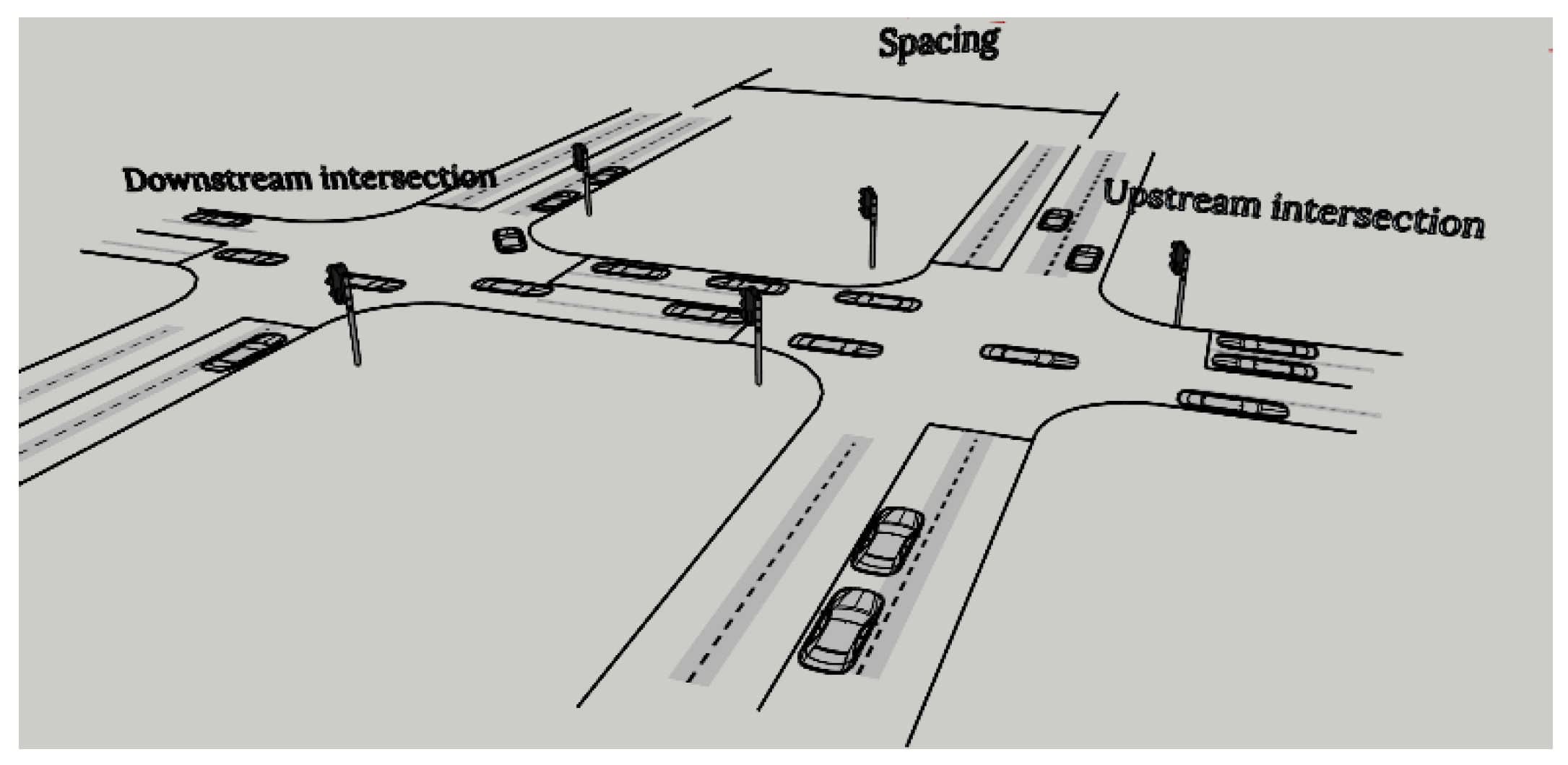
A closely spaced signalized intersection system includes two adjacent signalized intersections. One intersection is referred to as an upstream intersection and the other as a downstream intersection based on the direction of traffic flow (Figure 1). Highway Capacity Manual (HCM) defines the closely spaced intersections as diamond interchanges. Although there is no specifically defined spacing value for the characteristics of closely spaced intersections, the manual defines a range. It is possible to classify intersections that are less than 240 m in distance [28]. The most significant characteristics that differentiate closely spaced intersections are the distance between the two intersections and the queue lengths at the downstream intersection. Delays and queue lengths can be predicted analytically or through simulation using signal cycle parameters, saturation flow, and the maximum traffic volume at the intersection. To ensure effective traffic flow, it is important to estimate the queue length between two intersections under fully saturated conditions. In particular, the queue length should not exceed the spacing between intersections. Therefore, achieving a lower degree of saturation is preferred, and the analyses were conducted within this context [29]. Instead of identifying the optimal spacing between two intersections, it would be more realistic to investigate the threshold value at which the two intersections are considered to be closely spaced by analyzing the factors that influence this determination.

Thanks to advancements in machine learning techniques, it is now possible to focus on traffic fluctuations and simulate their effects in the model [11]. Consequently, new intersection control algorithms are being developed with the help of technology, where the traffic demand is growing daily [30]. A great number of before-and-after case studies on signalized intersections have shown that [23,31,32,33,34] the performance based on queues and delays can be improved by using planning-oriented and operation-oriented approaches [33]. Therefore, installing a signalized system at every intersection may not provide the expected benefits both economically and safely. For this reason, the intersection geometry, signal duration, and associated intersection performance indicators must be determined as accurately as possible.

Delay is one of the traffic performance indicators for evaluating signalization performance, emphasizing the need for minimization [11]. The performance of an intersection cannot be determined solely by delay. It should not be ignored that traffic-related environmental pollution is increasing day by day. CO₂ emissions and fuel consumption rates are exhibiting an increasing trend when intersections are closely spaced. In such scenarios, vehicles often accelerate within a limited distance [13]. As a result, it can be stated that the upstream and downstream performance parameters mutually influence each other in a closely spaced intersection system. If the parameters of the downstream intersection are examined in detail, the offsets, green time, distance from the upstream intersection, average speed of arrival vehicles, and queue lengths have an important impact on the operational characteristics of the upstream intersection, especially for the performance indicator parameter as delay. The operational characteristics of the downstream intersection are essential for calculating the delay [35]. On the other hand, intersections (especially signalized intersections) are the places where transportation-related environmental impacts are most frequently observed. As is well known, intersections are areas in road systems where delays occur and, consequently, the emission of greenhouse gases from vehicles can occur at the highest rates. Due to the potential increase in environmental pollution resulting from increased delay, various studies have been conducted on the environmental impacts of different types of intersections, and particularly numerous studies on signalized intersections are present in the literature [13,36,37,38]. In fuel consumption models, factors such as total traveled kilometers, total delay, and stop rate are considered significant [37]. It is obvious that delay; fuel consumption; noise pollution; and associated psychological, economic, and environmental issues can be observed particularly at signalized intersections [39]. The most effective way to minimize these problems is through accurate and sustainable intersection control strategies. Potential problems of this nature can only be reduced through control strategies by building a sustainable framework.

The aim of sustainable transportation is to preserve the environment and resources while addressing societal needs, alongside evaluating associated benefits and costs. Various studies have demonstrated that the sustainability objectives can be attained in the planning, design, and management of road traffic networks [40]. Previous studies in the literature indicate that fuel consumption models are more strongly correlated with CO₂ emissions than carbon monoxide (CO), hydrocarbons (HC), and nitrogen oxide (NOx). In recent years, there has been a rise in the utilization of emission models, particularly integrated with traffic simulation models [41]. To reflect dynamic traffic behaviors [11], researchers have explored the use of machine learning techniques. The primary advantage of this technique is the ability to capture complex nonlinear relationships between various traffic parameters [42]. Kwak et al. [43] examined the effects of optimizing traffic signal timing on vehicle fuel consumption and emissions in an urban corridor. The optimization was conducted using the TRANSIMS microscopic traffic simulator by integrating the VT-Micro model—a microscopic model for emission and fuel consumption estimation—and a genetic algorithm (GA)-based optimizer for four signalized intersections in Charlottesville, VA, USA. The results were subsequently compared with the optimal traffic signal-timing plan derived from Synchro using the TRANSIMS microscopic traffic simulator. The proposed model significantly outperforms the best Synchro solution in terms of air quality, energy consumption, and mobility metrics, achieving a 20% reduction in network-wide fuel consumption and 8–20% lower vehicle emissions. Guo and Zhang [44] investigated the correlation between environmental impacts and mobility measurements at signalized intersections. This study utilized simulations alongside multivariate multiple linear regression (MMLR) analysis to integrate the microscopic traffic model and estimate traffic emissions. Seven independent variables (control delay, total delay, stops, total stops, average speed, total travel time, and total traveled distance) were selected to assess mobility performance, while seven dependent variables were selected to measure environmental impact. Additionally, a dummy variable was employed to categorize the intersection types. On the other hand, seven dependent variables represent the environmental impact: CO₂, CO, NOx, particulate matter (PM), sulfur dioxide (SO₂), and total energy consumption. The results demonstrated strong correlations across multiple responses.

Lin et al. [42] introduced an integrated approach using artificial neural network (ANN) techniques and Bayesian algorithms to optimize the travel time along a signalized corridor in Ohio. Results indicated that the developed model effectively captures the traffic patterns to calculate the travel time using the ANN–Bayes-trained dynamic profile. Yao et al. [15] developed two single-objective optimization models for paired intersections with uncoordinated and coordinated signals, demonstrating dependencies of green times and left-turn bays on traffic demand. Their results showed that left-turn bays at paired intersections significantly influence operations, particularly under heavy left-turn demand. The findings indicated that coordinated signals outperform uncoordinated ones under moderate traffic demand and spacing but may perform worse under low demand and large spacing. The inclusion of left-turn lanes can improve intersection performance; however, numerous factors, such as intersection geometry, traffic demand, phases, and timing, must be taken into account to optimize their effectiveness across varying traffic periods. Several studies have explored the impact of left-turn lanes on intersection performance, particularly in terms of reducing delays and improving traffic flow. However, limited research has addressed the integration of left-turn-lane length with cycle time coordination by using a machine learning approach. This study aims to reformulate the optimization models for closely spaced intersections by considering left-turn lanes within an integrated research framework. Machine learning models, particularly PLSR [45], PSVM [46], and ANN [47], have an importance in terms of both prediction accuracy and efficiency in predicting traffic flow and fuel consumption. These models allow for the integration of complex, nonlinear relationships between traffic variables, offering a promising approach to optimizing intersection performance, especially under varying traffic conditions. This study presents a novel approach which simultaneously considers both the prediction and integrated optimization framework of length of left-turn lanes and cycle time, offering a more comprehensive approach than previous studies. By using a machine learning-driven prediction and optimization process, this work aims to reflect the dynamic behavior of closely spaced signalized intersections for the literature. Simulations are conducted to evaluate the effects of various influencing factors on traffic flow performance based on fuel consumption. The integration of these factors offers a novel perspective on improving intersection efficiency.

3. Methodology

The proposed study aims to develop a fuel consumption model based on the observed traffic parameters to enhance operational efficiency. The model is generated using a pair of closely spaced intersections that reflect specific urban traffic dynamics. Several parameters were extracted from the video recordings, and the SIDRA model was calibrated based on the observed traffic data. After the calibration and validation process, a series of preliminary analysis were conducted. For the validation process, queue length was selected for similar types of intersections located in İzmir. Several scenarios were created based on the traffic volumes per lane, considering maneuvers such as left turn, and cycle times. To identify statistically significant independent variables, a correlation matrix was used to examine the relationship between the variables. The correlation matrix is a technique used as an initial selection criterion to identify potential input parameters of the model [48]. After determining the statistically significant variables, machine learning techniques were employed to develop a fuel consumption model using PLSR, SVM, and ANN. A wide range of predictive machine learning methods are available in the literature; however, PLSR, PSVM, and ANN were specifically employed due to their strengths in handling multicollinearity, capturing nonlinear relationships, and modeling complex patterns within the data.

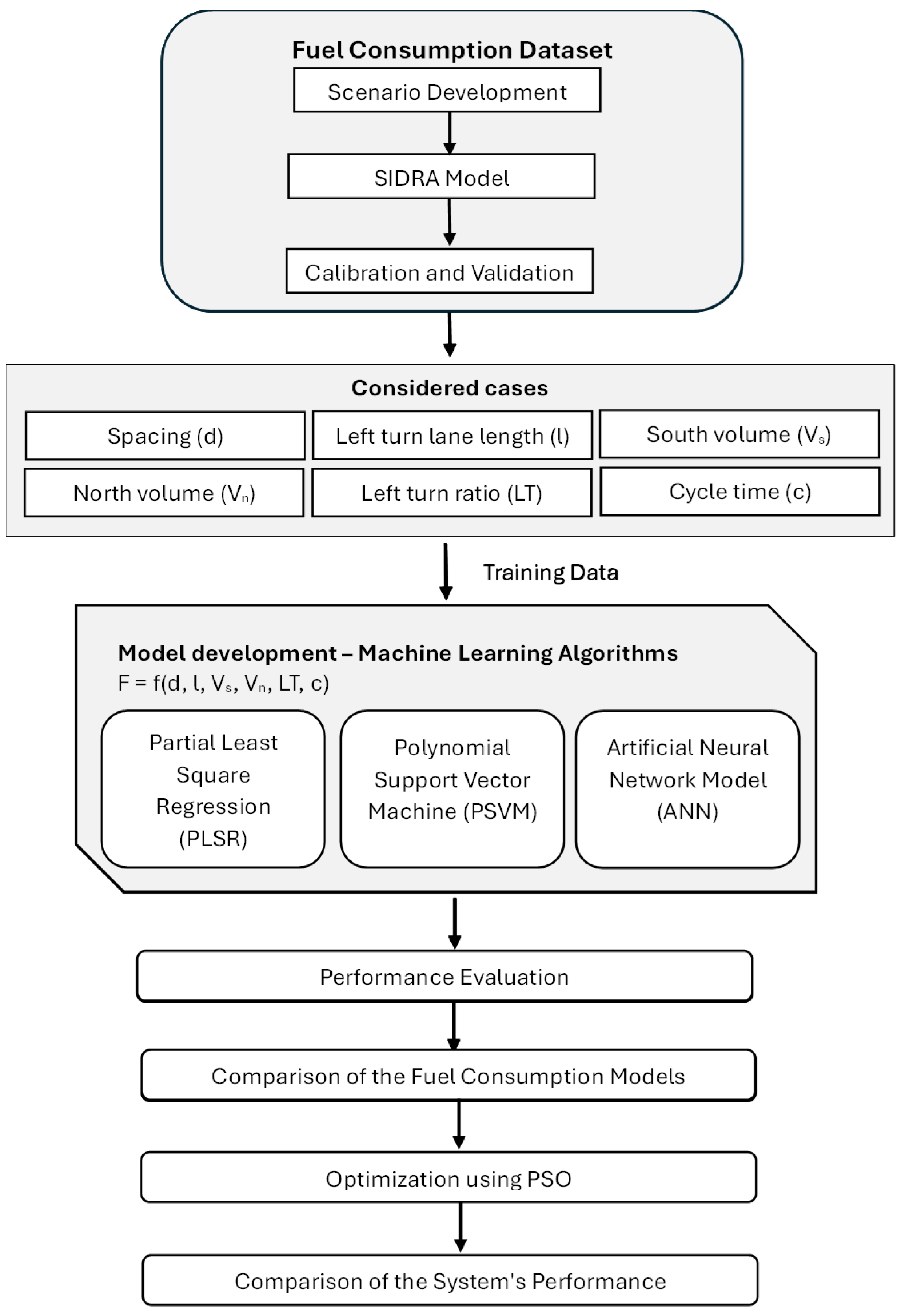
After the evaluation of the performance of each model, one of them is selected to achieve significant improvements in fuel efficiency and overall intersection performance. Cycle time and left-turn ratio are optimized by using PSO, an essential optimization method widely recognized for its efficiency and accuracy in solving complex engineering problems. Figure 2 provides an overview of the model development process for estimating fuel consumption. This comprehensive approach to modeling, optimization, and scenario comparison highlights the novel contributions of this research to the field of urban traffic management and sustainable transportation planning. It can be said that this study focuses on the specific challenges of closely spaced intersections, the integration of advanced machine learning models, the comparative approach, and the innovative application of PSO to optimize intersection parameters. The proposed machine learning framework predicts fuel consumption by considering key factors, facilitating not only a reduction in fuel consumption but also enhancing the environmental effectiveness of traffic management. This approach contributes to the development of sustainable transportation systems.

3.1. Calibration and Validation of the Model

SIDRA Intersection software is preferred as a micro-analytical tool to perform and evaluate lane-based analyses for different types of intersections to conduct the analyses under different traffic conditions [49]. The calibration and validation of the proposed traffic scenarios were implemented based on observed traffic data from Buca and Karabağlar in İzmir, Turkey, focusing on queue lengths. Figure 3a,b show Google Earth views of the studied area. Figure 3c,d illustrate the SIDRA models of the intersections. The Buca intersection system includes two closely spaced signalized intersections, numbered 1 and 2. Similarly, the Karabağlar intersection system comprises two signalized intersections (1, and 2). Considering the distances between all intersections in this system, the spacing between the first and second intersections is compatible with the definition of closely spaced intersections. Therefore, these two intersections were modeled as a system of closely spaced intersections to calibrate and validate the proposed system.

The data collection process presented several challenges due to the complexity of the factors involved. Variations in road conditions and driver behavior posed potential inconsistencies in the data collection procedure, which needed to be carefully validated. For this reason, a camera-based data collection technique was used to provide real-time data [50]. Queue length data for traffic flow were collected using video camera recordings under optimal conditions, including clear weather, good visibility, and the absence of weather-related factors such as wind that could influence traffic patterns or recording quality. Data collection was conducted at 5-min intervals to predict traffic flow, focusing on the morning peak hours from 7:30 AM to 8:30 AM. Instead of relying on human observers, two cameras were installed at each intersection to monitor approaching vehicles and measure queue lengths. The cameras were strategically placed to ensure a comprehensive view of the intersection’s approach area. Vehicle arrivals and departures were recorded following the methodology outlined in [51]. After obtaining the video recordings, the queue lengths were determined by watching the video frames sequentially. Video recording analysts carefully watched the video recordings in five-minute intervals, counting the vehicles of each direction took upon entering and leaving the observed area. Tally counters were used to systematically analyze the count of each vehicle. Analysts also paused, rewound, or slowed down the playback to ensure accurate counting. To enhance the accuracy and reliability of the data collection procedure, different analysts also counted the vehicles from the same video recording. From the video recordings, the number of vehicles stopped during the red phase of each signal cycle was documented, and the queue length was determined by measuring the distance from the stop line to the last vehicle in the queue [36]. To enhance the model’s reliability and accuracy, field data, including traffic volumes, speeds, and queue lengths, were reviewed. Additionally, the cycle lengths and phase timings observed in the field were incorporated into the SIDRA-based model.

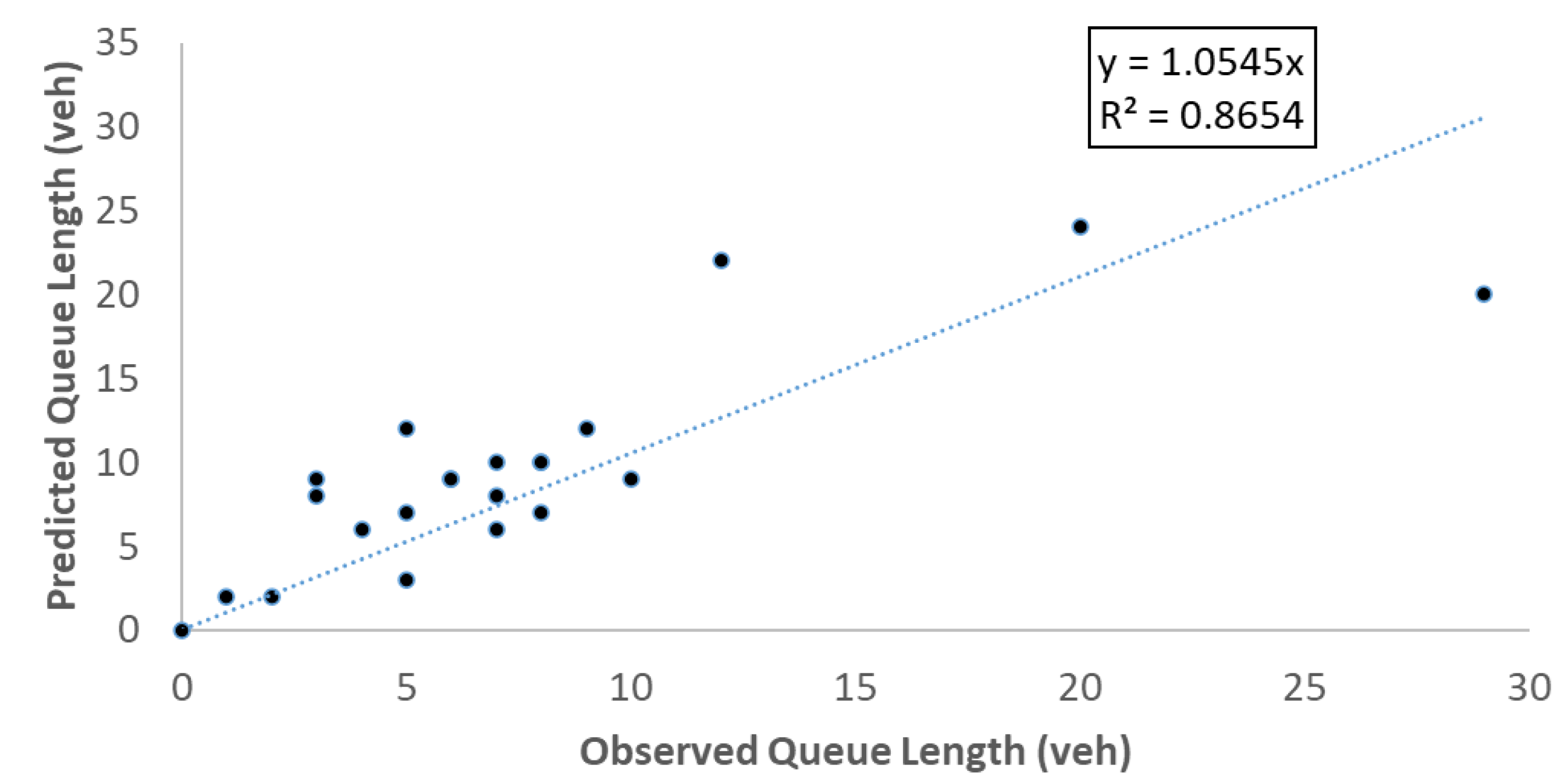
The validation of the proposed SIDRA models was performed using field data as input parameters. Figure 4 compares the queue length values obtained from the simulation, which fits well with the observed values. This is confirmed by the high R² value of 86.54%, indicating that the model accurately represented the observed queue lengths. The difference in queue lengths can be related to the location of the intersection with high pedestrian density in the city center, the geometric characteristics of the intersection, driver and pedestrian behaviors, and the long cycle time. To reflect accurate SIDRA models, road geometric properties, saturation flow, and traffic flow values needed to be assigned. To ensure that the performance values obtained from the program reflect reality, it is necessary to determine the area type factor (ATF) and saturation flow values to be used for each flow. For that purpose, the ATF was used as the saturation flow adjustment factor, which varied between 0.1 and 2 for each approach. According to the empirical model (Equation (1)) obtained from analyses by Bozkurt and Çalışkanelli [52], the ATF values were estimated by setting a saturation flow value of 1950 veh/h. The results were calculated separately for all intersection approaches and entered into SIDRA models [52,53].

$$\mathrm{ATF}=0.0013\ast V_{Total}-2.23488\ast RT-22.8015\ast LT$$

(1)

where V_Total is the total traffic volume, RT is the right turn rate, and LT is the left-turn rate.

3.2. Traffic Scenarios

The main idea of the proposed study is to predict the key performance indicators that significantly influence fuel consumption, particularly in the context of closely spaced intersections, to implement future operational scenarios. Therefore, all necessary traffic and geometric data were carefully examined and modeled in SIDRA, and 137 different scenarios were created to analyze the signalized closely spaced intersections. Each scenario comprises a network of two signalized intersections. Different scenarios were generated by varying the traffic volumes. Categorization and descriptive statistics of the independent variables under different conditions were preferred to evaluate the performance based on low, moderate, and high levels, as can be seen in

Table 1. Classification of explanatory variables.

Parameters	Range	Classification
Spacing between two intersections (d)	50–200 m	Very short	50–100 m
		Short	100–150 m
		Normal	150–200 m
Left-turn-lane length (l)	25–75 m	Short	25–40 m
		Moderate	40–50 m
		Long	50–75 m
The south-approach traffic volume at Site 1 (Vs)	500–2000 veh/h	Low	500–1000 veh/h
		Moderate	1000–1500 veh/h
		High	1500–2000 veh/h
The north-approach traffic volume at Site 1 (Vn)	500–2000 veh/h	Low	500–1000 veh/h
		Moderate	1000–1500 veh/h
		High	1500–2000 veh/h
Left-turn (LT) ratio	5–30%	Low	5–10%
		Moderate	10–20%
		High	20–30%
Cycle time (c)	75–100 s	Actuated	75 s
		Actuated	80 s
		Actuated	85 s
		Actuated	90 s
		Actuated	100 s

. In the created scenarios, the volumes are represented in the range of 500–2000 veh/h. North and south traffic volumes (V_n and V_s, respectively) were categorized as low if the number of vehicles ranged from 500 to 1000 per hour (veh/h), moderate between 1000 and 1500 veh/h, and high between 1500 and 2000 veh/h. Similarly, the spacing between the intersections, denoted by d, was categorized as very short if it is between 50 and 100 m, short for the range between 100 and 150 m, and normal for the range of 150–200 m. Left-turn-lane length (l) was categorized as short for the interval range between 25 and 40 m, moderate if approximately 40–50 m, and long if between 50 and 75 m. Left-turn (LT) rates were categorized as low if between 0 and 5%, moderate if between 5 and 10%, and high if between 10 and 15%.

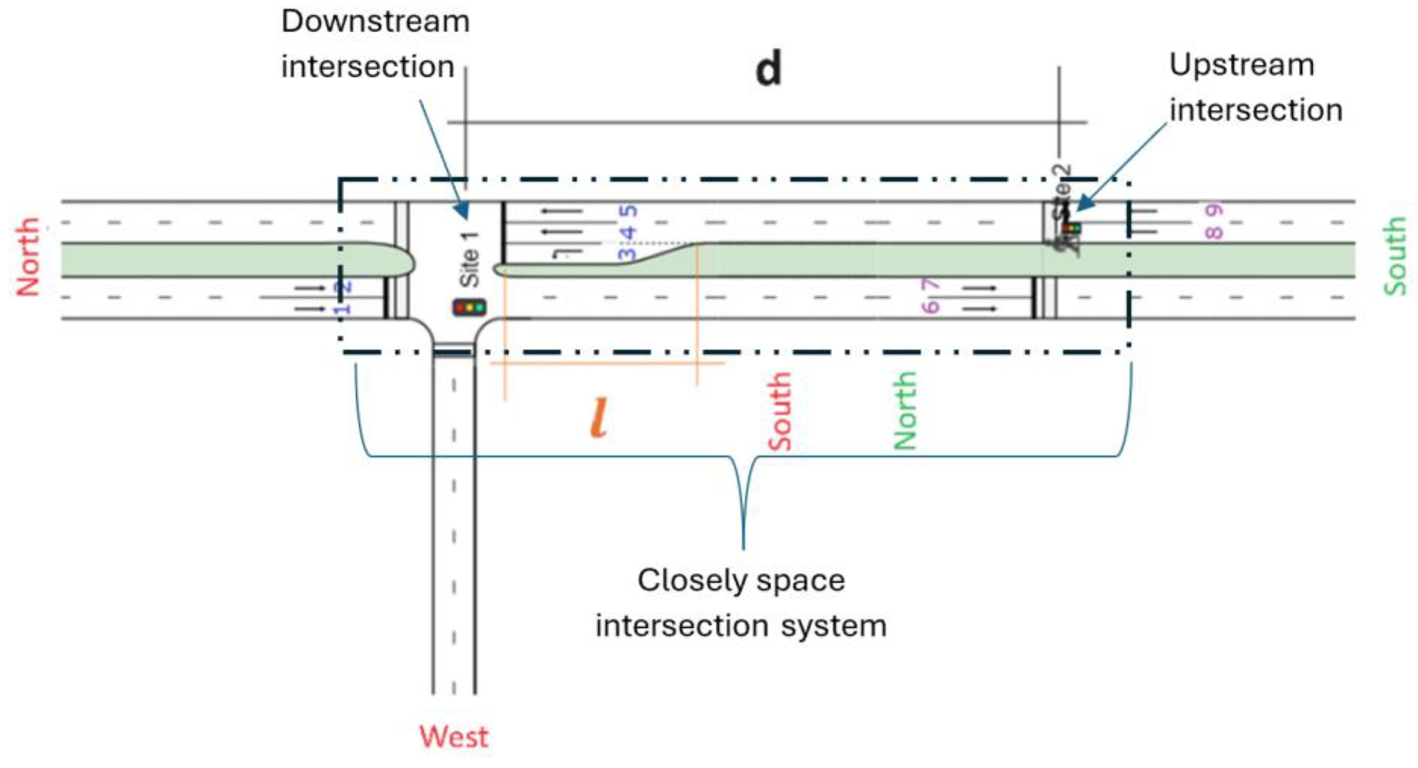
Figure 5 illustrates the western, northern, and southern approaches of the SIDRA model, which consists of two signalized intersections. The south approach of Site 1, which is the downstream intersection, has three lanes (including 1 left-turn lane), while the north approach has two lanes. For the upstream intersection (Site 2), the northern and southern lanes have two lanes. There are a total of 9 traffic flows in the intersection system. Right-of-way information is provided in Phase I of Site 1 for the northern approach, which prioritizes the first, second, third, fourth and fifth lanes. Phase II of Site 1 shows right-of-way is for the fourth and fifth lanes. Phase I of Site 2 includes lanes 6, 7, 8, and 9. An additional phase is allocated for pedestrians.

Fuel consumption is affected by several variables, such as total traveled kilometers, total delay, and stop rate, and can be considered as a complex system [37]. SIDRA performs operational assessments for corridors for various types of intersections and uses a four-mode elemental (modal) model to estimate fuel consumption and pollutant emissions, including CO₂, CO, HC, and NOx. This model calculates fuel consumption and emission values for four driving modes: cruise, acceleration, deceleration, and idling (stopped) time. After the step-by-step estimation of each of the four driving modes, the results are combined to capture the entire driving maneuver from entry to exit. This instantaneous fuel consumption model can be represented using the energy, power, or tractive force necessary for vehicle operation as input parameters. The instantaneous model calculates the fuel consumption rate at any specific moment during the trip, based on the tractive power demanded by the vehicle [54,55]. SIDRA calculates the fuel consumption rate as mL/s by measuring at any instant during the trip, which reflects the tractive power demanded by the vehicle. The instantaneous fuel consumption model is given by Equations (2)–(7) [54].

$$f_t=\left\{\begin{array}{cc}\alpha +{\beta }_1{P}_T+\left[{\beta }_{2}a{P}_l\right]& for P_T>0\\ \alpha & for P_T\le 0\end{array}\right.$$

(2)

$$P_T=\mathrm{m}\mathrm{i}\mathrm{n}(P_{max},P_C+P_l+P_G)$$

(3)

$$P_C={\mathrm{b}}_{1}v+{\mathrm{b}}_1{v}^3$$

(4)

$$P_l={\displaystyle \frac{M_{v}av}{1000}}$$

(5)

$$P_G={\displaystyle \frac{9.81M_v\left(\frac{G}{100}\right)v}{1000}}$$

(6)

$$\alpha ={\displaystyle \frac{f_i}{3600}}$$

(7)

where $f_t$ is the instantaneous fuel consumption rate (mL/s); $P_T$ is the total tractive power (kW); $P_{max}$ as the maximum engine power (kW); $P_c$, $P_l$, and $P_G$ are the cruise, inertia, and grade components of total power (kW), respectively; and G is road grade (%). $M_v$ represents the total vehicle mass (kg), $v$ is the instantaneous speed (m/s), and $a$ is the instantaneous acceleration (m/s²). $\alpha$ is the constant idle fuel consumption rate (mL/s) applicable to all driving modes. $f_i$ demonstrates the idle fuel consumption rate, indicating the amount of fuel consumed by a vehicle’s engine while idling (mL/h). Different vehicles have varying engine efficiencies and fuel consumption characteristics. For instance, passenger cars generally have a lower $f_i$ compared to heavy vehicles. SIDRA uses calibrated $f_i$ values for specific vehicle categories, derived from field measurements or manufacturer data [56,57]. Two vehicle parameters are used in Equation (4): ${\mathrm{b}}_1$ as parameter related to the rolling resistance (kN), and ${\mathrm{b}}_2$ as aerodynamic drag parameter (kN/(m/s)²). In addition, ${\beta }_1$ is used as an efficiency parameter related to the fuel consumed to the total power provided by the engine (mL/kJ), and ${\beta }_2$ is used as an as efficiency parameter to reflect the fuel consumed during the positive acceleration (mL/(kJ.m/s²) [54].

The instantaneous cruise fuel consumption rate ($a$ = 0, $P_I$ = 0) on a level road ($G$ = 0, $P_G$ = 0) is determined using Equations (8)–(12). These formulations focus solely on cruise conditions. The parameter units are specified as mL/m for $c_1$ and (mL/m)/(m/s)² for $c_2$ [54].

$$f_{ct}=\alpha +{\beta }_1{P}_C$$

(8)

$$f_{ct}=\alpha +{\beta }_1\left({\mathrm{b}}_{1}v+{\mathrm{b}}_2{v}^3\right)$$

(9)

$$f_{ct}=\alpha +c_{1}v+c_2{v}^3$$

(10)

$$c_1={\mathrm{b}}_1{\beta }_1$$

(11)

$$c_2={\mathrm{b}}_2{\beta }_1$$

(12)

Equation (10) plays an important role in the model calibration process for fuel consumption. Once the parameters $c_1$, $c_2$, and ${\beta }_1$ are determined through calibration, the subsequent model parameters are calculated and serve as the input parameters of the model ($A$ and $B$ parameters, Equations (13) and (14), respectively).

$$A=1000c_1$$

(13)

$$B={\displaystyle \frac{c_2}{0.01296}}$$

(14)

where $A$ is known as the drag fuel consumption parameter, mainly related to rolling resistance (mL/km); and $B$ is called the drag fuel consumption parameter, which is mainly related to aerodynamic drag (mL/km)/(km/h)². The parameters ${\mathrm{b}}_1$ and ${\mathrm{b}}_2$ are calculated indirectly using the $c_1$ and $c_2$ values, which are determined for fuel consumption based on Equation (15) and Equation (16), respectively. This is performed to provide a realistic representation of the drag (cruise) power required from the engine. Additionally, ${\mathrm{b}}_1$ and ${\mathrm{b}}_2$ account for certain components of drag related to the engine [54]. These parameters are provided in

Table 2. SIDRA fuel consumption model parameters [57].

Parameters	Units	For Light Vehicles
$f_i$	mL/h	1200
A	mL/km	16
B	(mL/km)/(km/h)2	0.004
${\mathrm{b}}_1$	kN	0.16
${\mathrm{b}}_2$	kN/(m/s)2	0.000518
${\beta }_1$	mL/kJ	0.100
$M_v$	kg	1600

for light vehicles [56,57].

$${\mathrm{b}}_1=\left\{\begin{array}{c}{\displaystyle \frac{c_1}{{\beta }_1}} if {\beta }_1>0\\ 0 if {\beta }_1=0\end{array}\right.$$

(15)

$${\mathrm{b}}_2=\left\{\begin{array}{c}{\displaystyle \frac{c_2}{{\beta }_1}} if {\beta }_1>0\\ 0 if {\beta }_1=0\end{array}\right.$$

(16)

3.3. Parameter Selection

The correlation matrix of the studied variables was created using the Python environment to analyze the interactions between fuel consumption (L/h) and selected parameters [58]. The correlation matrix aims to identify the most significantly relevant variables and investigate the relationship between fuel consumption and these independent variables. Six key performance parameters were selected as independent variables, which are given in Table 1. Pearson’s correlation coefficient was used to evaluate each independent variable [59], as shown in Figure 6. The correlation matrix values vary between −1 and +1. Values close to −1 are interpreted as negative correlations, and values close to +1 are interpreted as positive correlations with strong relationships. There is no correlation between these two variables for values close to 0 [59,60]. The intensity of the red color in Figure 6 indicates that there is a positive relationship between the variables, whereas the blue intensity indicates an inverse relationship. It is possible to say that the parameter most related to fuel consumption (F) is the volume of the north (V_n) and south (V_s) approaches, with correlation values of 0.68 and 0.63, respectively. Thus, volume is one of the most important parameters in the model and can be considered to provide good correlation.

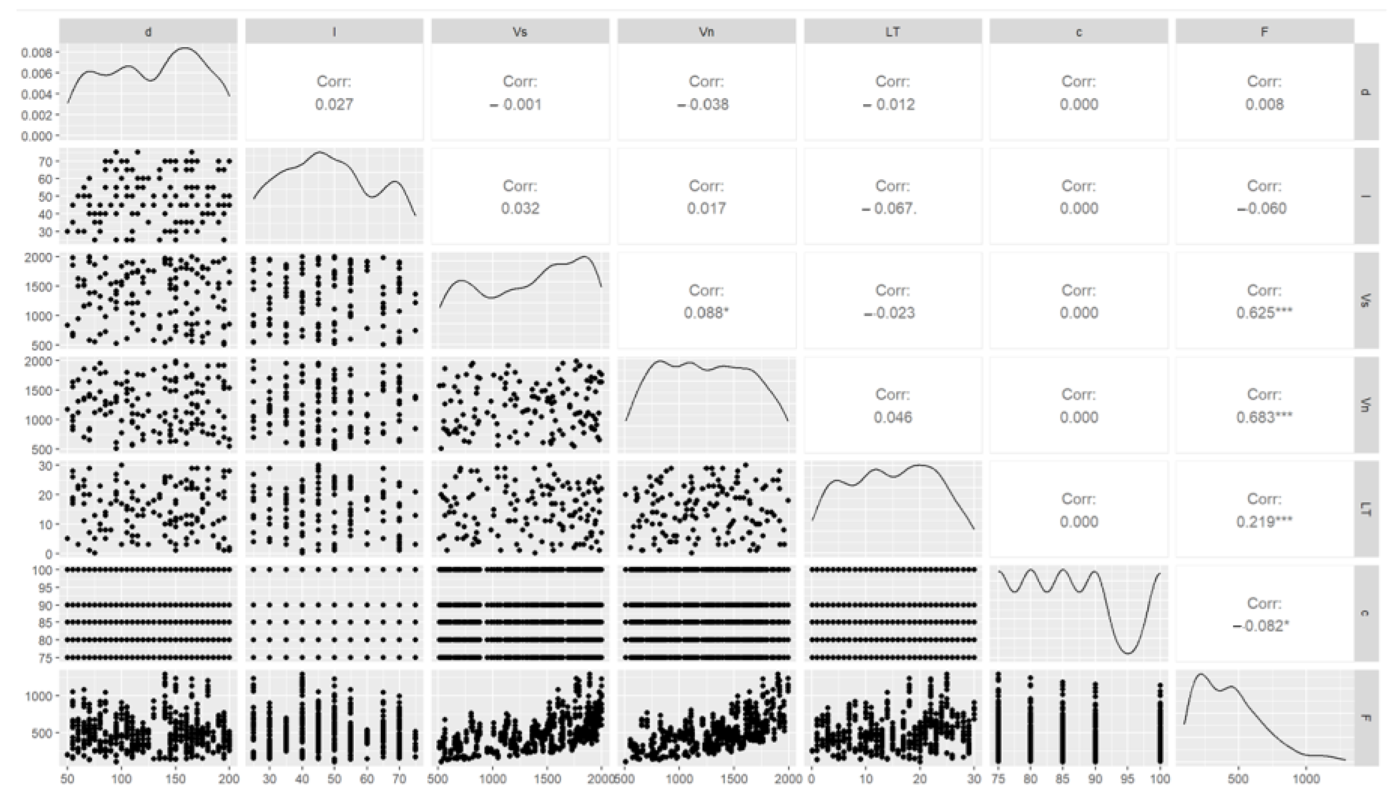
The pair plot of the dependent and independent variables used in the analysis were again visualized in R, as shown in Figure 7. This method combines a correlation matrix and a scatter plot that represents the frequency distribution of all parameters on the diagonal to visually assess the relationships between variables. Each cell in the graph represents the relationship between two variables as a correlation matrix. Scatter plots are displayed in the lower part of the diagonal, while the Pearson correlation coefficient between two variables is presented in the upper part by the “Corr” label, which indicates the strength and direction of the correlation. The strong correlation between V_n and vs. is represented by 0.683 *** and 0.625 ***, respectively. Therefore, the effect of volume on fuel consumption needs to be considered. The low negative correlation between fuel consumption and cycle time (Corr: −0.082 *) is an indication to consider which denotes a weaker correlation. Each cell contains scatter plots showing the distributions of the two variables. The more scattered plots did not show a clear relationship. It can also be explained by their corresponding low correlation coefficients.

3.4. Model Development

The average number of stops is an important metric for evaluating the performance of signalized intersections. It is obvious that an increase in the number of stops results in higher fuel consumption and emissions [61]. This situation is particularly possible at closely spaced intersections. For this reason, the research question has evolved significantly to reflect the parameters required to minimize fuel consumption, depending on different traffic volumes, spacings, cycle times, and left-turn maneuver parameters for closely spaced intersections. In this context, machine learning techniques are aimed at modeling the fuel consumption of closely spaced intersection systems. Thus, these models can serve as a promising method for predicting the fuel consumption of closely spaced intersection networks.

After determining the parameters used as dependent and independent variables in the model to predict the fuel consumption values (defined in Table 1), the following measures were selected to compare the accuracy of the machine learning models. Following the selection of the parameters, the models are trained in several steps. PLSR is the first model trained, where dimensionality is reduced while maximizing variance in predicting fuel consumption. The second model, PSVM, is trained by adjusting the kernel function and polynomial degree to capture nonlinear relationships. The third model, ANN, is developed by tuning the architecture, including the number of layers and neurons, and training using backpropagation. Once the models are trained, a comparative analysis is conducted to evaluate the performance of PLSR, PSVM, and ANN. Performance indices include R² and RMSE, as well as execution time and computational efficiency for each model. The development of reliable generative models relies on precise performance evaluation. Incorporating a confidence interval (CI) allows for the assessment of uncertainty in error estimates and model performance. By using confidence intervals, upper and lower bounds can be calculated, providing a range within which the actual error is expected to lie [62].

The RMSE is a commonly used statistical measure to evaluate the fit of regression models. It predicts the inconsistency between the observed and corresponding predicted values, which can be seen in Equation (17) [11,63]. R² emphasizes the strength of the relationship between input and output variables, which can be seen in Equation (18). For all equations, n denotes the number of observations, y_i denotes the observed fuel consumption values, z_i represents the predicted values as the outputs of the machine learning models, and $\overline{y}$ represents the mean observed fuel consumption [11].

• Root mean square error (RMSE):

$$RMSE=\sqrt{{\displaystyle \frac{\sum _{i=1}^n{\left(y_i-z_i\right)}^2}{n}}}$$

(17)

• Coefficient of determination (R²):

$$R^2=1-{\displaystyle \frac{\sum _{i=1}^n{\left(y_i-z_i\right)}^2}{\sum _{i=1}^n{\left(y_i-\overline{y}\right)}^2}}$$

(18)

Consequently, the spacing, left-turn-lane length, traffic volumes, and left-turn rate were adjusted, either increased or decreased by certain percentages, at each intersection approach, resulting in the creation of 137 different scenarios for five different cycle times, which were converted to 685 different datasets. To consider the dynamic nature of traffic flow and the interactions between adjacent intersections, the fuel consumption was modeled using the PLSR, SVM, and ANN algorithms. In this section, the algorithms considered in this study are briefly discussed.

After comparing the models, PSO is employed to optimize parameters such as left-turn-lane length and cycle time to minimize fuel consumption. The performance index for this step is the percentage improvement in fuel consumption from the optimized parameters. Finally, model validation is performed under varying traffic conditions to assess how the final model (with optimized parameters) performs across different scenarios.

3.4.1. Partial Least Square Regression (PLSR) Model

A simple method to gain an idea about the factors that may affect fuel consumption is to perform a PLSR analysis. PLS regression analysis is conducted using the nonlinear iterative partial least squares (NIPALS) or PLS-KERNEL algorithm. NIPALS forms the foundation of PLS regression. The goal of this algorithm is to identify the components that maximize the covariance matrix. During each iteration, a single component and its weight and loading values are determined. The process continues until the desired number of components is obtained [64]. Its ability to handle multicollinearity of the independent variables [64] while reducing the dimensionality [65] makes PLSR well-suited for predicting the relationships of the simulation dataset. However, it can be difficult to assess the complexity of traffic parameters in a way that effectively captures their dynamic effects. Therefore, additional machine learning methods are explored to better capture these uncertainties.

3.4.2. Support Vector Machine (SVM) Model

The SVM is an essential tool for classifying and fitting data. It is a supervised learning algorithm applicable to both classification and regression problems [66]. The fundamental concept of SVM involves creating one or multiple hyperplanes in a high-dimensional space, which can be used for classification, regression, or other tasks. The SVM algorithm identifies a hyperplane in an N-dimensional space (where N represents the number of features) that effectively differentiates between data points [67,68]. The SVM algorithm can be used on both linear and nonlinear datasets by using the kernel parameter [69]. SVM is highly effective in regression tasks and performs well even with nonlinear relationships between the variables, which is important in traffic optimization scenarios where interactions between variables like traffic volume, cycle time, and intersection distance are complex [70]. Additionally, it is also proven that the polynomial model reflects better fuel consumption than linear, making it suitable for the predictions. It has been observed that fuel consumption predictions can be expressed with more complex models instead of linear models [68].

3.4.3. Artificial Neural Network (ANN) Model

The ANN is a computational model that imitates biological neural networks. Owing to its reliability and flexibility, the model can be used in all fields, including engineering and research [48]. The traffic patterns can be learned and mimicked by the model using the ANN method, which can be described as a smart algorithm [42]. Due to its capacity to model highly nonlinear relationships and interactions between multiple factors in traffic systems, where factors exhibit complex and nonlinear patterns, the ANN method is used; it serves as a flexible and powerful tool to capture these relationships [48].

Network architectures, node characteristics, and learning methods are the fundamental structure of an ANN. An artificial neural network is created by the interconnection of artificial neurons. The model includes three layers: (1) input layer, (2) at least one hidden layer, and (3) an output layer. The main processing units of a neural network are called nodes [48]. The intermediate nodes between the input and output layers can form one or multiple hidden layers. Each neuron is linked to all neurons in the subsequent layer. The input layer gathers information from external sources, the hidden layer processes this information, and the output layer generates predictions [71].

The inputs are multiplied by a modified weight. The transmission of the inputs is performed by a transfer function that creates the output of the neurons. The optimal number of hidden neurons can be determined in trials to achieve the highest determination coefficient and lowest MSE between the observed and predicted data [48]. Each neuron in the hidden layer is associated with a weight vector, W, representing synaptic connections to the input layer and bias value, b. The output neuron corresponding to the number dependent variable is connected to all hidden neurons. The signals from the hidden layer were multiplied by the output neuron weight, W, and adjusted by the bias. The aggregate signal transmitted to the neuron serves as the input to an activation function specific to that neural layer [63]. A graphical representation of the proposed ANN model structure is presented in Figure 8.

3.4.4. Particle Swarm Optimization (PSO)

PSO, a metaheuristic algorithm, is particularly effective for addressing nonlinear and non-convex optimization problems. It is inspired by the collective behavior observed in animals, such as schools of fish and flocks of birds. In this approach, potential solutions for an optimization problem are represented by particles located within the design space. In each generation, each particle adjusts its position according to both its own best position and the best position found by the entire swarm [48]. The particles move through the N-dimensional problem space, learning from the historical data of all other particles. It is an iterative approach where the position of particle i at iteration t + 1 is updated based on Equations (19) to (22) [72,73]:

$${\mathit{V}}_i^{k+1}=w\ast {\mathit{V}}_i^k+c_1\ast ran{d}_1\ast \left({\mathit{P}}_{i,best}^k-{\mathit{X}}_i^k\right)+c_2\ast ran{d}_2\ast \left({\mathit{G}}_{i,best}^k-{\mathit{X}}_i^k\right)$$

(19)

$${\mathit{X}}_i^{k+1}={\mathit{X}}_i^k+{\mathit{V}}_i^{k+1}$$

(20)

$${\mathit{P}}_{best}^{k+1}=\left\{\begin{array}{cc}{\mathit{X}}_i^{k+1}& if f\left({\mathit{X}}_i^{k+1}\right)<f\left({\mathit{P}}_{i,best}^k\right)\\ {\mathit{P}}_{i,best}^k& if f\left({\mathit{X}}_i^{k+1}\right)\ge f\left({\mathit{P}}_{i,best}^k\right)\end{array}\right.$$

(21)

$${\mathit{G}}_{i,best}^{k+1}=min\left\{f\left({\mathit{P}}_{0,best}^k\right),\dots ,f\left({\mathit{P}}_{n,best}^k\right)\right\}$$

(22)

In this context, V and X represent the velocity and position of the particles, respectively. X_i is also called the mapping coefficient parameter for the ith vector. The parameter k denotes the iteration number; and c₁ and c₂ are constants which are referred to as the cognitive and social factors. P_i,best is the best position found within the neighborhood of particle i as the personal experience. G_i,best is the best position discovered across the entire particle population. The random values between 0 and 1 are rand₁ and rand₂, and w is the inertia factor [72,74]. The fitness function is denoted by f, which is used to assess how close a solution is to the optimal one by evaluating the P_i,best and G_i,best. Lastly, n refers to the total number of mapping coefficient vectors, commonly referred to as the swarm size [73].

Researchers focused on new heuristic and meta-heuristic intelligent algorithms for delay models like differential evolution algorithm (DEA), artificial bee colony (ABC) [75], genetic algorithm (GA), particle swarm optimization (PSO), flower pollination algorithm (FPA) [76], fuzzy logic (FL), and so on [77]. PSO is well-known for its ability to achieve a good balance between exploration (searching new areas of the solution space by fast convergence) [47] and exploitation (refining known solutions) [78]. This is particularly beneficial for complex optimization problems, where the solution space is large and multi-dimensional, and both global and local search capabilities are important [74]. Since traffic systems are often subject to a high level of complexity and nonlinearity, PSO’s global search capability makes it well-suited for finding optimal solutions [78].

4. Results and Discussion

All the necessary parameters for implementing the PLSR, SVM, and ANN methods were determined through multiple iterations and were incorporated into the models presented in

Table 3. Algorithm configurations of the model implementation.

Algorithm	Analysis Methods
PLSR	Fit method	:	Kernelpls
SVM	Fit method	:	Kernel function
	Function type	:	3rd order polynomial
	Epsilon	:	0.1
ANN	Training algorithm	:	Levenberg–Marquardt
	Activation function of hidden layer	:	tansig
	Activation function of the output layer	:	purelin
	Number of hidden layers	:	1
	Number of neurons in hidden layer	:	8
	Number of iterations (epochs)	:	100
	Learning rate	:	0.01

. The algorithms were implemented using Minitab, MATLAB, and R programing language. The dataset is provided as the input to the models for performing the machine learning algorithms. The input data are divided into three parts: training, testing, and validation. Generally, 70% of the dataset was used for training, 15% was reserved for testing, and 15% was reserved for validation. The outputs of the algorithms generate the fuel consumption predictions. The test and validation data were evaluated by using the trained algorithms. The results obtained were compared according to their performance metrics.

4.1. PLSR Model

The proposed PLSR model is useful for working with multiple dependent variables and high-dimensional datasets. The models were used to predict dependent variables based on independent explanatory variables, using the partial least squares assumption. The model was randomly split into datasets, using 70% training, 15% testing, and 15% validation to ensure the model’s validity.

Table 4. PLSR model training variance-explained ratio results.

Components	X	F
1	54.84	77.86
2	99.39	79.52
3	99.88	80.41
4	99.95	83.75
5	99.98	84.77
6	100.00	84.78

presents the variance-explained ratios of independent variables (X) and dependent variables (F) for each number of components as input parameters. These ratios indicate how well the model explains the data. According to the table, the variance-explained ratio for fuel consumption with five components is 84.77%, and with six components, it is 84.78%. This indicates that the model can capture 84.77% of variability in dependent variable F by adding five components into the model. Using six components in the model slightly improves the model’s explanation of variance by 84.78%. The increase in variance explained from 84.77% to 84.78% after adding one additional component is very small. Thus, the gain of the model’s explanation is minimal. However, the variance-explained ratio of X with 1 component is 54.84%. The model explains 100% of the total variance using six components. In other words, the model captures all variability in independent variables using these six components.

The regression relation obtained from the PLS regression is presented as follows:

$$F=-276.575+0.201d-1.295l+0.300V_s+0.373V_n+5.936LT-2.299c$$

(23)

According to Equation (23), it can be predicted that the spacing between closely spaced intersections, the left-turn ratio, and the volumes of the south and north approaches have positive effects on fuel consumption. On the other hand, as the left-turn-lane length increases, the fuel consumption also decreases. The main factor is the reduction in the queue spilling over from the left-turn bay, which decreases the likelihood of obstructing vehicles moving through the bay. As a result, the reduction in the number of stops can contribute to a decrease in fuel consumption. 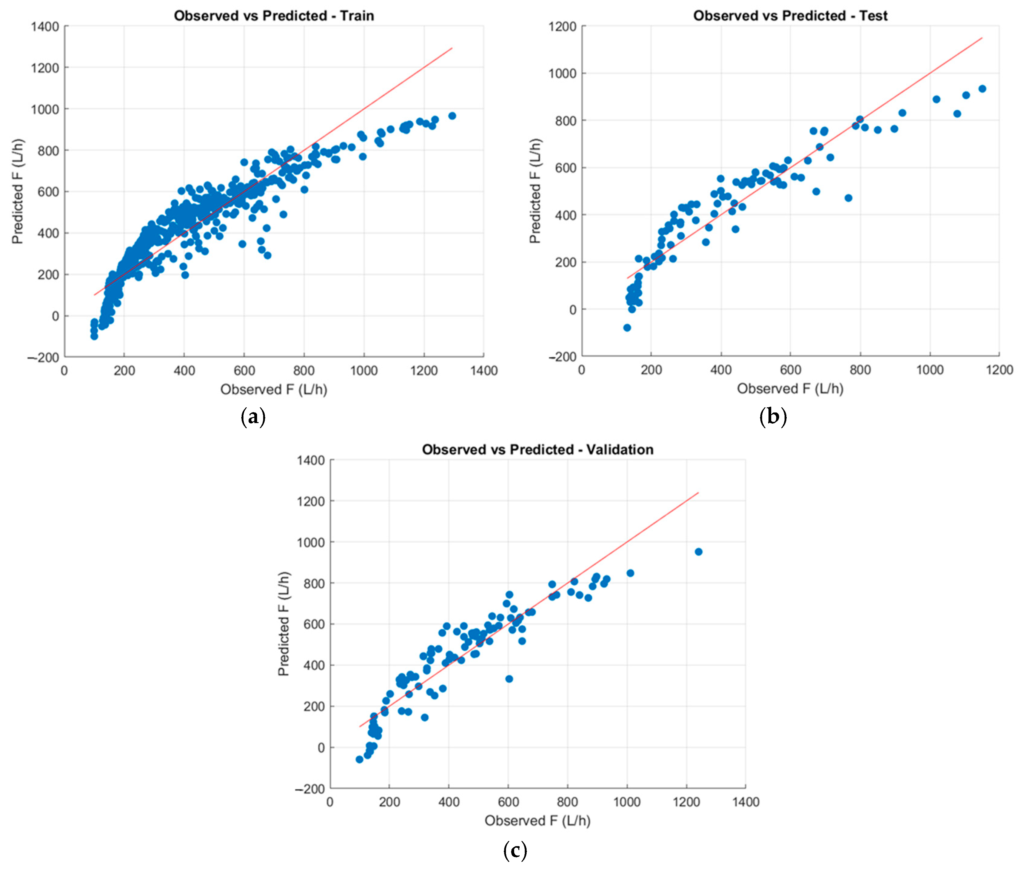The regression fit between the predicted and actual fuel consumption values using the PLSR model is shown in Figure 9. Figure 9a shows the dataset with 70% training, while Figure 9b shows the 15% testing set. Figure 9c shows the best fit during the validation phase. The skewness observed in the data indicates that the model did not yield accurate results. Therefore, other models are desired to be implemented.

4.2. SVM Model

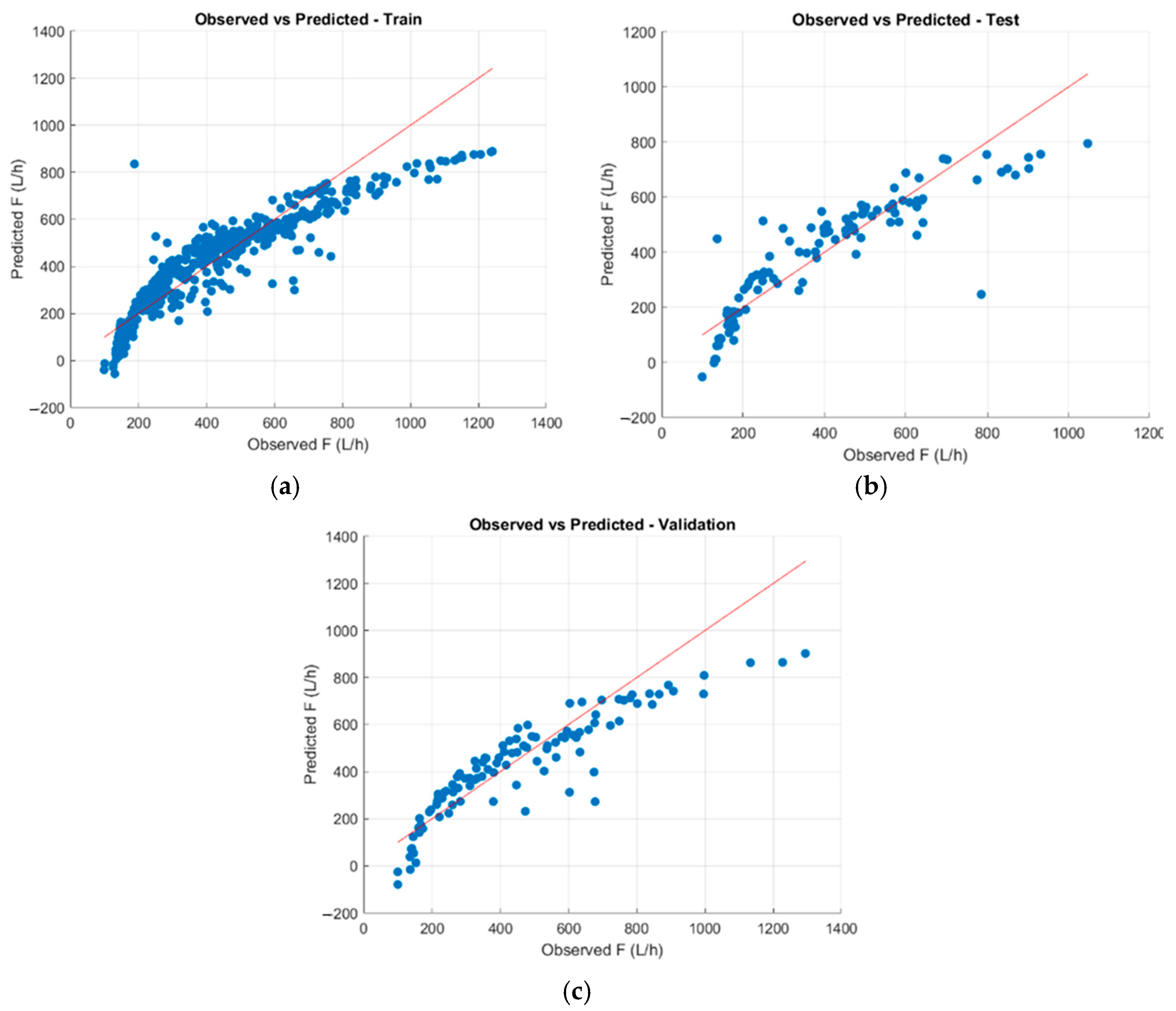
Among the four commonly used kernels for SVM models—linear, polynomial, radial, and sigmoid—[68] employed, we chose to use linear support vector machine (LSVM) and polynomial support vector machine (PSVM) models to identify effective hyperplanes for predicting fuel consumption. Figure 10 and Figure 11 show the regression fits of the LSVM and PSVM models, respectively. Figure 10a presents the training set, Figure 10b demonstrates the test results, and Figure 10c displays the validation set of the LSVM method. 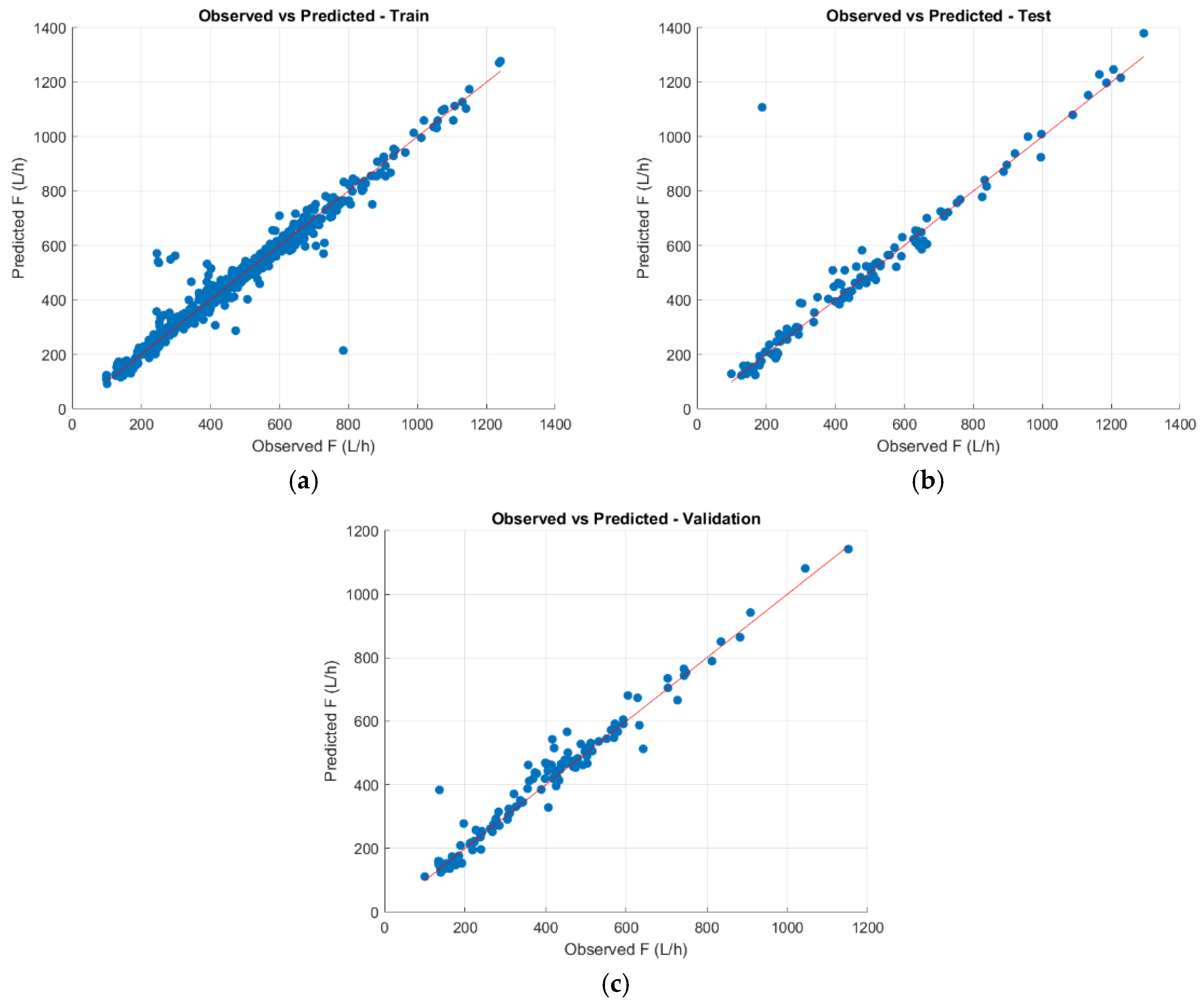The related metrics (R²) were 0.818, 0.775, and 0.786 for training, testing, and validation, respectively. It is important to note that the accuracy of prediction for the LSVM models was approximately 79%, whereas the PSVM model achieved accuracy of approximately 96%, which is considerably higher. It can be deduced that fuel consumption along the corridor of a closely spaced signalized intersection, based on the key influencing factors, is likely to be established by a nonlinear relationship rather than a linear relationship. The outputs of the same parameters obtained from the PSVM method yield more accurate results. The results are presented in Figure 11, where Figure 11a shows the training set with an R² value of 0.977, Figure 11b illustrates the test set with an R² value of 0.935, and Figure 11c displays the validation set with an R² value of 0.967. Therefore, the PSVM method was selected within the scope of the study as an algorithm for comparison.

4.3. ANN Model

The learning process of an ANN model begins by generating datasets using a mechanism that mimics input–output relationships. During this process, the input data are multiplied by weights, added to the previous input node, and stored in a hidden layer. In the final stage, the model computes the prediction errors by comparing the actual output with the predicted output. The backpropagation process iteratively monitors and adjusts the weights backward to gradually minimize the error [68].

To evaluate the ANN model, first, the database of the explanatory (independent) variables and fuel consumption as dependent variables were used to train and test the model in MATLAB2024a. Various models were created and assessed using different methods and architectures. The primary objective is to develop predictive models that minimize residual errors using various algorithms [79]. To select an appropriate training algorithm for the ANN control parameters, Levenberg–Marquardt and Bayes regularization training algorithms were examined, respectively, taking into consideration other studies in the literature [25,42,48,60,63,80]. To identify the best model, the dataset was divided into training, testing, and validation subsets (70% for training, 15% for testing and 15% for validation).

After deciding to examine these two algorithms in this study, the number of hidden layers and number of neurons were investigated. The selection of hidden layers and neuron numbers was undertaken to determine the optimal ANN model by using Levenberg–Marquardt and Bayes regularization algorithms. The code was executed to find the optimal ANN architecture with the number of hidden layers ranging from 1 to 10 and the number of neurons in each layer ranging from 1 to 20. For each configuration, performance was evaluated on both the training, test, and validation sets, and the model with the best validation MSE was selected. In addition, the best model is saved for utilization purposes. According to the results obtained for the models, Levenberg–Marquardt was chosen as the training algorithm due to its high speed and suitability for efficiently generalizing large datasets to solve the drawbacks of backpropagation algorithms. The optimal ANN architecture model is presented in

Table 5. Optimum architecture information of the ANN model.

Input Layer		Hidden Layer		Output Layer
Independent Variables (Predictors) (Explanatory variables)	Spacing between intersections Left-turn-lane length South approach traffic volume at Site 1 North approach traffic volume at Site 1 Left-turn ratio Cycle time	Number of hidden layers	1	Dependent Variable (Response)	Fuel consumption
		Number of neurons in the hidden layer	8
		Activation function	Hyperbolic tangent sigmoid transfer function (tansig)	Activation function	Linear transfer function (purelin)

. The size of the hidden layer was determined numerically by minimizing the RMSE value to obtain the most precise possible model. For accurate prediction by the ANN model, training was conducted multiple times, with a configuration of six input layers corresponding to independent variables, one hidden layer, and one output layer, as depicted in Figure 8. The optimal architecture is represented by 6-8-1. The input layer consists of six neurons according to the number of input features (number of independent variables) fed into the model. The neural network with one hidden layer attained a satisfactory level of accuracy. Eight neurons indicate the number of neurons in the hidden layer. The input layer processes the inputs using weights and biases. The neurons in this layer apply an activation function to introduce nonlinearity, which allows the network to learn complex patterns, where one denotes the number of neurons in the output layer. This represents the final output of the model that reflects the single dependent variable as fuel consumption. The proposed architecture obtained the best overall results in training, testing, and validation. In the model, the Levenberg–Marquardt training algorithm is used by the feed-forward method, with the hyperbolic tangent sigmoid transfer function (tansig) of the hidden layer and linear transfer function (purelin) of the output layers to account for most of the model fit to predict fuel consumption.

The structure of the ANN model is presented in Figure 8. A well-structured artificial neural network can then provide accurate predictions using new input data [71]. According to the three layers of the model (input, hidden, and output), the formulas for the outputs of the hidden layer ($s_j$) and output layer ($y_k$) can be seen in Equations (24) and (26), respectively. Here, variable n represents the number of input variables, m represents the number of neurons in the hidden layer, and p denotes the number of neurons in the output layer. The i-th input of the input layer is represented by x_i, where w_ij is the weight of the i-th input to the j-th input of the hidden layer. The weight that connects the j-th output of the hidden layer to the k-th input of the output layer is indicated by $w_{jk}$; ${\theta }_i$ and $b_k$ signify the biases of the hidden and output layers, respectively; $\varnothing \left(x\right)$ specifies the activation function of the hidden layer, while $\psi \left(x\right)$ refers the activation function of the output layer; $s_j$ describes the output of the hidden layer; and $y_k$ expresses the output of the output layer [81].

$$s_j=\mathrm{\varnothing }\left(\sum _{i=1}^n\left(w_{ij}\ast x_i\right)+{\theta }_i\right)$$

(24)

$$y_k=\psi \left(\sum _{j=1}^m{w}_{jk}{s}_j+b_k\right)$$

(25)

$$y_k=\psi \left(\sum _{j=1}^m{w}_{jk}\mathrm{\varnothing }\left(\sum _{i=1}^n\left(w_{ij}\ast x_i\right)+{\theta }_i\right)+b_k\right)$$

(26)

The feed-forward neural network training process of the Levenberg–Marquardt algorithm effectively minimizes errors within a relatively short period. The model with the optimal hidden layer and neurons produced significantly accurate estimations. Figure 12 illustrates the relationship between the training data of the ANN model and the actual fuel consumption. It can be clearly observed that ANN predictions closely match the actual values. Correlation coefficient, R, was determined for training, testing, validation, and all estimated high values (around 0.97). In addition, very few points were located far from the line representing the perfect fit (Y = T).

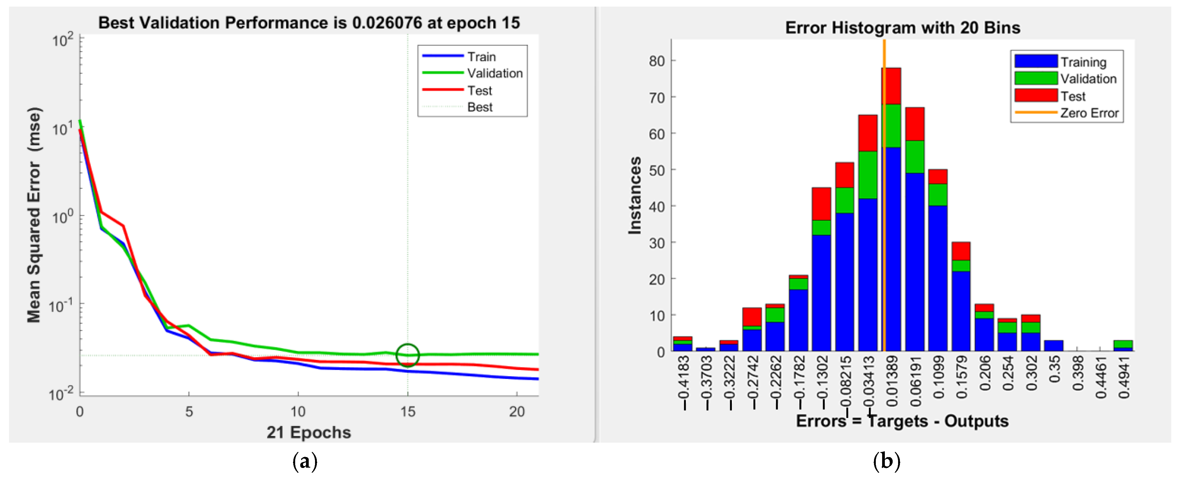
The network was trained in 15 epochs of learning, as shown in Figure 13a, by achieving a normalized MSE for the validation set equal to 0.026076, as highlighted in the graph with a circle around the point of its best validation performance. The reduction in MSE in the initial epochs demonstrated for all three sets (training, validation, and test) that the model is learning and improving its performance quickly during the early stages of training. The training (blue) and test (red) curves continued to decrease slightly after epoch 10, indicating that the model improved on the training and test data. However, the validation (green) curve remained relatively flat, suggesting that beyond epoch 10, additional training did not lead to significant improvements in the validation performance. The error histogram is represented in Figure 13b, which was created by the model of three sets of data: training, validation, and testing. It is an important graph to evaluate the model’s performance. The errors in the training, test, and validation sets are shown in blue, green, and red, respectively. The graph displays the distribution of differences between predicted and actual values as errors. The errors were concentrated near zero. It can be stated that the model was effectively trained, and the model generally made accurate predictions. The error distribution is symmetric. Therefore, there was no systematic bias in the model’s predictions. The zero-error line (orange line) indicates that the model generally makes accurate predictions. According to these graphs, it can be concluded that the model performed well.

4.4. Comparison of the Models

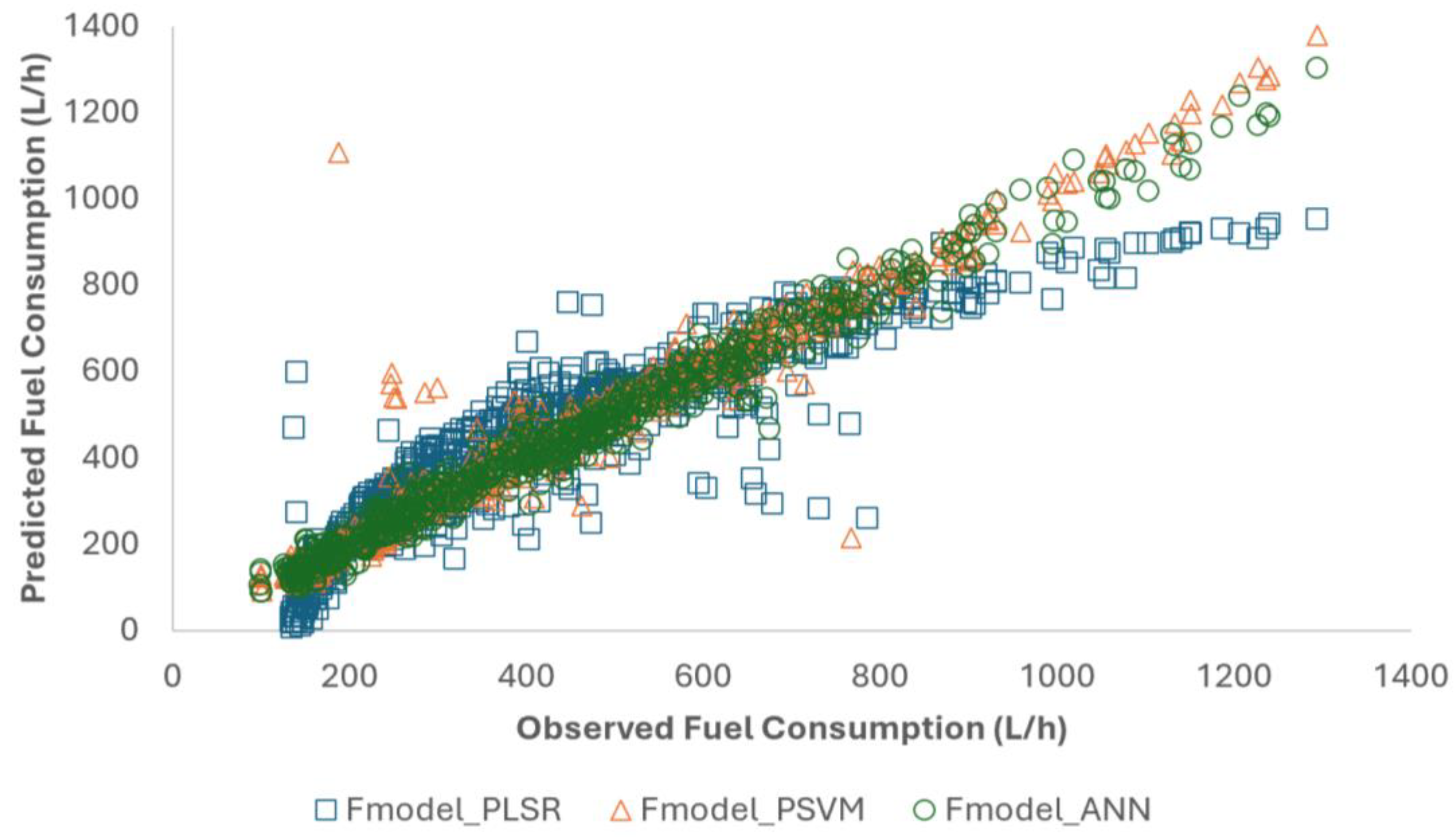
Overall assessment (Figure 14) revealed that the PLSR model does not serve as a generalized model. The PSVM and ANN plots better reflect the total model. Similarly, their training, testing, and validation fit results are better. It is aimed at capturing the model’s predictive accuracy by using RMSE. To strengthen the results with statistical validation, the R-squared value is also computed. Moreover, a 95% confidence interval was obtained by estimating the mean of RMSE based on the range of the populations generated during the model training, validation, and test process [62]. The lower limit (LL) and upper limit (UL) values of 95% CI are given. A Z-score of 1.96 was used to calculate the 95% confidence interval [82]. According to the performance metrics listed in

Table 6. Performance comparison of the developed PLSR, SVM, and ANN models.

Metric		Method	PLSR	PSVM	ANN
RMSE		Train	92.42623	41.18593	23.06229
		Test	91.12188	61.18592	37.91553
		Val.	108.30013	42.87474	44.51378
CI	LL	Train	84.15765	37.50138	20.99911
	UL		100.69481	44.87048	25.12547
	LL	Test	82.96999	55.71214	34.52356
	UL		99.27377	66.65970	41.30750
	LL	Val.	98.61145	39.03911	40.53152
	UL		117.98881	46.71037	48.49604
R2		Train	0.84780	0.97745	0.99021
		Test	0.85300	0.93538	0.99385
		Val.	0.81962	0.96737	0.98613
Elapsed Time (s)		Training	7.83	6.32	5.92
		Process	0.12	0.10	0.02

Note: Training: This process occurs during the presentation of datasets for training networks, where adjustments are made based on network errors. Validation: The datasets were employed to assess the generalizability of the artificial neural network and terminate its training when generalization did not demonstrate improvement. Testing: The datasets were independent of the network training process. It was used to evaluate model performance during and after training [80]. UL = upper limit; LL = lower limit of 95% of confidence interval.

, PSVM’s regression plot (Figure 11) during the training phase provided satisfactory results. However, during testing, the R² value was less than that of the other sets. Table 6 presents the RMSE and R² values of the models. The proposed ANN model in this study delivers the most accurate predictions compared to the other methods. The lower and upper limits of 95% of confidence intervals results show that the PLSR model exhibited the widest interval (for training, 84.158–100.695), reflecting greater uncertainty in its predictions for training, test, and validation sets. The ANN model demonstrated the narrowest confidence interval (20.999–25.125), indicating the highest reliability in its predictions, indicating its robustness to changes in datasets. The narrower confidence intervals of the ANN model indicate its ability to provide more accurate and reliable predictions. Training time indicates the duration it takes for the model to learn from the data. The PLSR model has the longest training time, which suggests it may involve a more complex structure or require more computations. The ANN model has the shortest training time, which may indicate a more efficient learning process. Process time refers to the time required for the trained model to make predictions on new data. The ANN model has the lowest processing time, indicating that it can generate predictions much faster than the other models. Based on the elapsed times provided, the ANN model is likely the most efficient in terms of both training and prediction speed.

4.5. Sensitivity Analysis and Visualization with Partial Dependence Plot

Following the development of the models, sensitivity analysis is employed to evaluate the impact of variations in input parameters on the model’s output [83]. It is an important method to understand how variations in specific input parameters affect the model’s results and performance. This analysis is often used to evaluate model performance and identify the effects of the most critical parameters. It is essential to assess the generalized capability of the obtained models to examine the effects of variables on fuel consumption. The six independent variables are distributed within a range of ±10%. In each analysis, while one independent variable is used in its distributed form, five other variables are kept constant in each simulation. Thus, the extent to which the independent variable affects the output of the PLSR, PSVM, and ANN models can be determined [84].

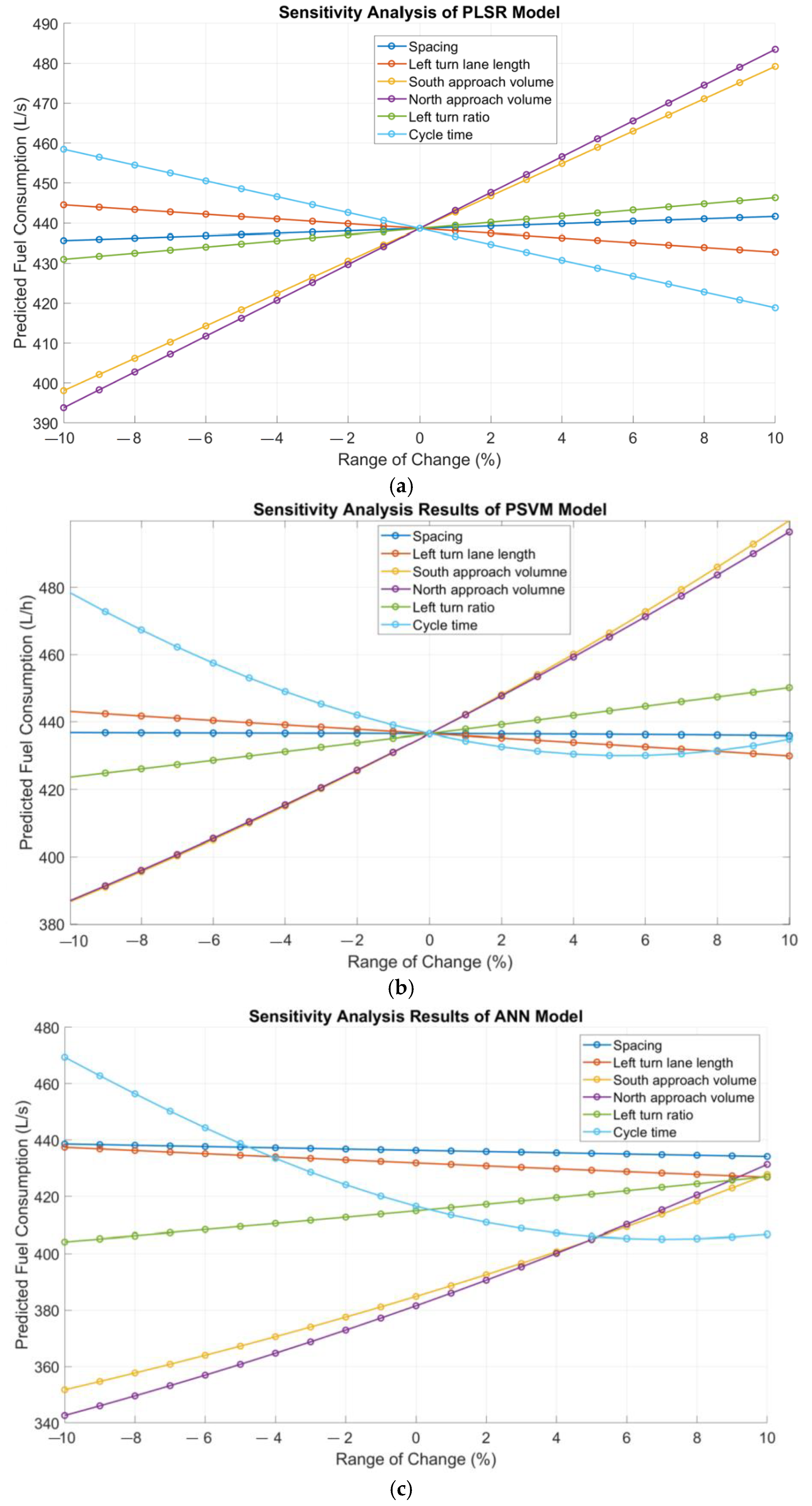
The results of the gradual change in the six input variables used in the proposed models are shown in Figure 15, which presents important information. The effects of the independent variables on the fuel consumption of the PLSR, PSVM, and ANN models are shown in Figure 15a, Figure 15b, and Figure 15c, respectively. The x-axis represents the percentage values of the parameter being varied, while the y-axis gives the corresponding predictions. Linear sensitivities were obtained for the PLSR model, whereas curvilinear sensitivity variations were observed for the PSVM and ANN models. For the spacing parameter, significant predictions were not observed across the three models. The average prediction to consider the effect of left-turn-lane length remains relatively stable until a change in approximately 6% is applied. After this point, a decrease in the trend can be examined. The graph indicates that the prediction is not very sensitive to changes in the left-turn-lane length. For the south and north approach volumes, significant changes occur when the range of change is adjusted to within 10%. As the traffic volumes on the south and north approaches increase, fuel consumption also rises. This indicates that volumes have an increasing effect on the model’s predicted value. Therefore, it is obvious that when the number of vehicles within a closely spaced intersection increases, traffic-related fuel consumption also increases. This will also lead to traffic congestion between the two intersections, causing vehicles to stop and resulting in delays. The graphs demonstrate that the average prediction is highly sensitive to changes that can occur for the cycle time when it increases. A sharply decreasing trend is highlighted for cycle time, and the model remained relatively stable at approximately 410 L/h. The minimum value can be observed between the three models’ predictions.

Due to the significance of cycle time as a key parameter observed from the sensitivity analysis, a partial dependence plot (PDP) was created to examine the relationship between cycle time and other variables in detail. PDPs were used to visualize the relationship between predictors and responses. It represents the marginal effects of the features on the output using the Monte Carlo method [85]. PDPs can illustrate how the factors impact the predicted outcome of a machine learning model. Consequently, PDP is used to investigate the relationship between fuel consumption and cycle time at closely spaced intersections. The model predictions are calculated for all possible values of a specific independent variable, while the other variables are held constant [86]. 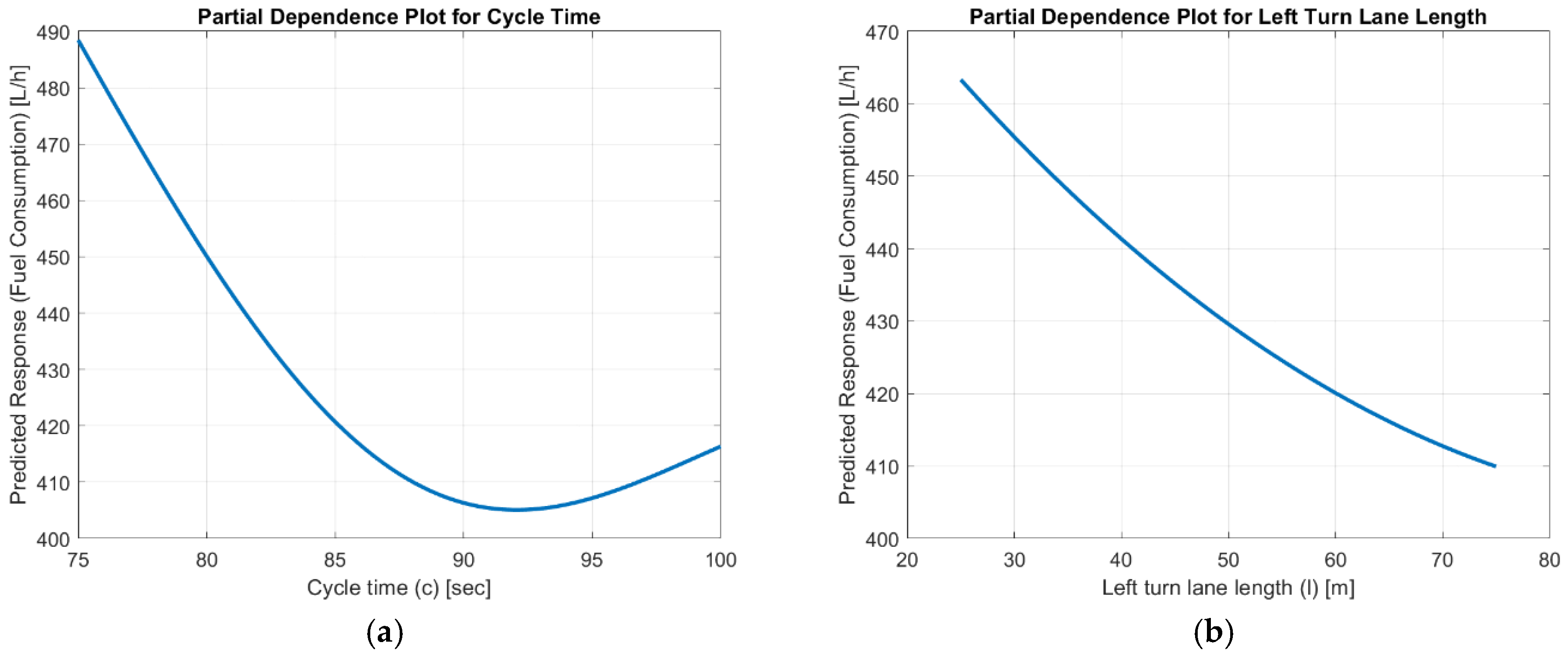PDP isolates and visualizes the effect of a specific variable on fuel consumption [87]. The effect of cycle time according to the ANN model predictions of fuel consumption is shown in Figure 16a. The plot reveals the relationship between cycle time and fuel consumption predicted by the ANN model, with cycle times between 90 and 95 being the most significant. The graph shows that fuel consumption reaches a minimum value when the cycle time of the closely spaced intersections is approximately 92 s. This point can be considered the optimal cycle time, as it corresponds to the lowest fuel consumption. The effect of left-turn-lane length according to the ANN model can be seen in Figure 16b.

The plot shows the relationship between the left-turn-lane length (l) and the fuel consumption. As the left-turn-lane length increases from 25 m to 75 m, the predicted response decreases, indicating an inverse relationship between the two variables. Specifically, as the lane length increases, the response decreases steadily, which could suggest that a longer left-turn lane reduces fuel consumption, improving traffic flow. But here, it should be emphasized that such a long-left-turn lane cannot be observed because even the spacing between intersections is not this long enough to handle it.

4.6. Graphical Representation of Model Predictions

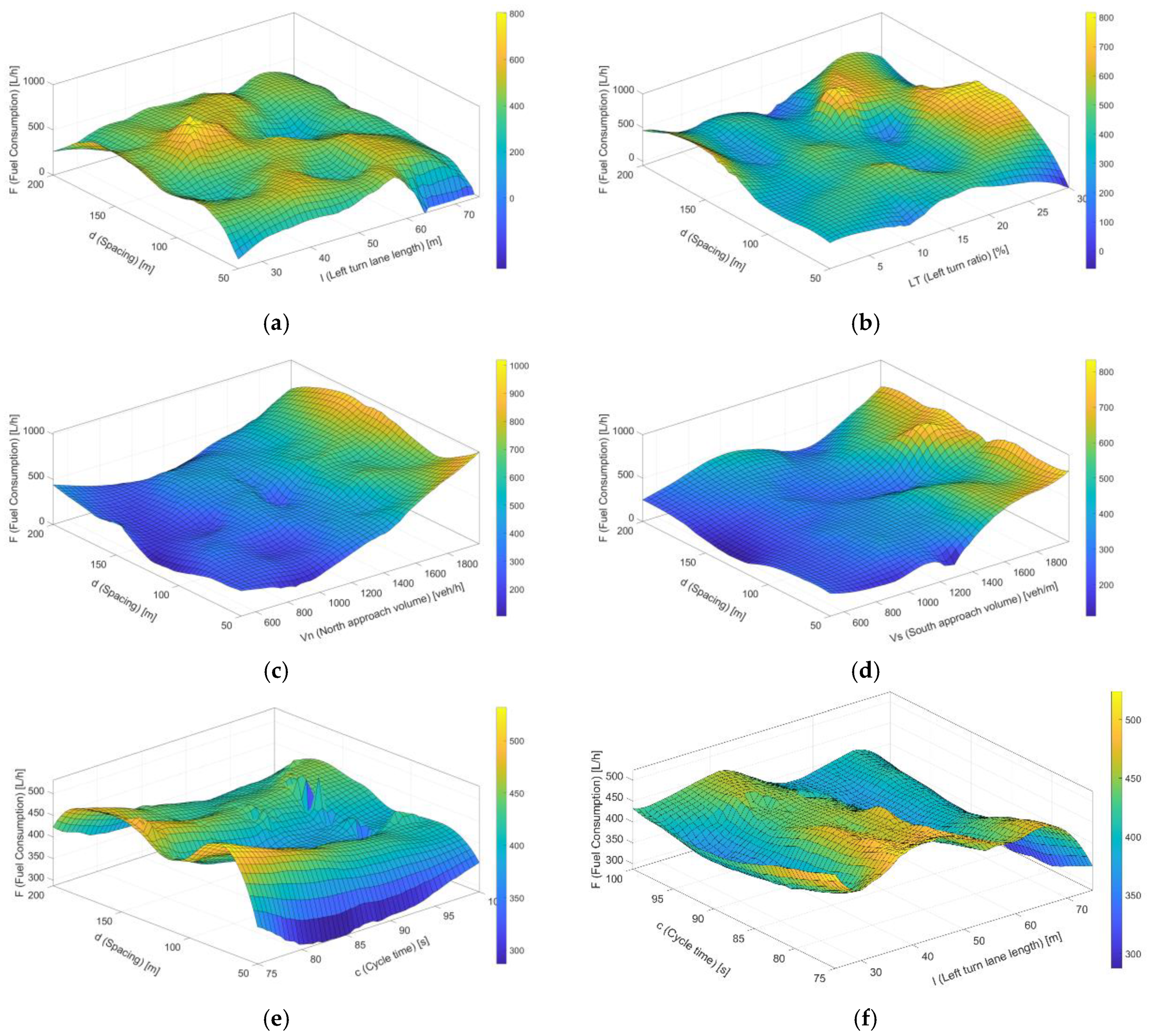
A specific focus was placed on examining the effect of each parameter with fuel consumption model predictions. If we particularly wanted to examine the effect of cycle time with respect to the spacing parameter for the fuel consumption model, a slight decrease in fuel consumption can be observed when the cycle time increases. On the other hand, fuel consumption is not very sensitive to the spacing parameter, as shown in Figure 17. The figure shows the effect of spacing (d) and cycle time (c) on fuel consumption (F) in liters per hour. The fuel consumption varies nonlinearly with both the spacing and cycle time. For low spacing values when the cycle time value increases, the fuel consumption rate of the closely spaced intersection system also increases. However, for larger spacing values, the fuel consumption increased as the cycle time increased. The graphs show the variations in two parameters based on the ANN fuel consumption model predictions. Figure 17a shows the effects of the spacing and left-turn-lane length on fuel consumption. The x-axis shows the spacing between the intersections, ranging from 50 to 200 m. The y-axis shows the left-turn-lane length. The z-axis represents the predicted fuel consumption. For low-spacing values between two intersections, the fuel consumption was maintained steadily without any noticeable change up to a lane length of 60 m. After this point, when the left-turn-lane length increases, the fuel consumption also decreases. However, when the spacing values were between 100 and 150 m, the fuel consumption decreased. A similar tendency can also be observed in Figure 17b for left-turn ratios up to 25%. For approximately 120 m, when the left-turn ratio is high, fuel consumption significantly decreases. However, when the spacing is shorter, a downward trend in fuel consumption can be predicted. Figure 17c,d represent the effects of volume with spacing. The color transition in the graph shows that lower volumes within a range of spacing values are associated with lower fuel consumption, whereas higher volumes correspond to higher fuel consumption.

As the number of vehicles entering the intersection increases, it is obvious that this increase will have a negative effect on fuel consumption. A similar effect can be seen clearly also for 120 m. There is fluctuation in Figure 17e for the combined effect of cycle time and spacing. A significant increase in fuel consumption can be observed for sections with shorter cycle times. A reduction in fuel consumption is specifically observed within the range of 100–150 m regardless of the cycle time. Here, the observed decrease was consistently observed across the range of spacing values. This range can be considered an important scale for the spacing parameter. The same effect can be seen in Figure 17f, where the cycle time and left-turn-lane length are functions of fuel consumption. The graph shows considerable fluctuations. However, nearly 60 m of the left-turn-lane length can be observed in a transition region where the fuel consumption slightly decreases. The decrease is more pronounced for 90 s of cycle time. A substantial increase in fuel consumption is observed when the left-turn ratio increases by up to 25%, which can be seen in Figure 17g. After this range, a reduction in fuel consumption is specifically observed. The joint effect of fuel consumption volumes is examined in Figure 17h. A sharp increase in fuel consumption is observed with an increase in both fuel volumes.

4.7. Development of a Fuel Consumption Model Based on Optimization of Left-Turn-Lane Length and Cycle Time with PSO

To understand the capability of the introduced ANN model, the PSO algorithm is used to address an optimization of cycle time and left-turn-lane length. The proposed PSO-ANN integration focuses on enhancing traffic signal-control strategies at intersections. The primary objective is to reduce fuel consumption, thereby improving traffic flow and efficiency. Therefore, the optimized cycle time and left-turn-lane length determined by PSO are utilized. The results exhibit suitable fitness when compared to the SIDRA model results. PSO is performed by using MATLAB2024a. The configuration of the PSO model can be seen in

Table 7. Configurations of PSO algorithm.

Parameters	Value
Particle swarm size	50
Max iterations	100
Inertia weight (w)	0.7
Cognitive constant (c1)	2
Social constant (c2)	2

. This optimization operates in an open-loop framework, focusing on predefined conditions without dynamic adjustments [88], whereas a closed-loop system would involve real-time feedback to refine decision-making based on actual traffic conditions [89]. In the case of PSO used to optimize left-turn-lane length and cycle time, the optimization is performed with predefined parameters, without observing the system’s reactions or changes; instead, it focuses on optimizing system parameters under a given set of conditions to reveal the applicability of the PSO-ANN system.

The parameters of PSO are critical for balancing exploration (global search) [47] and exploitation (local search) [78]. The swarm size (number of population) typically ranges from 20 to 50 particles for most problems, though larger swarms may be needed for high-dimensional problems [90]. Cognitive constant (c₁) controls the influence of a particle’s own best-known position. Social constant (c₂) determines the influence of the swarm’s global best position. A higher value promotes convergence toward the global best [73]. Common values for c₁ and c₂ are between 1.5 and 2. In this research, values between 0.4 and 0.9 were used to assess the sensitivity of the inertia weight [91].

This inertia weight of the particles is typically represented by random numbers, which generally fall within the range of 0 to 1 [74]. For PSO parameter selection, an adaptive PSO was used, where parameters such as the w, c₁, and c₂ were dynamically adjusted during the optimization process. In this approach, the parameters were initially set for exploration (larger values for c₁, c₂, and inertia weight) and gradually reduced over time to enhance exploitation and refine the search for optimal solutions. This adaptive adjustment allows the algorithm to efficiently balance exploration and exploitation, improving the optimization performance.

For a more detailed and comprehensive analysis, the optimal left-turn-lane length and cycle time values were determined based on three distinct traffic volume ranges, low (500–1000 veh/h), medium (1000–1500 veh/h), and high (1500–2000 veh/h), in order to identify the ideal ranges for each parameter with three different spacing intervals (0–50 m, 100–150 m, and 150–200 m). After determining the optimized values for c and l, scenarios were created and stored by replacing c and l with the optimized results using the same dataset. A comparison of original fuel consumption results obtained from SIDRA (original cycle time and left-turn-lane length) and improved fuel consumption results (optimized cycle time and left-turn-lane length using the PSO-ANN model) for the closely spaced intersection system can be seen in Figure 18.

Table 8. Optimized c and l for different traffic volume and spacing obtained by PSO.

Vs (veh/h)	d (m)	Optimized l (m)	Optimized c (s)	Average Improvement Rate based on Spacing (%)	Average Improvement Rate Based on Volume (%)	Average Improvement Rate of the Network (%)
500–1000	50–100	30	85	8.4	10.7	8.9
	100–150	50	90	8.6
	150–200	30	85	15.0
1000–1500	50–100	40	90	3.9	7.3
	100–150	40	95	8.8
	150–200	65	95	9.3
1500–2000	50–100	50	90	5.2	8.8
	100–150	55	95	3.8
	150–200	40	90	17.5

presents the optimal c and l values, and each combination of these parameters corresponds to a specific improvement rate (%) value for evaluating the performance metric. As the volume of the southern approach is categorized into low, medium, and high traffic volumes, a significant reduction in fuel consumption is observed with the help of the optimized cycle time and left-turn-lane length. In general, the d = 150–200 range tends to have the highest percentage improvement values, with 15.0% for Vs = 500–1000. Shorter distance ranges (50–100) tend to have lower relative improvement, especially for higher volume ranges (1000–1500 and 1500–2000). Longer distances (d = 150–200) generally lead to higher performance gain, particularly at lower volumes. However, for higher volumes, the distance impact is less pronounced. Specifically, a reduction of 10.7% in fuel consumption was noted in the low volume range, 7.3% in the medium volume range, and 8.8% in the high-volume range. However, the overall intersection fuel consumption rate has improved by 8.9%.

Figure 18 illustrates the relationship between spacing (d) and improvement rate (%) for different traffic volumes (V_s) of improved results. At low traffic volumes (V_s = 500–1000 veh/h, represented by blue line), the improvement rate remains relatively constant as spacing increases, indicating that the effect of spacing on improvement is minimal. For medium traffic volumes (V_s = 1000–1500 veh/h, represented by orange line), the improvement rate increases with spacing, but the rate of increase is slower compared to higher traffic flow scenarios. At a higher volume of traffic flow (V_s = 1500–2000 veh/h with green line), the enhancement increases significantly with increased spacing, highlighting that spacing has a more pronounced effect under higher traffic conditions.

The range actually indicates an enhancement, as observed with the PDP, between 85 and 95 s, which can be seen in Figure 19a. However, it is difficult to make a similar statement for l, as it should be smaller than the spacing between the intersections. Figure 19b represents the typical values after optimization.

4.8. Key Findings and Implications

The essential findings and their impact are discussed in the following summary. All machine learning models showed good results, but the ANN model achieved the highest performance. This model offers a simple and easily applicable method for estimating fuel consumption by considering several key influencing factors. Furthermore, a sensitivity analysis was conducted to emphasize the possible performance limits of the proposed models. These models are sensitive to variations in some input variables, which directly affect fuel consumption at closely spaced signalized intersections. For this purpose, the optimization of the most influential parameters was performed, and a PSO-ANN model was developed, aiming to calculate the values that will minimize fuel consumption.

PSO was chosen because of its simplicity; ability to handle complex, high-dimensional problems; and previous successful application in similar optimization problems. These characteristics make PSO an ideal choice for minimizing fuel consumption at closely spaced intersections in the study. The hyperparameters of the ANN and PSO models were selected by identifying the best configuration. These values were determined by testing different configurations in preliminary experiments. By providing these specific hyperparameter values, it can be ensured that the results can be reproduced by other similar studies.

The applicability of this system is quite broad, especially in transportation systems. Specifically, the methods used in this study, such as machine learning algorithms (ANN, PLSR, and PSVM) and PSO, are highly applicable to real-world traffic management systems. The system can be applied to closely spaced intersections in urban environments, where optimizing traffic signal timings and left-turn-lane length to reduce fuel consumption can lead to improved air quality, reduced congestion, and better overall traffic flow. With the increasing integration of Internet of Things (IoT) technologies in smart cities, this framework can be used for real-time traffic monitoring and dynamic optimization of signal timings based on traffic volume, distance between intersections, and other influencing factors. At the same time, by minimizing fuel consumption and reducing carbon emissions, this approach contributes directly to the creation of more sustainable transportation systems.

5. Conclusions and Recommendations

An increase in the average number of stops leads to higher fuel consumption and emissions. This effect is more likely to occur when the distance between two intersections is reduced and is particularly common at closely spaced intersections. As a result, the research question has evolved significantly to address which parameters affect the minimization of fuel consumption based on varying traffic volumes and left-turn ratios at closely spaced intersections, as well as identifying the key factors influencing the development of a fuel consumption model using three different machine learning algorithms to attain an efficient method. It is expected to achieve at least 80% prediction accuracy for determining fuel consumption. A series of analyses were conducted using partial least squares regression, support vector machine, and artificial neural network algorithms, and an evaluation of their respective performances was performed. These methods were chosen because each method complements the others in handling different aspects of the data—such as dimensionality, nonlinearity, and complexity—while improving the accuracy of the predictive model. Independent variables affecting fuel consumption were included as inputs of the model for training the system. All machine learning models yielded promising results; however, the ANN model performed better by demonstrating the best performance.

In addition, a sensitivity analysis was carried out to highlight the potential performance limits of the proposed models. Cycle time is particularly sensitive and exhibits a negative trend, which indicates that it directly influences the fuel consumption reduction. This is likely related to the decrease in the average number of stops during longer cycle times and potentially extended green phases, thus helping to avoid queueing problems. The length of the left-turn lane exhibited the second highest sensitivity to fuel consumption, showing a relatively strong negative correlation with fuel consumption reduction. In contrast, other variables affect fuel consumption, showing a trend where increases in these variables lead to higher fuel consumption. Spacing had a minimum effect on fuel consumption and exhibited relatively low sensitivity. This analysis identifies the variables that are critically important to the system, and it is necessary to focus on these variables to make potential improvements. To reflect the capability of the introduced ANN model, the PSO algorithm is used for optimization of cycle time and left-turn-lane length. The primary objective is to make a comparison between the original and improved situations by reducing fuel consumption, thereby improving traffic flow and efficiency. The optimization suggests a dynamic interaction between the distance and volume, and cycle time and left-turn-lane length. The volume and distance ranges appear to have a significant impact on the improvement rate. For this reason, the dataset is divided into nine segments based on specific volume and distance ranges, categorizing them into low, moderate, and high volume, as well as very short, short, and normal distances, to better reflect the model’s performance. The results show that the PSO algorithm can find the optimum cycle time and left-turn-lane length, and the PSO-ANN model can decrease by 8.9% overall the closely spaced intersection fuel consumption. The optimization results demonstrated significant improvements in fuel efficiency and overall intersection performance. This result highlighted the complex interactions between traffic volume, distance, and improvement rate.

The trained PSO-ANN models are adaptable to other case studies, particularly for urban intersections with comparable traffic dynamics and geometric configurations. For practical applications, such as optimizing signal timings or evaluating fuel policies, local data should be integrated into the model to enhance accuracy and ensure relevance to the specific case. Predictive models have the potential to better reflect and manage the dynamic effects of traffic flow. Therefore, several strategies can be developed, or existing systems can be enhanced. The proposed framework in this study presents some contribution for environmental sustainability, as it determines the left-turn-lane length and cycle time optimization strategy that minimizes fuel consumption, leading to the lowering of vehicle emissions.

For future works, the aim is to collect additional data from different geometric parameters, primarily from Izmir, Turkey. Thus, the effective parameters for the performance of closely spaced intersection systems can be determined in greater detail. These findings can guide the implementation of effective traffic signal optimization, delay minimization, and fuel efficiency strategies. For the proposed study, the model is simply based on the ANN and PSO algorithm, and it can be easily enhanced by adding new influencing factors. Many other factors, such as traffic demand and existence of heavy vehicles, also affect the performance of the system. This study utilizes PSO to optimize traffic parameters and minimize fuel consumption in an open-loop framework, without incorporating real-time feedback. Future research could focus on developing a closed-loop control system to enable real-time adjustments based on actual traffic conditions, enhancing adaptability and performance. In addition, for future studies, a new model will be implemented to examine the delay model. This study could serve as a guide for determining the optimal values of cycle time and left-turn-lane lengths.