Detection of Defective Solar Panel Cells in Electroluminescence Images with Deep Learning

Abstract

In this study, faults in solar panel cells were detected and classified very quickly and accurately using deep learning and electroluminescence images together. A unique and new dataset was created for this study. Monocrystalline and polycrystalline solar panel cells were used in the dataset. The dataset included intact, cracked and broken images for each solar panel cell. The dataset was preprocessed and multiplied to equalize the intact, cracked and broken numbers. Seven different deep learning architectures were used in this study. As a result of this study, 97.82% accuracy was achieved for the monocrystalline solar panel cells and 96.29% for the polycrystalline solar panel cells in the SqueezeNet architecture.

1. Introduction

Visual detection of faulty solar panel cells is very difficult even for experts. Methods such as current–voltage (I–V) curve measurement, thermal infrared imaging and electroluminescence (EL) imaging have been developed to detect these defects [1,2]. Detailed examination and interpretation of EL images by experts can both be time-consuming and lead to errors. The manual process prevents inspections from being sufficiently efficient, especially in large-scale production facilities and power plants. Therefore, it is very important to provide automatic interpretation and detection of faults in EL images [3,4].

In the literature, studies on automatic detection and classification of faults in PV panels have recently started to gain momentum. A hybrid feature-based support vector machine (SVM) model was proposed using infrared thermography technique for the detection and classification of hot spots of PV panels. In addition, a data fusion approach was used with a new hybrid feature vector consisting of the RGB, texture, oriented gradient histogram and local binary pattern [5]. A semantic segmentation model based on U-Net architecture was developed with EL images of single crystalline and polycrystalline silicon wafer-based PV panels. This model was applied to EL images taken on a group of panels subjected to a laboratory-controlled accelerated stress test sequence to produce pixel-level fault classification masks [6,7]. An autonomous fault detection method was proposed for various common faults and defects encountered in PV panels and focused on the detection of frequently encountered bird falls. In this context, an encoder–decoder architecture-based segmentation method was used by modifying the VGG16 model [8]. Automatic detection of panel faults in infrared images is realized by transfer learning based on the deep learning method [9]. In another study, a VGG16-based ESA architecture was proposed for the detection of two different types of faults labelled as a hot spot and hot sub-array, which are frequently encountered in PV power plants. The dataset used included airborne and terrestrial thermal images [10]. An automatic physical fault classification method using the ESA structure for semantic segmentation and classification from RGB images was proposed. In the experiments, two output classes defined as faulty and non-faulty, and four output classes as non-faulty, cracks, shadows and dust that could not be easily detected, were analyzed [11]. An ESA structure called RCAG-Net, which exhibits multi-scale feature fusion, complex background suppression and fault feature highlighting capabilities for small hot spot fault detection in PV power plants, was proposed [12]. A Deeplab-V3 v ResNet-50-based segmentation method was proposed and cell faults were detected with 17,064 EL images [13]. In order to obtain more distinguishable fault features under heterogeneous background distortion, they proposed a new feature descriptor called centered pixel gradient information with a centered symmetric local binary pattern method and thresholder for each pixel [14]. In another study, a micro-crack detection method was proposed by using deep features at different levels. A stacked denoising process was applied with an auto-encoder, and features representing preliminary interests were extracted with ESA [15]. By examining the light spectrum properties of colored solar cell images, the faults on the cell surface were classified with the ESA structure they developed [16].

When the above studies were examined, it could be seen that in order to ensure the efficiency of a PV plant, emphasizing the exact location of faults and defects within a panel allows the affected areas to be monitored with high precision. For this purpose, identifying a cell fault becomes an important step. Thus, faulty areas can be quickly identified and the prediction of a panel’s future efficiency loss can be determined more easily [17]. As a result, visual inspection of panel cells with EL images and automatic classification of faults are becoming important issues for solar power generation plants.

Mathias used an SVM and a backpropagation neural network to classify solar cells as intact or broken. Neural networks were trained with a dataset of 2000 EL images and tested with a dataset of 300 test images. The classification accuracy was 92.67% with the SVM and 93.67% with the backpropagation neural network [18]. Demirci used a classified EL image dataset containing 2624 PV cells using convolutional neural networks in their study. Since there were few images, they chose the transfer learning method. They chose AlexNet, GoogleNet, MobileNetv2 and SqueezeNet architectures for the transfer learning. They detected faults in PV cells with a verification rate of over 75% [19]. Rahman worked the detection of micro-fractures in EL images in their study. They used CNN models VGG16, VGG19, Inceptionv3, ResNet50v2 and Xception. They successfully classified monocrystalline cells with 96.97% accuracy and polycrystalline cells with 97.06% accuracy [20]. Deitsch tried to classify damaged cells using an SVM and a CNN using 1968 EL images consisting of monocrystalline and polycrystalline PV modules. The CNN learning model had 88.42% accuracy while the SVM had 82.44% accuracy [21].

In this study, micro-level faults occurring in monocrystalline and polycrystalline solar panel cells were detected. Deep learning and electroluminescence imaging were used together for the detection process. Micro-level faults in solar panel cells were seen with electroluminescence images. Fast and high-accuracy detection was achieved with deep learning. In this study, a publicly available dataset was used. Three classifications were made in this study as intact, broken or cracked. The duplication process was performed in the dataset. Thus, an equal number of images were used in each class. Seven different deep learning architectures were used for the classification process. Thus, a comparison was made. At the same time, the highest accuracy was obtained. Monocrystalline and polycrystalline solar panel cells were classified separately in this study. As a result of this study, high-accuracy and fast classification was achieved.

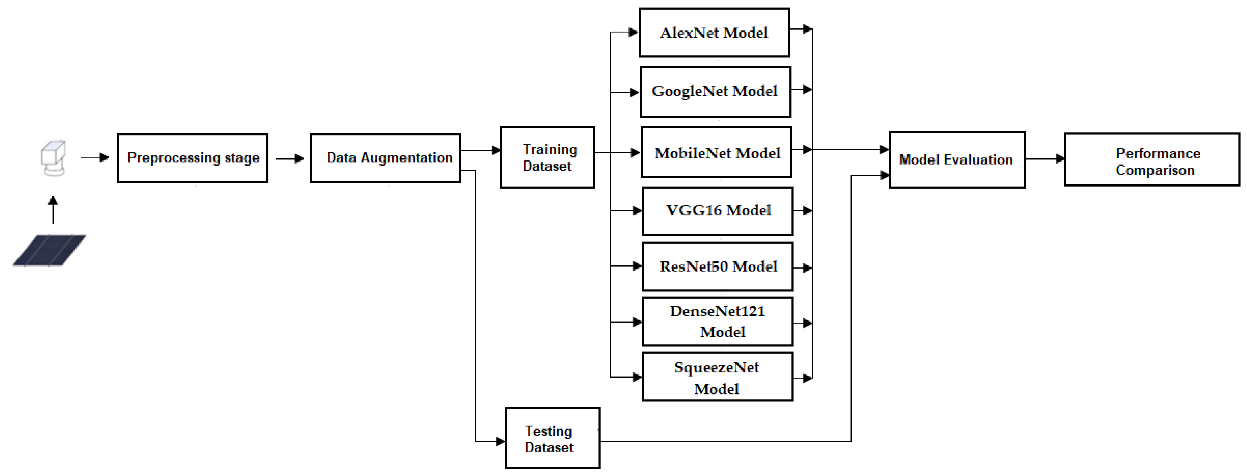
2. Materials and Methods

In this study, fast and high-accuracy detection of invisible cracks and fractures in solar panel cells was carried out. For this purpose, electroluminescence and deep learning were worked together. Monocrystalline and polycrystalline solar panel cell images were taken with electroluminescence. A data multiplication process was performed to distribute the dataset equally. Then, a classification process was performed in deep learning. AlexNet, GoogleNet, MobileNet, VGG16, ResNet50, DenseNet121 and SqueezeNet architectures were used to obtain the highest accuracy. The same dataset was used in deep learning architectures. The dataset was resized for each architecture. The highest accuracy rate was obtained in the classification of monocrystalline and polycrystalline solar panel cells. Figure 1 shows the general working principle of the system.

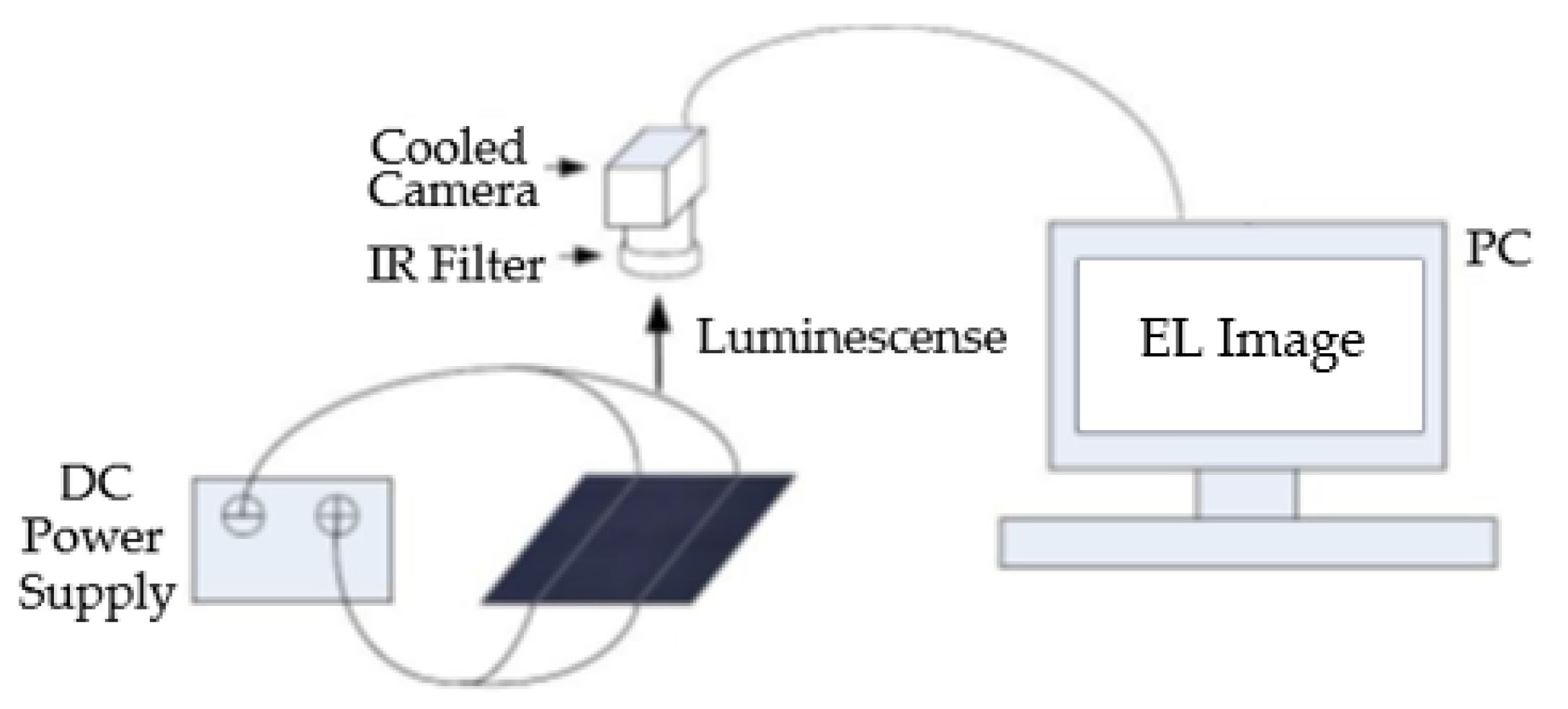
2.1. Electroluminescence

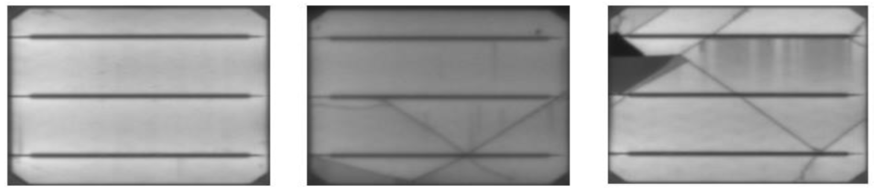
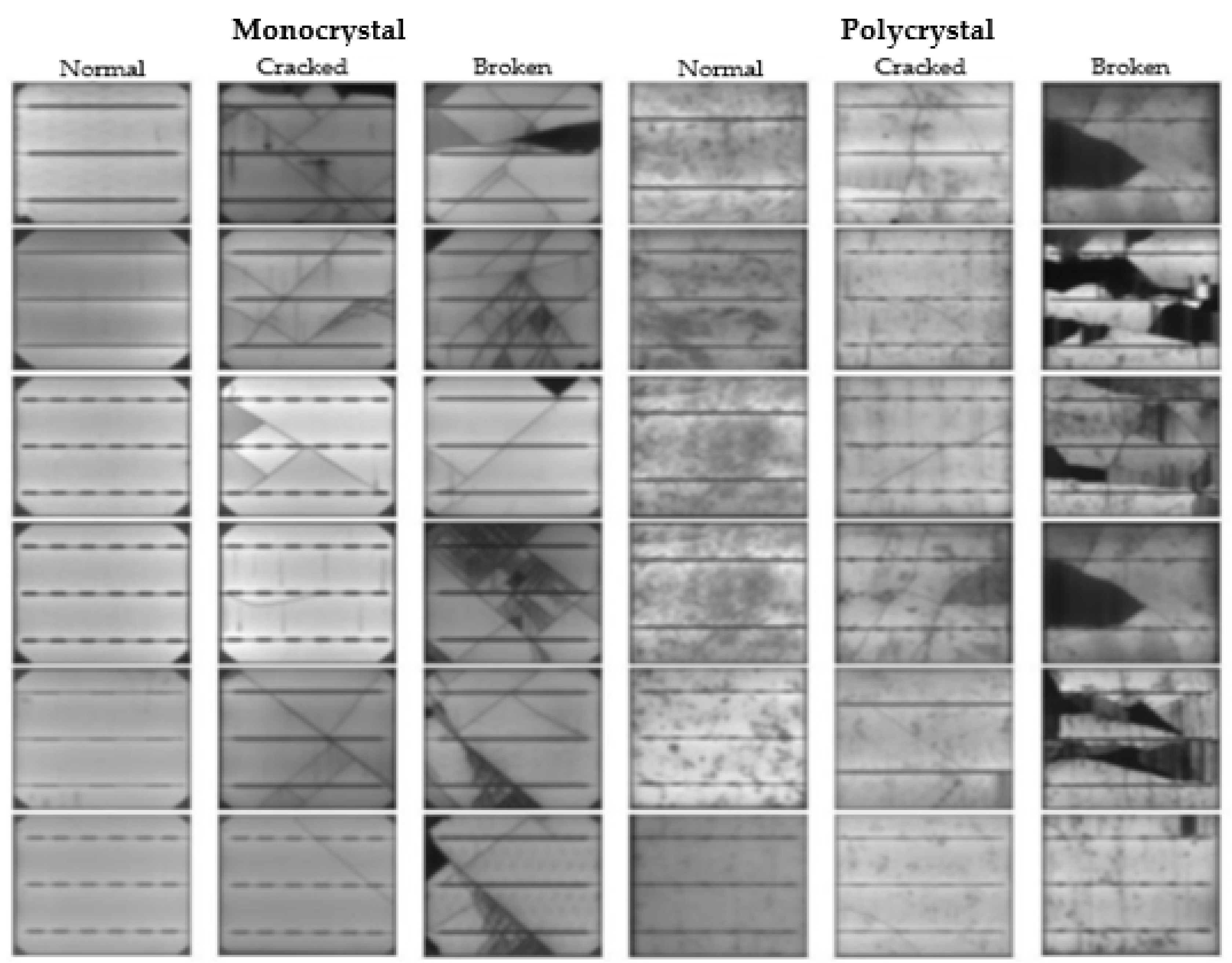
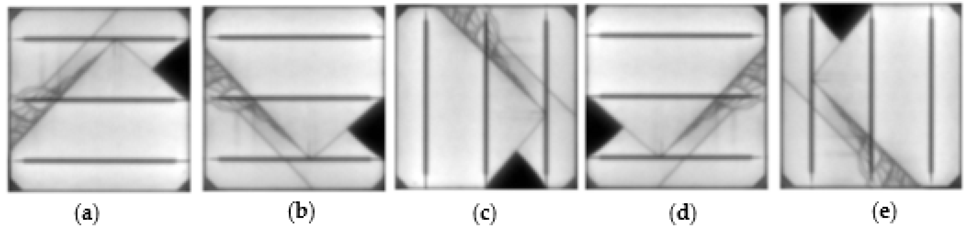
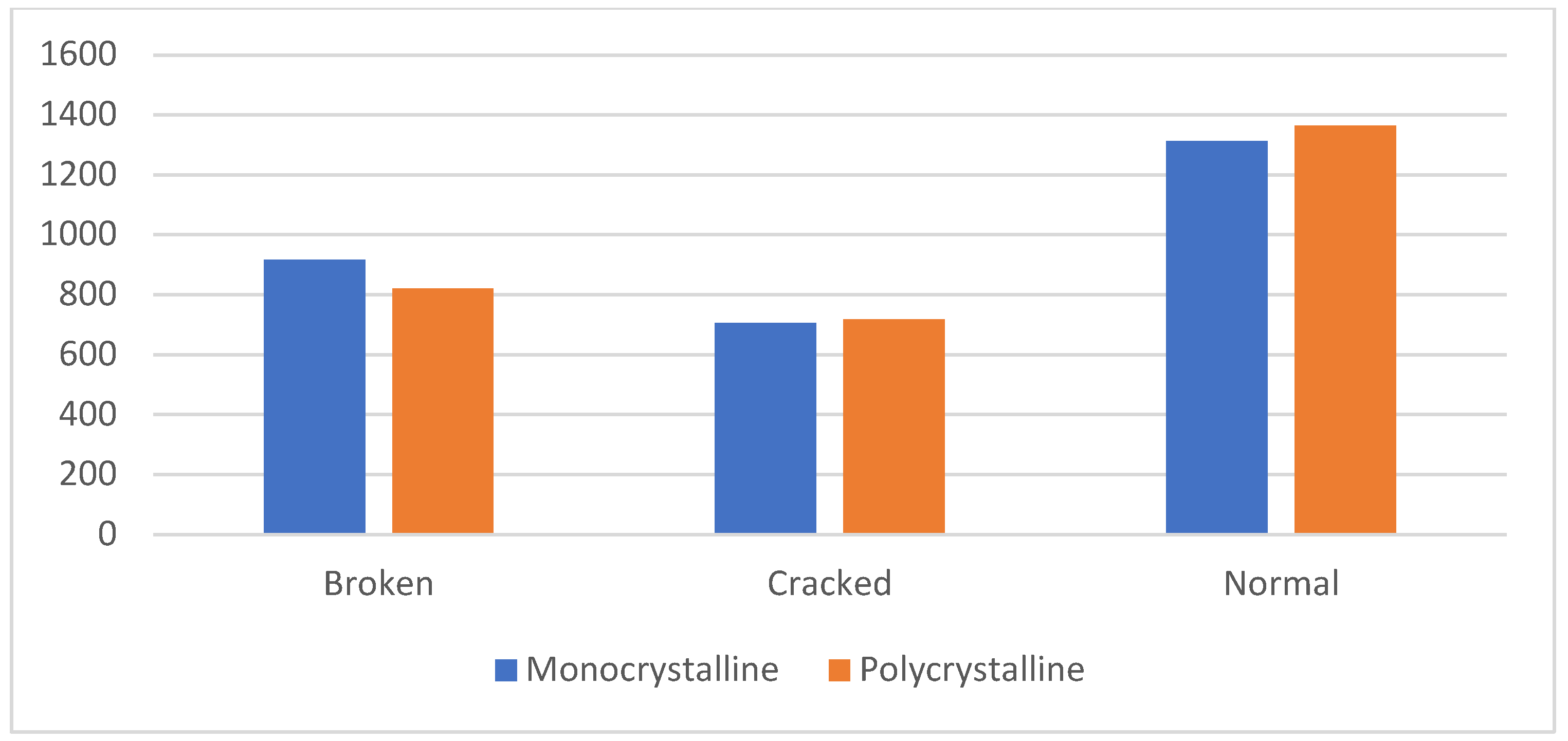
Electroluminescence imaging is a technique used for the visual inspection of photovoltaic modules. It allows for capturing high-resolution images of photovoltaic modules and identifying defects. The working logic of electroluminescence imaging is shown in Figure 2. The image of a solar panel is taken in the dark with a special camera with an infrared filter and transferred to a computer environment. The electroluminescence images formed are evaluated according to their conditions and it is determined whether they are damaged or not [22,23,24].

Figure 3 shows intact, cracked and broken solar cells obtained after electroluminescence testing. It is very difficult to determine the robustness of solar cells without any external equipment. Therefore, by finding and replacing defects in solar cells with this imaging, the efficiency obtained from solar panels increases. This will prevent bigger problems that may occur in the future [25].

2.2. Dataset

In this study, a publicly available solar panel dataset obtained from high-resolution EL images of monocrystalline and polycrystalline PV panels was used [8,25]. This dataset includes 51 different PV panels. The dataset consists of 5836 solar panel cells with a resolution of 300 × 300 pixels. A total of 22 of the solar panel cells in the dataset are monocrystalline and 29 are polycrystalline. A total of 1736 images represent the fracture class. In the dataset, 1424 images are in the crack class and the remaining 2676 images are intact cell images.

The dataset was obtained by collection from different angles in a test laboratory environment and under controlled conditions. Thus, the factors that would have negatively affected the image quality were minimized. Some samples were edited with preprocessing steps such as cropping, scaling and rotation. Considering that PV panels emit only one light when shooting in a dark room, illuminating the images homogeneously was considered. The dataset includes cells with micro-cracks and electrically separated and deteriorated parts, short-circuited cells, open-circuit interconnects and soldering errors. Thus, common faults that negatively affect the efficiency, reliability and durability of PV panels are represented [8]. Figure 4 shows different sample images in the dataset.

2.3. Data Replication

The number of samples in a dataset affects the performance of deep learning models. Generally, training ESAs with a limited number of data causes over-learning and the generalizability of the trained network is not high. However, increasing the number of samples in the dataset in terms of quantity, quality and diversity can increase the training performance of the developed network. Data augmentation is one of the popular methods used in classification problems and in cases where there is not enough data. Synthetic data production is performed with data augmentation. Data augmentation provides better classification performance by preventing over-learning caused by limited samples. Thus, the irregularity between the class distributions is minimized and the same number of clustering is performed for all classes.

The PV dataset used in this study includes a total of 5836 EL images belonging to the healthy, cracked and broken classes. However, there are 2676 images for the healthy class, which is less than half of the functional class. In addition, the classification of monocrystalline and polycrystalline solar panel cells was performed in separate halves in this study. For this reason, the dataset was divided into two. The size of the two datasets was the same. Thus, the error rate was minimized during the comparison. In this case, the distribution of the classes was irregular and it was necessary to increase the samples for the training performance of the proposed network. Inversion and rotation techniques were applied in data augmentation to preserve the general structure represented by the dataset. In the inversion process, the elements in the columns and rows were reversed. In the rotation process, the images were rotated around their central point by 90°, 180° and 270° counterclockwise. Thus, five different synthetic images were obtained for each class example. In Figure 5, synthetic images obtained as a result of data augmentation for a sample image selected from the defective class are given. Figure 6 shows the numbers of normal, cracked and broken solar panel cells used in the dataset.

2.4. Deep Learning

Deep learning is a type of machine learning that exhibits behaviors similar to human learning and thinking abilities. While in machine learning models, the features of each class in the training data are extracted manually or with special methods depending on the scenario, in deep learning, these features are extracted and learned automatically. Therefore, the main purpose of deep learning algorithms is to automate the extraction of representations from data.

People and computers can transfer the same or similar features from the same images in different ways. For example; while people can verbally express the numbers, colors, shapes and positions of objects in any image, computers express each object in the same image or images as a matrix of numbers.

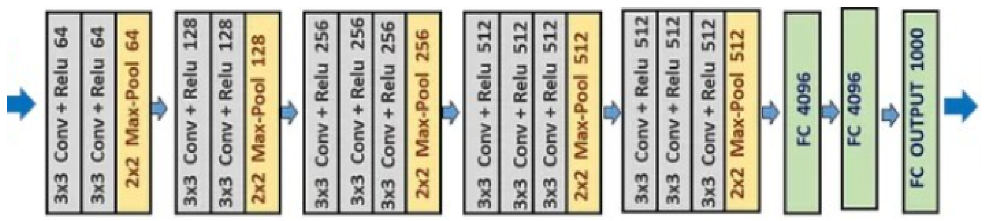
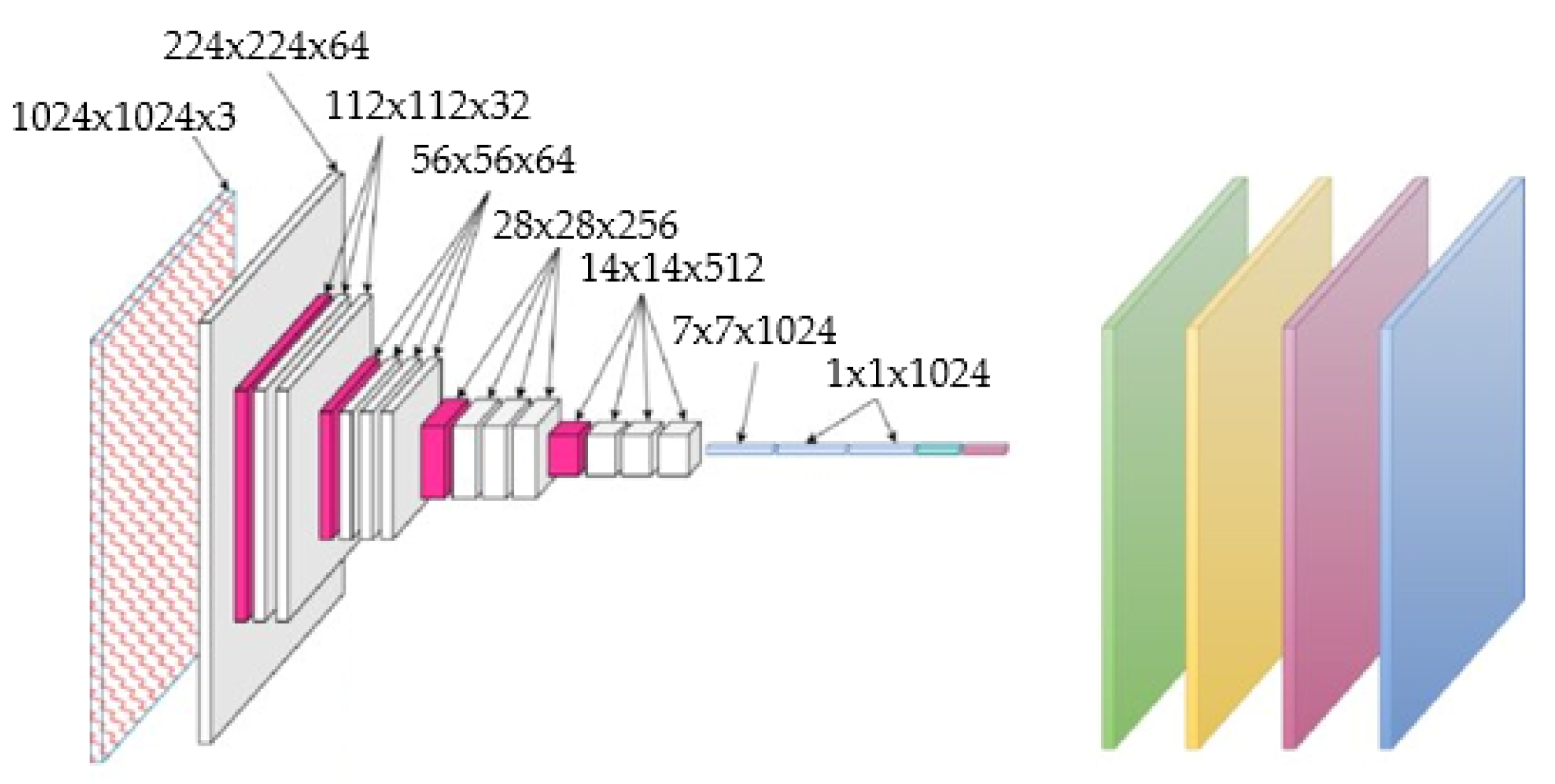
2.4.1. VGG16 Architecture

VGG16, a variant of VGGNet, can be described as a simple and widely used architecture for ImageNet. The model’s architecture is seen in Figure 7; the first and second layers consist of a 64-feature kernel filter with a filter size of 3 × 3 and passed to the max pooling layer in the next two layers. In the third and fourth convolutional layers, there is a 128-feature kernel filter with a filter size of 3 × 3 and passed to the next 2-step max pooling layer. The fifth, sixth and seventh layers consist of a 256-feature kernel filter with a filter size of 3 × 3 and passed to the next 2-step max pooling layer. Between the eighth and thirteenth layers, a 512-feature kernel filter with a filter size of 3 × 3 is created and then the max pooling layer is continued with a 1-step max pooling layer. Layers 14 and 15 are fully connected layers consisting of 4096 units, and finally, layer 16 consists of a SoftMax output layer consisting of 1000 units. Figure 7 shows the VGG16’s architecture.

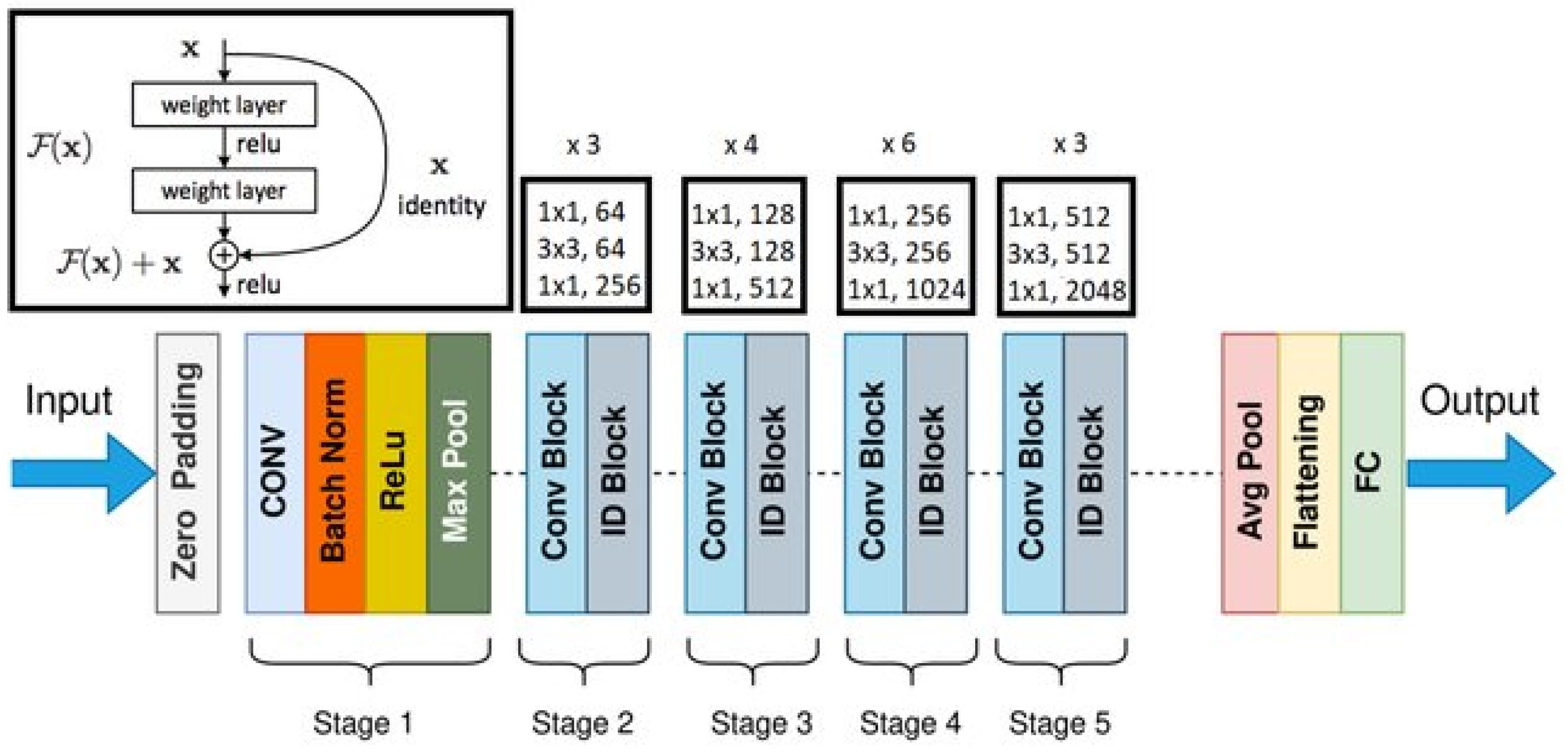
2.4.2. ResNet50 Architecture

ResNet, short for Residual Network, is a widely used neural network architecture that serves as a backbone for numerous computer vision applications. One popular variant, ResNet50, comprises 50 layers, allowing for the training of very deep networks, even exceeding 150 layers. The major innovation of ResNet is its ability to train such deep models effectively.

ResNet50’s architecture consists of four main stages, with an input size of 224 × 224 × 3. The network begins with an initial 7 × 7 convolution followed by a 3 × 3 max pooling layer. Stage 1 features three residual blocks, each containing three layers. These layers use kernels sized 64, 64 and 128, respectively. Identity connections are represented by curved arrows, while dashed arrows indicate steps where the input size is halved, and the number of channels is doubled due to convolutional operations. Figure 8 illustrates ResNet50’s architecture.

2.4.3. MobileNet Architecture

MobileNet, introduced by Google’s team in 2017, is a lightweight convolutional neural network designed specifically for mobile and embedded devices. A key feature of MobileNet is its use of depthwise separable convolution, which breaks down the traditional convolutional process into two distinct steps: depthwise convolution and pointwise convolution.

MobileNet’s design includes two hyperparameters that enable the adjustment of the balance between efficiency and accuracy. The architecture relies on depthwise separable convolutions composed of depth and point convolutional layers. The depth convolution filters the input without altering its structure, while the pointwise convolution combines these filtered outputs to create new features. The combination of these layers forms a depthwise separable convolution. Each convolutional step in MobileNet incorporates batch normalization and a modified ReLU activation function. Figure 9 illustrates MobileNet’s architecture.

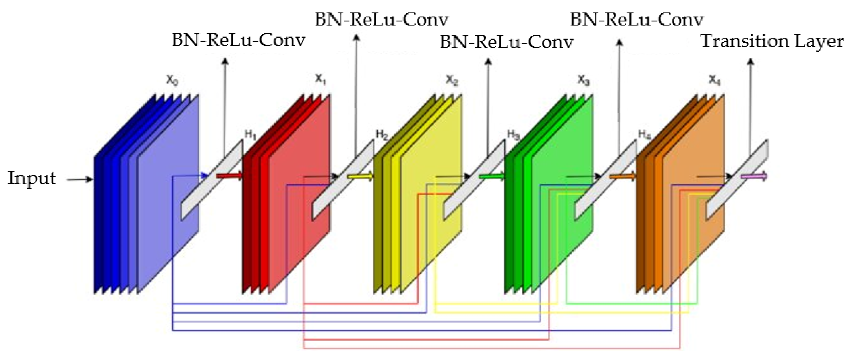
2.4.4. DenseNet121 Architecture

As the number of layers in a convolutional neural network (CNN) increase, the issue known as the “vanishing gradient” problem can occur. This problem means that as the pathway between the input and output layers becomes longer, the signal can weaken, leading to loss of information and reduced training efficiency. DenseNets address this issue by altering the traditional CNN architecture and streamlining the connections between layers. An example of the DenseNet121 architecture can be seen in Figure 10.

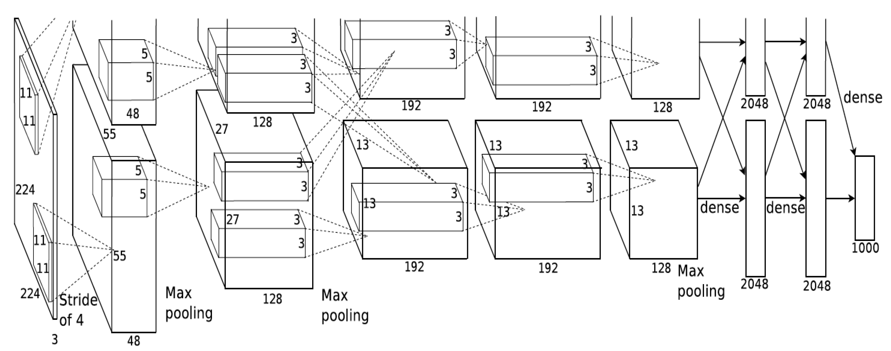
2.4.5. AlexNet Architecture

AlexNet is a deep learning algorithm developed by Alex Krizhevsky, Ilya Sutskever and Geoffrey Hinton. This deep convolutional neural network is composed of 25 layers, including five convolutional layers, three max-pooling layers, two dropout layers, three fully connected layers, seven ReLU activation layers, two normalization layers, a softmax layer, as well as input and output layers. The input image size for the network is 227 × 227 × 3. The architecture of AlexNet is illustrated in Figure 11.

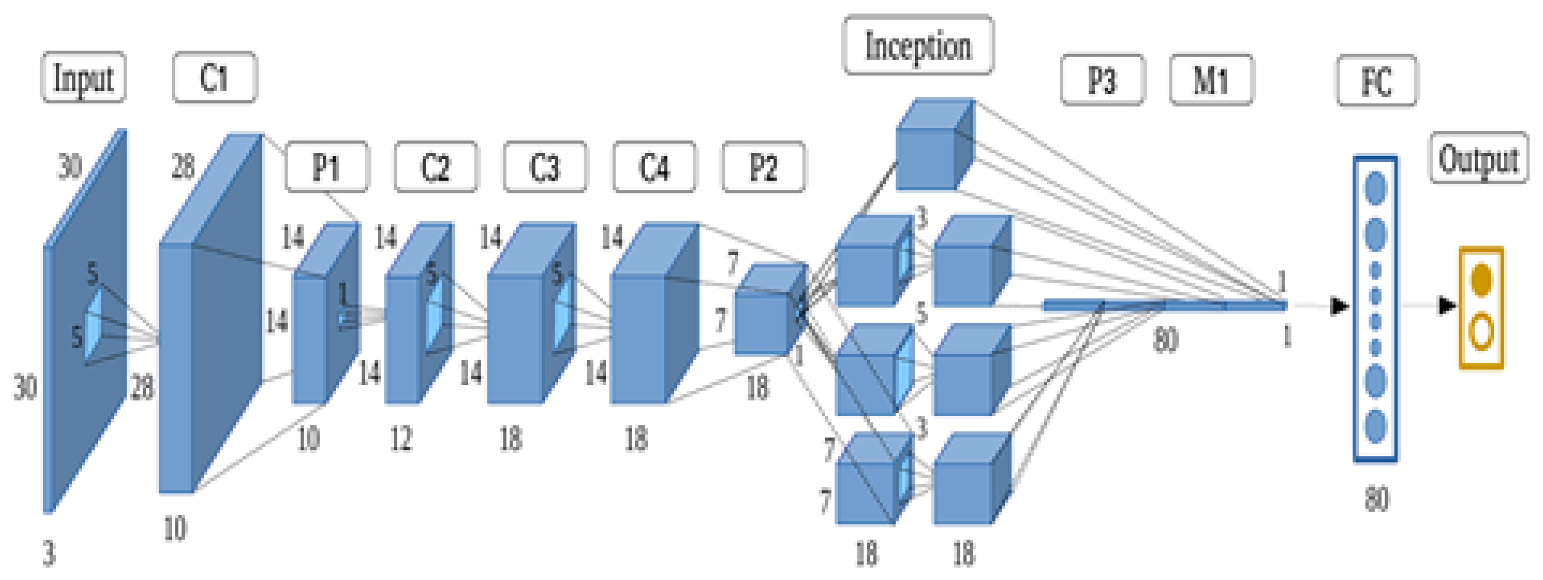
2.4.6. GoogleNet Architecture

The GoogleNet algorithm was the winner of the ILSVRC competition held in 2014. The structure of the algorithm is complex. It has a high accuracy rate with a very low error rate. The GoogleNet algorithm is a deep learning algorithm that has achieved an accuracy rate of 93% on the ImageNet database. It contains 12 times more parameters than AlexNet. It has a depth of 27 layers, including pooling layers. Its architectural structure consists of approximately 100 layers. The algorithm has a total of 144 layers, including convolutional, maxpooling, softmax, fully connected, ReLU, input and output layers. The image in the input layer is 224 × 224 × 3. Google Net’s architecture is shown in Figure 12.

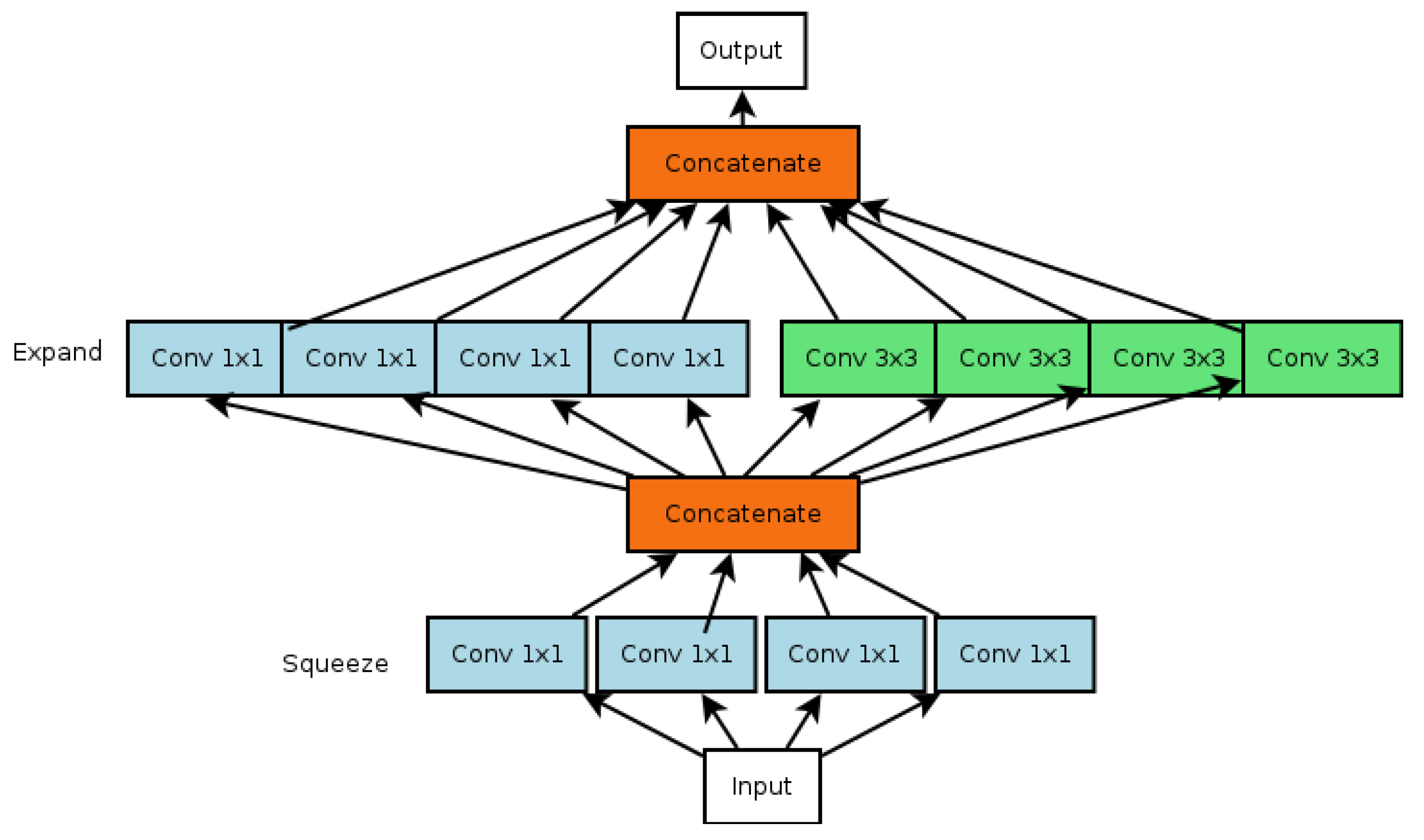
2.4.7. SqueezeNet Architecture

Another popular architecture used in the convolutional neural network model is the SqueezeNet architecture. The aim of this architecture is to create a neural network with fewer parameters. It provides AlexNet-level accuracy with 50 times fewer parameters. The advantage of the SqueezeNet architecture is that it reduces the workload on the neural network thanks to more efficient distributed layers and thus works faster. The SqueezeNet architecture was first demonstrated in a study conducted by Iandola et al. The algorithm has an input dog image, two convolutional layers in each algorithm, conv1 and conv10, a total of eight firing modules, fire2, fire3, fire4, fire5, fire6, fire7, fire8 and fire9, and finally a smoothing layer such as softmax. There are pooling layers in the first convolutional layer, the fourth firing module, the eighth firing module and the 10th convolutional layer. The layers and connections of the SqueezeNet architecture are shown in Figure 13.

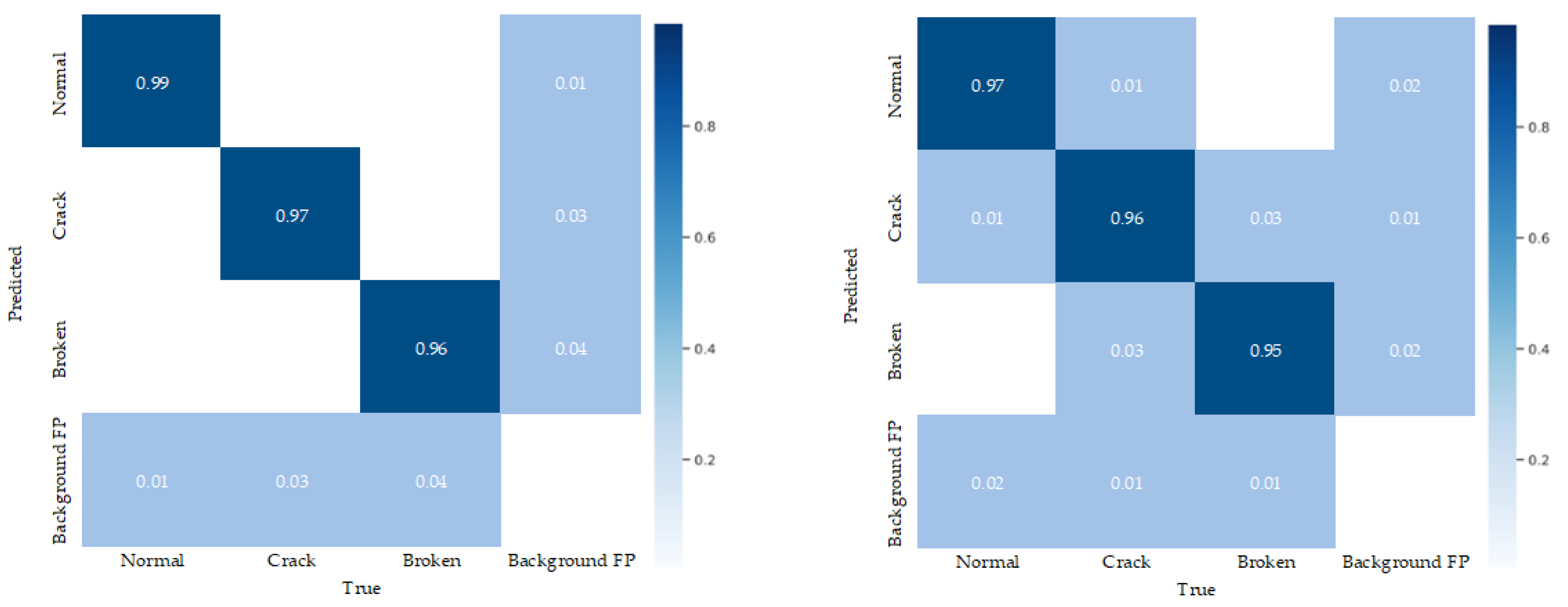
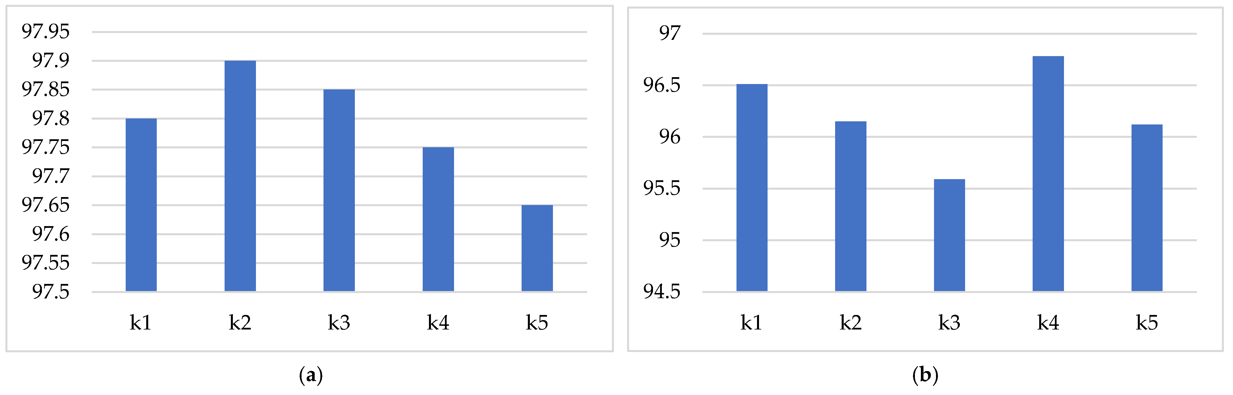
3. Result and Discussion

In this study, monocrystalline and polycrystalline solar panels were used. Three classifications were made for the solar panels: normal, cracked and broken. Each solar panel is included in the dataset in equal numbers. The classification process was performed in seven different architectures in deep learning. The same dataset was used in each architecture. The error rate was minimized when comparing the deep learning architecture results. The image dimensions that make up the dataset were changed in accordance with the architectures.

Table 1. Results of running the monocrystalline and polycrystalline solar panel dataset on seven different architectures.

Class	Types of Solar Panels	Accuracy	Precision	Recall	F1-Score
AlexNet	Monocrystalline	86.89	81.05	86.53	82.99
	Polycrystalline	85.26	79.96	84.16	80.69
GoogleNet	Monocrystalline	87.25	82.13	87.02	84.08
	Polycrystalline	86.78	81.01	85.96	83.13
MobileNet	Monocrystalline	88.01	84.07	87.25	84.93
	Polycrystalline	87.23	82.05	85.78	83.36
VGG16	Monocrystalline	91.26	86.48	89.89	86.15
	Polycrystalline	90.01	85.29	87.47	85.19
ResNet50	Monocrystalline	93.48	87.63	90.37	87.81
	Polycrystalline	91.25	87.08	89.45	86.89
DenseNet121	Monocrystalline	96.17	89.42	91.48	91.89
	Polycrystalline	96.01	89.27	90.82	90.12
SqueezeNet	Monocrystalline	97.82	91.75	95.81	95.39
	Polycrystalline	96.42	90.82	94.72	94.57

shows the results of running the monocrystalline and polycrystalline solar panel dataset on seven different architectures.

As a result of this study, the lowest accuracy rate in monocrystalline solar panel cells was 86.89% in the AlexNet architecture. The highest accuracy rate was 97.82% in the SqueezeNet architecture. Although the architectures used the same dataset, the accuracy rates were different due to the changes in their internal structures.

In this study, a data augmentation process was applied. Thanks to this process, a high accuracy rate of 97.82% was achieved. Figure 14 shows the accuracy rates of seven different architectures before applying the data augmentation process.

Before applying data augmentation, the highest accuracy rate was 95.87% with SqueezeNet. The lowest accuracy rate was 84.09% with AlexNet. Data augmentation increased the accuracy rates of seven different deep learning models. These increase rates ranged from 4.56% to 1.17%.

The highest classification of polycrystalline solar panels was achieved with 96.42% in SqueezeNet architecture. The accuracy rate of the polycrystalline solar panel cells was 1.30% lower. The main reason for this is due to the materials used during production. There is a homogeneous distribution in monocrystalline solar panel cells. This homogeneous distribution provides a clearer and clearer image in the images. Cracks and fractures appear much clearer in these images. There is a heterogeneous situation in the production of polycrystalline solar panel cells. In this way, a clear image cannot be obtained from polycrystalline solar panel cells. This makes it difficult to see cracks and fractures. For this reason, the classification rates in polycrystalline solar panel cells were lower. In this study, three classifications were made as normal, cracked and broken. These three classifications had different accuracy rates. The average accuracy rates are taken into account in Table 1. The results of the SqueezeNet architecture, which gave the highest accuracy rate, are shown in detail in

Table 2. Results of SqueezeNet architecture.

Class	Types of Solar Panels	Accuracy	Precision	Recall	F1-Score
Normal	Monocrystalline	98.99	93.25	97.49	96.53
	Polycrystalline	97.26	92.36	95.54	95.63
Cracked	Monocrystalline	97.47	90.15	95.70	95.02
	Polycrystalline	96.51	90.95	94.96	94.92
Broken	Monocrystalline	96.99	91.60	94.24	94.61
	Polycrystalline	95.26	89.15	93.66	92.16
Average	Monocrystalline	97.82	91.75	95.81	95.39
	Polycrystalline	96.42	90.82	94.72	94.57

.

In monocrystalline solar panel cells, normal classification had the highest classification result with 98.99%. The solar panel cell fracture and crack classification accuracy results were 97.47% and 96.99%, respectively. In polycrystalline solar panel cells, the highest result was 97.26% in normal classification and the lowest was 95.26% in fracture classification. Figure 15 shows confusion matrices of the SqueezeNet architecture for the monocrystalline and polycrystalline solar panel cells.

Confusion matrix application was carried out to evaluate the performance of this study. The performance of the classification algorithm was visualized with confusion matrices. For the confusion matrices, 1500 images were used for detection. Figure 16 shows the confusion matrix results.

A total of 500 test operations were carried out for each class of monocrystalline and polycrystalline solar panel cells. As a result of the test operations, an average accuracy of 97.53% was obtained for monocrystalline solar panel cells and 95.46% for polycrystalline solar panel cells. The values obtained as a result of the test operations had a very small difference between normal values.

The K-Fold Cross Validation method divides a dataset into “k” equal parts and creates validation data for each part one by one. Thus, each data point is used as a validation datum at least once. In this way, the overall performance of a model is evaluated more accurately. There were 9000 samples in the dataset of this study. Here, the number k was determined as 5. In other words, the dataset was divided into 5. There were 1800 samples in each dataset. They were distributed in the same proportions as in the general dataset. Figure 17 shows the results of the K-Fold Cross Validation method.

Using the K-Fold Cross Validation method, the average accuracy rate was 97.379% for the monocrystalline solar panel cells and 96.23% for the polycrystalline solar panel cells. With this result, the two results that were checked as the general result of the system were very close to each other. Therefore, it is understood that the overall performance of the model was good.

When the literature was examined, it was seen that many studies had been conducted on this topic. Different architectures were used in these studies.

Table 3. Literature studies.

Authors	Architecture	Accuracy %
Kasemann et al. [26]	CNN	93.02
Buerhop-Lutz et al. [2]	VGG19	88.42
Ge et al. [27]	Fuzzy-CNN	88.35
Deitsch et al. [3]	SeF-HRNet	94.90
Wang et al. [28]	ResNet152	92.13
Açikgöz et al. [29]	Res-INC-V3-SPP	93.59
Munawer et al. [30]	CNN-ILD	95.80
Xie et al. [31]	ConvNext-CNFP	96.36
Krovin et al. [32]	CNN	85.20
Tang et al. [33]	CNN	83.00
Et-talebi et al. [34]	CNN + SWM	90.57
Karimi et al. [35]	YOLO	78
Chen et al. [36]	VGG16	82
Zhang et al. [37]	Faster R-CNN	91.3
Zhao et al. [38]	Mask R-CNN	70.2
Firesi et al. [39]	ResNet50	95.4
Akram et al. [40]	GCAM- EfficientNet	93.59
Xialog et al. [41]	CNN	88.12
Wang et al. [42]	CNN	92.02
This study	AlexNet, GoogleNet, MobileNet, VGG16, ResNet50, DenseNet121, SqueezeNet	97.82

shows a comparison of these literature studies.

There are different studies in the literature. Different machine learning and deep learning architectures were used in these studies, and very different accuracy results were obtained. When the accuracy results were compared, the highest accuracy rate was achieved from the present study. The most important reasons for this are the dataset prepared for this study and the different deep learning architectures employed; an original and new dataset was prepared for this study in which separate studies were conducted for monocrystalline and polycrystalline solar panel cells. The dataset was classified into three categories: intact, broken and cracked. The samples used in this classification were obtained from a real environment. By making changes to the dataset, both the dataset was increased. At the same time, errors that may have occurred later were avoided and the error rate was reduced.

Seven different deep learning architectures were used in this study. In this way, the highest accuracy rate was achieved. Deep learning architectures offer different accuracy rates in different studies. For this reason, the highest accuracy rate of 97.82% was obtained with the most commonly used deep learning architectures.

A high level of accuracy was achieved in this study. However, errors that may occur during the various methods used in this study may have caused a decrease in accuracy rates. The most important of these errors are errors that may occur with the camera. Camera shaking and inversion and rotation of solar panel cells are the most common errors. Changes were made to the dataset to prevent camera and solar cell rotation errors. Errors that may have occurred due to the camera could be minimized by making changes to the photographs in the dataset, such as adjusting the gray tone, adding color tone, adding blur, adding noise, cropping and changing the image brightness.

4. Conclusions

In this study, the detection of fractures and cracks in monocrystalline and polycrystalline solar panel cells was carried out. With this study, damages occurring in solar panel cells were detected quickly and with high accuracy. An original and new dataset was prepared for this study. Electroluminescence images of monocrystalline and polycrystalline solar panel cells were taken using a dataset. The dataset was used in seven different AlexNet, GoogleNet, MobileNet, VGG16, ResNet50, DenseNet121 and SqueezeNet architectures in deep learning. Monocrystalline and polycrystalline solar panel cells were classified separately. Three determinations were made for classification: intact, cracked or broken. Monocrystalline and polycrystalline solar panel cells achieved the highest results of 97.89% and 96.29% accuracy, respectively, using the SqueezeNet architecture. To maintain accuracy during this study, 500 test operations were performed for each class for monocrystalline and polycrystalline solar panel cells. As a result of the test operations, 97.53% and 95.46% were achieved in monocrystalline and polycrystalline solar panel cells, respectively. The dataset was divided into five equal parts with the K-Fold Cross Validation method. Then, a reclassification process was performed on each part. After the K-Fold Cross Validation method, 97.39% accuracy was achieved in the monocrystal-line solar panel cells and 96.23% in the polycrystalline solar panel cells. The classification, test process and K-Fold Cross Validation method results were very close to each other. This shows the accuracy of this study.

In future studies, increasing the datasets used will affect accuracy rates. Especially with the use of different deep learning methods, more successful classification will occur.

References

1. Demirci, M.Y.; Beşli, N.; Gümüşçü, A. Efficient deep feature extraction and classification for identifying defective photovoltaic module cells in Electroluminescence images. Expert. Syst. Appl. 2021, 175, 114810. [Google Scholar] [CrossRef]
2. Buerhop-Lutz, C.; Deitsch, S.; Maier, A.; Gallwitz, F.; Berger, S.; Doll, B.; Brabec, C.J. A benchmark for visual identification of defective solar cells in electroluminescence imagery. In Proceedings of the 35th European PV Solar Energy Conference and Exhibition, Brussels, Belgium, 24–28 September 2018. [Google Scholar]
3. Deitsch, S.; Christlein, V.; Berger, S.; Buerhop-Lutz, C.; Maier, A.; Gallwitz, F.; Riess, C. Automatic classification of defective photovoltaic module cells in electroluminescence images. Sol. Energy 2019, 185, 455–468. [Google Scholar] [CrossRef]
4. Chen, H.; Zhao, H.; Han, D.; Liu, K. Accurate and robust crack detection using steerable evidence filtering in electroluminescence images of solar cells. Opt. Lasers Eng. 2019, 118, 22–33. [Google Scholar] [CrossRef]
5. Ali, M.U.; Khan, H.F.; Masud, M.; Kallu, K.D.; Zafar, A. A machine learning framework to identify the hotspot in photovoltaic module using infrared thermography. Sol. Energy 2020, 208, 643–651. [Google Scholar] [CrossRef]
6. Pratt, L.; Govender, D.; Klein, R. Defect detection and quantification in electroluminescence images of solar PV modules using U-net semantic segmentation. Renew. Energy 2021, 178, 1211–1222. [Google Scholar] [CrossRef]
7. Naveen Venkatesh, S.; Sugumaran, V. Machine vision based fault diagnosis of photovoltaic modules using lazy learning approach. Meas. J. Int. Meas. Confed. 2022, 191, 110786. [Google Scholar] [CrossRef]
8. Moradi Sizkouhi, A.; Aghaei, M.; Esmailifar, S.M. A deep convolutional encoder-decoder architecture for autonomous fault detection of PV plants using multi-copters. Sol. Energy 2021, 223, 217–228. [Google Scholar] [CrossRef]
9. Chindarkkar, A.; Priyadarshi, S.; Shiradkar, N.S.; Kottantharayil, A.; Velmurugan, R. Deep Learning Based Detection of Cracks in Electroluminescence Images of Fielded PV modules. In Proceedings of the 2020 47th IEEE Photovoltaic Specialists Conference, Calgary, AB, Canada, 15 June–21 August 2020; pp. 1612–1616. [Google Scholar] [CrossRef]
10. Haidari, P.; Hajiahmad, A.; Jafari, A.; Nasiri, A. Deep learning-based model for fault classification in solar modules using infrared images. Sustain. Energy Technol. Assess. 2022, 52, 102110. [Google Scholar] [CrossRef]
11. Rico Espinosa, A.; Bressan, M.; Giraldo, L.F. Failure signature classification in solar photovoltaic plants using RGB images and convolutional neural networks. Renew. Energy 2020, 162, 249–256. [Google Scholar] [CrossRef]
12. Su, B.; Chen, H.; Liu, K.; Liu, W. RCAG-Net: Residual Channelwise Attention Gate Network for Hot Spot Defect Detection of Photovoltaic Farms. IEEE Trans. Instrum. Meas. 2021, 70, 3510514. [Google Scholar] [CrossRef]
13. Fuyuki, T.; Kondo, H.; Kaji, Y.; Yamazaki, T.; Takahashi, Y.; Uraoka, Y. One shot mapping of minority carrier diffusion length in polycrystalline silicon solar cells using electroluminescence. Sol. Energy 2005, 1343–1345. [Google Scholar] [CrossRef]
14. Breitenstein, O.; Bauer, J.; Bothe, K.; Hinken, D.; Müller, J.; Kwapil, W.; Schubert, M.C. Can Luminescence Imaging Replace Lock-In Thermography on Solar Cells and Wafers? In Proceedings of the 37th IEEE Photovoltaic Specialists Conference, Seattle, WA, USA, 19–24 June 2011; pp. 159–167. [Google Scholar] [CrossRef]
15. Qian, X.; Li, J.; Cao, J.; Wu, Y.; Wang, W. Micro-cracks detection of solar cells surface via combining short-term and long-term deep features. Neural Netw. 2020, 127, 132–140. [Google Scholar] [CrossRef]
16. Chen, H.; Pang, Y.; Hu, Q.; Liu, K. Solar cell surface defect inspection based on multispectral convolutional neural network. J. Intell. Manuf. 2020, 31, 453–468. [Google Scholar] [CrossRef]
17. Gallardo-Saavedra, S.; Hernández-Callejo, L.; del Carmen Alonso-García, M.; Santos, J.D.; Morales-Aragonés, J.I.; Alonso-Gómez, V.; Moretón-Fernández, Á.; González-Rebollo, M.Á.; Martínez-Sacristán, O. Nondestructive characterization of solar PV cells defects by means of electroluminescence, infrared thermography, I–V curves and visual tests: Experimental study and comparison. Energy 2020, 205, 117930. [Google Scholar] [CrossRef]
18. Mathias, N.; Shaikh, F.; Thakur, C.; Shetty, S.; Dumane, P.; Chavan, D. Detection of Micro-Cracks in Electroluminescence Images of Photovoltaic Modules. In Proceedings of the 3rd International Conference on Advances in Science & Technology (ICAST), Bahir Dar, Ethiopia, 8–10 May 2020; pp. 342–347. [Google Scholar] [CrossRef]
19. Fan, T.; Sun, T.; Xie, X.; Liu, H.; Na, Z. Automatic Micro-Crack Detection of Polycrystalline Solar Cells in Industrial Scene. IEEE Access 2022, 10, 16269–16282. [Google Scholar] [CrossRef]
20. Rahman, M.R.; Tabassum, S.; Haque, E.; Nishat, M.M.; Faisal, F.; Hossain, E. CNN-based Deep Learning Approach for Micro-crack Detection of Solar Panels. In Proceedings of the 2021 3rd International Conference on Sustainable Technologies for Industry 4.0 (STI), Dhaka, Bangladesh, 18–19 December 2021; pp. 1–6. [Google Scholar] [CrossRef]
21. Grunow, P.; Clemens, P.; Hoffmann, V.; Litzenburger, B.; Podlowski, L. Influence of Micro Cracks in Multi-Crystalline Silicon Solar Cells on the Reliability of Pv Modules. In Proceedings of the 20th European Photovoltaic Solar Energy Conference, Barcelona, Spain, 6–10 June 2005; pp. 2380–2383. [Google Scholar]
22. Köntges, M.; Kurtz, S.; Packard, C.; Jahn, U.; Berger, K.A.; Kato, K.; Friesen, T. Review of Failures of Photovoltaic Modules; IEA—International Energy Agency: Paris, France, 2014. [Google Scholar]
23. Bothe, K.; Pohl, P.; Schmidt, J.; Weber, T.; Altermatt, P.; Fischer, B.; Brendel, R. Electroluminescence Imaging as an In-Line Characterisation Tool for Solar Cell Production. In Proceedings of the 21st European Photovoltaik Solae Energy Conference, Dresden, Germany, 4–8 September 2006; pp. 597–600. [Google Scholar]
24. Tsai, D.M.; Wu, S.C.; Li, W.C. Defect detection of solar cells in electroluminescence images using Fourier image reconstruction. Sol. Energy Mater. Sol. Cells 2012, 99, 250–262. [Google Scholar] [CrossRef]
25. Denio, H. Aerial solar thermography and condition monitoring of photovoltaic systems. In Proceedings of the 2012 38th IEEE Photovoltaic Specialists Conference, Austin, TX, USA, 3–8 June 2012. [Google Scholar]
26. Kasemann, M.; Kwapil, W.; Walter, B.; Giesecke, J.; Michl, B.; The, M.; Glunz, S.W. Progress in silicon solar cell characterization with infrared imaging methods. In Proceedings of the 23rd European Photovoltaic Solar Energy Conference, Valencia, Spain, 1–5 September 2008; pp. 965–973. [Google Scholar]
27. Ge, C.; Liu, Z.; Fang, L.; Ling, H.; Zhang, A.; Yin, C. A hybrid fuzzy convolutional neural network based mechanism for photovoltaic cell defect detection with electroluminescence images. IEEE Trans. Parallel Distrib. Syst. 2021, 32, 1653–1664. [Google Scholar] [CrossRef]
28. Wang, J.; Bi, L.; Sun, P.; Jiao, X.; Ma, X.; Lei, X.; Luo, Y. Deep-learning-based automatic detection of photovoltaic cell defects in electroluminescence images. Sensors 2023, 23, 297. [Google Scholar] [CrossRef]
29. Acikgoz, H.; Korkmaz, D.; Budak, U. Photovoltaic cell defect classification based on integration of residual-inception network and spatial pyramid pooling in electroluminescence images. Expert Syst. Appl. 2023, 229, 120546. [Google Scholar] [CrossRef]
30. Munawer Al-Otum, H. Deep learning-based automated defect classification in electroluminescence images of solar panels. Adv. Eng. Inform. 2023, 58, 102147. [Google Scholar] [CrossRef]
31. Xie, X.; Lai, G.; You, M.; Liang, J.; Leng, B. Effective transfer learning of defect detection for photovoltaic module cells in electroluminescence images. Sol. Energy 2023, 250, 312–323. [Google Scholar] [CrossRef]
32. Korovin, A.; Vasilev, A.; Egorov, F.; Saykin, D.; Terukov, E.; Shakhray, I.; Zhukov, L.; Budennyy, S. Anomaly detection in electroluminescence images of heterojunction solar cells. Sol. Energy 2023, 259, 130–136. [Google Scholar] [CrossRef]
33. Tang, W.; Yang, Q.; Xiong, K.; Yan, W. Deep learning based automatic defect identification of photovoltaic module using electroluminescence images. Sol. Energy 2020, 201, 453–460. [Google Scholar] [CrossRef]
34. Et-taleby, A.; Chaibi, Y.; Allouhi, A.; Boussetta, M.; Benslimane, M. A combined convolutional neural network model and support vector machine technique for fault detection and classification based on electroluminescence images of photovoltaic modules. Sustain. Energy Grids Netw. 2022, 32, 100946. [Google Scholar] [CrossRef]
35. Karimi, A.M.; Fada, J.S.; Hossain, M.A.; Yang, S.; Peshek, T.J.; Braid, J.L.; French, R.H. Automated pipeline for photovoltaic module electroluminescence image processing and degradation feature classification. IEEE J. Photovolt. 2019, 9, 1324–1335. [Google Scholar] [CrossRef]
36. Chen, X.; Karin, T.; Jain, A. Automated defect identification in electroluminescence images of solar modules. Sol. Energy 2022, 242, 20–29. [Google Scholar] [CrossRef]
37. Zhang, X.; Hao, Y.; Shangguan, H.; Zhang, P.; Wang, A. Detection of surface defects on solar cells by fusing multi-channel convolution neural networks. Infrared Phys. Technol. 2020, 108, 103334. [Google Scholar] [CrossRef]
38. Zhao, Y.; Zhan, K.; Wang, Z.; Shen, W. Deep learning-based automatic detection of multitype defects in photovoltaic modules and application in real production line. Prog Photovolt. Res. Appl. 2021, 29, 471–484. [Google Scholar] [CrossRef]
39. Fioresi, J.; Colvin, D.J.; Frota, R.; Gupta, R.; Li, M.; Seigneur, H.P.; Vyas, S.; Oliveira, S.; Shah, M.; Davis, K.O. Automated defect detection and localization in photovoltaic cells using semantic segmentation of electroluminescence images. IEEE J. Photovolt. 2022, 12, 53–61. [Google Scholar] [CrossRef]
40. Akram, M.W.; Li, G.; Jin, Y.; Chen, X.; Zhu, C.; Zhao, X.; Khaliq, A.; Faheem, M.; Ahmad, A. CNN based automatic detection of photovoltaic cell defects in electroluminescence images. Energy 2019, 189, 116319. [Google Scholar] [CrossRef]
41. Zhao, X.; Song, C.; Zhang, H.; Sun, X.; Zhao, J. HRNet-based automatic identification of photovoltaic module defects using electroluminescence images. Energy 2023, 267, 126605. [Google Scholar] [CrossRef]
42. Wang, H.; Chen, H.; Wang, B.; Jin, Y.; Li, G.; Kan, Y. Highefficiency low-power microdefect detection in photovoltaic cells via a field programmable gate array-accelerated dual-flow network. Appl. Energy 2022, 318, 119203. [Google Scholar] [CrossRef]
Figure 1. General working principle of the system.
Sustainability 17 01141 g001
Figure 2. Working principle of electroluminescence imaging.
Sustainability 17 01141 g002
Figure 3. Intact, cracked and broken solar cells.
Sustainability 17 01141 g003
Figure 4. Different sample images found in the dataset.
Sustainability 17 01141 g004
Figure 5. Synthetic images obtained as a result of data augmentation for a sample image selected from the defective class: (a) original, (b) inverted, (c) 90° inverted, (d) 180° inverted, (e) 270° inverted.
Sustainability 17 01141 g005
Figure 6. Numbers of normal, cracked and broken solar panel cells used in the dataset.
Sustainability 17 01141 g006
Figure 7. VGG16 architecture.
Sustainability 17 01141 g007
Figure 8. ResNet50 architecture.
Sustainability 17 01141 g008
Figure 9. MobileNet architecture.
Sustainability 17 01141 g009
Figure 10. DenseNet121 architecture.
Sustainability 17 01141 g010
Figure 11. AlexNet architecture.
Sustainability 17 01141 g011
Figure 12. GoogleNet architecture.
Sustainability 17 01141 g012
Figure 13. SqueezeNet architecture.
Sustainability 17 01141 g013
Figure 14. Accuracy rates of seven different architectures before applying data replication.
Sustainability 17 01141 g014
Figure 15. Confusion matrix resulting from SqueezeNet architecture.
Sustainability 17 01141 g015
Figure 16. Confusion matrix results.
Sustainability 17 01141 g016
Figure 17. K-Fold Cross Validation method: (a) monocrystalline solar panel cell, (b) polycrystalline solar panel cell.
Sustainability 17 01141 g017