
Train Planning for Through Operation Between Intercity and High-Speed Railways: Enhancing Sustainability Through Integrated Transport Solutions


Abstract
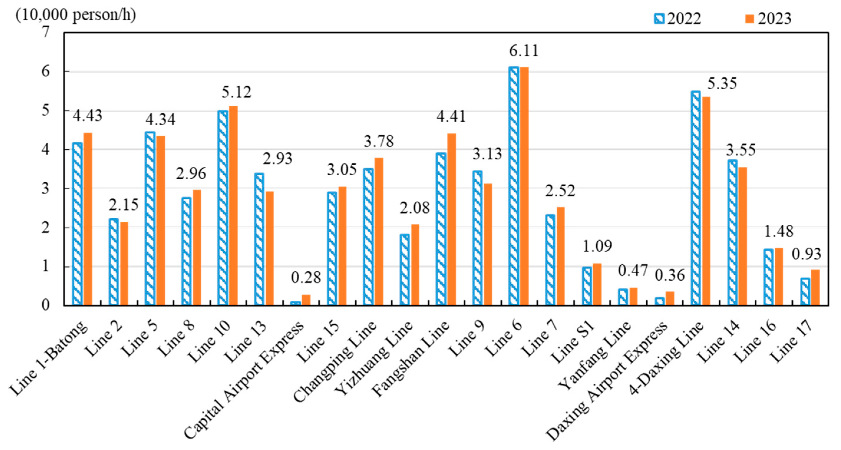
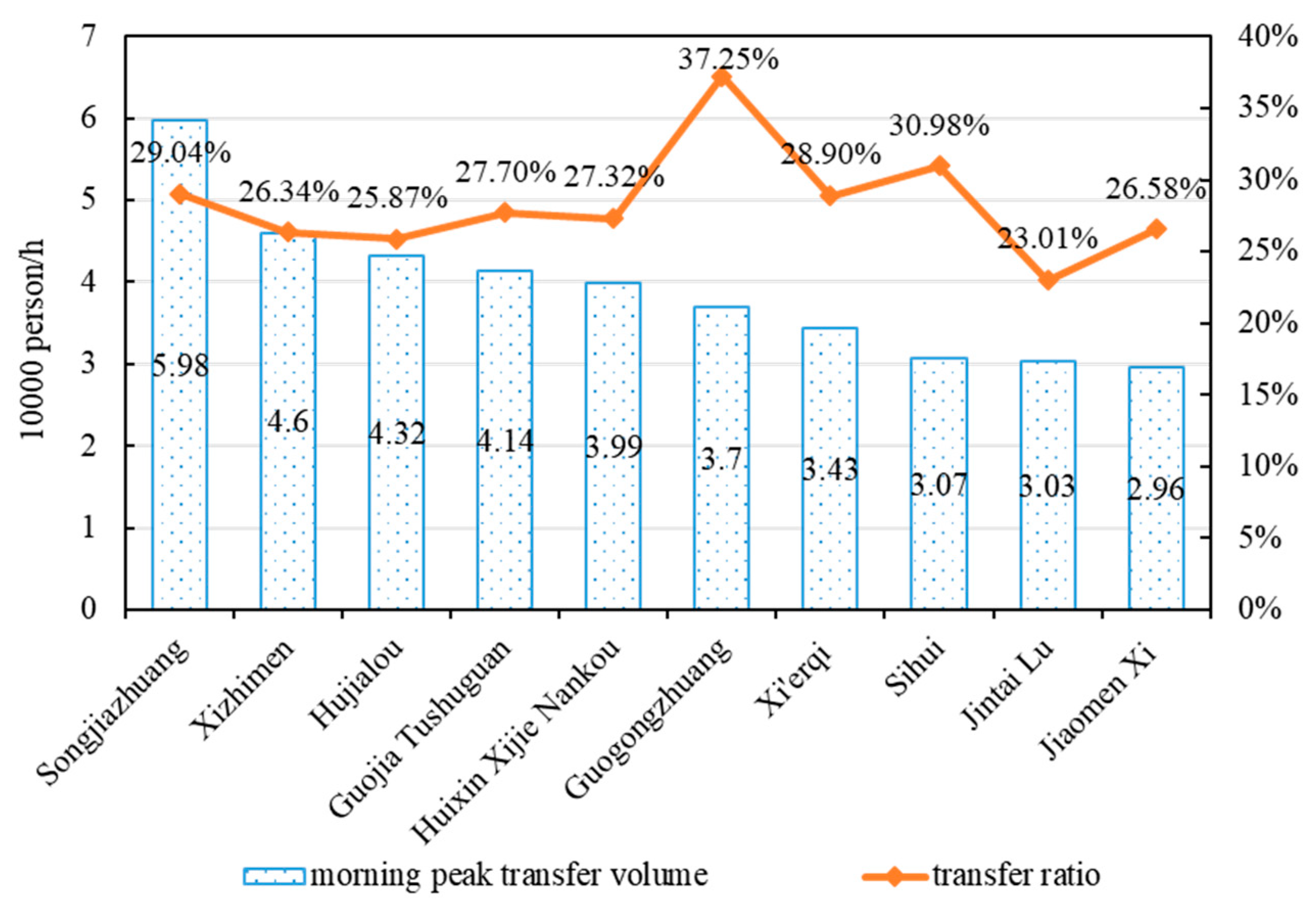
1. Introduction
- The problem of transportation resource sharing under the operation mode of “dedicated line for dedicated trains”
- Limited improvement in the quality and efficiency of rail transit services
- (1)
- The concept of through operation is explored from the perspective of train planning. A new model is developed to plan the train operations for through operation between intercity and high-speed railways. Furthermore, a detailed description of the stop plan under through-operation mode is provided.
- (2)
- An enhanced multi-population genetic algorithm is proposed to solve the train plan problem. It is an innovation in the application of the algorithm.
- (3)
- The method proposed in this paper can meet passenger travel demand under limited-resource conditions, reduce operating costs for the enterprise, and contribute to the long-term and stable development of rail transit.
2. Methodologies
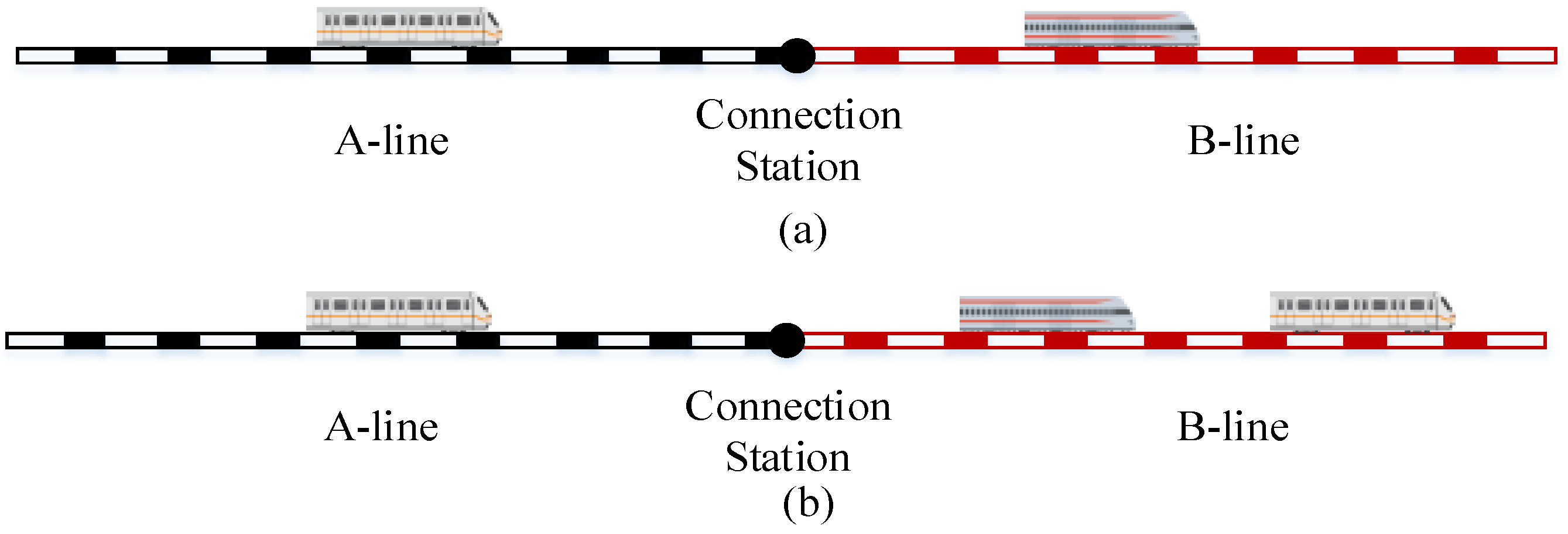
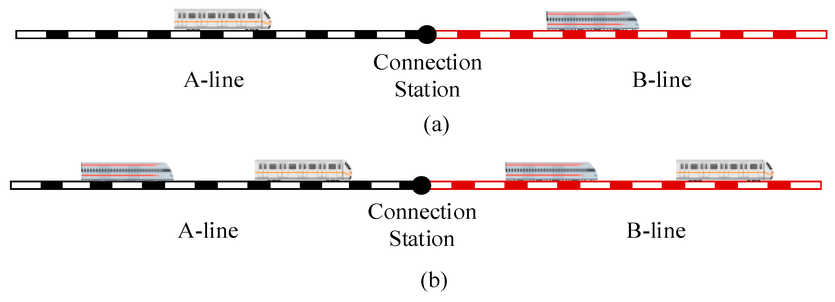
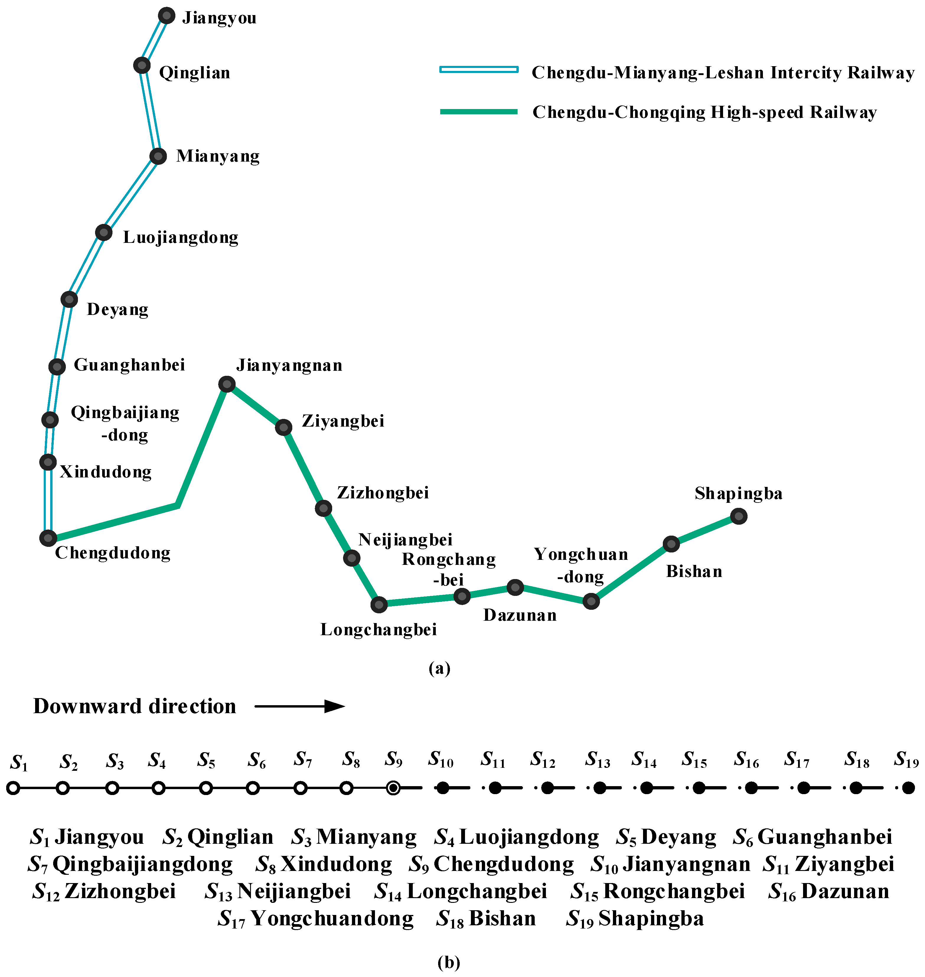
2.1. Problem Description
2.2. Assumptions
- (1)
- Transfer Assumption: Passengers prefer direct travel and will only transfer when there are no direct trains available between two stations. Transfers are allowed only once during the journey.
- (2)
- Unidirectional Assumption: Since high-speed and intercity trains usually operate in pairs for both directions, this study focuses on the train plan in only one direction (downward direction).
- (3)
- Through-Operation Assumption: The two lines are capable of through operation, and some intermediate stations can accommodate turn-back trains. The time for turning back at each station is constant.
- (4)
- Operating Speed Assumption: To maintain line capacity and considering the design speed and the use of EMUs (Electric Multiple Units), high-speed trains should run at the same speed as intercity trains when running on intercity lines. In other words, high-speed trains need to reduce their speed when operating on intercity lines. Due to technical constraints, through-operation intercity trains should maintain their original speed when running on high-speed lines.
- (5)
- Assumption of Train Types: It is assumed that through-operation trains and non- through-operation trains use the same train types. For the sake of differentiation, different symbols and icons are used in the following text, but the actual train types are the same.
2.3. Formulation of the Objective Function
2.3.1. Minimizing Operating Costs for Enterprises
2.3.2. Minimizing Travel Costs for Passengers
2.3.3. Combination of Objective Functions
2.4. Constraints of the Train Plan Model
- 1.
- Passenger demand satisfaction constraint
- 2.
- Available vehicle number constraint
- 3.
- Line capacity constraint
- 4.
- Station service frequency constraint
- 5.
- Position constraint for the through-operation segment
- 6.
- Train stop constraint
- 7.
- Decision variable value constraint
3. Algorithm Design
3.1. Genetic Algorithm Fundamentals
- Algorithm initialization
- 2.
- Fitness evaluation
- 3.
- Selection operation
- 4.
- Crossover operation
- 5.
- Mutation operation
- 6.
- Termination condition
3.2. Design of the Improved Algorithm
- Encoding strategy
- 2.
- Generation of the initial solution
- 3.
- Improvements in crossover and mutation operations
- 4.
- Introduction of the migration operator
3.3. Solving the Process of the Improved Algorithm
- Step 1:
- Import the basic data and set the parameter values of the algorithm. Set the current iteration count to .
- Step 2:
- Enumerate all possible through-operation route schemes . Let the initial through-operation route scheme be . Randomly generated chromosome matrices.
- Step 3:
- Check whether the chromosome matrix satisfies all the constraints.
- Step 4:
- Divide the chromosomes that satisfy all constraints into three populations: A, B, and C. Use Formula (42) to calculate the probability of each chromosome being selected.
- Step 5:
- Randomly pair the selected individuals in pairs. Perform the crossover operation on the paired chromosomes.
- Step 6:
- Perform mutation operations on the selected chromosomes, and the newly generated individuals are screened and corrected.
- Step 7:
- Let , and check whether the iteration count reaches (). If , a migration operator is introduced for interpopulation learning.
- Step 8:
- If , terminate the current iteration and output the optimal solution for the through-operation route, placing it into the candidate set . If , proceed to Step 4.
- Step 9:
- Let . If , proceed to Step 3; otherwise, output the optimal train plan from the candidate set as the global optimal solution.
4. Computation Case and Results Analysis
4.1. Basic Data Settings
4.2. Analysis of Optimal Solution
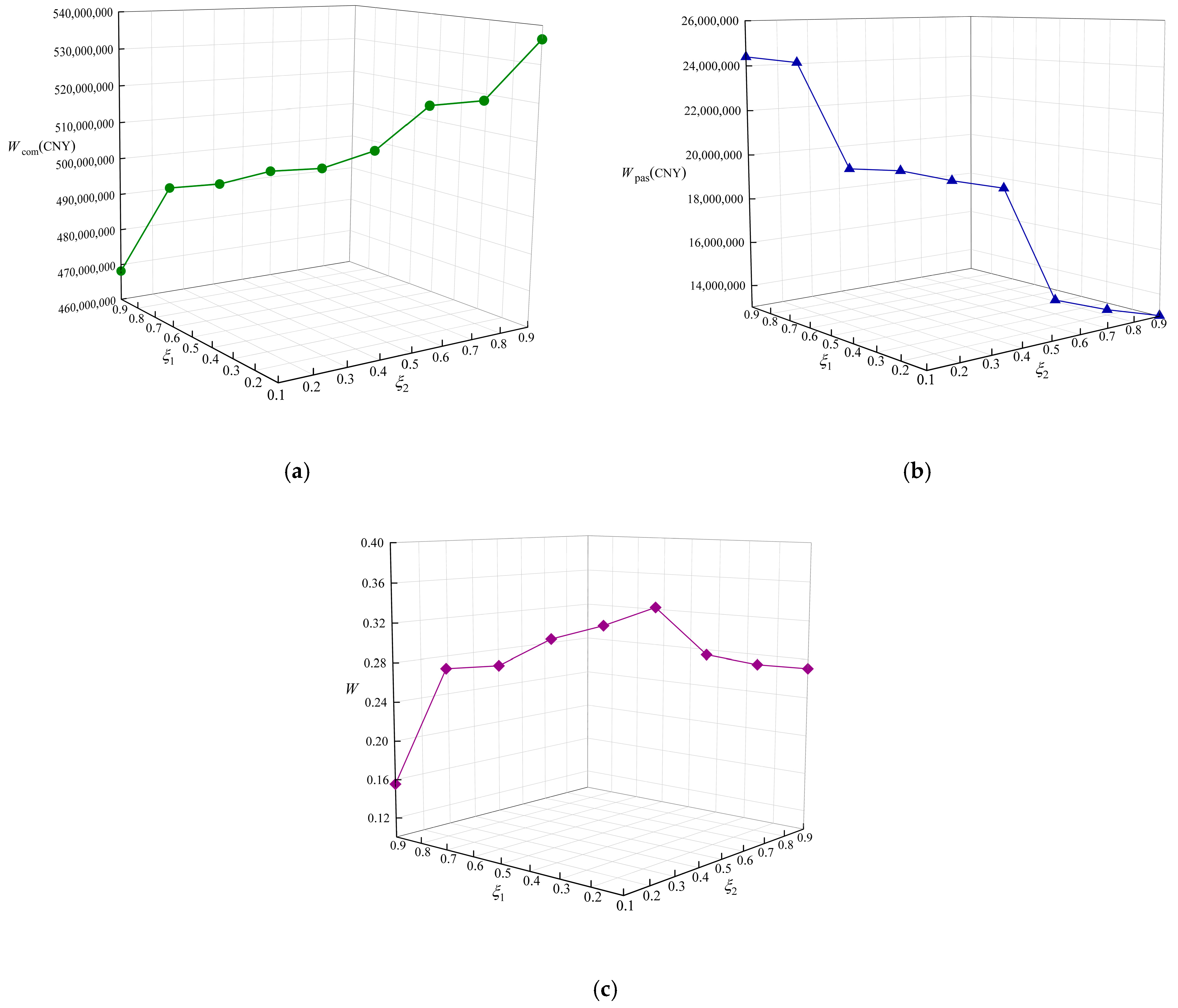
4.2.1. Sensitivity Analysis of Objective Function Weights
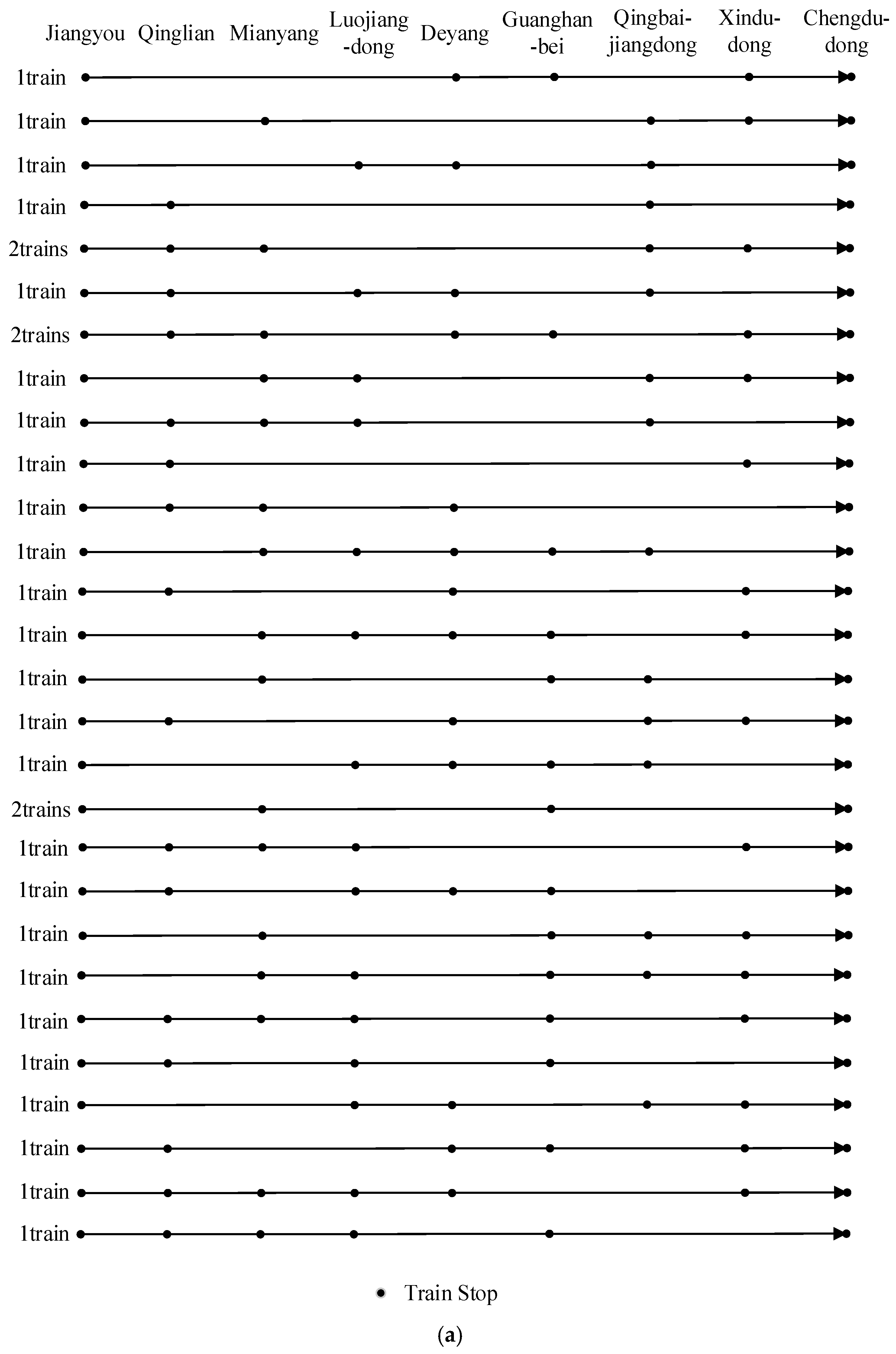
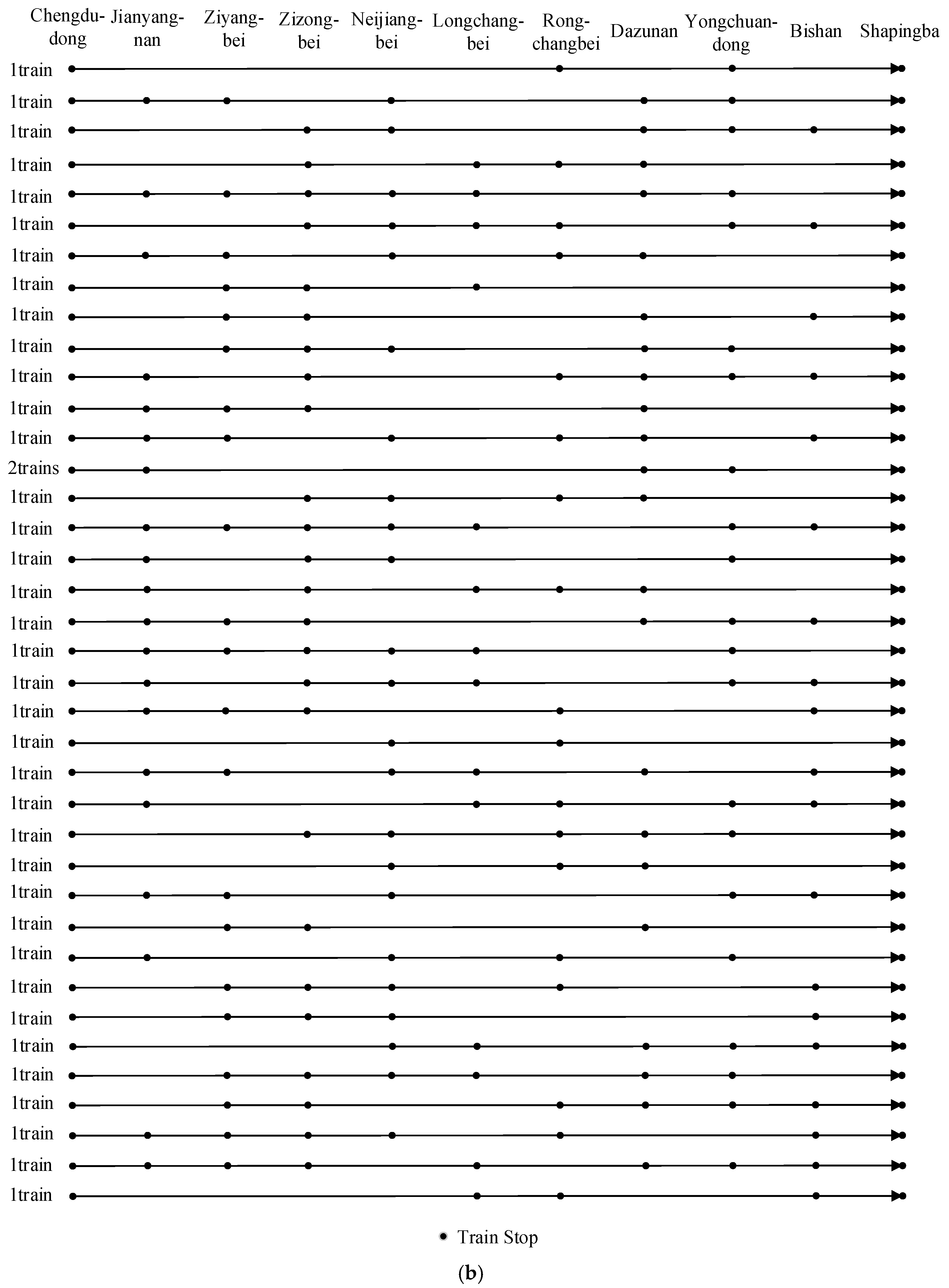
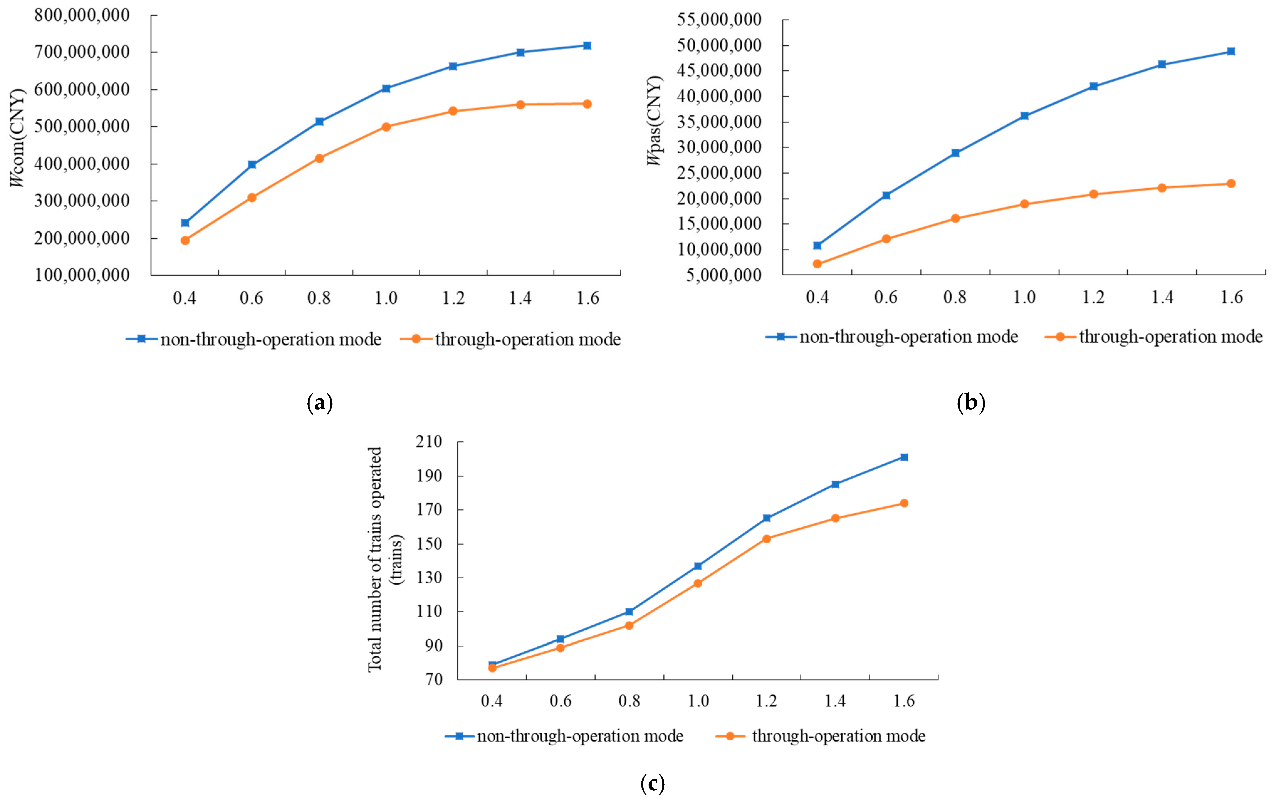
4.2.2. Comparison with Non-Through-Operation Scheme
- Comparison of optimal schemes
- 2.
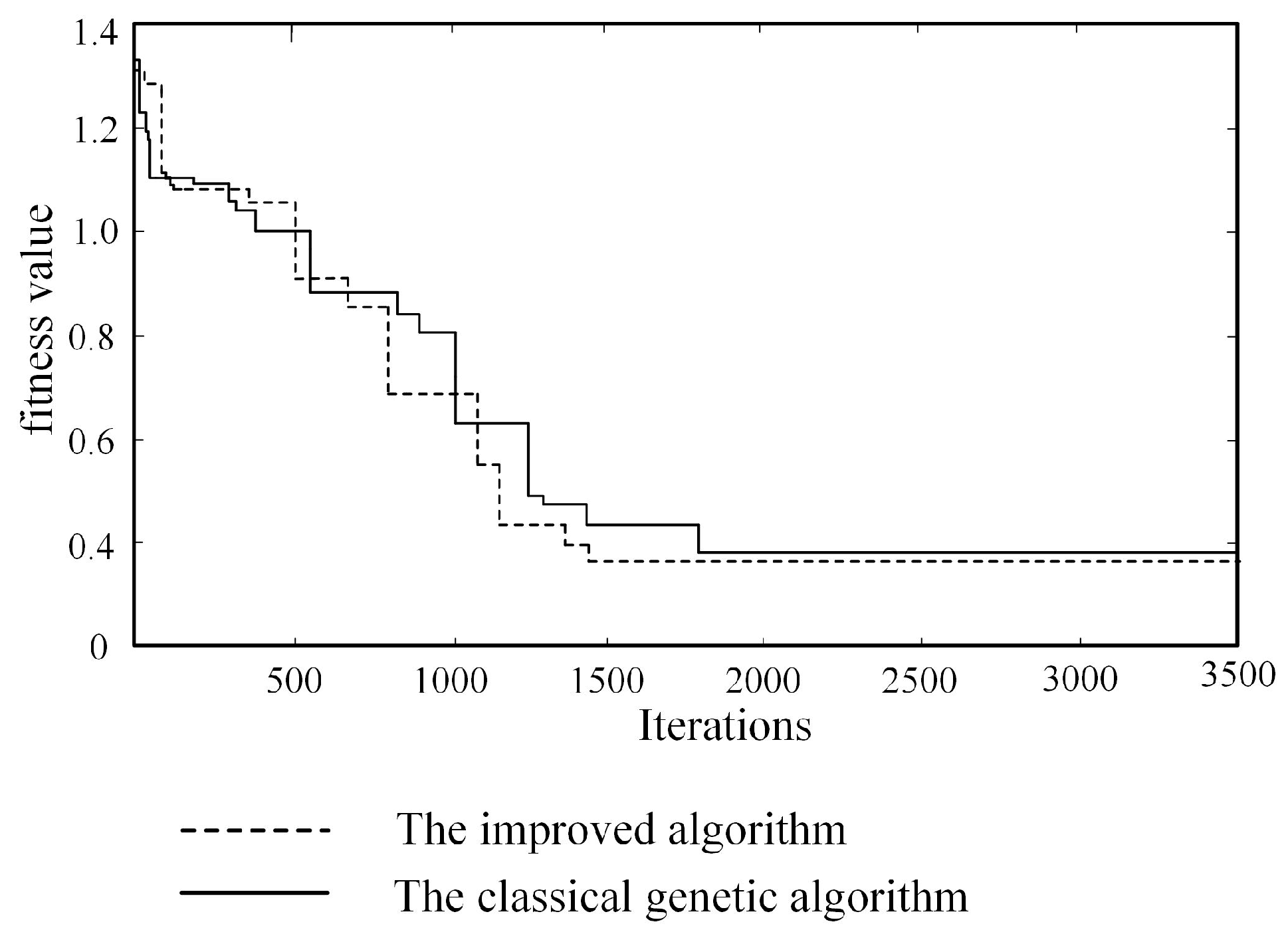
- Comparison with classical genetic algorithm
5. Conclusions
Author Contributions
Funding
Institutional Review Board Statement
Informed Consent Statement
Data Availability Statement
Acknowledgments
Conflicts of Interest
Appendix A

| Symbols | Description | Role |
|---|---|---|
| Set of stations | Set | |
| Set of stations with turnaround capability | Set | |
| Set of intercity trains | Set | |
| Set of through-operation intercity trains | Set | |
| Set of high-speed trains | Set | |
| Set of through-operation high-speed trains | Set | |
| Categories to which train
belongs
| Set | |
| Service frequency of type trains with the same train category, route, and stopping plan. | Decision variable | |
| 0–1 variable. It is 1 if train stops at station , and 0 otherwise. | Decision variable | |
|
0–1 variable. If
is the terminal station of the through-operation intercity train in the downward direction, , else . | Decision variable | |
| 0–1 variable. If is the starting station of the through-operation high-speed train in the downward direction, , else . | Decision variable | |
| Total operating cost of trains during transit | Intermediate variable | |
| Total stopping cost of trains at stations | Intermediate variable | |
| Total travel time cost | Intermediate variable | |
| Total travel ticket cost | Intermediate variable | |
| Travel time for all passengers from Section g to Section l, and | Intermediate variable | |
| Total operating cost of companies | Objective function | |
| Total travel cost of passengers | Objective function | |
| Consolidated overall objective function after transformation | Objective function | |
| Unit vehicle-kilometer cost for type trains | Parameter | |
| Unit stopping cost incurred by -type trains at each station | Parameter | |
| Marshaling number of -type trains | Parameter | |
| Operating mileage of -type trains | Parameter | |
| Fare rate of train | Parameter | |
| Fare rate of train | Parameter | |
| Distance between station and station | Parameter | |
| Distance between station and station | Parameter | |
| Distance between station and station | Parameter | |
| Number of passengers taking train from station to station | Parameter | |
| Number of passengers from station to station who take train and then transfer to train | Parameter | |
| Passengers’ non-working time coefficient | Parameter | |
| Operating speed of trains on intercity rail lines | Parameter | |
| Operating speed of (through-operation) high-speed trains on high-speed rail lines | Parameter | |
| Dwell time of train at intermediate station | Parameter | |
| Dwell time of train at intermediate station | Parameter | |
| Dwell time of train at intermediate station | Parameter | |
| Transfer time per passenger per transfer | Parameter | |
| Number of passengers from station to | Parameter | |
| Capacity of train | Parameter | |
| Average capacity utilization | Parameter | |
| Daily operating duration | Parameter | |
| Turn-back time for trains | Parameter | |
| Maintenance operations time for trains | Parameter | |
| Number of available intercity train vehicles | Parameter | |
| Number of available high-speed train vehicles | Parameter | |
| Maximal capacity of intercity railway line | Parameter | |
| Maximal capacity of high-speed railway line | Parameter | |
| Minimum station service frequency | Parameter | |
| Maximum station service frequency | Parameter |
Appendix B
| Jiangyou | Qinglian | Mianyang | Luojiang- Dong | Deyang | Gunghan-Bei | Qingbai- Jiangdong | Xindu- Dong | Chengdu- Dong | ||
| Jiangyou | 0 | 4236 | 6278 | 4856 | 4327 | 5358 | 5318 | 4535 | 9245 | |
| Qinglian | 5238 | 0 | 4582 | 3414 | 3578 | 3815 | 4078 | 4906 | 6187 | |
| Mianyang | 5499 | 4307 | 0 | 3539 | 4940 | 3798 | 3936 | 4998 | 7770 | |
| Luojiang-dong | 3997 | 4124 | 4447 | 0 | 3971 | 3362 | 3264 | 4168 | 7200 | |
| Deyang | 4215 | 4342 | 4630 | 4134 | 0 | 3570 | 3681 | 4695 | 7266 | |
| Gunghan-bei | 4895 | 3745 | 4237 | 4203 | 4310 | 0 | 3244 | 4818 | 7569 | |
| Qingbai- jiangdong | 4362 | 3765 | 4769 | 3527 | 4951 | 3124 | 0 | 3727 | 6429 | |
| Xindu- dong | 4392 | 4708 | 5508 | 3526 | 4253 | 4653 | 3569 | 0 | 5956 | |
| Chengdu- dong | 7681 | 7219 | 8514 | 6070 | 7682 | 6267 | 8278 | 6942 | 0 | |
| Jianyang- nan | 5911 | 4092 | 3548 | 4054 | 5000 | 4007 | 3190 | 4454 | 8028 | |
| Ziyang- bei | 5059 | 3472 | 3978 | 3274 | 4455 | 2960 | 3324 | 3093 | 6839 | |
| Zizhong- bei | 6635 | 4751 | 6219 | 4735 | 5161 | 5086 | 4950 | 5340 | 6951 | |
| Neijiang- bei | 5252 | 5938 | 5422 | 4778 | 4207 | 5748 | 5057 | 5353 | 6563 | |
| Longchang- bei | 4958 | 3896 | 4234 | 3335 | 4065 | 4076 | 3986 | 4368 | 5719 | |
| Rongchang- bei | 5017 | 4196 | 3940 | 2564 | 3317 | 2512 | 3020 | 3545 | 6495 | |
| Dazu- nan | 4856 | 3950 | 4906 | 3670 | 5030 | 4022 | 3738 | 3873 | 7328 | |
| Yongchuan- dong | 4945 | 4180 | 3632 | 3542 | 3955 | 3688 | 4149 | 5073 | 8334 | |
| Bishan | 4566 | 3072 | 5044 | 3467 | 3682 | 3905 | 4101 | 4972 | 5749 | |
| Shapingba | 4387 | 3226 | 3895 | 2676 | 3210 | 3087 | 2623 | 4153 | 5540 | |
| Jianyang-Nan | Ziyang- Bei | Zizhong- bei | Neijiang- Bei | Longchang- bei | Rongchang- Bei | Dazu- Nan | Yongchuan- Dong | Bishan | Sha-Pingba | |
| Jiangyou | 5055 | 4345 | 7079 | 4964 | 4461 | 4705 | 4797 | 4204 | 5189 | 5067 |
| Qinglian | 3280 | 2875 | 3935 | 4423 | 2980 | 3096 | 4771 | 3532 | 3754 | 3185 |
| Mianyang | 5075 | 3826 | 5611 | 6061 | 5734 | 3828 | 5405 | 4718 | 5423 | 3610 |
| Luojiang-dong | 3354 | 3309 | 4169 | 4206 | 3143 | 2353 | 4008 | 3366 | 3848 | 3184 |
| Deyang | 4149 | 4645 | 6132 | 5386 | 3563 | 3909 | 4636 | 4689 | 4028 | 4038 |
| Gunghan-bei | 3123 | 3691 | 5866 | 4968 | 2923 | 2786 | 3904 | 3471 | 4018 | 2515 |
| Qingbai- jiangdong | 3429 | 3002 | 5750 | 5245 | 3088 | 2828 | 3897 | 3252 | 3320 | 2722 |
| Xindu- dong | 3450 | 3103 | 6194 | 5744 | 3570 | 3979 | 3399 | 4415 | 3503 | 3554 |
| Chengdu- dong | 8021 | 6458 | 7612 | 9111 | 6696 | 5339 | 8393 | 7574 | 6403 | 7437 |
| Jianyang- nan | 0 | 3526 | 4607 | 4141 | 4807 | 4180 | 4164 | 3876 | 5066 | 3539 |
| Ziyang- bei | 3248 | 0 | 4646 | 5186 | 3062 | 2703 | 3357 | 3453 | 4062 | 3321 |
| Zizhong- bei | 4496 | 4944 | 0 | 7533 | 6653 | 4729 | 5554 | 5322 | 6648 | 4122 |
| Neijiang- bei | 5827 | 5344 | 6297 | 0 | 4575 | 4585 | 4541 | 5818 | 4710 | 5021 |
| Longchang- bei | 3467 | 4202 | 6592 | 4520 | 0 | 3105 | 3950 | 3579 | 4290 | 4094 |
| Rongchang- bei | 3948 | 2247 | 4823 | 3635 | 3513 | 0 | 3635 | 2805 | 2851 | 2940 |
| Dazu- nan | 3856 | 3005 | 6420 | 4688 | 3443 | 3436 | 0 | 3518 | 4847 | 3656 |
| Yongchuan- dong | 3716 | 3680 | 5671 | 5089 | 4285 | 3633 | 3548 | 0 | 4951 | 3910 |
| Bishan | 3434 | 4178 | 4962 | 4720 | 4726 | 3276 | 4254 | 5026 | 0 | 3234 |
| Shapingba | 3885 | 2362 | 5000 | 4766 | 3405 | 3100 | 3464 | 3993 | 2861 | 0 |
References
- Zhou, Y.; Yang, H.; Wang, Y.; Yan, X.D. Integrated Line Configuration and Frequency Determination with Passenger Path Assignment in Urban Rail Transit Networks. Transp. Res. B Methodol. 2021, 145, 134–151. [Google Scholar] [CrossRef]
- Feng, T.; Tao, S.Y.; Li, Z.Y. Optimal Operation Scheme with Short-Turn, Express, and Local Services in an Urban Rail Transit Line. J. Adv. Transport. 2020, 2020, 830593. [Google Scholar] [CrossRef]
- Cao, Z.C.; Ceder, A.; Li, D.W.; Zhang, S.L. Robust and Optimized Urban Rail Timetabling Using a Marshaling Plan and Skip-Stop Operation. Transp. A Transp. Sci. 2020, 23, 1217–1249. [Google Scholar] [CrossRef]
- Oh, S.; Choi, J.W. An Optimization Method to Design a Skip-stop Pattern for Renovating Operation Schemes in Urban Railways. Transp. Lett. 2022, 14, 909–919. [Google Scholar] [CrossRef]
- Cerdeira, J.O.; Iglésias, C.; Silva, P.C. The Train Frequency Compatibility Problem. Discrete. Appl. Math. 2019, 269, 18–26. [Google Scholar] [CrossRef]
- Canca, D.; Barrena, E.; De-Los-Santos, A.; Andrade-Pineda, J.L. Setting Lines Frequency and Capacity in Dense Railway Rapid Transit Networks with Simultaneous Passenger Assignment. Transp. Res. B Methodol. 2016, 93, 251–267. [Google Scholar] [CrossRef]
- Sun, Y.H.; Cao, C.X.; Wu, C. Multi-Objective Optimization of Train Routing Problem Combined with Train Scheduling on a High-Speed Railway Network. Transp. Res. C Emerg. Technol. 2014, 44, 1–20. [Google Scholar] [CrossRef]
- Dolgopolov, P.; Konstantinov, D.; Pybalchenko, L.; Muhitovs, R. Optimization of Train Routes Based on Neuro-Fuzzy Modeling and Genetic Algorithms. ICTE Transp. Logist. 2019, 149, 11–18. [Google Scholar] [CrossRef]
- Yan, S.H.; Zhang, T.W.; Dong, L.J. Optimization Model of Operation Route Selection of High Speed Railway Cross-Line Trains. Rail. Transp. Econ. 2021, 43, 109–116. [Google Scholar]
- Duan, B.T. Analysis of Urban Rail Transit Train Passing Capacity Based on Flexible Formation Mode. Urban. Mass. Transp. 2023, 26, 118–124. [Google Scholar]
- Tai, G.X.; Huang, Y.N.; Li, C.C.; Wang, X. An Optimization Method of Train Scheduling for Urban Rapid Rail Transit Based on Flexible Train Composition Mode. J. Transp. Syst. Eng. Inf. Technol. 2023, 23, 195–203. [Google Scholar]
- You, T.; Ma, F.Y.; Miao, F.; Xu, G.D.; Yang, Z.P. Optimal Operation Plan Design for Virtually Coupled Trains in Urban Rail Transit. Urban. Rapid. Rail. Transp. 2023, 36, 36–42. [Google Scholar]
- Schöbel, A. An Eigenmodel for Iterative Line Planning, Timetabling and Vehicle Scheduling in Public Transportation. Transp. Res. C Emerg. Technol. 2017, 74, 348–365. [Google Scholar] [CrossRef]
- Zhang, Y.X.; Peng, Q.Y.; Lu, G.Y.; Zhong, Q.W.; Zan, X.; Zhou, X.S. Integrated Line Planning and Train Timetabling Through Price-Based Cross-Resolution Feedback Mechanism. Transp. Res. B Methodol. 2022, 155, 240–277. [Google Scholar] [CrossRef]
- Tang, J.J.; Yang, L.P.; Zhou, L.S. Optimal Planning Method for Operation Plan of Through Train Based on Dynamic Traffic Assignment of Service Network. China Rail. Sci. 2016, 37, 115–120. [Google Scholar]
- Shi, F.; Li, Y.L.; Hu, X.L.; Xu, G.M.; Shan, X.H. Service Level Oriented Optimization of Train Operation Plan for High Speed Railway. China Rail. Sci. 2018, 39, 127–136. [Google Scholar]
- Meng, X.L.; Qin, Y.; Jia, L.M. Comprehensive Evaluation of Passenger Train Service Plan Based on Complex Network Theory. Measurement 2014, 58, 221–229. [Google Scholar] [CrossRef]
- Mao, B.H.; Zhang, Z.; Chen, Z.J.; Jia, W.Z.; He, T.J. A Review on Operational Technologies of Urban Rail Transit Networks. J. Transp. Syst. Eng. Inf. Technol. 2017, 17, 155–163. [Google Scholar]
- Huang, Q.S.; Chen, Y.; Zhang, A.Y.; Zhou, Q.; Bai, Y.; Mao, B.H. Optimization of urban rail network operation scheme considering interconnection. J. Railw. Sci. Eng. 2023, 20, 1587–1597. [Google Scholar]
- Sun, M.X.; Ni, S.Q.; Lv, H.X. Rail Transit Optimization for Train Operation Plan under Network Operation. J. Transp. Eng. Inf. 2020, 18, 26–33+60. [Google Scholar]
- Lópezramos, F.; Codina, E.; Marinín, Á.; Guarnaschelli, A. Integrated Approach to Network Design and Frequency Setting Problem in Railway Rapid Transit Systems. Comput. Oper. Res. 2017, 80, 128–146. [Google Scholar] [CrossRef]
- Yang, A.A.; Wang, B.; Huang, J.L.; Li, C. Service Replanning in Urban Rail Transit Networks: Cross-Line Express Trains for Reducing the Number of Passenger Transfers and Travel Time. Transp. Res. C Emerg. Technol. 2020, 115, 102629. [Google Scholar] [CrossRef]
- Huang, K.; Liao, F.X.; Gao, Z.Y. An Integrated Model of Energy-Efficient Timetabling of the Urban Rail Transit System with Multiple Interconnected Lines. Transp. Res. C Emerg. Technol. 2021, 129, 103171. [Google Scholar] [CrossRef]
- Zeng, Q.W.; Peng, Q.Y. Cross-Line Train Plan in Urban Rail Transit Considering the Multi-Group Train. J. Railw. Sci. Eng. 2023, 20, 878–889. [Google Scholar]
- Feng, Y.H.; Lv, H.X.; Huang, J.X.; Lv, M.M. Train Planning for Through Operation between Subway and Suburban Railway. J. Transp. Eng. Inf. 2021, 19, 96–100. [Google Scholar]
- Li, M.G.; Liu, J.F.; Liu, X.H.; Wang, J.; Li, J.H. Train Planning for Through Operation between Subway and Suburban Railway. J. Transp. Syst. Eng. Inf. Technol. 2017, 17, 178–184. [Google Scholar]
- Lin, L.; Meng, X.L.; Cheng, X.Q.; Ma, Y.Y.; Xu, S.C.; Han, Z. Line planning under the operation mode of line sharing between metro and suburban railway. J. Adv. Transport. 2023, 2023, 8847456. [Google Scholar] [CrossRef]
- Chen, Y.J.; Liu, X.M.; Rao, M.; Qin, Y.; Wang, Z.P.; Ji, Y.J. Explicit speed-integrated LSTM network for non-stationary gearbox vibration representation and fault detection under varying speed conditions. Reliab. Eng. Syst. Safe. 2025, 254, 110596. [Google Scholar] [CrossRef]
- Ji, Y.J.; Huang, Y.P.; Zeng, J.W.; Ren, L.H.; Chen, Y.J. A physical-data-driven combined strategy for load identification of tire type rail transit vehicle. Reliab. Eng. Syst. Safe. 2025, 253, 110493. [Google Scholar] [CrossRef]
- Yang, Q. Study on Optimization of High-Speed Train Line Planning Considering the Mixed Operation Mode of this and Cross Line Trains. Ph.D. Thesis, Beijing Jiaotong University, Beijing, China, 2022. [Google Scholar]
- Wu, X.T.; Yang, M.K.; Wang, H.W.; Lv, J.H.; Dong, H.R. Load-balancing oriented line plan optimization for a high-speed railway network. Acta Autom. Sin. 2022, 48, 492–503. [Google Scholar]
| City | Passenger Volume [×10,000] | Entry Volume [×10,000] | Maximum Daily Passenger Volume of the Line [×10,000] | Maximum Daily Passenger Volume of the Station [×10,000] |
|---|---|---|---|---|
| Beijing | 345,294.26 | 190,296.03 | 183.54 | 45.76 |
| Shanghai | 366,906.65 | 202,888.93 | 144.60 | 68.80 |
| Tianjin | 57,132.93 | 35,661.96 | 55.10 | 33.03 |
| Chongqing | 132,582.81 | 83,377.33 | 93.67 | 37.95 |
| Guangzhou | 313,413.28 | 171,501.20 | 236.65 | 77.74 |
| Shenzhen | 271,112.14 | 158,890.28 | 139.37 | 60.33 |
| Wuhan | 135,163.39 | 85,652.12 | 138.29 | 45.23 |
| Nanjing | 100,998.93 | 61,028.79 | 120.66 | 74.32 |
| Chengdu | 212,191.00 | 120,161.00 | 106.00 | 52.58 |
| Hangzhou | 138,357.17 | 82,857.29 | 124.56 | 36.49 |
| Parameter | Value | Measurement Unit |
|---|---|---|
| , , , | 75, 75, 80, 80 | CNY/vehicle·km |
| , , , | 450, 450, 500, 500 | CNY/train·station |
| , , , | 8, 8, 8, 8 | Vehicle |
| , , , | 0.4, 0.4, 0.5, 0.5 | CNY/person·km |
| 25 | CNY/h | |
| , | 250, 300 | Km/h |
| 0.25 | h | |
| , , | 0.05, 0.05, 0.05 | h |
| , , , | 610, 610, 494, 494 | Person |
| 0.75 | - | |
| , , , | 0.17, 0.25, 0.33, 0.42 | h |
| , , , | 0.5, 0.5, 0.75, 0.75 | h |
| 16 | h | |
| , | 480, 620 | Vehicle |
| , | 144, 144 | Trains/day |
| Parameter | Definition | Value |
|---|---|---|
| Amplification factor | 1000 | |
| Penalty factor | 1000 | |
| Population size | 50 | |
| Baseline crossover probability | 0.8 | |
| Baseline mutation probability | 0.1 | |
| Baseline number of mutation points | 6 | |
| Migration interval | 10 | |
| Migration probability | 0.3 | |
| Maximum number of iterations | 3500 |
| (0.1, 0.9) | 38 | 19 | 25 | 54 | 536,482,170 | 13,028,074.87 | 0.270526 | ||
| (0.2, 0.8) | 29 | 27 | 40 | 39 | 520,094,820 | 13,242,495.94 | 0.275129 | ||
| (0.3, 0.7) | 38 | 24 | 40 | 42 | 518,215,950 | 13,629,969.87 | 0.285876 | ||
| (0.4, 0.6) | 32 | 36 | 30 | 43 | 505,613,220 | 18,636,557.94 | 0.334503 | ||
| (0.5, 0.5) | 31 | 19 | 39 | 38 | 500,149,230 | 18,943,237.99 | 0.316196 | ||
| (0.6, 0.4) | 20 | 33 | 33 | 42 | 498,663,480 | 19,361,447.88 | 0.302926 | ||
| (0.7, 0.3) | 30 | 30 | 26 | 45 | 494,401,110 | 19,422,301.39 | 0.276259 | ||
| (0.8, 0.2) | 24 | 40 | 28 | 39 | 492,552,690 | 24,154,043.66 | 0.273703 | ||
| (0.9, 0.1) | 30 | 33 | 28 | 37 | 468,172,110 | 24,400,748.18 | 0.155434 |
| 3 | 12 | 31 | 19 | 39 | 38 | 500,149,230 | 189,43,237.99 | 0.316196 |
| - | - | 64 | - | 73 | - | 6,035,83,050 | 36,156,921.48 | 0.821191 |
| Comparison Items | The Improved Algorithm | The Classical Genetic Algorithm |
|---|---|---|
| Iteration count | 1453 | 1790 |
| 0.316196 | 0.342535 | |
| 500,149,230 | 514,139,430 | |
| 18,943,237.99 | 18,679,335.90 | |
| Operation sections of through- operation intercity trains | ||
| Operation sections of through- operation high-speed trains | ||
| 31 | 31 | |
| 19 | 40 | |
| 39 | 38 | |
| 38 | 35 |
Disclaimer/Publisher’s Note: The statements, opinions and data contained in all publications are solely those of the individual author(s) and contributor(s) and not of MDPI and/or the editor(s). MDPI and/or the editor(s) disclaim responsibility for any injury to people or property resulting from any ideas, methods, instructions or products referred to in the content. |
© 2025 by the authors. Licensee MDPI, Basel, Switzerland. This article is an open access article distributed under the terms and conditions of the Creative Commons Attribution (CC BY) license (https://creativecommons.org/licenses/by/4.0/).
Share and Cite
Lin, L.; Meng, X.; Song, K.; Feng, L.; Han, Z.; Xia, X. Train Planning for Through Operation Between Intercity and High-Speed Railways: Enhancing Sustainability Through Integrated Transport Solutions. Sustainability 2025, 17, 1089. https://doi.org/10.3390/su17031089
Lin L, Meng X, Song K, Feng L, Han Z, Xia X. Train Planning for Through Operation Between Intercity and High-Speed Railways: Enhancing Sustainability Through Integrated Transport Solutions. Sustainability. 2025; 17(3):1089. https://doi.org/10.3390/su17031089
Chicago/Turabian StyleLin, Li, Xuelei Meng, Kewei Song, Liping Feng, Zheng Han, and Ximan Xia. 2025. "Train Planning for Through Operation Between Intercity and High-Speed Railways: Enhancing Sustainability Through Integrated Transport Solutions" Sustainability 17, no. 3: 1089. https://doi.org/10.3390/su17031089
APA StyleLin, L., Meng, X., Song, K., Feng, L., Han, Z., & Xia, X. (2025). Train Planning for Through Operation Between Intercity and High-Speed Railways: Enhancing Sustainability Through Integrated Transport Solutions. Sustainability, 17(3), 1089. https://doi.org/10.3390/su17031089