Article

Identification of Local and Transboundary Sources and Mechanisms of PM2.5 and O3 Pollution on the Tibetan Plateau: Implications for Sustainable Air Quality Governance

1
School of Remote Sensing and Information Engineering, North China Institute of Aerospace Engineering, Langfang 065000, China
2
Institute of Geographic Sciences and Natural Resources Research, Beijing 100101, China
3
Qinghai Provincial Center for Environmental Planning and Environmental Protection Technology, Xining 810000, China
4
College of Resources and Environment, University of Chinese Academy of Sciences, Beijing 100049, China
5
Beijing Yanshan Earth Critical Zone National Research Station, University of Chinese Academy of Sciences, Beijing 101400, China
*
Author to whom correspondence should be addressed.
Sustainability 2025, 17(23), 10853; https://doi.org/10.3390/su172310853
Submission received: 29 September 2025 / Revised: 13 November 2025 / Accepted: 1 December 2025 / Published: 3 December 2025
(This article belongs to the Special Issue Air Pollution: Causes, Monitoring and Sustainable Control)

Abstract

Air pollution, particularly fine particulate matter (PM2.5) and ozone (O3) pollution, poses serious challenges to environmental quality and sustainable development. The Tibetan Plateau, often described as the “Third Pole,” functions as a key ecological shield for China and exerts wide-reaching influence on global climate systems, hydrological cycles, and cross-regional pollution transport. To better clarify the driving mechanisms of air pollution in this sensitive region, we propose an integrated MRG–HSW framework, which, for the first time, systematically couples statistical modeling and trajectory analysis by combining multivariate regression, residual-based screening, and HYSPLIT–WCWT trajectory analyses. Taking Qinghai Province as a case study, ERA5 and GDAS1 reanalysis products were coupled with in situ monitoring to identify the relative contributions of local emissions and long-range atmospheric transport. The results show that, in low-elevation zones, PM2.5 levels are largely governed by local anthropogenic activities (R2 = 0.631–0.803), whereas O3 concentrations respond more strongly to meteorological variability (R2 = 0.529–0.779). At higher elevations, however, local explanatory factors weaken, and long-range transport from the Hexi Corridor, Qaidam Basin, and even South Asia becomes the dominant influence for both pollutants. Additional sensitivity tests confirm that the framework performs robustly under diverse meteorological and seasonal conditions. Collectively, this work not only establishes a transferable methodology for source attribution in plateau environments but also underscores the pivotal role of the Tibetan Plateau in sustaining regional air quality and global environmental stability.

1. Introduction

In recent years, PM2.5 and O3 have been identified as two significant global air pollutants, presenting severe risks to human health and exerting substantial effects on ecological systems [1,2]. In response to acute air pollution issues, China initiated the Air Pollution Prevention and Control Action Plan in 2013, which aimed to enhance air quality via rigorous emission reduction strategies. Subsequent monitoring data revealed that, after the implementation of this plan, anthropogenic PM2.5 emissions diminished by approximately 33%, which corresponded with a marked amelioration in levels of particulate pollution [3,4]. However, surface O3 concentrations continued to rise, increasing by about 7.5% nationwide from 2015 to 2024 according to the China Ecological and Environmental Status Bulletin [5,6,7]. These findings highlight the ongoing challenge of jointly controlling PM2.5 and O3 pollution despite notable emission reductions [8].
In recent years, studies on the local attribution of PM2.5 and O3 pollution have shifted from empirical statistics toward multi-source integration and process-based interpretation. Early works mainly employed multiple linear regression (MLR) models to quantify the linear responses of pollutants to meteorological and emission factors. These models are simple and highly interpretable, enabling clear identification of key drivers and their contribution directions. For instance, national-scale trend analyses have shown that the decline in PM2.5 concentrations was primarily driven by emission reductions, while O3 variations were jointly influenced by meteorological conditions and photochemical processes [9]. At the urban scale, MLR has been used to reveal the differentiated impacts of temperature, humidity, wind speed, and boundary layer height on PM2.5 and O3, providing quantitative evidence for local air pollution control [10]. As understanding of nonlinear responses has deepened, the generalized additive model (GAM) has been introduced to overcome the linearity assumption of MLR. By using nonparametric smoothing functions, GAM captures nonlinear and threshold effects of meteorological variables, significantly improving explanatory power and fitting accuracy. Studies have identified a “threshold-enhancing” effect of temperature, solar radiation, and boundary layer height on O3, while wind speed and precipitation exhibit “cleansing-dilution” patterns [11]. Compared with gradient boosting models (GBM) and other machine learning approaches, GAM shows greater advantages in causal interpretation and physical consistency [12]. In recent years, machine learning methods have been widely applied for multi-source data fusion and factor importance analysis. Models such as CatBoost, XGBoost, and random forest (RF) can identify major driving factors within complex multidimensional datasets and quantify their contributions, revealing nonlinear relationships between pollutants, meteorological, and socioeconomic factors [13,14]. Distributed lag nonlinear models (DLNM) further describe the lagged effects of meteorological variables [15]. However, despite their high accuracy, machine learning approaches often suffer from limited physical interpretability and strong dependence on sample size, particularly in data-scarce or topographically complex regions. To balance physical constraints and statistical flexibility, researchers have proposed hybrid statistical–physical frameworks that combine outputs from chemical transport models (CTMs) such as GEOS-Chem and WRF-Chem for bias correction and weighted integration, effectively reducing prediction errors [16]. Overall, local attribution studies are evolving from traditional linear statistics toward multi-source information fusion and mechanism-based modeling. Given the need for interpretability and robustness under data-scarce conditions, this study employs MLR and GAM to quantify both linear and nonlinear relationships between meteorological drivers and pollutant concentrations, ensuring physically consistent and mechanism-oriented analysis suitable for the Tibetan Plateau.
Meanwhile, research on external transport of air pollution has developed into a multi-level framework centered on trajectory analysis, concentration-weighted trajectory models (PSCF/CWT/WCWT), and CTMs. Receptor-based approaches using backward trajectories remain classical tools for identifying cross-regional transport pathways, typically employing the HYSPLIT model to compute 72 h trajectories and conduct clustering analyses that reveal dominant airflow channels [17]. Such clustering has been applied not only in urban environments but also in mountainous and plateau regions to distinguish between long-range and short-range seasonal transport [18,19]. The choice of clustering algorithm can influence pathway classification [20], while the integration of mobile and multi-site observations enhances spatial resolution [21]. For source region identification, weighted trajectory models link high concentration events with trajectory endpoints to highlight potential source areas [19]. The concentration-weighted trajectory (CWT) method has been widely applied to integrate satellite and ground-based observations for identifying major source regions [22], though its stability is sensitive to sampling resolution [23]. The weighted concentration-weighted trajectory (WCWT) further introduces concentration-weighted averaging, enabling finer quantifications of grid-level contributions and complementing clustering results; self-organizing maps (SOM) emphasize “path structures,” whereas WCWT focuses on “potential source regions” [21]. Chemical transport models such as WRF-Chem, CMAQ/CAMx, and GEOS-Chem can mechanistically evaluate emissions, transport, and chemical processes [24,25], though their application is often constrained by the need for detailed emission inventories and high computational demand, especially in data-limited regions like the Tibetan Plateau. Recent studies have combined numerical simulations with trajectory-based statistics to improve transport pathway identification [26,27], and hybrid approaches integrating “CTM + trajectory/receptor + machine learning” are emerging as efficient and interpretable tools for source attribution. Considering the sparse observation network and complex airflow over the Plateau, this study integrates HYSPLIT and WCWT analyses to trace transport pathways and identify dominant external source regions, providing a physically grounded yet computationally efficient approach to characterize transboundary influences.
Taken together, these developments demonstrate a clear methodological shift from single-technique analyses toward integrated frameworks that couple local and regional processes. Yet, most existing studies remain focused on lowland urban areas, with limited exploration of how local meteorology, emissions, and long-range transport interact under the complex topography and low-emission conditions of the Tibetan Plateau. To fill this gap, an integrated approach that links statistical interpretation with physical process representation is required to better distinguish local contributions from external transport influences.
To address these gaps, this study takes Qinghai Province as a representative region of the Tibetan Plateau and develops an integrated statistical–trajectory framework (MRG–HSW) that links local attribution with regional transport analysis. The goal is to better understand the mechanisms that drive PM2.5 and O3 pollution over the Tibetan Plateau. Specifically, the study aims to:
(1)
Develop an integrated MRG–HSW framework that couples statistical modeling with trajectory-based diagnostics;
(2)
Quantify the effects of local meteorological and emission-related factors on local pollutant concentrations;
(3)
Identify dominant source regions and transport pathways during high-pollution episodes;
(4)
Evaluate elevation-dependent mechanisms to support evidence-based and cooperative air-quality governance in complex plateau terrain.
Overall, this study contributes a systematic and scalable analytical framework that advances the understanding of pollution formation on the Tibetan Plateau and offers new scientific evidence for regional emission mitigation and transboundary air pollution management.

2. Materials and Methods

This study explores the formation mechanisms of PM2.5 and O3 pollution in Qinghai Province, located in the northeastern part of the Tibetan Plateau, which exhibits typical plateau characteristics and provides comprehensive air quality monitoring data. Therefore, it can serve as a representative region for studying the atmospheric environmental characteristics of the broader Tibetan Plateau. Qinghai Province, situated at the transition zone of the Plateau, shares similar geographical, climatic, and ecological conditions with the Plateau’s main area, and has high data continuity. Thus, selecting Qinghai as the study area effectively represents the pollution characteristics and formation mechanisms of the entire Tibetan Plateau. Analyses were conducted across eight prefecture-level regions, as illustrated in Figure 1.

2.1. Meteorological and Pollutant Data

The investigation covers the period from 2020 to 2024, encompassing air pollutant concentrations and meteorological data, including driver fields.
Hourly air pollutant data were collected from eight cities via CNEMC. Missing data points were imputed following a hierarchical strategy: gaps of 1–3 h were linearly interpolated, 4–6 h gaps were filled using a centered 5 h moving average, and 7–24 h gaps were replaced by the mean of the same hour from the preceding and following three years. The dataset was rigorously cleansed before any analytical procedures were performed. Subsequently, the daily mean concentrations of PM2.5, PM10, SO2, NO2, and CO were calculated. For O3, the maximum daily 8 h average (MDA8) was derived from the processed hourly data. Considering the underestimation and uncertainties in emission inventories over the Tibetan Plateau, ground-based pollutant concentrations were used as proxies for local anthropogenic emissions. This validated approach helps improve the reliability of source attribution [28,29,30,31,32]. Meteorological data were obtained from the ERA5 reanalysis dataset (ECMWF). Hourly ERA5 data were matched to each monitoring site using the nearest-neighbor method. Daily variables-relative humidity (rh), boundary layer height (blh), surface solar radiation (ssrd), 2 m air temperature (t2m), total precipitation (tp), and wind speed (wind)-were calculated by averaging hourly values (for t2m, rh, blh, wind) and summing accumulative ones (for tp, ssrd). This ensured temporal and spatial consistency with the pollutant data. These ERA5 variables were used only as predictors in the MLR model. Although potential site-level biases may exist, previous studies have shown that ERA5 provides reliable temporal consistency over the Tibetan Plateau [33,34,35]. Meteorological fields for trajectory simulations were derived from the GDAS1 reanalysis dataset released by NCEP. For each monitoring site, 72 h backward trajectories were simulated using the HYSPLIT model at multiple altitudes (500 m, 1000 m, 1500 m) and four commencement times per day (00, 06, 12, and 18 UTC). To maintain temporal consistency, trajectories were aligned by start time and matched with the daily pollutant values of the same day. The trajectories thus generated formed the foundation for subsequent analyses. Table 1 presents a comprehensive summary of all datasets, variables, and their sources used in this study.

2.2. Integrated Methodology: The MRG-HSW Attribution Framework

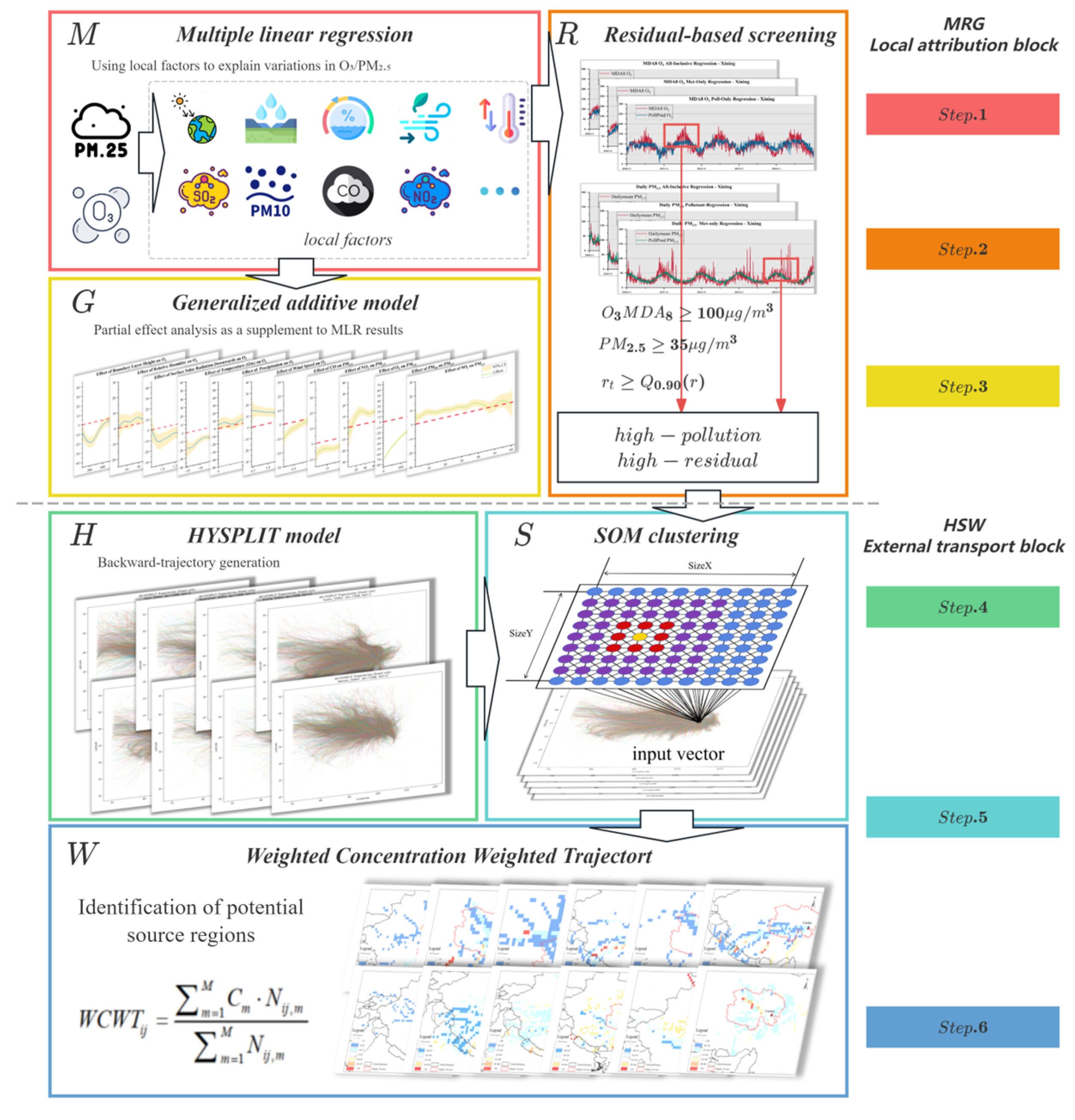
To systematically elucidate the local drivers and external influences on PM2.5 and O3 concentrations over the Tibetan Plateau, this study introduces the MRG–HSW integrated attribution framework, which comprises two primary components—the local attribution module (MRG) and the external transport diagnostic module (HSW). A schematic overview is provided in Figure 2, while detailed descriptions are presented in Section 2.2.1 and Section 2.2.2.

2.2.1. Local Attribution Block: MRG

M (Multiple linear regression, MLR): The MLR model is favored for its simplicity and interpretability and is extensively utilized in environmental research, offering clearer physical insights compared with the black-box nature of most machine learning and deep learning models [36,37]. Variations in PM2.5 and O3 concentrations are primarily influenced by local meteorological conditions and co-emitted pollutants [38,39,40,41,42], with potential modifications stemming from external transport. This research constructed three distinct types of models: meteorological-factor models, pollutant factor models, and combined models. These models are employed to compare the goodness of fit and statistical significance among various combinations of factors, thereby determining the relative contributions of each. The performance of these models was assessed using adjusted R2 (to gauge explanatory power), t-values (to rank the influence strength of variables), and Variance Inflation Factors (VIF, all < 5) to evaluate multicollinearity.
The model represents the target pollutant concentration as a linear combination of an intercept and regression terms for meteorological and pollutant factors.
Y = α + m M β m X m + p P γ p Z p + ε
In this formulation, Y denotes the observed concentration of the target pollutant (PM2.5 or O3); α is the intercept term of the regression model; M denotes the set of meteorological factors (rh, blh, ssrd, t2m, tp, wind); ε denotes the residual term, calculated as ε t = Y t Y ^ t , ( Y ^ t being the model-fitted concentration). Positive residuals ( ε > 0 ) were interpreted as potential external inputs, whereas negative ones ( ε < 0 ) indicated local removal or model uncertainty, and P represents the set of local pollutant factors (SO2, NO2, CO, PM10). In the models for PM2.5 or O3, the pollutant itself is excluded from the predictor set. To distinguish the relative effects of different predictor groups, three model configurations were defined as follows: Thus, three model configurations are defined:
  • Meteorological factors model (Equation (1)): Excludes pollutant factors P = ;
  • Pollutant factors model (Equation (1)): Excludes meteorological factors are excluded M = ;
  • Combined factors model (Equation (1)): Includes both meteorological and pollutant factors M , P ;
R (Residual-based screening): We utilized the residuals from the MLR model as indicators of external transport. Specifically, days with high pollution were initially identified based on the Grade I limits of the Ambient Air Quality Standards (GB 3095-2012) [43], which are daily mean PM2.5 concentrations ≥ 35 μg/m3 or O3 MDA8 concentrations ≥ 100 μg/m3. For each high-pollution day, we calculated the positive residual relative to the MLR-fitted value. The 90th percentile of the residual distribution was selected as the threshold. Threshold justification (small-sample discretization): In small-n settings, quantiles map to order statistics. Since upper-tail residuals have ties, different quantiles in the range of [0.85,0.95] result in identical thresholds and same flagged-day set. Therefore, the 90th percentile represents an optimal compromise. A day was classified as a “high-pollution high-residual day” only if both the concentration exceeded the established standard and the residual surpassed the threshold. The residuals signify the portion of the observed concentrations unexplained by local factors. This “dual-threshold” approach effectively isolates extreme cases where external influences are likely predominant, offering a more robust assessment of the contributions from cross-regional transport. In addition, we quantified the external-transport intensity ( I e x t ) based on normalized regression residuals ( y y ^ ) / y , representing the proportion of pollutant concentrations unexplained by local factors and thus potentially attributable to external inflow. Under the MRG–HSW design, this residual screening serves as a gatekeeping rule: only flagged “high-pollution–high-residual” days are routed to the HSW branch (HYSPLIT-SOM-WCWT); otherwise, attribution is concluded within the MRG block.
G (Generalized Additive Model, GAM): At sites exhibiting high goodness-of-fit, this study enhances the MLR by incorporating a GAM to capture the nonlinearities and threshold effects of key factors through smoothing functions, thereby augmenting the linear model’s explanation of local driving mechanisms. The GAM offers flexibility in representing nonlinearities and interactions among variables, and has been widely applied in studies of atmospheric pollution and meteorological impacts [44,45]. Its basic structure is similar to that of the MLR, which is not reiterated here; instead, the Results section will present the main nonlinear response characteristics of the essential factors.
Partial dependence was calculated to assess each variable’s independent effect on pollutant concentration. For each variable, other predictors were fixed at their mean values, and the model response was averaged over the variable’s range to obtain its marginal contribution.

2.2.2. External Transport Block: HSW

H (HYSPLIT model): Following the gatekeeping rule in Section 2.2.1, the HYSPLIT model executed 72 h backward trajectory simulations only on flagged high-pollution–high-residual days, using GDAS1 reanalysis data. The simulations initiated from the geographic coordinates of each monitoring site, with starting times set at 00, 06, 12, and 18 UTC. For PM2.5, which exhibits rapid deposition and pronounced vertical distribution characteristics [46,47], trajectories were initiated at three different altitudes-500, 1000, and 1500 m. This configuration generated twelve trajectories per site per day. Conversely, for O3, which demonstrates a lesser degree of deposition [48,49], only a single altitude of 500 m was employed, resulting in four trajectories per site per day. All trajectory data were standardized in format, encapsulating latitude, longitude, altitude, and arrival time to facilitate the production of uniform datasets for further clustering and WCWT analyses.
S (SOM clustering): To delineate distinct atmospheric transport pathways, the gathered backward trajectories underwent clustering via a self-organizing map (SOM) neural network. This technique is renowned for its efficacy in dimensionality reduction and classification, and it has been extensively utilized in the analysis of atmospheric trajectories [50,51]. The optimal number of clusters was determined through an evaluation of candidate groups (ranging from k = 2 to 10) using the Davies–Bouldin Index (DBI), with the smallest DBI indicating the most effective clustering solution. Following this, the Kruskal–Wallis H test was applied to assess the statistical significance of differences in pollutant concentrations among the identified clusters. This nonparametric method is particularly appropriate given the non-normal distribution of the data employed in this analysis.
W (Weighted Concentration Weighted Trajectory): The WCWT method was implemented to quantitatively ascertain potential source regions of pollution. In this methodology, concentrations of pollutants at the endpoints of trajectories were used as weights to compute a weighted mean concentration over a grid of 0.5° × 0.5°, thus reflecting the relative impact of different regions on the pollutant levels at the receptor site [52]. The mathematical expression for this calculation is provided below:
C i j = m = 1 M C m n m , i j m = 1 M n m , i j
where C i j represents the weighted mean concentration in grid cell ( i , j ) , C m denotes the concentration of pollutants associated with the m-th trajectory, n m , i j is the number of trajectory endpoints within the grid cell, and M is the total number of trajectories. To validate the robustness of these findings, a permutation significance test was conducted by randomly reshuffling concentration values, thus identifying grid cells with statistically significant contributions and evaluating the reliability of the spatial distribution patterns inferred from the data.
Similar to previous trajectory studies, no additional uncertainty tests were conducted, because the trajectory–WCWT framework already accounts for sampling variability through averaging and weighting [53,54].
All analyses were performed in Python 3.10, and backward trajectories were simulated using HYSPLIT 5.3 (NOAA ARL, College Park, MD, USA). All computations ran on Windows 10.

3. Results and Discussion

3.1. Variations of PM2.5 and O3

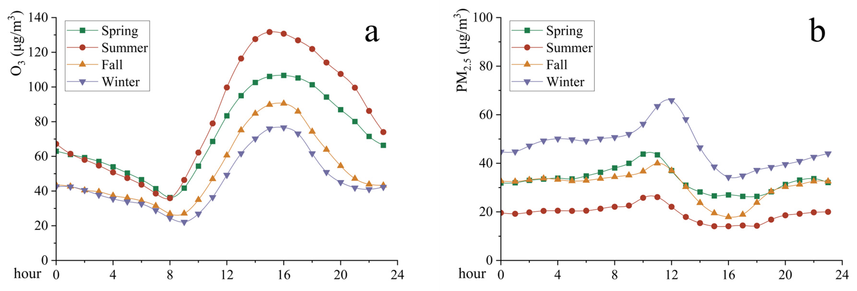
Xining was chosen to represent the overall pattern observed across Qinghai Province (Figure 3).
Overall, O3 peaks in summer and drops in winter, showing a clear afternoon maximum around 15:00–16:00 LT, driven by strong sunlight and higher boundary layers that favor photochemical production. In contrast, PM2.5 reaches its highest level in winter because of enhanced emissions and poor dispersion, while summer levels are the lowest. Its diurnal cycle shows morning and evening peaks, mainly due to traffic and stable nighttime conditions.

3.2. Local Attribution and Regression Model Performance

This section presents the results of MLR and GAM analyses to quantify the influence of meteorological and local emission-related factors on PM2.5 and O3 across Qinghai Province.

3.2.1. Linear Attribution with MLR

For each pollutant (PM2.5 and O3), three regression configurations were established as described in Section 2.2: a meteorological model (list (a) under Equation (1), rh, blh, ssrd, t2m, tp, wind), a pollutant model (list (b) under Equation (1), SO2, NO2, CO, PM10), and a combined model (list (c) under Equation (1)) including both groups. These configurations allow comparison of explanatory power and significance among different predictors.
Among all prefectures, Xining showed the best model performance with closely matched R2 and adjusted R2 values, indicating good robustness. It was therefore selected as the representative site, while results for other regions are summarized in Table A1.
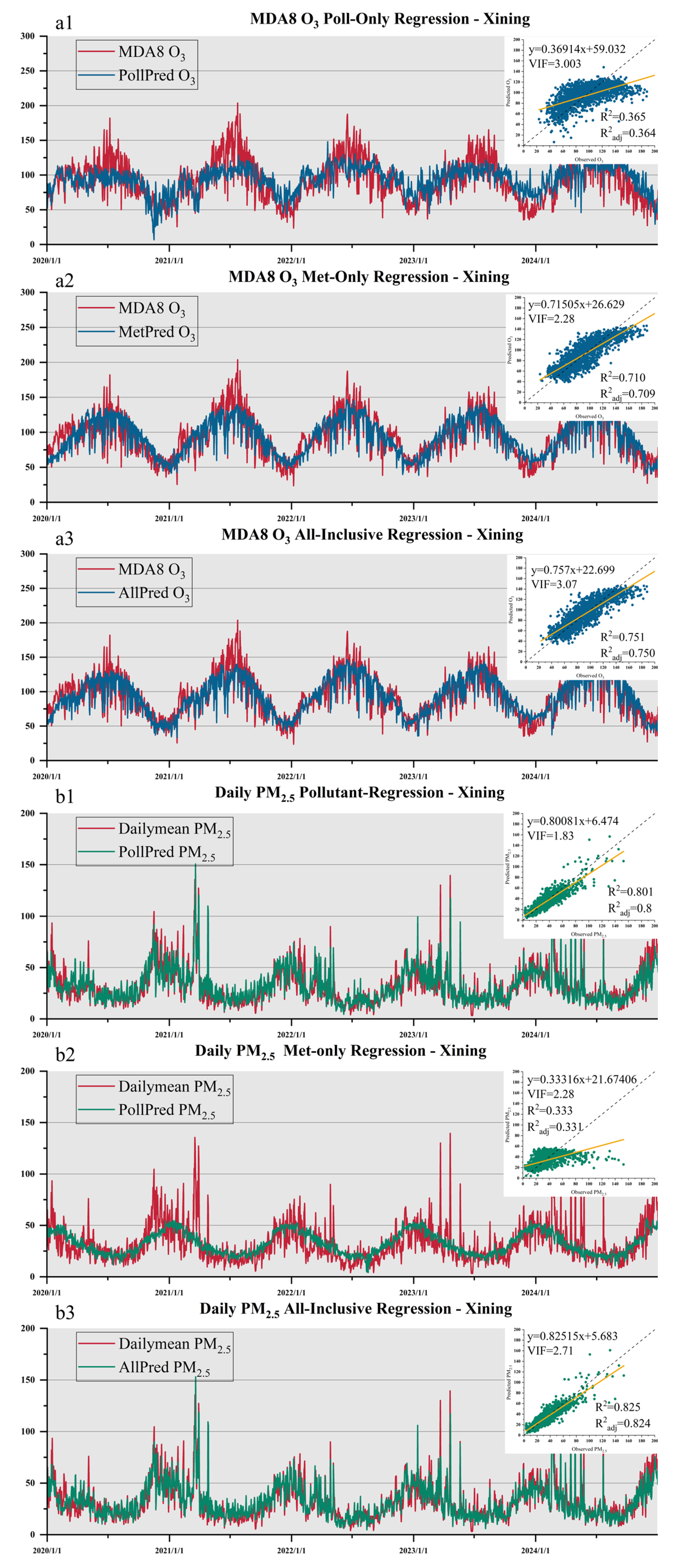
In Xining, the observed and modeled daily concentrations of O3 and PM2.5 during 2020–2024 were analyzed using three MLR configurations (Figure 4). Results for the remaining cities are provided in Appendix A Table A1. Those considering only meteorological factors, only pollutant factors, and a combination of both factors. The analysis revealed that the model considering only pollutant factors accounted for 80.1% of the variability in PM2.5 concentrations but only 36.5% for O3. Conversely, the meteorological-factor model explained 71.0% of the variability in O3 concentrations but a mere 33.3% for PM2.5. When the models integrated both meteorological and pollutant factors, there was a significant enhancement in explanatory power, with R2 values increasing to 82.5% for PM2.5 and 75.1% for O3. These results underscore the importance of considering both meteorological conditions and local emissions concurrently to significantly augment the explanatory capacity for both pollutants. However, the predominant driving factors differ markedly: O3 is primarily influenced by meteorological conditions, whereas PM2.5 is more strongly linked to local emissions. This pattern aligns with established atmospheric chemical processes, where O3 formation is significantly dependent on photochemical reactions and is sensitive to factors such as temperature, radiation, and boundary layer dynamics. In contrast, the generation and accumulation of PM2.5 are mainly driven by primary emissions and local secondary transformations [55,56,57,58,59]. Accordingly, strategies for O3 control should focus on regional collaborative management and regulatory measures under adverse meteorological conditions to mitigate O3 formation and accumulation. Simultaneously, PM2.5 mitigation should prioritize comprehensive reductions in emissions from local pollution sources, with which it is closely associated.
Residual diagnostics supported the reliability of the regression models. The Jarque–Bera values were between 102 and 104 (p < 0.001), showing a slight departure from normality. The Durbin–Watson values were close to 1.0, indicating mild serial correlation that is common in daily observations. These results suggest that the residual patterns are reasonable and do not affect the interpretation of the regression results.
For both O3 and PM2.5, linear models tended to underestimate observed concentrations during high-pollution episodes. The bias was more evident for O3, where all model types failed to reproduce peak values. For PM2.5, the pollutant- and combined-factor models performed slightly better, though underestimation still occurred. These results indicate that linear models cannot fully capture extreme events, implying that nonlinear processes and regional transport likely contribute to such peaks [60,61,62,63].
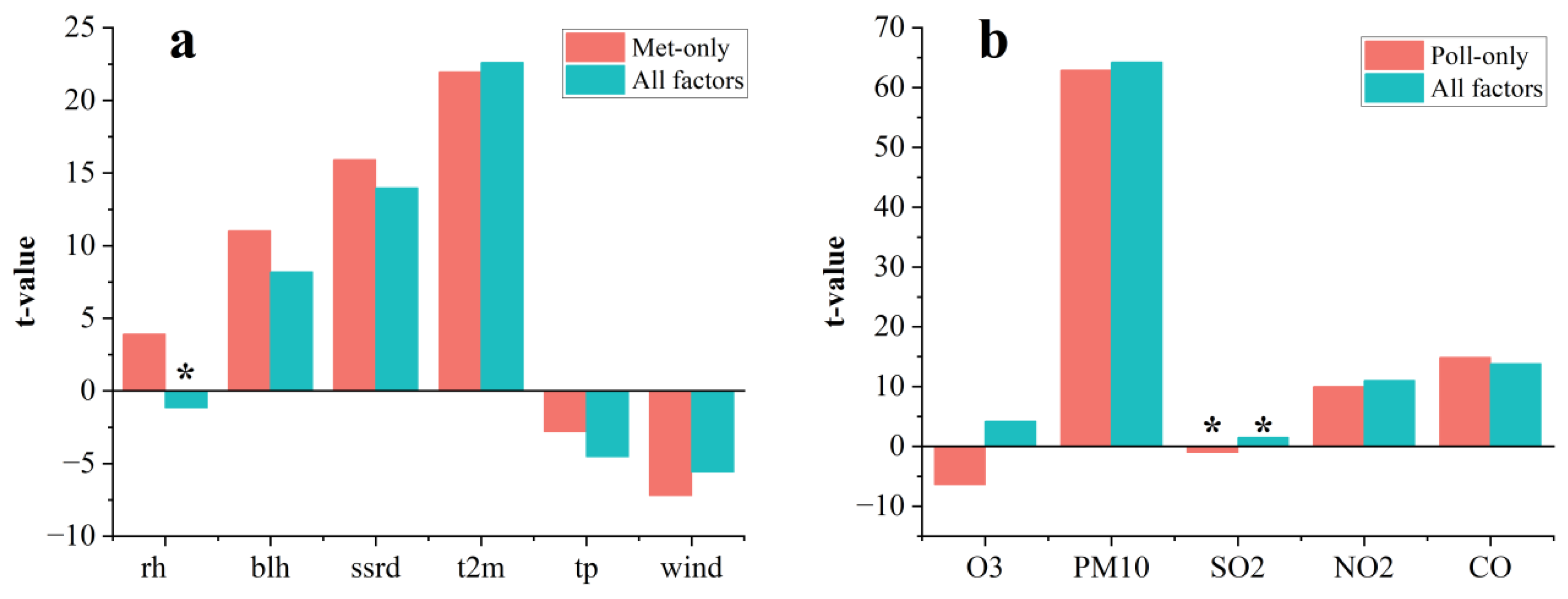
At the Xining site, t-statistics from the MLR models show that for O3, air temperature had the strongest effect, followed by solar radiation and boundary layer height. Wind speed and precipitation had negative effects, while relative humidity was not significant when pollutant factors were included. For PM2.5, PM10 showed the highest t-value, with NO2 and CO also contributing positively. SO2 had little influence. The addition of meteorological factors strengthened the role of O3, highlighting the strong impact of weather on PM2.5-O3 interactions. These nonlinear relationships justify further analysis with the GAM model (Figure 5).
The air quality monitoring sites in Qinghai Province display marked differences in elevation due to topographic and geographic variations. These elevation differences not only affect regional meteorological conditions and pollutant transport mechanisms but also contribute to the spatial heterogeneity in the goodness of fit (R2) of the multiple linear regression models for both O3 and PM2.5.
The monitoring sites in Qinghai Province present substantial elevation disparities, as shown in Table 2, with elevations ranging from 2072 m in Haidong to 2204 m in Xining, and reaching up to 3689 m in Yushu and 3718 m in Guoluo.
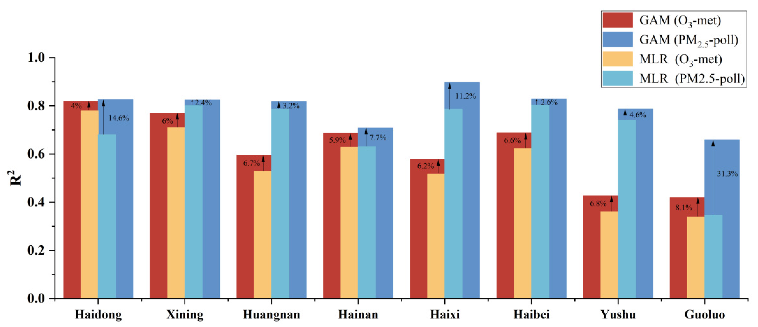
For both pollutants, R2 values decreased with increasing altitude (Figure 6). Low-altitude sites, such as Xining and Haidong, exhibited higher R2 values. In contrast, high-altitude sites, like Yushu and Guoluo, showed lower performance. This can be attributed to complex meteorological conditions at higher elevations. These include low air pressure, strong radiation, and high winds. Additionally, stronger external transport influences reduce the explanatory power of local factors [64,65]. The local-only model produced lower R2 values, indicating that local emissions alone cannot fully explain the variability of these pollutants. Correlation analysis further confirmed that model performance for both O3 and PM2.5 declined with elevation. The relationship for O3 was stronger (r = −0.91, p = 0.002), while for PM2.5, a moderate negative correlation was found (r = −0.51, p = 0.20). These results reflect the influence of local emission variability.

3.2.2. Nonlinear Supplementation with GAM

To overcome the constraints of linear models in adequately capturing nonlinear and threshold effects, GAM were implemented within the framework of MLR in regions demonstrating relatively high goodness of fit (Figure 7). This was done to delineate the nonlinear dynamics influencing the concentrations of O3 and PM2.5.
Across all sites, GAM models improved R2 by 10.8% for O3 and 17.4% for PM2.5 compared with MLR, showing stronger explanatory power. The improvement was about 5–15% in Yushu and Haixi and over 30% for PM2.5 in Guoluo. However, O3 models in high-altitude areas such as Yushu and Guoluo still performed poorly, suggesting that local factors alone cannot explain pollution there and that external transport likely plays a greater role. Based on these results, partial dependence plots were created for key variables at Xining to explore their nonlinear effects.
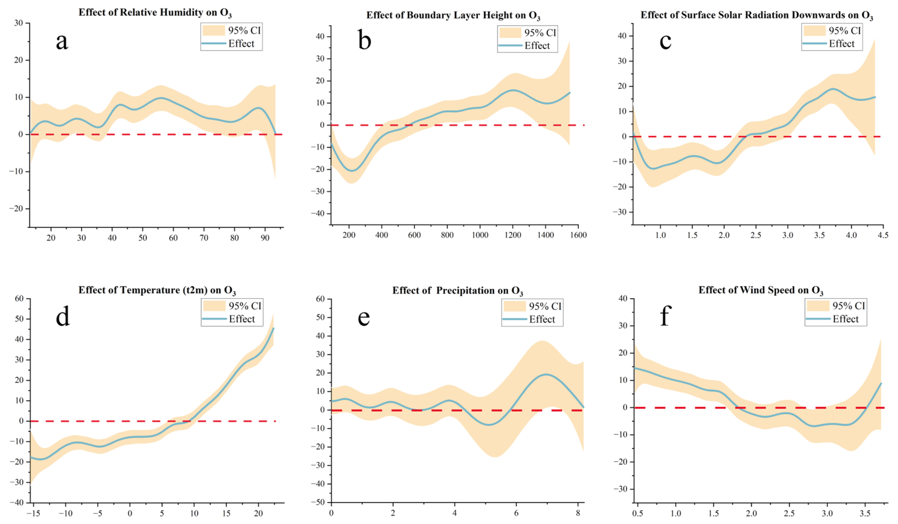
Air temperature (t2m), solar radiation (ssrd), and boundary layer height (blh) were identified as key meteorological factors influencing O3. GAM analysis (Figure 8) shows that O3 increases steadily with temperature, with a sharp rise above about 10 °C, confirming the strong temperature sensitivity of photochemical formation, consistent with findings in North China and the Yangtze River Delta [66,67]. Solar radiation and boundary layer height also show positive effects, enhancing O3 production and vertical mixing. In contrast, precipitation and wind speed exhibit threshold effects: when they exceed certain levels, O3 decreases markedly due to dilution and scavenging [68,69]. The nonlinear effect of relative humidity is weak, indicating limited independent influence and stronger interactions with other factors.
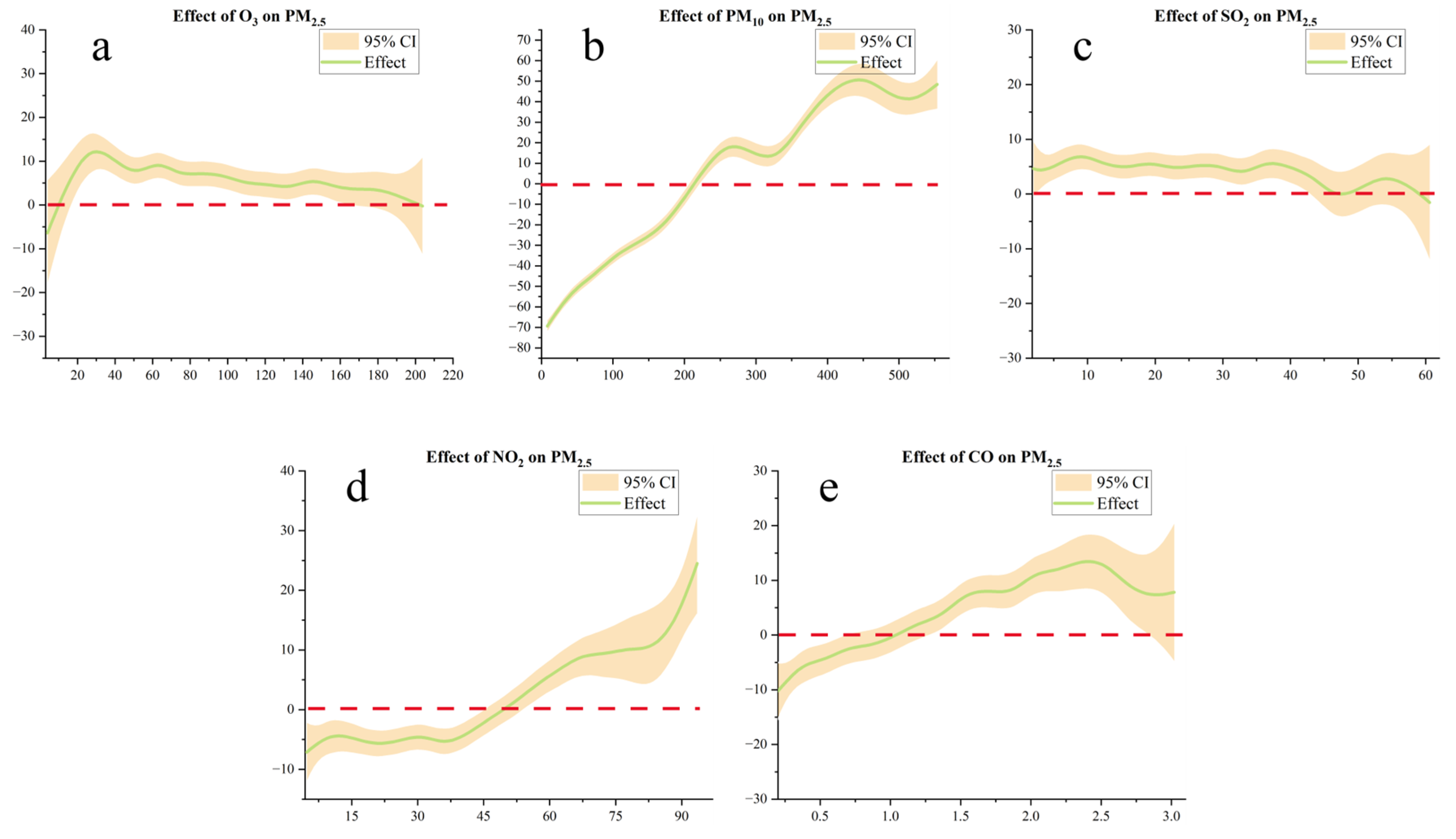
Figure 9 shows the partial dependence of PM2.5 on major pollutant factors. PM10 has the strongest positive effect, increasing steadily across all concentrations and sharply at higher levels, suggesting common sources such as dust and coal combustion, consistent with previous studies [70]. CO also shows a clear positive relationship, with PM2.5 rising rapidly when CO exceeds about 1.5 mg/m3, reflecting the combined influence of traffic and combustion emissions [71]. NO2 has little effect at low concentrations but increases PM2.5 sharply above about 45 µg/m3, indicating its role in secondary particle formation [72,73]. In contrast, SO2 shows only weak variation, implying a minor contribution to PM2.5 in this region.
Compared with MLR, the GAM model better captures the nonlinear responses of key factors, reducing the limitations of linear methods. However, in remote plateau regions such as Guoluo and Yushu, its explanatory power remains low, even with GAM, indicating that local factors alone cannot explain pollutant variations. This underscores the importance of external transport in high-altitude pollution episodes and provides a basis for subsequent trajectory analysis. Therefore, at lower altitudes, where the explanatory power of local factors is higher, controlling PM2.5 should emphasize emission reductions from industrial and transportation sources, whereas O3 management should strengthen regional coordination and meteorological forecasting.

3.3. External Transport Analysis

Building on the aforementioned premises, this section employs the HYSPLIT model to perform 72 h backward trajectory simulations for high-pollution and high-residual days. The simulations are combined with clustering analysis to identify key transport pathways and potential source regions. Quantitatively, the calculated external-transport intensity ( I e x t ) values ranged from 0.16–0.31 in low-altitude regions and 0.27–0.44 in high-altitude regions (Guoluo, Yushu). This indicates that external transport contributes approximately 20–40% of the observed pollution, with a particularly strong influence at higher elevations where local explanatory power is weakest.

3.3.1. Trajectory Simulation, Clustering, and Source Pathway Analysis for Low-R2 Sites/Days

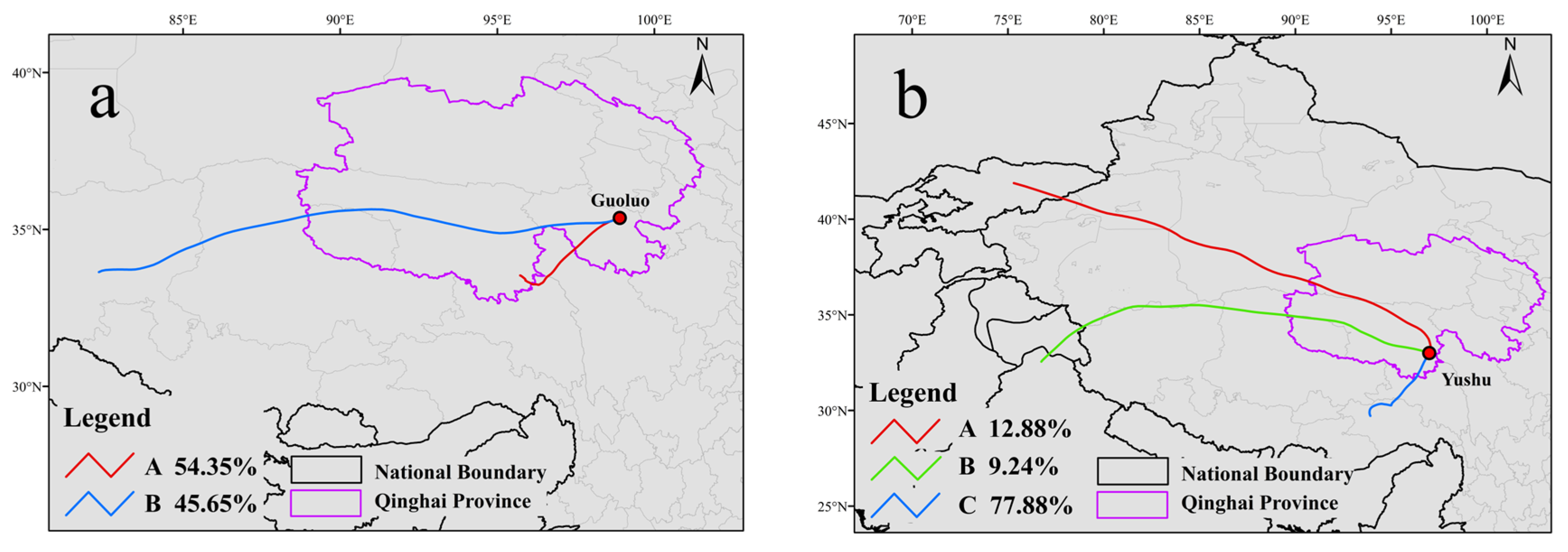
A total of 92, 22, and 165 high-pollution and high-residual days were identified for O3 (Guoluo), PM2.5 (Guoluo), and O3 (Yushu), respectively, generating 1028 trajectories for O3 and 264 for PM2.5. The optimal cluster numbers, determined by the Davies–Bouldin Index, were k = 2 for O3 in Guoluo, k = 3 for O3 in Yushu, and k = 2–3 for PM2.5 at different altitudes. These trajectories were then grouped using SOM clustering, and representative transport pathways with their relative proportions were extracted for subsequent analysis (Figure 10 and Figure 11).
In Guoluo, air masses mainly arrived from the southwest and west, indicating both local inflow and long-range transport across regions. In Yushu, transport was dominated by short-range circulation from the southwest, with occasional inflow from the northwest and west, reflecting combined local and regional influences.
In Guoluo, PM2.5 transport showed multiple pathways that varied with altitude. At lower levels (500 m), air masses mainly arrived from the southwest and west, reflecting local and near-regional influences. At 1000 m and above, trajectories increasingly originated from the west and northwest, indicating enhanced long-range transport. Overall, higher altitudes were dominated by cross-regional inputs, whereas local sources played a greater role near the surface.
To assess the validity of the clustering results, the Kruskal–Wallis H test was employed to compare pollutant concentrations across different trajectory categories. The findings indicated statistically significant differences in concentrations among categories (p < 0.001), confirming that the clustering technique effectively differentiated between transport pathways associated with varying levels of pollution.

3.3.2. Spatial Identification of Potential Source Regions by WCWT

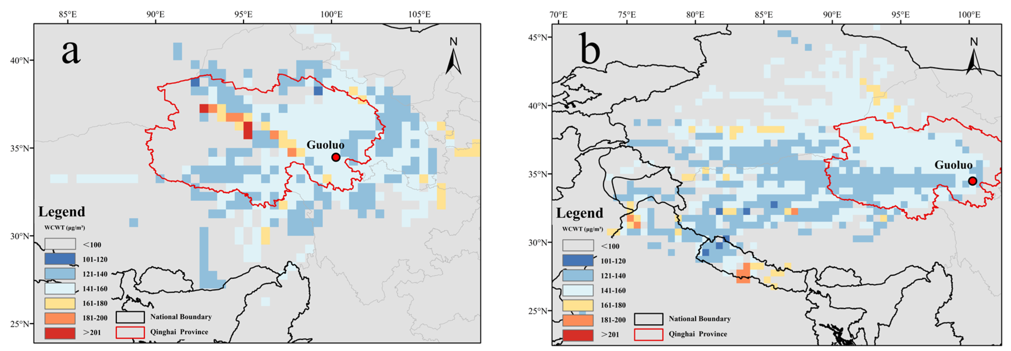
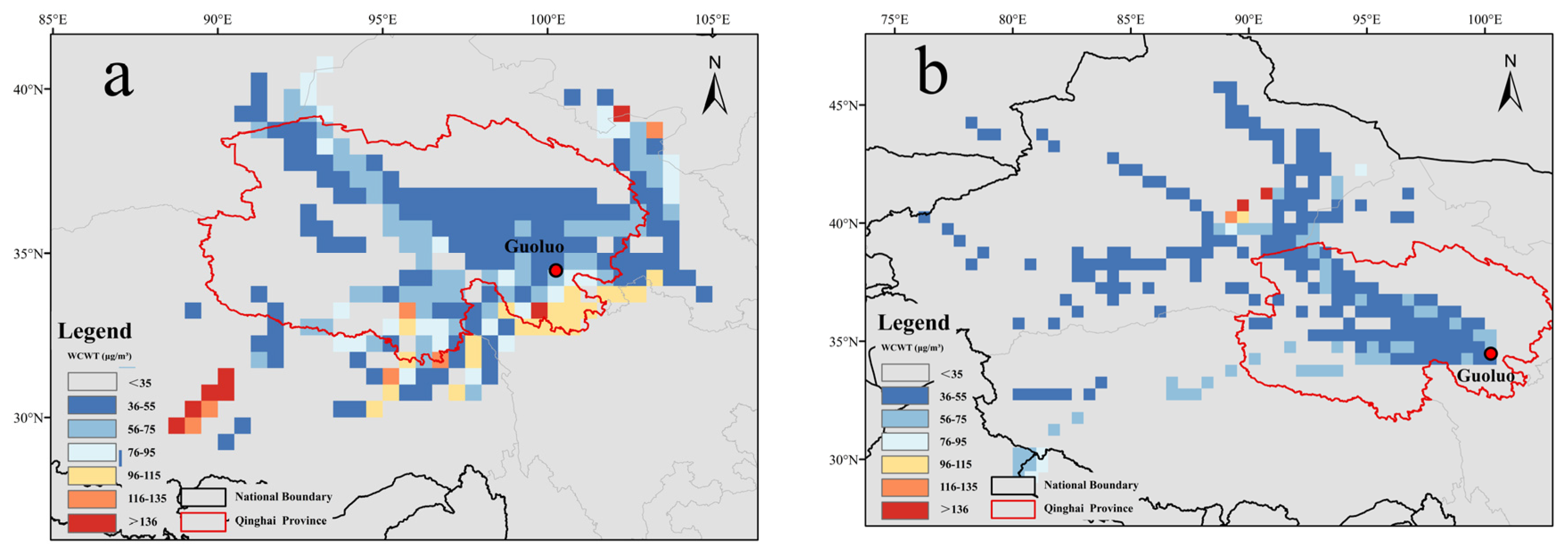
Building on the trajectory findings from high-pollution, high-residual days discussed in Section 3.2.1, WCWT calculations were performed for each trajectory category to delineate the spatial distribution of potential source regions and their respective contributions to different transport pathways. The results, detailed in Figure 12, Figure 13, Figure 14, Figure 15 and Figure 16, illustrate the distribution patterns for each category.
It should be noted that in certain regions or pollutants, the high-value areas identified by WCWT may not exactly coincide with the dominant transport directions obtained from SOM clustering. This discrepancy arises from their methodological focus: SOM emphasizes airflow pathways, while WCWT identifies potential source regions where pollutants may accumulate along the trajectories. The two approaches are therefore complementary in interpreting transport dynamics.
At 500 m in Guoluo, O3 transport was mainly driven by local and nearby regional sources from the southwest and west. High-contribution areas within and north of Guoluo reached over 200 μg/m3, while concentrations decreased eastward and southeastward with increasing transport distance. Cluster A showed a maximum WCWT value of 226.88 μg/m3 and an average of 145.33 μg/m3, indicating strong local and medium-range influence. In contrast, Cluster B exhibited lower overall contributions, with most areas below 140 μg/m3 and moderate values of 160–200 μg/m3 along the western and southern edges of the Plateau. The maximum and mean values were 196.25 μg/m3 and 142.77 μg/m3, suggesting long-range transport with progressive dilution of pollutants.
At 500 m in Yushu, WCWT analysis of O3 trajectories during high-pollution, high-residual days shows distinct spatial patterns (Figure 13). Cluster A exhibits a high-contribution zone across southern and southeastern Yushu, where concentrations exceed 200 μg/m3, with a maximum of 168.08 μg/m3 and an average of 136.41 μg/m3. This distribution, aligned northwest–southeast along the southern Tibetan Plateau, indicates combined effects of nearby sources and transboundary transport. Cluster B shows generally low contributions, mostly below 120 μg/m3, with a few moderate areas (120–160 μg/m3) along the southern and western plateau margins. The maximum concentration is 160.0 μg/m3, suggesting long-range transport with pollutant dilution. Cluster C presents higher contributions to the east of Yushu and southeastern Qinghai, expanding westward, with a maximum of 189.88 μg/m3 and an average of 138.16 μg/m3. This pattern reflects the influence of both short- and medium-range transport on O3 accumulation.
A comparison of the WCWT results for O3 between Guoluo and Yushu shows clear differences in the location and strength of high-contribution areas. In Guoluo, high values are mainly concentrated in the southwest, reflecting both local and medium-range transport. This zone extends eastward into eastern Qinghai and the western Sichuan Plateau, where contributions quickly weaken. In contrast, Yushu’s high-value areas are linked to the southern border and the Qinghai–Tibet boundary, showing stronger and more continuous contributions across short- and medium-range transport. For Cluster B, Guoluo shows low and scattered values, suggesting stronger dilution during long-range transport, while Yushu keeps moderate contributions over southwestern Sichuan, indicating more persistent long-range effects. In Cluster C, Yushu forms a continuous mid-level belt stretching eastward, which is absent in Guoluo. These contrasts highlight the different source regions and transport pathways shaped by local geography and weather.
At 500 m in Guoluo, PM2.5 transport was mainly influenced by local and nearby regional sources. A pronounced high-contribution belt extended southeastward across Guoluo, with core values above 75 μg/m3 and peak areas exceeding 115 μg/m3. The maximum and average WCWT concentrations were 147.08 μg/m3 and 65.60 μg/m3, indicating strong local and medium-range effects. In contrast, Cluster B showed lower overall contributions, mostly below 75 μg/m3, with only a few discontinuous moderate patches. Its maximum and average values were 147.08 μg/m3 and 50.60 μg/m3, suggesting weak long-range influence.
At 1000 m, the influence range broadened and long-distance effects became more evident. Cluster A formed a continuous medium-concentration belt from Guoluo to eastern Qinghai, with localized peaks over 95 μg/m3 (max 111.83 μg/m3, avg 48.74 μg/m3). Cluster B followed a west–east corridor dominated by values below 75 μg/m3, while Cluster C extended southwestward with concentrations surpassing 135 μg/m3 (max 147.08 μg/m3, avg 61.06 μg/m3), reflecting increasing regional and cross-border transport contributions.
At 1500 m, the transport range expanded further, but contribution levels declined. Cluster A showed scattered low-value cells (mostly <55 μg/m3; max 61.08 μg/m3, avg 46.69 μg/m3), indicating weak regional transport. Cluster B formed a westerly transport belt with occasional peaks up to 135 μg/m3 (max 147.08 μg/m3, avg 62.90 μg/m3), suggesting diluted long-range inputs. Cluster C, mainly over Qinghai and adjacent regions, displayed generally low concentrations (<65 μg/m3; max 71.68 μg/m3, avg 44.78 μg/m3).
Overall, at 500 m the transport was dominated by concentrated local and medium-range sources, while at 1000 m the signals from distant sources strengthened along continuous corridors. At 1500 m, the spatial coverage widened but high-value areas became sparse. Despite differences in intensity, the main transport pathways remained consistent across heights, confirming the robustness of PM2.5 transport patterns and the progressive dilution of pollutants with altitude.

3.3.3. Case Study of Extreme Pollution Episodes and External Transport Characteristics

To elucidate further the role of external transport in the development of extreme pollution events, this section examines a PM2.5 extreme event in Guoluo on 28 February 2021, and an O3 extreme event in Yushu on 1 June 2024. Backward trajectory simulations are employed to reveal the external transport characteristics associated with these pollution events.
  • Guoluo PM2.5 Pollution Episode (28 February 2021)
On 28 February 2021, Guoluo experienced a severe particulate pollution event. The PM2.5 concentration reached 147.1 μg/m3, while PM10 peaked at 468.1 μg/m3, giving a PM10/PM2.5 ratio of about 3.2. This high ratio (coarse fraction ≈ 68.6%) suggests that dust made a dominant contribution. The MLR model predicted a PM2.5 concentration of 73.31 μg/m3, which is roughly half of the observed value. This indicates that local sources alone could not explain the pollution. The remaining ≈50% (≈73.8 μg/m3) likely came from external transport, representing about a twofold increase over the local baseline. The 72 h backward trajectories (Figure 17) showed that air masses at 500–1000 m mainly came from the Qaidam Basin and the Hexi Corridor, while those at 1500 m extended southwestward. This pattern reveals a multi-level inflow of dust. Together with the WCWT results, these findings confirm that about half of the PM2.5 originated from long-range dust transport, while poor dispersion conditions acted as a secondary factor.
2.
Yushu O3 Pollution Episode (1 June 2024)
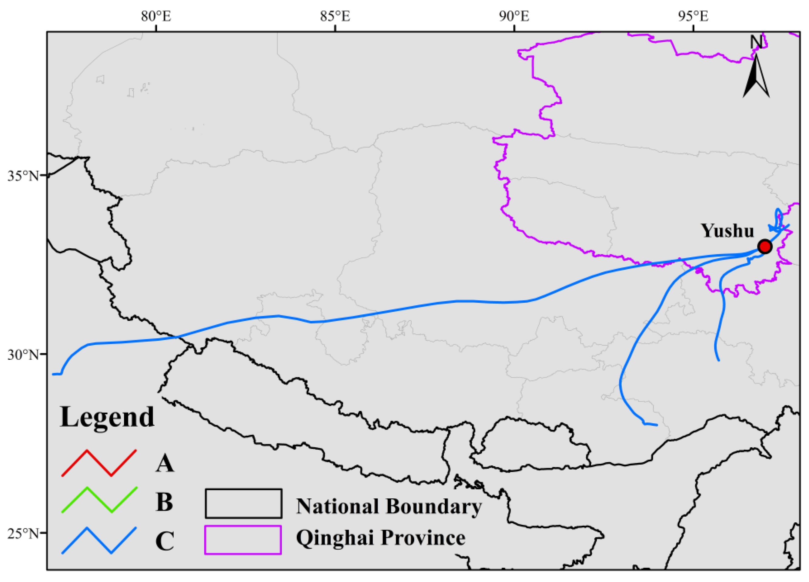
On 1 June 2024, Yushu experienced a notable O3 pollution episode, with the MDA8 O3 concentration reaching 189.9 μg/m3. The day was marked by poor atmospheric ventilation, high relative humidity, and precipitation, while precursor levels remained low. The MLR model predicted only 90.77 μg/m3, less than half of the observed value, indicating that local photochemical processes alone could not explain the peak. The remaining ≈52% (≈99 μg/m3) can be attributed to external transport. The 72 h backward trajectories (Figure 18, at 500 m) showed that air masses over Yushu mainly originated from the southwest and west, extending toward South Asia. This pattern reveals strong external influence on local air quality. Together with the WCWT results, these findings confirm that long-range transport was the dominant driver of this O3 episode, while unfavorable local dispersion acted as a secondary amplifying factor.

3.4. Integrated Discussion

The present study revealed a clear altitude-dependent pattern in the pollution mechanisms over the Tibetan Plateau, driven by both local and transboundary processes. This finding is consistent with previous observations of elevation-related gradients in northwestern China and the central Plateau [74,75,76]. At lower altitudes, both PM2.5 and O3 are mainly controlled by local factors. PM2.5 is influenced by anthropogenic emissions and frequent winter inversions, while O3 is affected by local meteorological conditions such as temperature, solar radiation, and boundary-layer height. These results are in line with previous studies in Xining and Lanzhou, where seasonal variations of PM2.5 and O3 were largely determined by local emissions and weather conditions [77,78,79]. At higher elevations, the influence of local factors becomes weaker, and stronger westerly winds promote long-range transport of dust and precursors. This agrees with trajectory and modeling studies that identified dominant westerly and South Asian inflows over the Plateau [80,81]. However, this study further shows a clearer altitude threshold above which local effects decline and external transport becomes dominant. Overall, these features distinguish the Plateau from lowland basins, where human emissions remain the main driver of pollution throughout the year, and highlight the combined effects of meteorological, topographic, and chemical processes on air pollution formation.
Building upon these findings, several limitations and future directions should be noted. While the observational period covers only five years (2020–2024), it ensures consistent data across all sites and captures multiple seasonal cycles. Similar time spans have been used in previous studies [82,83,84,85], but we acknowledge that longer datasets would better reflect interannual variability and will be considered in future work. First, the relatively short observational period and the absence of certain precursor species may have constrained the comprehensiveness of the results. Second, although MLR and GAM provided valuable insights into the relationships between local factors and pollutant concentrations, these statistical models remain inadequate for fully capturing the complex non-linear chemical processes underlying atmospheric pollution. Third, the reliability of the HYSPLIT and WCWT analyses is highly dependent on the accuracy of meteorological inputs and the sample size, which introduces uncertainties, particularly under extreme conditions [86,87,88]. In addition, the use of ERA5 reanalysis data introduces uncertainties over the complex terrain of the Tibetan Plateau. ERA5 tends to overestimate rainfall frequency and duration over the eastern margin [89] and shows a wet bias of about 20–30% in western China [90]. It also underestimates near-surface temperature by 1–2 °C in the Qilian Mountains [91], overestimates shortwave radiation by around 15 W m−2 [92], and underestimates wind speed in high-altitude areas [93]. These biases suggest that the overall uncertainty of ERA5 meteorological forcing over the Plateau is roughly within ±20–40%, which may slightly affect this study’s results. Future work will use higher-resolution or bias-corrected datasets to improve model reliability. Finally, the current analysis qualitatively assessed the balance between local influences and external transport without explicitly quantifying their respective contributions. Future research should aim to refine this framework by incorporating regression coefficient or residual decomposition methods to achieve more robust quantification, and by coupling with three-dimensional chemical transport models (e.g., WRF-Chem, GEOS-Chem) to simulate chemical mechanisms with greater fidelity [94,95,96]. In addition, integrating high-resolution remote sensing products and multi-source datasets may further enhance the attribution of pollution dynamics on the Plateau and extend the applicability of the framework to other complex regions.

4. Conclusions

This study combined multivariate statistical modeling with trajectory analysis to build an integrated MRG–HSW framework for identifying the drivers of PM2.5 and O3 pollution across eight prefectures in Qinghai Province. In low-altitude areas, PM2.5 was mainly affected by local human activities (R2 = 0.63–0.80), while O3 responded more strongly to meteorological conditions (R2 = 0.53–0.78). O3 increased with temperature, solar radiation, and boundary layer height but decreased with precipitation and wind speed. PM2.5 was mainly influenced by PM10, CO, and NO2, with SO2 having a minor effect. At high altitudes, the explanatory power of local factors dropped sharply (R2 = 0.34–0.36), indicating that local processes alone could not explain pollution peaks. External transport thus became the main driver. Quantitative results show that the external-transport intensity ( I e x t ) ranged from 0.16–0.31 in low-altitude regions and 0.27–0.44 in high-altitude regions, meaning that external inflow contributed about 20–40% of the total pollution and had a stronger impact in higher areas. In Guoluo, long-range dust from the Qaidam Basin and Hexi Corridor added to PM2.5, while O3 was affected by both short-range inflow from the southeast and long-range transport from the west. In Yushu, O3 was influenced mainly by air masses from the northwest and South Asia. These results confirm that the spatial differences of PM2.5 and O3 on the Tibetan Plateau arise from both local emission–meteorology interactions and large-scale external transport.
Collectively, this study deepens the understanding of pollution formation mechanisms on the Tibetan Plateau and provides evidence for differentiated regional management and cross-regional cooperation. In lower-altitude areas, PM2.5 mitigation should prioritize reducing local emissions, particularly from industrial and vehicular sources, while O3 control should focus on meteorological influences and coordinated regional actions. In higher-altitude prefectures, where external transport plays a dominant role, collaboration with neighboring provinces and transboundary partners such as South Asia is essential. These differentiated strategies contribute directly to sustainable air quality governance by aligning local mitigation efforts with regional atmospheric circulation patterns. Integrating the results into long-term planning-such as the optimization of energy and transportation structures, early warning networks, and regional emission-trading mechanisms-can help achieve both pollution control and carbon reduction co-benefits. The MRG-HSW framework provides a transferable and science-based decision-support tool for evidence-driven policymaking, facilitating adaptive and cooperative air quality management in the ecologically sensitive Plateau region.

Author Contributions

Conceptualization, Y.L. and Y.H.; methodology, Y.L.; software, Y.L.; validation, Y.L., Y.H., and Y.W.; formal analysis, Y.L.; investigation, Y.L. and H.N.; resources, G.L., X.Z., Y.Z., and L.W.; data curation, Y.L.; writing—original draft preparation, Y.L.; writing—review and editing, Y.H. and Y.W.; visualization, Y.L.; supervision, Y.H.; project administration, Y.H.; funding acquisition, Y.H. All authors have read and agreed to the published version of the manuscript.

Funding

This research was funded by the Qinghai Provincial Eco-Environmental Planning and Environmental Protection Technology Center through the “Qinghai Province Air Pollution Status Assessment and Refined Management Support Project” (grant number YG-2023-03-H).

Institutional Review Board Statement

Not applicable.

Informed Consent Statement

Not applicable.

Data Availability Statement

These data were derived from the following resources available in the public domain: The air quality data utilized in this study are publicly available from the China National Environmental Monitoring Center (CNEMC) at http://www.cnemc.cn. The ERA5 reanalysis meteorological data are accessible from the Copernicus Climate Data Store (CDS) at https://cds.climate.copernicus.eu (accessed on 1 June 2025). The GDAS1 meteorological fields can be obtained from the NOAA Air Resources Laboratory (ARL) at https://www.ready.noaa.gov/gdas1.php (accessed on 1 June 2025). The model outputs generated in this study are available from the corresponding author upon reasonable request.

Acknowledgments

The authors extend their gratitude to Flaticon (https://www.flaticon.com) for providing the icons used in the graphical illustrations.

Conflicts of Interest

The authors declare no conflicts of interest. The funders did not influence the study design, data collection, analysis, interpretation, manuscript writing, or the decision to publish the results.

Abbreviations

The following abbreviations are used in this manuscript:
PM2.5Particulate matter with aerodynamic diameter less than 2.5 μm
O3Ozone
ERA5ECMWF Reanalysis v5
GDASGlobal Data Assimilation System
CNEMCChina National Environmental Monitoring Center
MRGMultiple Regression with residual-based screening and GAM
HSWHYSPLIT–SOM–WCWT trajectory-based framework

Appendix A

Table A1. Coefficient of determination (R2) of O3 and PM2.5 under different modeling scenarios in eight cities of Qinghai Province.
CityR2 (O3–Meteorology)R2 (O3–Pollutants)R2 (O3–All Factors)R2 (PM2.5–Meteorology)R2 (PM2.5–Pollutants)R2 (PM2.5–All Factors)
Haibei0.6230.0540.6330.0960.8030.822
Huangna0.5290.2930.5610.190.7860.805
Hainan0.6280.2050.6350.1130.6310.648
Guoluo0.3390.0250.3480.0680.3460.36
Yushu0.360.270.420.3940.7410.773
Haixi0.5170.170.5350.0240.7860.789
Haidong0.7790.3640.7990.2820.6810.728
Xining0.710.3650.7510.3330.8010.825

References

  1. Lyu, Y.; Wu, Z.; Wu, H.; Pang, X.; Qin, K.; Wang, B.; Ding, S.; Chen, D.; Chen, J. Tracking Long-Term Population Exposure Risks to PM2.5 and Ozone in Urban Agglomerations of China 2015–2021. Sci. Total Environ. 2023, 854, 158599. [Google Scholar] [CrossRef]
  2. Wang, B.; Ji, Y.; Yang, X.; Shi, J.; Xu, W.; Ma, J.; Shen, R.; Wang, B.; Zhang, J.; Feng, Y. Population Exposure Evaluation and Value Loss Analysis of PM2.5 and Ozone in China. J. Environ. Manag. 2025, 376, 124480. [Google Scholar] [CrossRef]
  3. Xiao, Q.; Geng, G.; Xue, T.; Liu, S.; Cai, C.; He, K.; Zhang, Q. Tracking PM2.5 and O3 Pollution and the Related Health Burden in China 2013–2020. Environ. Sci. Technol. 2022, 56, 6922–6932. [Google Scholar] [CrossRef]
  4. Zhang, X.; Cheng, C.; Zhao, H. A Health Impact and Economic Loss Assessment of O3 and PM2.5 Exposure in China from 2015 to 2020. GeoHealth 2022, 6, e2021GH000531. [Google Scholar] [CrossRef]
  5. Li, Y.; Wang, T.; Wang, Q.; Qu, Y.; Wu, H.; Xie, M.; Li, M.; Li, S.; Zhuang, B. Spatiotemporal Variations of PM2.5 and O3 Relationship during 2014–2021 in Eastern China. Aerosol Air Qual. Res. 2023, 23, 230060. [Google Scholar] [CrossRef]
  6. Ma, X.; Yin, Z.; Cao, B.; Wang, H. Meteorological Influences on Co-Occurrence of O3 and PM2.5 Pollution and Implication for Emission Reductions in Beijing-Tianjin-Hebei. Sci. China Earth Sci. 2023, 66, 1258–1267. [Google Scholar] [CrossRef] [PubMed]
  7. Ministry of Ecology and Environment of the People’s Republic of China. China Ecological and Environmental Status Bulletin; Ministry of Ecology and Environment: Beijing, China, 2024. [Google Scholar]
  8. Guan, Y.; Xiao, Y.; Wang, Y.; Zhang, N.; Chu, C. Assessing the Health Impacts Attributable to PM2.5 and Ozone Pollution in 338 Chinese Cities from 2015 to 2020. Environ. Pollut. 2021, 287, 117623. [Google Scholar] [CrossRef]
  9. Shao, T.; Wang, P.; Yu, W.; Gao, Y.; Zhu, S.; Zhang, Y.; Hu, D.; Zhang, B.; Zhang, H. Drivers of Alleviated PM2.5 and O3 Concentrations in China from 2013 to 2020. Resour. Conserv. Recycl. 2023, 197, 107110. [Google Scholar] [CrossRef]
  10. Wang, L.; Liu, B.; Li, R.; Chen, X.; Liu, L.; Tang, X.; Liu, J.; Liao, Z.; Xin, J.; Wang, Y.; et al. Prediction of Daily PM2.5 and Ozone Based on High-Density Weather Stations in China: Nonlinear Effects of Meteorology, Human and Ecosystem Health Risks. Atmos. Res. 2023, 293, 106889. [Google Scholar] [CrossRef]
  11. Xu, T.; Zhang, C.; Liu, C.; Hu, Q. Variability of PM2.5 and O3 Concentrations and Their Driving Forces over Chinese Megacities during 2018–2020. J. Environ. Sci. 2023, 124, 1–10. [Google Scholar] [CrossRef]
  12. Cheng, B.; Ma, Y.; Feng, F.; Zhang, Y.; Shen, J.; Wang, H.; Guo, Y.; Cheng, Y. Influence of Weather and Air Pollution on Concentration Change of PM2.5 Using a Generalized Additive Model and Gradient Boosting Machine. Atmos. Environ. 2021, 255, 118437. [Google Scholar] [CrossRef]
  13. Hou, Y.; Wang, Q.; Tan, T. Evaluating Drivers of PM2.5 Air Pollution at Urban Scales Using Interpretable Machine Learning. Waste Manag. 2025, 192, 114–124. [Google Scholar] [CrossRef] [PubMed]
  14. Wei, Q.; Chen, Y.; Zhang, H.; Jia, Z.; Yang, J.; Niu, B. Simulation and Prediction of PM2.5 Concentrations and Analysis of Driving Factors Using Interpretable Tree-Based Models in Shanghai, China. Environ. Res. 2025, 270, 121003. [Google Scholar] [CrossRef] [PubMed]
  15. Duan, W.; Wang, X.; Cheng, S.; Wang, R.; Zhu, J. Influencing Factors of PM2.5 and O3 from 2016 to 2020 Based on DLNM and WRF-CMAQ. Environ. Pollut. 2021, 285, 117512. [Google Scholar] [CrossRef]
  16. Ma, X.; Liu, H.; Peng, Z. Improving WRF-Chem PM2.5 Predictions by Combining Data Assimilation and Deep-Learning-Based Bias Correction. Environ. Int. 2025, 195, 109199. [Google Scholar] [CrossRef]
  17. Väisänen, O.; Hao, L.; Virtanen, A.; Romakkaniemi, S. Trajectory-Based Analysis on the Source Areas and Transportation Pathways of Atmospheric Particulate Matter over Eastern Finland. Tellus B Chem. Phys. Meteorol. 2020, 72, 1799687. [Google Scholar] [CrossRef]
  18. Li, H.; He, Q.; Liu, X. Identification of Long-Range Transport Pathways and Potential Source Regions of PM2.5 and PM10 at Akedala Station, Central Asia. Atmosphere 2020, 11, 1183. [Google Scholar] [CrossRef]
  19. Gao, A.; Gao, B.; Li, S.; Yao, W.; Sun, W.; Cao, X.; Liu, Y.; Zhang, H.; Zhang, B. Pollution Characteristics, Potential Source Areas, and Transport Pathways of PM2.5 and O3 in an Inland City of Shijiazhuang, China. Air Qual. Atmos. Health 2024, 17, 1307–1323. [Google Scholar] [CrossRef]
  20. Cui, L.; Song, X.; Zhong, G. Comparative Analysis of Three Methods for HYSPLIT Atmospheric Trajectories Clustering. Atmosphere 2021, 12, 698. [Google Scholar] [CrossRef]
  21. Mulyana, M.R.; Aristiawan, Y.; Linggabinangkit, C.; Samodro, R.A.; Prasetia, H.; Fauziyyah, N.; Iswara, N.J.P.; Ega, A.V.; Prihhapso, Y. Urban Air Pollutant Mapping and Tracing Using Mobile In-Situ Measurements Combined with Clustering and Trajectory Analysis. Environ. Monit. Assess. 2025, 197, 1–14. [Google Scholar] [CrossRef]
  22. Nirwan; Siddiqui, A.; Shaeb, H.B.; Chauhan, P.; Singh, R.P. Gaseous Air Pollutants and Its Association with Stubble Burning: An Integrated Approach Using Ground and Satellite Based Datasets and Concentration Weighted Trajectory (CWT) Analysis. Res. Sq. 2023. published. [Google Scholar] [CrossRef]
  23. Chham, E.; Orza, J.A.G. Evaluating the Impact of the Aerosol Sampling Time Interval on CWT and PSCF Source-Receptor Models: A Critical Perspective. Sci. Total Environ. 2025, 971, 179069. [Google Scholar] [CrossRef]
  24. Lu, N.; Zhang, L.; Wang, X.; Liu, Z.; Li, D.; Xu, J.; Tan, H.; Zhou, M.; Henze, D.K. Assessing the Nonlinearity of Wintertime PM2.5 Formation in Response to Precursor Emission Changes in North China with the Adjoint Method. Environ. Res. Lett. 2024, 19, 084048. [Google Scholar] [CrossRef]
  25. Ge, S.; Wang, S.; Xu, Q.; Ho, T. Source Apportionment Simulations of Ground-Level Ozone in Southeast Texas Employing OSAT/APCA in CAMx. Atmos. Environ. 2021, 253, 118370. [Google Scholar] [CrossRef]
  26. Irankunda, E.; Török, Z. Monitoring and Dispersion Modelling of Particulate Matter (PM2.5) in Rwanda. Aerosol Sci. Eng. 2025. published. [Google Scholar] [CrossRef]
  27. Kim, K.-C.; Song, H.-J.; Lee, C.-S.; Lim, Y.-J.; Ahn, J.-Y.; Seo, S.-J.; Han, J.-S. Characteristics and Source Identification for PM2.5 Using PMF Model: Comparison of Seoul Metropolitan Area with Baengnyeong Island. Atmosphere 2024, 15, 1146. [Google Scholar] [CrossRef]
  28. Guttikunda, S.K.; Nishadh, K.A.; Gota, S.; Singh, P.; Chanda, A.; Jawahar, P.; Asundi, J. Air Quality, Emissions, and Source Contributions Analysis for the Greater Bengaluru Region of India. Atmos. Pollut. Res. 2019, 10, 941–953. [Google Scholar] [CrossRef]
  29. Liu, F.; Van Der, A.R.J.; Eskes, H.; Ding, J.; Mijling, B. Evaluation of Modeling NO2 Concentrations Driven by Satellite-Derived and Bottom-up Emission Inventories Using in Situ Measurements over China. Atmos. Chem. Phys. 2018, 18, 4171–4186. [Google Scholar] [CrossRef]
  30. Ozkurt, N.; Sari, D.; Akalin, N.; Hilmioglu, B. Evaluation of the Impact of SO2 and NO2 Emissions on the Ambient Air-Quality in the Çan–Bayramiç Region of Northwest Turkey during 2007–2008. Sci. Total Environ. 2013, 456–457, 254–266. [Google Scholar] [CrossRef] [PubMed]
  31. He, H.; Vinnikov, K.Y.; Li, C.; Krotkov, N.A.; Jongeward, A.R.; Li, Z.; Stehr, J.W.; Hains, J.C.; Dickerson, R.R. Response of SO2 and Particulate Air Pollution to Local and Regional Emission Controls: A Case Study in Maryland. Earth’s Future 2016, 4, 94–109. [Google Scholar] [CrossRef]
  32. Mallik, C.; Ghosh, D.; Ghosh, D.; Sarkar, U.; Lal, S.; Venkataramani, S. Variability of SO2, CO, and Light Hydrocarbons over a Megacity in Eastern India: Effects of Emissions and Transport. Environ. Sci. Pollut. Res. 2014, 21, 8692–8706. [Google Scholar] [CrossRef]
  33. Li, H.; Chen, R.; Han, C.; Yang, Y. Evaluation of the Spatial and Temporal Variations of Condensation and Desublimation over the Qinghai–Tibet Plateau Based on Penman Model Using Hourly ERA5-Land and ERA5 Reanalysis Datasets. Remote Sens. 2022, 14, 5815. [Google Scholar] [CrossRef]
  34. Yin, B.; Xie, Y.; Yao, C.; Liu, B.; Liu, B. Evaluating Rainfall Erosivity on the Tibetan Plateau by Integrating High Spatiotemporal Resolution Gridded Precipitation and Gauge Data. Sci. Total Environ. 2024, 947, 174334. [Google Scholar] [CrossRef] [PubMed]
  35. Zhang, Q.; Li, J. Multi-Scale Assessment of ERA5 Hourly Pressure-Level Data on a Global Scale with in-Situ Observations. Theor. Appl. Clim. 2025, 156, 575. [Google Scholar] [CrossRef]
  36. Valentini, M.; Dos Santos, G.B.; Muller Vieira, B. Multiple Linear Regression Analysis (MLR) Applied for Modeling a New WQI Equation for Monitoring the Water Quality of Mirim Lagoon, in the State of Rio Grande Do Sul—Brazil. SN Appl. Sci. 2021, 3, 70. [Google Scholar] [CrossRef]
  37. Shams, S.R.; Jahani, A.; Kalantary, S.; Moeinaddini, M.; Khorasani, N. The Evaluation on Artificial Neural Networks (ANN) and Multiple Linear Regressions (MLR) Models for Predicting SO2 Concentration. Urban Clim. 2021, 37, 100837. [Google Scholar] [CrossRef]
  38. Xie, Y.; Zhao, B.; Zhang, L.; Luo, R. Spatiotemporal Variations of PM2.5 and PM10 Concentrations between 31 Chinese Cities and Their Relationships with SO2, NO2, CO and O3. Particuology 2015, 20, 141–149. [Google Scholar] [CrossRef]
  39. Chen, L.; Zhu, J.; Liao, H.; Yang, Y.; Yue, X. Meteorological Influences on PM2.5 and O3 Trends and Associated Health Burden since China’s Clean Air Actions. Sci. Total Environ. 2020, 744, 140837. [Google Scholar] [CrossRef]
  40. Dai, H.; Liao, H.; Wang, Y.; Qian, J. Co-Occurrence of Ozone and PM2.5 Pollution in Urban/Non-Urban Areas in Eastern China from 2013 to 2020: Roles of Meteorology and Anthropogenic Emissions. Sci. Total Environ. 2024, 924, 171687. [Google Scholar] [CrossRef]
  41. Mbululo, Y.; Qin, J.; Hong, J.; Yuan, Z. Characteristics of Atmospheric Boundary Layer Structure during PM2.5 and Ozone Pollution Events in Wuhan, China. Atmosphere 2018, 9, 359. [Google Scholar] [CrossRef]
  42. Bu, Q.; Hong, Y.; Tan, H.; Liu, L.; Wang, C.; Zhu, J.; Chan, P.; Chen, C. The Modulation of Meteorological Parameters on Surface PM2.5 and O3 Concentrations in Guangzhou, China. Aerosol Air Qual. Res. 2021, 21, 200084. [Google Scholar] [CrossRef]
  43. GB 3095-2012; Ambient Air Quality Standards. Ministry of Environmental Protection, General Administration of Quality Supervision, Inspection and Quarantine of China: Beijing, China; China Environmental Science Press: Beijing, China, 2012.
  44. Yan, Y.; Ren, P.; Meng, Q. Quantitative Evaluation of the Synergistic Effects of Multiple Meteorological Parameters on Air Pollutants Based on Generalized Additive Models. Urban Clim. 2024, 55, 101965. [Google Scholar] [CrossRef]
  45. Zhang, X.; Liu, C.; Liu, Y.; Yuan, X. An Analysis of the Impacts of Meteorological Factors on Ozone Concentration Using Generalized Additive Model in Tianjin, China. J. Atmos. Sol. -Terr. Phys. 2025, 277, 106669. [Google Scholar] [CrossRef]
  46. Wang, R.; Cui, K.; Sheu, H.-L.; Wang, L.-C.; Liu, X. Effects of Precipitation on the Air Quality Index, PM2.5 Levels and on the Dry Deposition of PCDD/Fs in the Ambient Air. Aerosol Air Qual. Res. 2023, 23, 220417. [Google Scholar] [CrossRef]
  47. Liu, Y.; Yang, X.; Tan, J.; Li, M. Concentration Prediction and Spatial Origin Analysis of Criteria Air Pollutants in Shanghai. Environ. Pollut. 2023, 327, 121535. [Google Scholar] [CrossRef]
  48. Fu, X.; Wang, X.; Chen, D.; Lang, J.; Zhou, Y.; Guo, X. Process Analysis of the Impacts of Ship Emissions on PM2.5 and O3 in the Yangtze River Delta, China. J. Environ. Sci. 2025, 147, 252–262. [Google Scholar] [CrossRef]
  49. Clifton, O.E.; Fiore, A.M.; Massman, W.J.; Baublitz, C.B.; Coyle, M.; Emberson, L.; Fares, S.; Farmer, D.K.; Gentine, P.; Gerosa, G.; et al. Dry Deposition of Ozone Over Land: Processes, Measurement, and Modeling. Rev. Geophys. 2020, 58, e2019RG000670. [Google Scholar] [CrossRef]
  50. Zhang, S.; Zhang, G.; Gong, G.; Gan, T.Y.; Chen, D.; Liu, J. Moisture Sources and Pathways of Annual Maximum Precipitation in the Lancang-Mekong River Basin. Geophys. Res. Lett. 2024, 51, e2023GL107622. [Google Scholar] [CrossRef]
  51. Esther Kim, J.-E.; Yoo, C. Mechanisms of Synoptic Circulation Patterns Influencing Winter/Spring PM2.5 Concentrations in South Korea. Atmos. Environ. 2025, 343, 121016. [Google Scholar] [CrossRef]
  52. Gao, A.; Sun, W.; You, X.; Liao, C.; Zhang, B.; Wang, M.; Zhang, H. Transmission Pathways and Potential Source Regions for Atmospheric Fine Particulate Matter and Ozone in Urumqi. J. Environ. Sci. 2025, 159, 683–693. [Google Scholar] [CrossRef]
  53. Prakriti; Siddiqui, A.; Kannemadugu, H.B.S.; Khan, A.; Amaripadath, D.; Kumar, P.; Chauhan, P.; Singh, R.P. Deciphering Seasonal Variability and Source Dynamics of Urban Pollutants Over Delhi Under Surface Meteorological Influence Using Ground-Based and Trajectory Modeling Techniques. Earth Syst. Environ. 2025, 9, 1447–1463. [Google Scholar] [CrossRef]
  54. Wang, G.; Zhu, Z.; Liu, Z.; Liu, X.; Kong, F.; Nie, L.; Gao, W.; Zhao, N.; Lang, J. Ozone Pollution in the Plate and Logistics Capital of China: Insight into the Formation, Source Apportionment, and Regional Transport. Environ. Pollut. 2022, 313, 120144. [Google Scholar] [CrossRef]
  55. Kim, K.-C.; Lim, Y.-J.; Han, J.-S. Characterization of Secondary Aerosol Formation via HONO and HNO3 Reactions and Source Apportionment in Daejeon and Iksan, Republic of Korea. Atmosphere 2025, 16, 1067. [Google Scholar] [CrossRef]
  56. Zhao, K.; Luo, H.; Yuan, Z.; Xu, D.; Du, Y.; Zhang, S.; Hao, Y.; Wu, Y.; Huang, J.; Wang, Y.; et al. Identification of Close Relationship between Atmospheric Oxidation and Ozone Formation Regimes in a Photochemically Active Region. J. Environ. Sci. 2021, 102, 373–383. [Google Scholar] [CrossRef]
  57. Lin, H.; Xing, C.; Hong, Q.; Liu, C.; Ji, X.; Liu, T.; Lin, J.; Lu, C.; Tan, W.; Li, Q.; et al. Diagnosis of Ozone Formation Sensitivities in Different Height Layers via MAX-DOAS Observations in Guangzhou. JGR Atmos. 2022, 127, e2022JD036803. [Google Scholar] [CrossRef]
  58. Yang, W.; Chen, H.; Wu, J.; Wang, W.; Zheng, J.; Chen, D.; Li, J.; Tang, X.; Wang, Z.; Zhu, L.; et al. Characteristics of the Source Apportionment of Primary and Secondary Inorganic PM2.5 in the Pearl River Delta Region during 2015 by Numerical Modeling. Environ. Pollut. 2020, 267, 115418. [Google Scholar] [CrossRef] [PubMed]
  59. Gong, S.; Zhang, L.; Liu, C.; Lu, S.; Pan, W.; Zhang, Y. Multi-Scale Analysis of the Impacts of Meteorology and Emissions on PM2.5 and O3 Trends at Various Regions in China from 2013 to 2020 2. Key Weather Elements and Emissions. Sci. Total Environ. 2022, 824, 153847. [Google Scholar] [CrossRef] [PubMed]
  60. Qu, K.; Wang, X.; Cai, X.; Yan, Y.; Jin, X.; Vrekoussis, M.; Kanakidou, M.; Brasseur, G.P.; Shen, J.; Xiao, T.; et al. Rethinking the Role of Transport and Photochemistry in Regional Ozone Pollution: Insights from Ozone Concentration and Mass Budgets. Atmos. Chem. Phys. 2023, 23, 7653–7671. [Google Scholar] [CrossRef]
  61. Zhao, N.; Zhang, Y.; Xue, L. Nonlinear Relationship between Air Pollution and Precursor Emissions in Qingdao, Eastern China. Front. Environ. Sci. Eng. 2025, 19, 9. [Google Scholar] [CrossRef]
  62. Guo, Y.; Zhang, L.; Winiwarter, W.; Van Grinsven, H.J.M.; Wang, X.; Li, K.; Pan, D.; Liu, Z.; Gu, B. Ambitious Nitrogen Abatement Is Required to Mitigate Future Global PM2.5 Air Pollution toward the World Health Organization Targets. One Earth 2024, 7, 1600–1613. [Google Scholar] [CrossRef]
  63. Zhao, N.; Zhang, H.; Wang, G. Revealing the Nonlinear Responses of PM2.5 and O3 to VOC and NOx Emissions from Various Sources in Shandong, China. J. Hazard. Mater. 2025, 489, 137655. [Google Scholar] [CrossRef]
  64. Yuan, C.-S.; Hung, C.-M.; Hung, K.-N.; Yang, Z.-M.; Cheng, P.-H.; Soong, K.-Y. Route-Based Chemical Significance and Source Origin of Marine PM2.5 at Three Remote Islands in East Asia: Spatiotemporal Variation and Long-Range Transport. Atmos. Pollut. Res. 2023, 14, 101762. [Google Scholar] [CrossRef]
  65. Wang, C.-Y.; Xiao, S.; Cai, R.-T.; Du, W.-T.; Mi, N.; Liu, S.-X.; Liu, J.-B. Characterization and Sources of Winter PM2.5 Organic and Elemental Carbon in the High-Altitude Region of Qinling Mountains. Environ. Earth Sci 2025, 84, 273. [Google Scholar] [CrossRef]
  66. Wang, P.; Yang, Y.; Li, H.; Chen, L.; Dang, R.; Xue, D.; Li, B.; Tang, J.; Leung, L.R.; Liao, H. North China Plain as a Hot Spot of Ozone Pollution Exacerbated by Extreme High Temperatures. Atmos. Chem. Phys. 2022, 22, 4705–4719. [Google Scholar] [CrossRef]
  67. Zhao, Z.; Zhou, Z.; Russo, A.; Du, H.; Xiang, J.; Zhang, J.; Zhou, C. Impact of Meteorological Conditions at Multiple Scales on Ozone Concentration in the Yangtze River Delta. Environ. Sci. Pollut. Res. 2021, 28, 62991–63007. [Google Scholar] [CrossRef]
  68. Zhao, N.; Yao, S. Drivers of Fine Particulate Matter Improvement and Ozone Increase in Shandong, China from 2013 to 2017. Atmos. Pollut. Res. 2025, 102724. [Google Scholar] [CrossRef]
  69. Ma, J.; Yan, Y.; Kong, S.; Bai, Y.; Zhou, Y.; Gu, X.; Song, A.; Tong, Z. Effectiveness of Inter-Regional Collaborative Emission Reduction for Ozone Mitigation under Local-Dominated and Transport-Affected Synoptic Patterns. Environ. Sci. Pollut. Res. 2024, 31, 51774–51789. [Google Scholar] [CrossRef]
  70. Nautiyal, S.N.; Joshi, V.; Gautam, A.S.; Kumar, R.; Kumar, S.; Singh, K.; Gautam, S. Characterization and Source Apportionment of PM2.5 and PM10 in a Mountain Valley: Seasonal Variations, Morphology, and Elemental Composition. J. Atmos. Chem. 2025, 82, 5. [Google Scholar] [CrossRef]
  71. Xiu, M.; Jayaratne, R.; Thai, P.; Christensen, B.; Zing, I.; Liu, X.; Morawska, L. Evaluating the Applicability of the Ratio of PM2.5 and Carbon Monoxide as Source Signatures. Environ. Pollut. 2022, 306, 119278. [Google Scholar] [CrossRef]
  72. Xiao, H.-W.; Chen, T.-S.; Guan, C.-F.; Yin, M.-J.; Xiao, H.; Xu, Y.; Xiao, H.-Y. Trans-Regional NO2 Drives Winter Nitrate Source and Formation Disparities between the North China Plain and the Yangtze River Delta. J. Hazard. Mater. 2025, 499, 140241. [Google Scholar] [CrossRef]
  73. Chen, Y.; Zhu, L.; Wang, S.; Henze, D.K.; Fu, T.-M.; Zhang, L.; Wang, X. Unraveling the Complexities of Ozone and PM2.5 Pollution in the Pearl River Delta Region: Impacts of Precursors Emissions and Meteorological Factors, and Effective Mitigation Strategies. Atmos. Pollut. Res. 2025, 16, 102368. [Google Scholar] [CrossRef]
  74. Cong, Z.; Kang, S.; Kawamura, K.; Liu, B.; Wan, X.; Wang, Z.; Gao, S.; Fu, P. Carbonaceous Aerosols on the South Edge of the Tibetan Plateau: Concentrations, Seasonality and Sources. Atmos. Chem. Phys. 2015, 15, 1573–1584. [Google Scholar] [CrossRef]
  75. Luo, J.; Du, P.; Samat, A.; Xia, J.; Che, M.; Xue, Z. Spatiotemporal Pattern of PM2.5 Concentrations in Mainland China and Analysis of Its Influencing Factors Using Geographically Weighted Regression. Sci. Rep. 2017, 7, 40607. [Google Scholar] [CrossRef]
  76. Wang, Y.; An, Y.; Tan, Y.; Li, K.; Xu, J.; Hou, S. Highly Time-Resolved Chemical Characteristics and Aging Process of Submicron Aerosols over the Central Himalayas. EGUsphere 2025. [Google Scholar] [CrossRef]
  77. Zhang, M.; Tian, P.; Zhao, Y.; Song, X.; Liang, J.; Li, J.; Zhang, Z.; Guan, X.; Cao, X.; Ren, Y.; et al. Impact of Aerosol-Boundary Layer Interactions on PM2.5 Pollution during Cold Air Pool Events in a Semi-Arid Urban Basin. Sci. Total Environ. 2024, 922, 171225. [Google Scholar] [CrossRef] [PubMed]
  78. Filonchyk, M.; Yan, H. Urban Air Pollution Monitoring by Ground-Based Stations and Satellite Data; Springer International Publishing: Cham, Switzerland, 2019; ISBN 978-3-319-78044-3. [Google Scholar]
  79. Filonchyk, M.; Yan, H. The Characteristics of Air Pollutants during Different Seasons in the Urban Area of Lanzhou, Northwest China. Environ. Earth Sci 2018, 77, 763. [Google Scholar] [CrossRef]
  80. Xu, H.; He, J.; Li, J.; Ren, H.; Zhang, L.; Gong, S.; Wang, H.; Che, H.; Zhang, X. Identifying Spatio-Temporal Climatic Characteristics and Events of the South-Asian Aerosol Pollution Transport to the Tibetan Plateau. Atmos. Res. 2023, 286, 106683. [Google Scholar] [CrossRef]
  81. Rai, A.; Mukherjee, S.; Choudhary, N.; Ghosh, A.; Chatterjee, A.; Mandal, T.K.; Sharma, S.K.; Kotnala, R.K. Seasonal Transport Pathway and Sources of Carbonaceous Aerosols at an Urban Site of Eastern Himalaya. Aerosol Sci. Eng. 2021, 5, 318–343. [Google Scholar] [CrossRef]
  82. Qiu, M.; Zigler, C.; Selin, N.E. Statistical and Machine Learning Methods for Evaluating Trends in Air Quality under Changing Meteorological Conditions. Atmos. Chem. Phys. 2022, 22, 10551–10566. [Google Scholar] [CrossRef]
  83. Luo, Y.; Zhao, T.; Yang, Y.; Zong, L.; Kumar, K.R.; Wang, H.; Meng, K.; Zhang, L.; Lu, S.; Xin, Y. Seasonal Changes in the Recent Decline of Combined High PM2.5 and O3 Pollution and Associated Chemical and Meteorological Drivers in the Beijing–Tianjin–Hebei Region, China. Sci. Total Environ. 2022, 838, 156312. [Google Scholar] [CrossRef]
  84. Wang, D.; Zhao, W.; Ying, N.; Nie, L.; Shao, X.; Zhang, W.; Dang, H.; Zhang, X. Revealing the Driving Effect of Emissions and Meteorology on PM2.5 and O3 Trends through a New Algorithmic Model. Chemosphere 2022, 295, 133756. [Google Scholar] [CrossRef]
  85. Weng, X.; Forster, G.L.; Nowack, P. A Machine Learning Approach to Quantify Meteorological Drivers of Ozone Pollution in China from 2015 to 2019. Atmos. Chem. Phys. 2022, 22, 8385–8402. [Google Scholar] [CrossRef]
  86. Mao, M.; Wu, X.; Zhang, Y. Spatiotemporal Patterns and Regional Transport Contributions of Air Pollutants in Wuxi City. Atmosphere 2025, 16, 537. [Google Scholar] [CrossRef]
  87. Egorkin, A.A.; Voskresenskaya, E.N.; Zhuravskiy, V.Y. Simulation of Pollutants Trajectory in the Black Sea Region Atmosphere with Different Spatial Resolution. Preprints 2023, 2023111695. [Google Scholar] [CrossRef]
  88. Alzaid, A.S.; Anil, I.; Aga, O. Simulation and Assessment of Episodic Dust Storms in Eastern Saudi Arabia Using HYSPLIT Trajectory Model and Satellite Observations. Atmosphere 2024, 15, 1515. [Google Scholar] [CrossRef]
  89. Hu, X.; Yuan, W. Evaluation of ERA5 Precipitation over the Eastern Periphery of the Tibetan Plateau from the Perspective of Regional Rainfall Events. Int. J. Climatol. 2021, 41, 2625–2637. [Google Scholar] [CrossRef]
  90. Xie, W.; Yi, S.; Leng, C.; Xia, D.; Li, M.; Zhong, Z.; Ye, J. The Evaluation of IMERG and ERA5-Land Daily Precipitation over China with Considering the Influence of Gauge Data Bias. Sci. Rep. 2022, 12, 8085. [Google Scholar] [CrossRef]
  91. Li, Y.; Qin, X.; Liu, Y.; Jin, Z.; Liu, J.; Wang, L.; Chen, J. Evaluation of Long-Term and High-Resolution Gridded Precipitation and Temperature Products in the Qilian Mountains, Qinghai–Tibet Plateau. Front. Environ. Sci. 2022, 10, 906821. [Google Scholar] [CrossRef]
  92. Li, T.; Xin, X.; Zhang, H.; Yu, S.; Li, L.; Ye, Z.; Liu, Q.; Cai, H. Evaluation of Six Data Products of Surface Downward Shortwave Radiation in Tibetan Plateau Region. Remote Sens. 2024, 16, 791. [Google Scholar] [CrossRef]
  93. Zuo, P.; Chen, X.; Zhu, L. Applicability Assessment of ERA5 Surface Wind Speed Data Across Different Landforms in China. Atmosphere 2025, 16, 956. [Google Scholar] [CrossRef]
  94. Gao, C.; Zhang, X.; Xiu, A.; Tong, Q.; Zhao, H.; Zhang, S.; Yang, G.; Zhang, M.; Xie, S. Intercomparison of Multiple Two-Way Coupled Meteorology and Air Quality Models (WRF v4.1.1–CMAQ v5.3.1, WRF–Chem v4.1.1, and WRF v3.7.1–CHIMERE V2020r1) in Eastern China. Geosci. Model Dev. 2024, 17, 2471–2492. [Google Scholar] [CrossRef]
  95. Zhang, H.; Wang, F.; Zhou, S.; Zhang, T.; Qi, M.; Song, H. Contribution of Dust Emissions from Farmland to Particulate Matter Concentrations in North China Plain: Integration of WRF-Chem and WEPS Model. Environ. Int. 2025, 195, 109191. [Google Scholar] [CrossRef]
  96. Li, G.; Chen, Q.; Zhu, Y.; Sun, W.; Guo, W.; Zhang, R.; Zhu, Y.; She, J. Effects of Chemical Boundary Conditions on Simulated O3 Concentrations in China and Their Chemical Mechanisms. Sci. Total Environ. 2023, 857, 159500. [Google Scholar] [CrossRef]
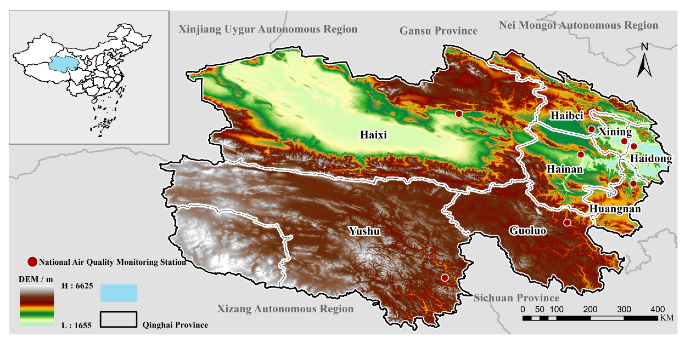
Figure 1. Geographic setting and monitoring network in Qinghai Province.
Sustainability 17 10853 g001
Figure 2. Schematic of the integrated MRG–HSW framework. The framework couples a local-attribution branch (MRG) and an external-transport branch (HSW). In the MRG branch, pollutant–meteorology relationships are quantified using MLR and GAM, and residuals identify potential external influences. The residual-based gate (R) screens high-pollution, high-residual days, which are then analyzed by the HSW branch composed of HYSPLIT trajectory simulations (H), SOM clustering (S), and WCWT source mapping (W). Inputs: daily pollutants (PM2.5, PM10, SO2, NO2, CO; O3 as MDA8), daily meteorology (rh, blh, ssrd, t2m, tp, wind), and 72 h trajectories (00/06/12/18 UTC; heights as specified in the text). Outputs: local-driver metrics (coefficients, t-values, VIF, R2/R2_adj, GAM partial dependence) and external-transport diagnostics (trajectory clusters/frequencies, WCWT potential source regions). Arrows indicate data flow and decision routing.
Sustainability 17 10853 g002
Figure 3. Seasonal and diurnal variations of O3 and PM2.5 at the Xining site during 2020–2024. Lines represent multi-year hourly composites for spring, summer, fall, and winter. (a) O3 concentrations; (b) PM2.5 concentrations.
Sustainability 17 10853 g003
Figure 4. Observed versus predicted O3 and PM2.5 concentrations in Xining from three regression configurations during 2020–2024. (a1) O3 predictions from the pollutant-only regression model; (a2) O3 predictions from the meteorology-only regression model; (a3) O3 predictions from the combined (all-inclusive) regression model; (b1) PM2.5 predictions from the pollutant-only regression model; (b2) PM2.5 predictions from the meteorology-only regression model; (b3) PM2.5 predictions from the combined (all-inclusive) regression model. Insets show the corresponding regression equations, VIF values, and coefficients of determination (R2 and R2_adj).
Sustainability 17 10853 g004
Figure 5. t-values of major variables in the regression models for PM2.5 and O3. (a) The t-values of meteorological factors in the O3 model, and (b) those of pollutant factors in the PM2.5 model. Only the set of factors with the highest explanatory power for each pollutant (as determined by multiple linear regression results) is presented. Asterisks (*) indicate statistical insignificance (p > 0.05).
Sustainability 17 10853 g005
Figure 6. Variation in regression performance (R2) with station elevation for different model configurations. (a) O3 results for the pollutant-only, meteorology-only, and all-inclusive models; (b) PM2.5 results for the pollutant-only, meteorology-only, and all-inclusive models.
Sustainability 17 10853 g006
Figure 7. Comparison of R2 values for O3 (meteorological factors) and PM2.5 (pollutant factors) modeled by MLR and GAM in eight cities of Qinghai Province.
Sustainability 17 10853 g007
Figure 8. Partial dependence of O3 concentration on key meteorological variables with 95% confidence intervals. The x-axis represents the value of each meteorological predictor, while the y-axis shows its marginal effect on the predicted O3 concentration. Shaded areas indicate 95% confidence intervals derived from the standard-error estimates of the GAM smoothing functions. (a) Relative humidity; (b) Boundary layer height; (c) Surface solar radiation downwards; (d) Air temperature (t2m); (e) Precipitation; (f) Wind speed.
Sustainability 17 10853 g008
Figure 9. Partial dependence of PM2.5 concentration on co-pollutant variables with 95% confidence intervals. The x-axis represents the value of each co-pollutant predictor, while the y-axis shows its marginal effect on the predicted PM2.5 concentration. Shaded areas indicate 95% confidence intervals derived from the standard-error estimates of the GAM smoothing functions. (a) O3; (b) PM10; (c) SO2; (d) NO2; (e) CO.
Sustainability 17 10853 g009
Figure 10. Results from the 72 h backward trajectory SOM clustering for O3 high-pollution and high-residual days. (a) Guoluo; (b) Yushu.
Sustainability 17 10853 g010
Figure 11. Results from the 72 h backward trajectory SOM clustering for PM2.5 high-pollution and high-residual days in Guoluo. (a) 500 m; (b) 1000 m; (c) 1500 m.
Sustainability 17 10853 g011
Figure 12. WCWT results of O3 in Guoluo based on SOM-classified trajectories: (a) Cluster A; (b) Cluster B.
Sustainability 17 10853 g012
Figure 13. WCWT results of O3 in Yushu based on SOM-classified trajectories: (a) Cluster A; (b) Cluster B; (c) Cluster C.
Sustainability 17 10853 g013
Figure 14. WCWT results of PM2.5 at 500 m in Guoluo based on SOM-classified trajectories: (a) Cluster A; (b) Cluster B.
Sustainability 17 10853 g014
Figure 15. WCWT results of PM2.5 at 1000 m in Guoluo based on SOM-classified trajectories: (a) Cluster A; (b) Cluster B; (c) Cluster C.
Sustainability 17 10853 g015
Figure 16. WCWT results of PM2.5 at 1500 m in Guoluo based on SOM-classified trajectories: (a) Cluster A; (b) Cluster B; (c) Cluster C.
Sustainability 17 10853 g016
Figure 17. Results from the 72 h backward trajectories for the PM2.5 pollution episode in Guoluo on 28 February 2021. (a) 500 m; (b) 1000 m; (c) 1500 m.
Sustainability 17 10853 g017
Figure 18. Results from the 72 h backward trajectories at 500 m for the O3 pollution episode in Yushu on 1 June 2024.
Sustainability 17 10853 g018
Table 1. Main data sources and variables used in this study.
Data TypeVariable NameResolutionData Source
Air qualityPM2.5, PM10, SO2, NO2, CO, O3Hourly/Daily (O3: MDA8)CNEMC
http://www.cnemc.cn/
Meteorologyrh, blh, ssrd, t2m, tp, windHourly/DailyERA5
https://cds.climate.copernicus.eu/
Meteorological driverGDAS1 fields6-hourlyGDAS1 (NCEP) https://www.ready.noaa.gov/gdas1.php
(accessed on 1 July 2025)
Table 2. City names, site codes, and elevations (m) of air quality monitoring stations included in this study.
CityHaibeiHuangnaHainanGuoluoYushuHaixiXiningHaidong
Site code2671A2672A2673A2674A2675A2676A3055A3129A
Elev. (m)30722471281837183689294222042072
Disclaimer/Publisher’s Note: The statements, opinions and data contained in all publications are solely those of the individual author(s) and contributor(s) and not of MDPI and/or the editor(s). MDPI and/or the editor(s) disclaim responsibility for any injury to people or property resulting from any ideas, methods, instructions or products referred to in the content.