Abstract
We consider a dynamic pricing problem in a double-lane system consisting of one general purpose lane and one wireless charging lane (WCL). The electricity price is dynamically adjusted to affect the lane-choice behaviors of incoming electric vehicles (EVs), thereby regulating the traffic assignment between the two lanes with both traffic operation efficiency and charging service efficiency considered in the control objective. We first establish an agent-based dynamic double-lane traffic system model, whereby each EV acts as an agent with distinct behavioral and operational characteristics. Then, a deep Q-learning algorithm is proposed to derive the optimal pricing decisions. A regression tree (CART) algorithm is also designed for benchmarking. The simulation results reveal that the deep Q-learning algorithm demonstrates superior capability in optimizing dynamic pricing strategies compared to CART by more effectively leveraging system dynamics and future traffic demand information, and both outperform the static pricing strategy. This study serves as a pioneering work to explore dynamic pricing issues for WCLs.
1. Introduction
With increasing environmental awareness, EVs have become mainstream in transportation due to their lower emissions. However, their limited driving range remains a significant obstacle to their full potential. To overcome this challenge, alongside traditional plug-in charging, advanced EV charging methods have been developed, such as static wireless charging, battery swapping, and dynamic wireless charging (DWC). Among these, DWC stands out as the most promising method. It allows EVs to charge while in motion using facilities embedded under the road surface known as wireless charging lanes (WCLs). To date, DWC technology has been researched in many countries, including the United States, China, Germany, Sweden, and Korea. However, most of the research on DWC remains experimental and has not yet been widely implemented in existing traffic systems.
Recognizing the significant potential of DWC, transportation management issues within the DWC context have increasingly attracted academic attention [1]. To date, these issues have been categorized into four aspects: (1) Development and features of DWC technology; (2) Optimal allocation of WCLs [2,3,4,5,6,7,8,9,10,11]; (3) EV energy consumption analysis in WCL context [12,13,14,15,16,17]; and (4) Billing and pricing for EVs on WCLs. Notably, real-time WCL traffic management issues have not been thoroughly studied. Liu et al. [18,19] explored a ramp metering control problem and a variable speed limit (VSL) control problem on WCLs, respectively, which revealed the inherent conflict between traffic operation efficiency and charging service efficiency (defined by the total net energy increase in the EVs). Then, Zhang et al. [20] further included EV routing decisions to ensure smooth traffic on the WCLs, which was shown to partially resolve the trade-off between these two efficiency measures. However, these studies [18,19,20] all assumed that the WCLs are fully deployed on the road system, and therefore their conclusions cannot be extended to more flexible and general lane settings. Some studies, such as [15,16], also highlighted this issue of trade-offs and suggest that WCLs should be deployed in a multi-lane system. However, to our best knowledge, optimizing real-time traffic management in a multi-lane system with WCLs has not been addressed.
In general, the core of real-time management in multi-lane traffic systems focuses on dynamically adjusting traffic assignment across different lanes by adapting to traffic demand. Effective traffic assignment helps optimize lane usage, reduce congestion, and improve overall operational efficiency. In the multi-lane system with WCLs, the goal of real-time management is to optimize both traffic and energy objectives. Therefore, this paper explores a dynamic pricing problem in a double-lane system consisting of one GPL and one WCL. Our basic consideration is that the charging price can influence EVs’ lane choices, thereby affecting the traffic operation and charging service objectives of the system. Therefore, a dynamic pricing strategy is essential to enhance these efficiencies. Given the heterogeneity of EV attributes, the traffic dynamics should be modeled at a micro-level where each EV acts as an autonomous agent. To this end, we employ an Agent-Based Model (ABM) to establish the traffic dynamics. Due to the complexity of the ABM, a model-free method, a deep Q-learning algorithm, is utilized to derive a dynamic pricing strategy.
The primary contributions of this paper are two-fold: (1) we pioneer the exploration of dynamic pricing problems in a multi-lane system with WCLs, thereby filling a significant gap in this field; (2) we propose a novel framework that combines ABM tailored to a multi-lane system with WCLs and deep reinforcement learning (DRL) to derive dynamic pricing strategies. This framework can be applied or extended to other real-time traffic management problems that involve EV choice behavior under the option of DWC.
The remainder of this paper is structured as follows. Section 2 provides a comprehensive review of the related literature, situating our work within the broader context of the field. Section 3 formally defines the problem under investigation, outlining the key considerations and objectives. Section 4 details the research methodology employed, including the theoretical framework and the specific techniques utilized. Section 5 presents the numerical experiments conducted to validate the proposed method, describing the experimental setup, procedures, and evaluation metrics. Section 6 demonstrates and analyzes the results, highlighting the efficacy and implications of our approach. Section 7 summarizes the key findings, draws conclusions, and discusses potential avenues for future research.
2. Related Work
This section presents a brief review of the existing literature related to our study, specifically focusing on three aspects: (1) The pricing problem in traffic systems with WCLs, especially focusing on the scale of the traffic system and the aim of dynamic pricing; (2) Studies on the multi-lane systems with WCLs, especially focusing on the establishment of traffic models and energy consumption models employed within these studies. Additionally, the impact of the integration of WCLs into existing traffic infrastructures on traffic flow dynamics and charging efficiency is of concern; and (3) Studies that apply DRL algorithms in dynamic pricing problems on highways. Our review concentrates on the types of DRL algorithms applied, the route choice models, and the design of state and reward functions.
Several studies have addressed the pricing problems in traffic systems with WCLs. They all consider a static pricing problem on a traffic-network scale. The aim is to reduce costs and promote traffic efficiency. He et al. [21] explored a static pricing problem in WCLs from the perspective of a government agency. The goal is to optimize both transportation and power networks. This study aimed to validate the efficacy of two pricing models, the first and second best, in enhancing social welfare. The first-best model strives to minimize the combined costs of power generation and travel by implementing locational marginal pricing, whereas the second-best model focuses solely on the transportation network, aiming to reduce travel time and energy consumption while ensuring fiscal sustainability. Similarly, Wang et al. [22] also considered a static pricing problem in a network-level traffic system and introduced an intriguing charging pricing and vehicle scheduling algorithm based on a double-level game model. In the lower level, each EV behaves in its self-interest, striving to minimize detours and reduce electricity costs while securing adequate power for travel. The upper level encapsulates the interaction between WCLs and EVs, where EVs seek to lower the charging cost and WCLs aim to maximize profits from electricity sales. This study demonstrates that the proposed double-layer game model can achieve a balanced outcome benefiting both EVs and WCL operators. Similarly to ref. [21], Esfahani et al. [23] also addressed an optimal pricing problem in a DWC scenario, considering both transportation and power networks. However, their focus was on a more advanced scenario where the WCLs are bidirectional, formulating a bi-level optimization problem to determine the optimal buying price for electricity at each charging link, based on the assumption that the selling price is set by the Locational Marginal Price (LMP). The effectiveness of this bidirectional charging model in mitigating peak loads and reducing EV charging costs was substantiated through three numerical examples. It is evident that the extant research concentrates on the network-level pricing problem, presuming the complete coverage of WCLs on a link. And, they all consider a static pricing problem. A dynamic pricing problem multi-lane system with WCLs on a road level has not been addressed.
A few studies address the multi-lane system with deployed WCLs. He et al. [15] developed a car-following model to simulate the driving behaviors of EVs in double-lane systems where the WCL is partially deployed on one lane. This model particularly focuses on the car-following and lane-changing behaviors induced by the presence of WCLs, offering insights into the adjustments that drivers make to utilize charging facilities, which in turn affect overall traffic dynamics and safety. Notably, the authors make some basic assumptions about the traffic rules. For instance, the parameters of all EVs are assumed to be identical. EVs that need charging must choose the WCL, while those that do not require charging may also travel on the WCL. Building on the foundational models and basic assumptions of ref. [15], a subsequent study [16] extended the theoretical framework to quantitatively measure the impacts of WCLs on travel time and energy consumption. This paper not only refines the energy consumption models specific to EVs but also calibrates these models against empirical data, thereby validating the theoretical predictions. The results indicate a notable decrease in road capacity (8% to 17%) and an increase in energy consumption (3% to 14%) under varying traffic densities, underscoring the practical implications of integrating WCLs into existing infrastructures. In contrast, our study focuses on real-time traffic control on WCLs using dynamic pricing, for which a double-lane system is also constructed and simulated. This microscopic way of modeling a dual or multi-lane traffic system is capable of explicitly capturing vehicle-level lane choice decisions, thus enabling refined modeling and the evaluation of control measures, see [24] for a more comprehensive review multi-lane traffic modeling and control. In traditional settings, traffic speed variation is the main factor considered by drivers for lane changing. However, the lane choice and changing decisions of each EV in our problem are mainly driven by its state-of-charge (SOC) due to our focus on WCL management. We develop a DRO-based dynamic pricing controller for managing the two-lane traffic system. Interestingly, the learning-based strategy seems a popular approach in recent studies on traffic control in multi-lane systems, such as for intersection [25] or ramp-merging traffic control [26]. While the control problems in these studies are mostly from the perspective of individual EVs, ours optimizes the traffic operator’s decisions; hence, the underlying system dynamics and uncertainties considered are quite different.
More broadly, the RL-based approaches have been applied to various existing and emerging traffic operational problems with intelligent transportation systems (ITSs), such as traffic signal control [27], variable speed limit control [28], twin-vehicle auto-driving [29], cooperative on-ramp merging control [26] and connected and automated vehicle platooning [30], to name a few recent ones. In particular, several studies have applied DRL algorithms in dynamic pricing problems in highway traffic control, a relevant setting to ours. Pandey et al. [31] explored a dynamic pricing model designed to optimize the use of express lanes. The DRL algorithm utilized here is an Actor–Critic (A2C) algorithm, which is specialized in handling continuous state and action spaces, making it particularly suitable for the dynamic and complex environment of highway traffic. The state representation in this model includes variables such as current traffic density, time of day, and the historical usage patterns of the lanes, while the reward function is designed to maximize revenue and minimize travel time. Abdalrahman and Zhuang [32] extended the application of DRL to manage dynamic pricing in EV charging stations. They employed a multi-agent framework where each charging station operates as an independent agent utilizing a variant of the Q-learning algorithm. The state space for each agent includes the number of EVs waiting, the state of charge of each EV, and the current electricity price, whereas the reward function is constructed to maximize profit while ensuring customer satisfaction by reducing waiting times and charging costs. Cui et al. [33] applied DRL algorithms for dynamic pricing at fast charging stations for EVs, focusing on optimizing station profit and enhancing user satisfaction. The study effectively integrates traffic flow predictions and EV charging demands into a dynamic pricing model that adjusts in real-time to traffic and usage conditions. The study establishes the vehicle–road learning environment using the Markov decision process (MDP) and employs the Deep Deterministic Policy Gradient (DDPG) algorithm, which is a policy-based reinforcement learning method particularly suited for continuous action spaces such as pricing strategies. The state space in the DRL framework includes the current load at the charging stations, the availability of the chargers, the real-time traffic conditions around the stations, and the predicted demand for charging. These variables help the system to understand the current scenario at both the traffic and energy distribution levels. The reward function is designed to maximize the profitability of charging stations while balancing the electrical grid’s demand and user satisfaction.
3. Problem Statement
We consider a dynamic pricing problem in a double-lane system dedicated to providing a charging service for DWC EVs. The system consists of one GPL and one WCL. The speed limit on the WCL is set a bit lower than that on the GPL to extend the charging duration for EVs [15]. In this study, we assume . The entire system is established by NetLogo as an ABM in which an EV is treated as an agent that has attributes including location, current travel speed, SOC, minimum SOC level, etc. The traffic rules in this system are assumed as follows:
- In the lane-changing zone (see Figure 1), each EV can choose one lane. Its lane choice mainly depends on three factors: the current SOC, the observed travel speeds on each lane, and the charging price.
 Figure 1. A schematic diagram of a two-lane road system. The red bar represents the boundary between the two-lane road system and the lane-changing zone.
 - Once an EV enters the GPL or WCL, lane changing behavior is restricted unless its SOC drops below the minimum or exceeds the maximum threshold. All EVs obey this rule, which is enforced by the advanced ITS.
- EVs entering the WCL must charge their battery until their SOC reaches its maximum SOC level.
- The charging price is modeled as a discrete variable and can be changed at regular intervals, e.g., every three minutes.
- EVs receive charging-price information via the ITS with onboard communication support.
- The WCL-equipped traffic system is publicly funded and operated, with the primary goal of maximizing social welfare, that is, minimizing total congestion and maximizing EV energy uptake, rather than profit. Hence, the revenue is not considered.
- Traffic demand and downstream traffic conditions within the control horizon are assumed to be predictable by the system with the support of ITS.
We develop an ABM tailored to the double-lane system in the context of the DWC scenario in NetLogo, as depicted in Figure 1. Since the traffic and charging demands change over time, it is crucial for traffic operators to dynamically adjust the charging prices to influence EVs’ lane choices and optimize traffic distribution between the two lanes. The goal is to enhance the operational efficiency of the system. In this paper, we focus on both traffic operation efficiency and charging service efficiency from the perspective of the system operator. The former efficiency is mainly defined by the traffic throughput as in traditional traffic management settings, while the latter is measured by the total amount of net energy recharged of the EVs, as in the recent literature on WCL traffic control [18,19]. Detailed expressions of these two efficiency measures will be provided in the following section.
Considering the complexity of the ABM, a model-based control method is deemed unsuitable for implementing a dynamic pricing strategy. Instead, a model-free approach based on a deep Q-learning algorithm is derived for the dynamic pricing strategy. Additionally, a straightforward method using the classification and regression tree (CART) algorithm is established as a benchmark approach. We conduct a series of numerical experiments and a case study to demonstrate the effectiveness of the proposed algorithm. The challenges lie in two aspects: (1) the establishment of the ABM tailored to the double-lane system, which involves integrating traffic dynamics and the lane-choice model; and (2) the design of the deep Q-learning algorithm, particularly the formulation of the system state and reward function.
4. Method
This section introduces the basic elements of the ABM and the Deep Q-learning algorithm we adopt. The conceptual design of the interaction between our ABM and the deep Q-learning algorithm is depicted in Figure 2. It can be seen that the ABM (i.e., the environment of the Deep Q-learning algorithm) is coded in NetLogo (introduced in Section 4.2) by extending the existing model “Traffic 2 lanes” in the NetLogo Library [34], which has been used in a number of traffic problems. For example, ref. [35] extends the model to explore the ways to overcome traffic congestion on toll roads. Ref. [36] develops a new traffic simulation environment in NetLogo to explore an intersection control task. In this paper, we incorporate the rules of the double-lane system, depicted in Figure 1, and the SOC dynamics of EVs into the model. Since the deep Q-learning algorithm is coded in Python 3.7, we adopt the pyNetLogo 0.5 library to build the bridge between the algorithm and the environment [37]. The pyNetLogo 0.5 library provides a seamless interface enabling Python to interact with NetLogo. By integrating this library, we are equipped with capabilities to dynamically load models, execute NetLogo-specific commands, and extract data from reporter variables. Such functionalities are instrumental for the training of our deep Q-learning algorithm in an online fashion.
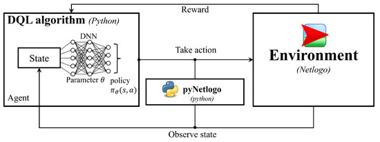
Figure 2.
A schematic diagram of the conceptual design.
4.1. Agent-Based Model (ABM)
The ABM employed for the double-lane road system comprises two types of agents. The first type of agent encompasses the road infrastructure, specifically the GPL and the WCL. The second type of agent is the EV, which is capable of making decisions autonomously and interacting with both the GPL/WCL (i.e., gain energy) and other EVs. The attributes (global variables and EV attributes) of these agents are defined in Table 1.

Table 1.
List of variables.
4.1.1. Global Variables
In our ABM, global variables include speed limits on GPL, speed limits on WCL, charging power, charging price, total throughput, and total energy. Their definitions and notations are as follows.
- Speed limit on GPL (): This denotes the maximum speed at which an EV is permitted to travel on the GPL. In our model, it is defined as a constant. Its unit is km/h.
- Speed limit on WCL (): This denotes the maximum speed at which an EV is permitted to travel on the WCL. Generally, is set slightly lower than to allow EVs more time to charge [15].
- Charging power (e): This denotes the power available at the WCLs, assumed to be constant over time and uniform along the lane, measured in kilowatts (kW).
- Charging price (p): This refers to the cost of charging per kilowatt–hour on the WCL, communicated in real-time to all EVs to facilitate informed lane choices. We assume that p is a discrete variable, priced at USD/kWh.
- Total throughput (): This denotes the cumulative number of vehicles that pass a specific point, such as the entrance of the road, within a given time interval, measured in vehicles per hour (veh/h).
- Total energy (): This denotes the total energy delivered to vehicles via the WCL, calculated as the sum of the energy received by each vehicle, measured in kilowatt–hours (kWh).
Note that only and are statistical accumulators that can change over time, while the other four attributes are assumed to be time invariant.
4.1.2. EV Attributes
Each EV has a set of attributes as follows:
- Maximum travel speed (): This attribute specifies the upper limit of an EV’s speed, normalized to the range . In our model, its value is defined as a constant, which is generally bigger than and .
- Current travel speed (): This attribute describes the instantaneous speed of the EV. Its value is constrained within a normalized range of 0 (stationary) to 1 (maximum travel speed).
- Observed travel speed (,): This attribute captures the speed of EVs within a lane as observed by an individual EV. It is quantified as the average speed of EVs along a specified observable distance (e.g., 100 m) ahead of the observing EV. In this model, we assume it to be the average speed of vehicles across the entire lane, which is disseminated to all vehicles in real time through advanced vehicle communication systems. Its value is normalized to the range .
- Acceleration (): This attribute describes the change of an EV’s speed within one time interval. In our model, their values are defined as constants.
- SOC (): The SOC is a crucial attribute for operations and management on WCLs, indicating the current energy level of the EV’s battery. The value is constrained within a normalized range of 0 (completely depleted) to 1 (fully charged).
- Minimum SOC level (): This threshold represents the critical SOC below which an EV risks imminent power depletion, potentially leading to operational failure and reduced battery lifespan. In our model, an EV is allowed to change to the WCL whenever its SOC level drops below this point.
- Maximum SOC level (): This threshold signifies the optimal SOC at which an EV’s battery is considered fully charged without exceeding the manufacturer’s recommended limits to prevent overcharging. In our model, an EV is allowed to change to the GPL whenever its SOC level exceeds this point.
- Location (): The EV’s location in the context of the NetLogo model is captured by a two-dimensional coordinate , where represents the longitudinal axis along the road while denotes the lateral position across lanes.
- Target location (): This attribute is denoted as the y axis value of the target location of an EV (corresponding to the target lane). In our double-lane system, the GPL and the WCL can be expressed as and , respectively.
- Lateral speed (): This attribute signifies the speed at which an EV executes a lane-changing behavior. In our model, this parameter is defined as a constant.
4.1.3. Exogenous Input
In our model, traffic demand serves as an exogenous input to the double-lane system. Recognizing the possibility that EVs might choose their lanes before reaching the designated lane-changing zone, we assume that EVs appear in their selected lane when they enter the zone if there is available capacity; otherwise, they are compelled to the other lane. This assumption reflects the dynamic interaction between traffic demand and lane availability, ensuring a realistic representation of traffic demand. We also assume that the arrival of EVs into the system within a fixed interval of time (equal to the minimum time interval between two charging price signals, denoted by ) satisfies a Poisson distribution [38]. In this case, the time intervals between consecutive events (an EV enters the system) can be described using an exponential distribution [39]. Then, the inter-arrival times follow an exponential distribution whose probability density function is given by
where the constant rate d represents the vehicles that enter the system per minute, t represents the time interval between consecutive vehicle arrivals. Taking as an example, (1) is plotted in Figure 3.
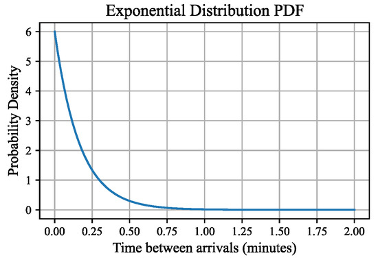
Figure 3.
The time interval between consecutive vehicle arrivals .
In NetLogo, random inter-arrival times are generated from the exponential distribution with the specified rate d. The arrival time for each vehicle is then calculated by the cumulative sum of these random intervals. This process effectively models the stochastic nature of traffic flow into the specified road segment over the given time frame. Note that we simulate a non-homogeneous Poisson process where the rate d changes over time (here, we assume it changes every 3 min) which is approximated by a piecewise constant function. Additionally, we assume that the initial SOC of incoming EVs within a given time frame follows a Gaussian distribution, with a mean () and a standard deviation (). This assumption is consistent with one of the findings yielded in [40] that the SOC distribution of EVs at the beginning of charging events is similar to a Gaussian distribution, with an average initial SOC of around .
4.1.4. Scale
In the NetLogo traffic model, an explicit scale is not defined. Instead, a normalized scale is adopted, wherein the roadway comprises numerous patches, with each vehicle occupying one patch. By assuming that the length of an EV spans four meters, it is inferred that one patch equates to four meters in real-world dimensions. Consequently, this allows for the extrapolation of other parameters, such as speed, on a similar basis. For example, a normalized speed of used in NetLogo corresponds to 80 km/h in reality.
4.1.5. Lane-Choice Model
The probability of lane choices of EVs can be estimated by a discrete choice model, which is a powerful tool used in econometrics and behavioral research to model the decision-making process of individuals faced with multiple alternatives. It was initially proposed by ref. [41] based on random utility theory. The theory assumes that individuals make decisions based on the total utility of available options, which consists of an observable deterministic component related to choice attributes and an unobservable stochastic component that captures individual preferences and random fluctuations. This theory explains why individuals may choose differently under similar conditions and vary their choices over time, highlighting the role of both deterministic influences and stochastic elements in decision making [42]. In this paper, we assume a logit model, which is widely used in predicting drivers’ lane choice among a set of alternatives [43,44,45]. Note that, although our logit model applies to two alternative settings as in our double-lane system, it can be extended to multi-lane systems using a multinomial logit model.
The multinomial logit model for the double-lane system is established in the following. First, we specify two separate utility functions, and , for the two lanes. Each utility function in our model is assumed to be a linear combination of explanatory variables that affect the EVs’ lane choice. In the context of issues related to the pricing of electric vehicle charging, explanatory variables usually include at least SOC, travel time, and charging cost. Since the WCLs have not been commercialized on a large scale, the charging choice in the context of WCLs cannot be well investigated; however, there are studies investigating the charging choice under other scenarios. For instance, ref. [46] analyzed the factors that influence EVs’ charging choice among charging stations using the data from an interactive stated choice experiment. The result shows that the utility of the charging choice is negatively correlated with a set of variables including SOC, charging time, and charging price. Similarly, in our model, we assume that the utility of choosing the GPL for the i-th EV is only influenced by travel time, denoted by , is calculated as the travel time to traverse the selected lane; the utility of choosing the WCL is assumed to be influenced by the charging time, (calculated as the time to charge on the WCL, i.e., the time to traverse the WCL), the SOC (the current SOC of the i-th EV, denoted by ), and charging cost (calculated as the total cost of the EV to charge on the WCL, denoted by ). Then, the utility functions can be expressed as
where the coefficients , , and represent the marginal utilities of SOC, travel time, and charging cost, respectively. are random error terms, which independently and identically follow a Gumbel distribution. is a constant term used to calibrate the utility function. in both utility functions is the SOC of i-th EV at the time it makes the lane-choice; , , and are defined as
where represents the length of the double-lane system. In the equations, we utilize the observed speeds, and , to calculate the expected travel times for the i-th EV traversing the GPL and the WCL, respectively. This calculation is considered reliable in most contexts, provided that the traffic flow speed remains relatively stable over short intervals. The marginal utilities are all negative, indicating that the utility of choosing the lane of an EV decreases with the increase in its SOC, travel/charging time, and charging cost.
Following the traffic rules mentioned in Section 3, we assume that is a piecewise function by dividing the SOC into three ranges, which is similar to the model used in [47]:
where piecewise satisfies the traffic rule that an EV whose SOC is below its minimum SOC level will choose the WCL—while an EV whose SOC exceeds its maximum SOC level will choose the GPL. Then, the choice probability of i-th EV for each lane at time t, denoted as , can be expressed as
The selection of marginal utilities is crucial for the utility functions. In our model, we aim to derive a set of appropriate values for these utilities in Section 5.1 based on the results from [46].
4.1.6. EV Driving Behavior
The behavior of an EV is characterized by the dynamics of its attributes. Among the attributes mentioned in Section 4.1.2, maximum travel speed and acceleration/deceleration are constant, while others are variable. For the i-th EV, its acceleration at time t is calculated as
where and are constants, representing the acceleration magnitudes for EV i when there are no blocking cars ahead and the deceleration magnitude for EV i when there are blocking cars ahead, respectively. Their values can vary slightly across different EVs. is the indicator function that equals 1 if condition c is satisfied and 0 otherwise.
Then, its speed, location along the road, , lateral movement, , can be expressed as
where represents the lateral speed of EVs. In this model, we assume it to be a constant value for all EVs.
As mentioned in Section 4.1.2, the observed travel speeds of EV i on the two lanes, , and are defined as the average speed of vehicles on the entire lane. Let and denote the set of speeds of these observed vehicles on the GPL and WCL, respectively. Then, we have:
where is the total number of vehicles on the lane on which EV i is moving at time t.
Its SOC, , is updated as
where is the charging power of the WCL, which is assumed as a constant. is the energy consumption of i-th EV at time t. Based on the analysis of the laboratory tests from [48], it can be expressed as a nonlinear function of its speed and acceleration :
As discussed in Section 4.1.5, the model for determining the lane choice probability of an EV as it first enters the system is represented by the random variable , with the probability defined as
where represents the probability function which calculates the likelihood of an EV choosing a particular lane for its first entry; here, equals −1 for the choice of the WCL and 1 for the GPL. and are the probabilities for choosing each lane, respectively.
4.2. NetLogo
NetLogo [49] is an agent-based modeling (ABM) platform that enables autonomous agents with distinct behaviors to interact within a shared environment, giving rise to complex system-level phenomena [50]. Recently, NetLogo has been widely adopted in traffic studies, including decentralized routing, distributed coordination, and combined driving–charging behavior [36,51,52,53]). Unlike traditional traffic simulators like VISSIM and SUMO, which are (not agent-based but) more focused on simulating traffic flow based on vehicles, NetLogo emphasizes the behavior and interaction of individual agents. This approach can provide deeper insights into the dynamics of complex systems, such as traffic networks, where individual EV behaviors significantly influence the overall traffic patterns or the heterogeneity among different agents cannot be ignored. Readers interested in more agent-based traffic simulators can refer to [54]. In the traffic scenario explored in this paper, an EV’s lane choice is influenced by multiple attributes, including its location, SOC, charging prices, and observed travel speeds. The heterogeneity of the agents’ attributes is central to the traffic scenario analyzed in this paper and should be taken into account in our approach. Consequently, we employ NetLogo 6.4.0 to simulate the traffic dynamics of a double-lane system.
4.3. Deep Q-Learning Algorithm
Reinforcement learning (RL) is a paradigm of machine learning in which an agent learns to make decisions by performing actions in an environment to achieve a goal. The agent receives feedback in the form of rewards or penalties, guiding it towards effective strategies. The process involves learning what actions to take in different states to maximize the cumulative reward [55]. RL is taxonomized by model usage (model-free vs. model-based) [56], policy representation (policy-based vs. value-based) [57,58], and sampling alignment (on-policy vs. off-policy) [59,60].
Despite RL’s outstanding performance in low-dimensional tasks [55], its scalability to high-dimensional state spaces remains limited. DRL solves this bottleneck by integrating the RL decision-making framework with the expressive function approximation of deep neural networks, allowing the end-to-end learning from raw sensory input while balancing exploration and exploitation [60]. This synergy has produced landmark successes such as AlphaGo [61] and advanced robotic control, yet current DRL algorithms still suffer from sample inefficiency and limited generalization gaps that motivate ongoing research towards more data-efficient and interpretable models.
Given the continuous state representation (traffic density) and discrete action set (charging price), deep Q-learning (DQL), which is one of the most popular value-based RL methods, is adopted in this paper. DQL is a value-based approach that is well suited for problems with a discrete action set and has proven effective across various applications. The choice aligns with our goal to introduce and validate a practical ABM integrated with a DRL framework for real-time pricing in a multi-lane WCL context.
It is important to note that this paper focuses on demonstrating the practicality and effectiveness of this framework rather than engaging in an exhaustive comparison of different RL algorithms. While advanced RL methods such as PPO or A2C could offer additional insights, we emphasize that the choice of RL method should be tailored to the specific demands of the model and the problem it aims to address. Future research could certainly explore these more sophisticated methods to further enhance the dynamic pricing strategies in WCL settings, building upon the foundational work presented here.
4.3.1. Background
Notation
- x—state; a—action; r—reward; —policy; —discount factor.
- —action-value function; —optimal action-value function.
- —network parameters; —loss function with weights .
Traditional Q-learning utilizes a Q-table to estimate the maximum expected rewards for an optimal action a for a given state x in a specific environment [62,63]. Let be the optimal action-value function which denotes the maximum expected return achievable by any policy, given state x and action a. By the Bellman optimality equation, is defined as
However, tabular Q-learning fails in large or continuous state spaces [64]. DQL replaces the Q-table with a neural network that maps states to Q-values, enabling generalization across high-dimensional inputs. Training minimizes the squared TD-error:
where the expectation is over transitions sampled from the behavior policy induced by Q. This gradient-based optimization yields an effective approximation of in complex domains.
4.3.2. State
The state consists of traffic states and the future traffic demand. For the representation of traffic states, we first divide the road system under consideration into N segments (each segment is assumed to be identical), as depicted in Figure 4. Let be the vectors collected the normalized traffic densities on the GPL and the WCL, respectively, (The state space is deliberately macroscopic: it encodes only the number of EVs per segment. This is sufficient because the pricing policy acts on aggregate lane-choice probabilities rather than on individual trajectories. Microscopic uncertainties average out at the segment level, and any residual error can be reduced by shortening the segment length. When RL is employed for micro-control tasks that involve vehicle-level actions, on the other hand, the state representation should explicitly account for the positions and speeds of individual EVs [26,29].). Then, we have
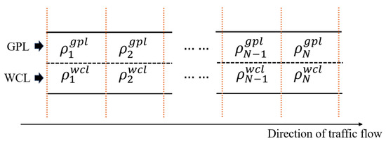
Figure 4.
Road segments.
Here, the n-th normalized traffic density, and , are defined as
where and are the numbers of EVs located within the n-th segments on the GPL and the WCL; and represents the maximum number of vehicles that can be accommodated within the segment.
Similarly, we use a vector to represent the future traffic demand over the next periods of pricing signals. Here, for is the average number of incoming vehicles per minute within the i-th period in the future, which is equal to the d adopted in Section 4.1.3. is the pre-defined maximum value of . Let the system state can be expressed as
Note that all elements in the state have been normalized to fall within the range .
4.3.3. Action
The action within our DRL framework is the charging price, denoted by (its unit is USD/kWh). The base price is set to be . In our model, we adopt a fixed marginal utility for each price; however, in some cases, a piece-wise marginal utility can be assumed, as demonstrated in ref. [65].
4.3.4. Reward
The reward is derived from two objectives: maximizing the traffic operation efficiency measured by total throughput [66] and the charging service efficiency measured by the total net energy delivered to EVs [18,19] (i.e., the total energy received minus consumed), while penalizing any deviation from critical densities to discourage congestion.
The reward at time t is given by
where is the number of vehicles passing the loop detector at the WCL entrance during interval t (see Figure 4); is the total net energy recharged to EVs; and are congestion penalties over all N segments, modeled by the sigmoid variant proposed in [67]:
which yields near-zero penalty when the density of a segment is below its critical density, and rapidly increases thereafter, mirroring the soft-constraint approach adopted in DRL algorithms. The weights allow the flexible balancing of these objectives [68]. , , , are the coefficients of the penalty function. These parameters determine the scaling and translation of the function which can be user-defined.
4.3.5. Q-Network
In the proposed algorithm, the state vector has been defined in (25), then the Q-network approximates the Q-value function , which comprises a series of fully connected (FC) layers interspersed with nonlinear activation functions. Here, we adopt the Rectified Linear Unit (ReLU) as the activation function.
4.3.6. Training
Episodic reinforcement learning: In an episodic reinforcement learning, each training run is decomposed into episodes that terminate after a fixed number of steps. The initial state is sampled from a distribution over traffic densities, ensuring that the agent experiences diverse congestion patterns. Within every episode, the agent executes actions, collects transitions, and periodically updates the Q-network via experience replay, thereby maximizing the discounted return over the trajectory while mitigating long-horizon credit assignment and sparse-reward issues. Full details are given in Algorithm 1.
Exploration rate: DRL typically uses a decaying exploration rate (e.g., epsilon-greedy with decaying ) to shift the agent from broad exploration early on to the later exploitation of learned knowledge, avoiding premature convergence while maximizing long-term reward. In the proposed algorithm, the decay of is modeled by the following formula, where , , and represent the initial exploration rate, final exploration rate, and the decay factor, respectively:
Here, t represents the frame index or the number of iterations. This formula ensures that decreases exponentially from to , reducing as the agent gains more experience, thereby transitioning from exploration to exploitation.
Experience replay: To mitigate the non-stationarity and sample correlation inherent in sequential RL updates, we equip the agent with an experience replay buffer that stores every transition . During the training process, the algorithm randomly samples a minibatch of experiences from the replay buffer.
| Algorithm 1 Deep Q-learning with experience replay |
| Require: : discount factor, : learning rate, : exploration rate |
| Require: C: memory capacity for experience replay, M: minibatch size |
|
4.4. The CART Algorithm
Decision trees are a fundamental type of machine learning algorithm used for both classification and regression tasks, modeling decisions and their consequences in a tree structure [69]. The nodes represent features tests, while the branches correspond to the outcomes of these tests. Among the foundational algorithms, ID3 uses information gain to select the best feature for splitting data [70], whereas CART employs Gini impurity for classification and mean squared error (MSE) for regression [71]. These methods have been extended, such as C4.5, which handles both continuous and discrete attributes and employs sophisticated pruning techniques [72].
For regression, CART keeps splitting until the MSE of every subset is as small as possible. The MSE is defined as
where is the actual value, is the predicted value, and n is the number of data points in the subset.
In this paper, the CART algorithm is employed to generate a preliminary dynamic pricing strategy by leveraging one-step performance data derived from sample scenarios (see Section 5). The CART algorithm is selected because of its inherent suitability for the data structure of the dynamic pricing problem, which aligns with the characteristics of the data set and the nature of the problem. In the following, the training procedure is introduced.
Training
In this study, we develop a dynamic pricing strategy using the CART algorithm, primarily to establish a benchmark for evaluating our DQL algorithm, rather than to fully explore the potential of traditional machine learning techniques. Considering that the price p is a discrete variable, the dynamic pricing challenge could initially be approached as a classification task. However, such an approach fails to leverage the continuous value data of each price p, which is crucial for a nuanced understanding of pricing dynamics. To address this limitation, we employ the CART algorithm for a regression task to better utilize the quantitative information associated with each potential price. Our methodology unfolds in three steps:
- 1.
- Data generation: Utilizing an Agent-Based Model (ABM), we generate a dataset , where comprises the feature vector. Here, represents the state, specifically only including the immediate future traffic demand, distinct from the states used in DQL. The action a is also included in X. The corresponding consists of the rewards for each charging price p, illustrating the reward’s dependency on the price.
- 2.
- Decision tree training: We apply the CART algorithm to map the relationship between X and Y (as defined in (26)), thereby modeling how different charging prices influence the rewards. The purity of each node is measured using the MSE.
- 3.
- Optimal price implementation: The price yielding the highest reward is selected and implemented in the system, optimizing the charging strategy within the defined parameters.
Our aim is to test the efficacy of the DQL algorithm by comparing it against a straightforward, regression-based benchmark. The pseudocode of the algorithm is detailed in Algorithm 2.
| Algorithm 2 Modified CART |
|
5. Numerical Experiments
5.1. Parameter Settings for the Lane-Choice Model
As detailed in Section 4.1.5, the marginal utilities in our logit model are informed by the results from ref. [46], where the corresponding values are , , and for the variables , , and , respectively. These variables represent SOC in percentage, charging time in hours, and charging cost in dollars. It is crucial to note that in the cited study, and denote the time and cost to fully charge an EV’s battery. However, in the WCL context, it is not feasible for an EV to achieve a predetermined SOC since the charging duration is equivalent to the time taken to travel the entire WCL. Given this discrepancy in the definition of and , we adapt the marginal utilities in our model by considering the relative values of different variables, rather than directly adopting the values from the cited reference. In our model, we assume that all EVs share the same battery capacity of 75 kWh; the actual power of WCL, , is 15 kW. Other parameters are collected in Table 2.
Table 2.
Values of the double-lane system.
First, since and are calculated in the same way, it can be inferred that
According to the coefficients of SOC and charging cost, the value of a 1% decrease in SOC is calculated as (), indicating that a 1% reduction in SOC equates to a decrease of USD 4.58 in the total charging cost when charging from the current SOC to full capacity. For example, if we assume that the current SOC of EVs is 41% [40], then the equivalent charging cost per kWh that corresponds to the same financial impact as a 1% SOC decrease is calculated as USD/kWh. Then, we have . Hence, the ratio of to can be calculated as
Let . Based on Equations (30) and (31), we calculate that and . To emphasize the impact of charging price on lane choice, we increase the coefficient for by 1.5 times, resulting in . The relationship between the probability of choosing the WCL and the charging price , for an EV with a SOC of 41%, is illustrated in Figure 5.
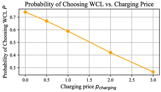
Figure 5.
The relationship between the probability of choosing the WCL and the charging price, assuming an EV with an SOC of 41%.
However, it is important to note that these marginal utilities are only for reference. Accurate values should be derived from experimental analysis in the context of WCLs. Nonetheless, this is difficult to implement before the large-scale commercialization of WCLs.
5.2. Simulation for Sample Scenarios
In this section, we conduct a series of numerical experiments across twelve sample scenarios. In each scenario, we test the performance of every possible charging price. Hence, each scenario only lasts for one pricing interval. The objectives of these experiments are three-fold: (1) to demonstrate the effectiveness of our ABM developed in NetLogo, (2) to validate the design of the reward function as defined in Equation (26), and (3) to elucidate the performance disparities among various charging prices .
The initial conditions of the twelve scenarios are detailed in Table 3, where and represent the total number of EVs on the GPL and on the WCL, respectively. In scenarios #1 to #4, the system begins with free-flow traffic, whereas scenarios #5 to #8 and #9 to #12 start with medium and heavy congestion, respectively. To facilitate the consistent comparison of different charging prices (), a uniform highway traffic demand of is maintained across all scenarios. This setup is designed to encompass a broad range of traffic conditions, providing a comprehensive analysis of the impacts of pricing strategies. The performance of each price setting () within a scenario is determined by averaging the outcomes of ten repeated experiments, enhancing the reliability of our results.
Table 3.
Initial states for the numerical examples.
5.3. Parameter Settings for the Deep Q-Learning Algorithm
This section introduces the parameter settings for the DQL algorithm. First, the parameters for the ABM used in the numerical experiments and the hyperparameters for the DQL algorithm are listed in Table 2. During the process of DQL training, in each episode, the system begins with a random initial state wherein the total number on the GPL and the WCL satisfy a uniform distribution: , . The variation in the initial state across different episodes helps enhance the algorithm’s ability to address diverse traffic dynamics. Each episode lasts for 10 pricing intervals of 30 min. Hence, T in Step 5 of Algorithm 1 is set to be 10.
5.4. Parameter Settings for the CART Algorithm
In this section, we introduce the configuration of the training data and the hyper-parameter settings employed for the CART algorithm. The training dataset, constructed from the twelve illustrative scenarios discussed in Section 5.2 and outlined in Table 3, comprises 60 data points resulting from a combination of 12 scenarios and 5 distinct pricing levels. For each data point, traffic demands are selected from a set , generating 300 unique combinations. We believe that these 300 data points can cover most traffic scenarios. We set the maximum depth to 4, require at least 10 samples for any split, and allow no fewer than 5 samples in each leaf. These values keep the tree shallow and the splits data-rich enough to curb over-fitting while still capturing the main pricing patterns; with limited depth, the model avoids high-variance leaf rules, and the sample thresholds ensure that each rule is backed by enough observations to generalize well to new traffic states. The model is evaluated using the testing subset. Predictions for the test features are generated and then compared against the actual outcomes in the test dataset. The MSE is used to evaluate the average squared difference between the predicted values and the actual values. A lower MSE value indicates higher model accuracy and better performance in capturing the underlying data patterns.
5.5. Simulation of Real Traffic Scenarios
In this subsection, we construct two real traffic scenarios that facilitate a comparative analysis between the DQL algorithm and the CART algorithm. Each scenario spans 30 min, corresponding to 10 pricing intervals. In Scenario #1, the system initiates under conditions of light traffic, replicating a typical morning traffic scenario with low demand persisting for 30 min. Conversely, Scenario #2 starts with heavy traffic, characterized by greater congestion on the WCL compared to the GPL, and maintains high traffic demand throughout the same duration.
We employ real-world traffic data used in [18], , as illustrated in Figure 6, to model the demand within our double-lane system. The traffic demand data is sampled every 3 min, aligning with the pricing interval. In the NetLogo environment, the arrival pattern of incoming EVs is modeled according to a Poisson distribution, as delineated in Section 4.1.3.
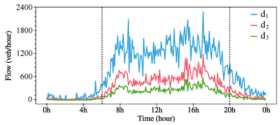
Figure 6.
Real traffic demand for numerical experiments.
In each scenario, both the DQL and CART algorithms generate 10 pricing signals. To underscore the impact of charging prices on traffic flow and charging efficiencies, we also evaluate the performance of a constant pricing strategy (here, we adopt the base price, 1 USD/kWh). The efficacy of the three strategies is compared in terms of total throughput, total energy received by EVs, and the penalties for congestion, consistent with the reward function defined in (26).
6. Results and Discussions
6.1. Results for Sample Scenarios
Figure 7 displays the results of the first four numerical experiments conducted under an initial state of free-flow traffic. Among these experiments, it is observed that the lowest charging price results in the best reward. The reasons are intuitive. Firstly, it can be noted that the total throughput across different charging prices is almost the same in all four experiments. This is because the light initial traffic conditions allow incoming EVs to enter the double-lane system without experiencing congestion, regardless of how traffic demand is allocated between the two lanes. It can also be observed that the penalty for traffic congestion in each experiment remains at a low level (<0.04) in the four scenarios. Hence, the total energy dominates the reward according to (26). The lowest charging price () results in more EVs choosing the WCL compared to other prices, thereby yielding the highest total energy.
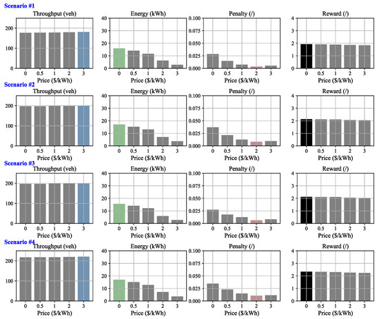
Figure 7.
Results for sample scenarios 1 to 4, characterized by an initial state of free-flow traffic. Note that, in each figure, the colored bars (blue, green, red, black) represent either the maximum or the minimum values, while the other bars are shown in grey.
Figure 8 and Figure 9 display the results of the first four numerical experiments conducted under initial states of medium and heavy traffic, respectively. In scenarios #7, #8, and #11, where the GPL is more congested than the WCL, a lower price results in more EVs choosing the WCL, which not only eases the congestion on the GPL (indicated by a lower penalty), but also increases the total throughput and improves the total energy received by EVs. Consequently, the lowest price exhibits the best reward. In contrast, in scenarios #5, #6, and #10, where the WCL is more congested than the GPL, a higher price leads to more EVs choosing the GPL, effectively easing the congestion on the GPL (lower penalty) and increasing total throughput. Although a lower price still exhibits a higher total energy received by EVs, in the context of congested traffic, the penalty and the total throughput dominate. Consequently, the best rewards are achieved at prices of in these scenarios, respectively. In scenarios #9 and #12, where the congestion on both lanes is about the same, a medium price (1 USD/kWh) performs best considering the trade-off between the three metrics.
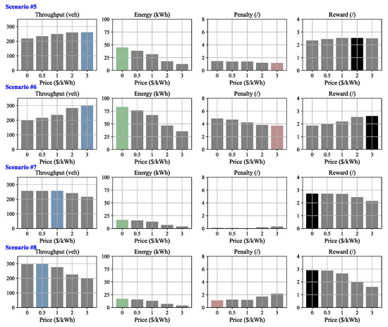
Figure 8.
Results for sample scenarios 5 to 8, characterized by an initial state of congested (medium) traffic. Note that, in each figure, the colored bars (blue, green, red, black) represent either the maximum or the minimum values, while the other bars are shown in grey.
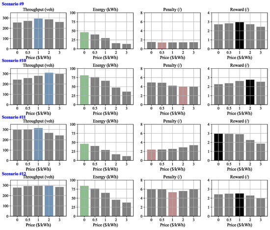
Figure 9.
Results for sample scenarios 9 to 12, characterized by an initial state of congested (medium) traffic. Note that, in each figure, the colored bars (blue, green, red, black) represent either the maximum or the minimum values, while the other bars are shown in grey.
The results provide useful managerial insights for operating WCLs. Traffic operators can effectively optimize traffic flow by dynamically adjusting the charging price. When the WCL is more congested, raising the price shifts EVs to the GPL, easing congestion at the cost of WCL utilization; interestingly, when the GPL is more congested, lowering the price attracts EVs to the WCL, reducing congestion while simultaneously improving WCL utilization—a win–win outcome.
6.2. Learning Performance of the Decision Tree Algorithm
The performance of the Decision Tree Regression model was evaluated using both the mean squared error (MSE) and the coefficient of determination (). These metrics collectively provide a comprehensive view of the model’s predictive accuracy and its ability to explain the variability in the target variable.
The MSE provides a measure of the average of the squares of the errors, indicating how closely the model’s predictions match the actual values:
In addition, is calculated to assess the proportion of variance in the dependent variable that is predictable from the independent variables:
where is the mean of the observed data .
The model achieved an MSE of 0.054, indicating a strong predictive accuracy with minor deviations from the actual values. Additionally, the value obtained was 0.85, suggesting that 85% of the variance in the dependent variable is explainable by the independent variables. This high value corroborates the model’s effectiveness in capturing and quantifying the underlying data patterns. The combination of a low MSE and a high demonstrates not only the model’s ability to produce accurate predictions but also its capacity to explain a significant proportion of the variance in the data.
6.3. Learning Performance of Deep Q-Learning
In this section, we demonstrate the learning performance of our DQL algorithm, as depicted in Algorithm 1. Figure 10 illustrates the learning curves for Algorithm 1. We conduct five repeated trainings under the same parameter settings. It is observed that the cumulative reward per episode progressively increases over time, albeit with some fluctuations. In the initial 50 episodes, where the exploration rate is high, the rewards garnered are modest, reflecting the agent’s preliminary adaptation and exploration of the environment. As training advances, a notable increase in rewards is seen between episodes 50 and 150, denoting the agent’s improved performance and strategy optimization. Beyond 200 episodes, the rewards reach and maintain a relatively high plateau, highlighting the agent’s successful derivation of an effective policy through sustained training.
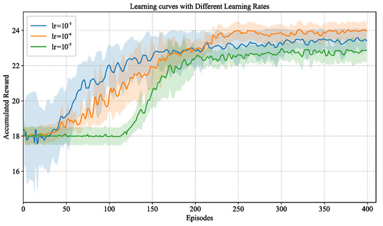
Figure 10.
Accumulated reward vs. episodes for Algorithm 1. The solid line represents the average performance over ten repeated trainings. The shaded region represents half of the standard deviation from the average performance.
Furthermore, Figure 10 compares the impacts of different learning rates on the convergence behavior. When the learning rate is high (1 × ), the algorithm converges more rapidly in the early stages but exhibits larger variance, suggesting instability in value estimation and a tendency to overshoot the optimal policy. With a moderate learning rate (1 × ), the learning curve demonstrates both stable growth and efficient convergence, ultimately achieving higher asymptotic performance. Conversely, a very small learning rate (1 × ) results in much slower convergence, as the agent requires more episodes to sufficiently update its value function. Therefore, we adopt the learning rate of 1 × in the following numerical experiments.
6.4. Results Under Real Traffic Scenarios
This section compares the performance of three strategies within the two real traffic scenarios. Figure 11 and Figure 12 plot the price signal under the two scenarios. Figure 13 and Figure 14 compare the efficacy of these strategies across four critical metrics: accumulated reward, total throughput, total energy, and penalties for congestion, corresponding to scenario #1 and scenario #2, respectively.
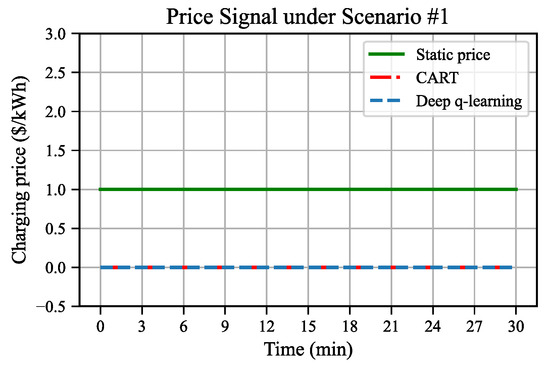
Figure 11.
Price signal for real traffic scenario #1.
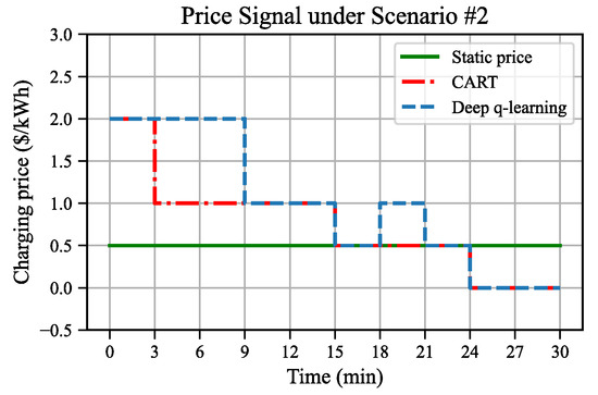
Figure 12.
Price signal for real traffic scenario #2.
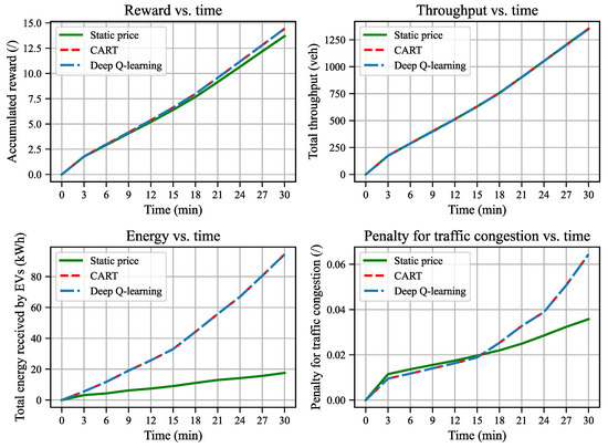
Figure 13.
Results for the real traffic scenario #1.
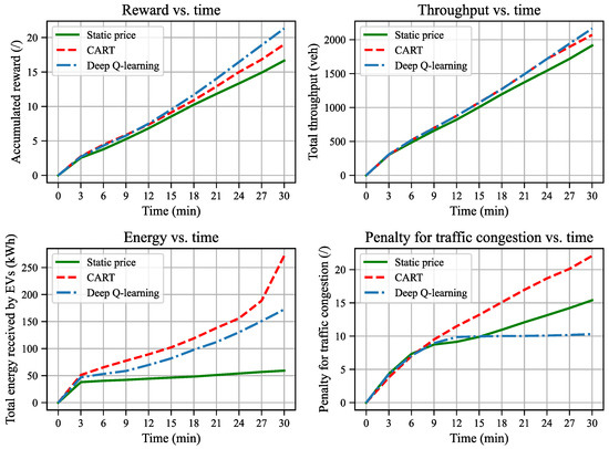
Figure 14.
Results for real traffic scenario #2.
In scenario #1, where the system begins with light traffic and experiences a low traffic demand, both the CART and DQL algorithms consistently opt for the lowest charging price (0 USD/kWh) at each pricing interval throughout the simulation. This leads to an increase in the number of EVs entering the WCL, thereby resulting in more energy being transmitted to EVs. This phenomenon aligns with the analysis in Section 6.1, indicating that a lower charging price under light traffic conditions enhances the charging efficiency without sacrificing the traffic efficiency. The strategy of giving the base price (1 USD/kWh) throughout the simulation yields a total throughput of 1349 veh, a total energy of 17.6 kWh, and a penalty of 0.036. In contrast, the CART and DQL algorithms yield almost the same total throughput, over five times energy (94.4 kWh), but a bit higher penalty for traffic congestion (0.064, however, still at a low level). Consequently, the accumulated reward yielded by the dynamic pricing strategy is 6.7% higher than the static pricing strategy.
In scenario #2, the system starts under heavy traffic conditions with sustained high demand throughout the simulation. As illustrated in Figure 14, the pricing trends demonstrated by the CART and DQL algorithms start at a high price (2 USD/kWh) and progressively decrease, culminating in the minimum price (0 USD/kWh). The DQL algorithm shows performance improvements in the final reward of 12.1% over CART and 28.3% over the static pricing strategy. The reasons are as follows. As the initial congestion on the WCL is greater than that on the GPL, both algorithms implement a high price (2 USD/kWh) at the beginning. This effectively leads more EVs to the GPL, alleviating congestion on the WCL. Subsequently, as congestion eases, the focus shifts towards maximizing energy transmission, leading to lower prices. In the final stages (24 to 30 min), the system reverts to light traffic conditions, similarly to scenario #1, where a lower price is advantageous for maximizing energy delivery without compromising traffic efficiency. However, the pricing strategies of CART and DQL differ significantly. CART is not capable of capturing the system dynamics or utilizing the future traffic demand information but only selects optimal prices for the current interval. Although the traffic demand remains high throughout the simulation, CART still adopts a more aggressive pricing approach at the early stages to maximize the immediate rewards. In contrast, the DQL algorithm adopts a more nuanced strategy, maintaining a lower price of 1 USD/kWh between 3 and 9 min, which, despite temporarily reduces energy growth, minimizes congestion penalties and enhances throughput. Consequently, from 9 to 15 min, the energy growth under both strategies aligns, yet the congestion penalty remains significantly lower under the DQL approach. Thus, CART’s strategy is myopic, whereas DQL’s farsighted approach better captures the complexities of the environment and effectively leverages the future system inputs, highlighting its superior capability in managing complex dynamic traffic scenarios.
In summary, in light traffic scenarios, the dynamic pricing strategy tends to give as low a price as possible. It greatly improves the charging service efficiency and only slightly compromises on traffic operation efficiency. Since the traffic dynamics under light traffic is simple, CART and DQL exhibit a similar performance. However, in heavy traffic, the DQL algorithm outperforms the CART due to its ability to capture the complex system dynamics of the ABM and leverage future traffic demand information. Under both light and traffic scenarios, the two dynamic pricing strategies, which can give a charging price in correspondence to the system state, performs better than the static pricing strategy.
6.5. Model Validation and Calibration
The proposed NetLogo-based traffic model is mainly based on synthetic parameters and traffic data, which may affect the model accuracy. At present, the only commercial DWC system is the bus-transit route in Korea [2]; passenger-car EV data for WCLs are therefore unavailable. Once DWC adoption expands, three aspects of the model will need validation and calibration: (1) the microscopic driving behavior parameters listed in Table 1; (2) lane-choice model parameters; and (3) the EV energy consumption profile, since real-world use on a WCL may differ from the baseline profile taken from conventional roads. Furthermore, the long-term demand profile using the WCL system with dynamic pricing and automatic billing may be affected by user adoption behavior as observed for other advanced transportation technologies [75]; thus, model calibration may be updated every few years to reflect changes in travel behavior patterns.
7. Conclusions and Future Work
This study examines a dynamic pricing problem in a double-lane traffic system consisting of a GPL and a WCL. The system is modeled using an agent-based framework, where each EV is represented as an autonomous agent. A DQL algorithm is developed to determine the optimal pricing strategy, dynamically adjusting charging prices to balance traffic and charging efficiencies. Numerical experiments demonstrate that the DRL strategy substantially outperforms both a CART-based strategy and a static pricing approach, owing to its ability to exploit system dynamics and anticipate future demand. The results underscore the potential of the value-based RL framework for the discrete pricing of WCLs, which is much more effective than the myopic and static policies. Our findings also provide useful managerial insights: when the GPL is congested and the WCL is underutilized, reducing the WCL price can simultaneously enhance traffic and charging efficiencies, creating a win–win outcome. Conversely, when the WCL is congested, dynamic pricing must carefully balance the trade-off between the two efficiencies.
Future research can extend this work in several directions. First, the ABM can be enriched with more realistic and heterogeneous EV characteristics, such as diverse battery capacities, charging rates, and driving behaviors. Second, the DRL framework can be enhanced through improved hyperparameter tuning, more expressive state representations, and refined reward functions to accelerate convergence and improve stability. Though we have discussed the impact of learning rate, global sensitivity analysis that is seen in other transportation studies (e.g., [76,77]) can be performed to more thoroughly pinpoint the most critical parameters of the proposed learning algorithm. Third, broader algorithmic benchmarking can also be explored to enrich the choices of DRL methods for the problem, as we mentioned earlier. Fourth, new elements of the optimization model can be explored. For example, specific constraints can be introduced to avoid notable disproportional service for EVs with lower charging needs [19], thus improving the fairness of the dynamic pricing model—whilst revenue objectives that are not considered in this paper represent a natural avenue for further study. Finally, the current framework assumes the availability of mature vehicle communication systems and a high penetration of EVs using DWC [78]. Before such conditions are achieved, alternative traffic management strategies should be explored to address the mixed traffic flows of DWC-enabled and conventional vehicles, ensuring smooth integration during the transition phase.
Author Contributions
Conceptualization, F.L. and Z.T.; methodology, F.L. and Z.T.; software, F.L.; validation, F.L. and Z.T.; formal analysis, F.L. and Z.T.; investigation, F.L.; resources, Z.T. and H.K.C.; writing—original draft preparation, F.L.; writing—review and editing, Z.T. and H.K.C.; visualization, F.L.; supervision, Z.T. and H.K.C.; project administration, Z.T.; funding acquisition, F.L. All authors have read and agreed to the published version of the manuscript.
Funding
This paper is partially supported by Science and Technology Planning Project of Shandong Hi-speed Group Co., Ltd. (No. HS2025B018).
Institutional Review Board Statement
Not applicable.
Informed Consent Statement
Not applicable.
Data Availability Statement
The original contributions presented in this study are included in the article. Further inquiries can be directed to the corresponding author.
Conflicts of Interest
Author Fan Liu is an employee of Shandong Hi-speed Group Co., Ltd. This research was partly funded by Shandong Hi-speed Group Co., Ltd. All authors have disclosed no other commercial or financial relationships that could be construed as a potential conflict of interest beyond the employment and funding relationships noted above.
References
- Tan, Z.; Liu, F.; Chan, H.K.; Gao, H.O. Transportation systems management considering dynamic wireless charging electric vehicles: Review and prospects. Transp. Res. Part E Logist. Transp. Rev. 2022, 163, 102761. [Google Scholar] [CrossRef]
- Miller, J.M.; Jones, P.T.; Li, J.M.; Onar, O.C. ORNL experience and challenges facing dynamic wireless power charging of EV’s. IEEE Circuits Syst. Mag. 2015, 15, 40–53. [Google Scholar] [CrossRef]
- Lee, M.S.; Jang, Y.J. Charging infrastructure allocation for wireless charging transportation system. In Proceedings of the Eleventh International Conference on Management Science and Engineering Management 11, Changchun, China, 17–19 August 2018; Springer: Berlin/Heidelberg, Germany, 2018; pp. 1630–1644. [Google Scholar]
- Chen, Z.; He, F.; Yin, Y. Optimal deployment of charging lanes for electric vehicles in transportation networks. Transp. Res. Part B Methodol. 2016, 91, 344–365. [Google Scholar] [CrossRef]
- Chen, Z.; Liu, W.; Yin, Y. Deployment of stationary and dynamic charging infrastructure for electric vehicles along traffic corridors. Transp. Res. Part C Emerg. Technol. 2017, 77, 462–477. [Google Scholar] [CrossRef]
- Alwesabi, Y.; Wang, Y.; Avalos, R.; Liu, Z. Electric bus scheduling under single depot dynamic wireless charging infrastructure planning. Energy 2020, 213, 118855. [Google Scholar] [CrossRef]
- Ngo, H.; Kumar, A.; Mishra, S. Optimal positioning of dynamic wireless charging infrastructure in a road network for battery electric vehicles. Transp. Res. Part D Transp. Environ. 2020, 85, 102393. [Google Scholar] [CrossRef]
- Mubarak, M.; Üster, H.; Abdelghany, K. Strategic network design and analysis for in-motion wireless charging of electric vehicles. Transp. Res. Part E Logist. Transp. Rev. 2021, 145, 102159. [Google Scholar] [CrossRef]
- Liu, H.; Zou, Y.; Chen, Y.; Long, J. Optimal locations and electricity prices for dynamic wireless charging links of electric vehicles for sustainable transportation. Transp. Res. Part E Logist. Transp. Rev. 2021, 145, 102174. [Google Scholar] [CrossRef]
- Alwesabi, Y.; Liu, Z.; Kwon, S.; Wang, Y. A novel integration of scheduling and dynamic wireless charging planning models of battery electric buses. Energy 2021, 230, 120806. [Google Scholar] [CrossRef]
- Schwerdfeger, S.; Bock, S.; Boysen, N.; Briskorn, D. Optimizing the electrification of roads with charge-while-drive technology. Eur. J. Oper. Res. 2022, 299, 1111–1127. [Google Scholar] [CrossRef]
- Deflorio, F.P.; Castello, L.; Pinna, I.; Guglielmi, P. “Charge while driving” for electric vehicles: Road traffic modeling and energy assessment. J. Mod. Power Syst. Clean Energy 2015, 3, 277–288. [Google Scholar] [CrossRef]
- Deflorio, F.; Pinna, I.; Castello, L. Dynamic charging systems for electric vehicles: Simulation for the daily energy estimation on motorways. IET Intell. Transp. Syst. 2016, 10, 557–563. [Google Scholar] [CrossRef]
- García-Vázquez, C.A.; Llorens-Iborra, F.; Fernández-Ramírez, L.M.; Sánchez-Sainz, H.; Jurado, F. Comparative study of dynamic wireless charging of electric vehicles in motorway, highway and urban stretches. Energy 2017, 137, 42–57. [Google Scholar] [CrossRef]
- He, J.; Huang, H.J.; Yang, H.; Tang, T.Q. An electric vehicle driving behavior model in the traffic system with a wireless charging lane. Phys. A Stat. Mech. Its Appl. 2017, 481, 119–126. [Google Scholar] [CrossRef]
- He, J.; Yang, H.; Huang, H.J.; Tang, T.Q. Impacts of wireless charging lanes on travel time and energy consumption in a two-lane road system. Phys. A Stat. Mech. Appl. 2018, 500, 1–10. [Google Scholar] [CrossRef]
- Jansuwan, S.; Liu, Z.; Song, Z.; Chen, A. An evaluation framework of automated electric transportation system. Transp. Res. Part E Logist. Transp. Rev. 2021, 148, 102265. [Google Scholar] [CrossRef]
- Liu, F.; Tan, Z.; Chan, H.K.; Zheng, L. Ramp Metering Control on Wireless Charging Lanes Considering Optimal Traffic and Charging Efficiencies. IEEE Trans. Intell. Transp. Syst. 2024, 25, 11590–11601. [Google Scholar] [CrossRef]
- Liu, F.; Tan, Z.; Chan, H.K.; Zheng, L. Model-based variable speed limit control on wireless charging lanes: Formulation and algorithm. Transp. Res. Part E Logist. Transp. Rev. 2025. [Google Scholar] [CrossRef]
- Zhang, Y.; Hong, Y.; Tan, Z. Design of Coordinated EV Traffic Control Strategies for Expressway System with Wireless Charging Lanes. World Electr. Veh. J. 2025, 16, 496. [Google Scholar] [CrossRef]
- He, F.; Yin, Y.; Zhou, J. Integrated pricing of roads and electricity enabled by wireless power transfer. Transp. Res. Part C Emerg. Technol. 2013, 34, 1–15. [Google Scholar] [CrossRef]
- Wang, T.; Yang, B.; Chen, C. Double-layer game based wireless charging scheduling for electric vehicles. In Proceedings of the 2020 IEEE 91st Vehicular Technology Conference (VTC2020-Spring), Antwerp, Belgium, 25–28 May 2020; pp. 1–5. [Google Scholar]
- Esfahani, H.N.; Liu, Z.; Song, Z. Optimal pricing for bidirectional wireless charging lanes in coupled transportation and power networks. Transp. Res. Part C Emerg. Technol. 2022, 135, 103419. [Google Scholar] [CrossRef]
- Lei, X.; Li, L.; Li, G.; Wang, G. Review of multilane traffic flow theory and application. J. Chang. Univ. (Nat. Sci. Ed.) 2020, 40, 78–90. [Google Scholar]
- Jiang, J.; Ren, Y.; Guan, Y.; Eben Li, S.; Yin, Y.; Yu, D.; Jin, X. Integrated decision and control at multi-lane intersections with mixed traffic flow. J. Phys. Conf. Ser. 2022, 2234, 012015. [Google Scholar] [CrossRef]
- Zhou, S.; Zhuang, W.; Yin, G.; Liu, H.; Qiu, C. Cooperative on-ramp merging control of connected and automated vehicles: Distributed multi-agent deep reinforcement learning approach. In Proceedings of the 2022 IEEE 25th International Conference on Intelligent Transportation Systems (ITSC), Macau, China, 8–12 October 2022; pp. 402–408. [Google Scholar]
- Bouktif, S.; Cheniki, A.; Ouni, A.; El-Sayed, H. Deep reinforcement learning for traffic signal control with consistent state and reward design approach. Knowl.-Based Syst. 2023, 267, 110440. [Google Scholar] [CrossRef]
- Li, D.; Lasenby, J. Imagination-Augmented Reinforcement Learning Framework for Variable Speed Limit Control. IEEE Trans. Intell. Transp. Syst. 2024, 25, 1384–1393. [Google Scholar] [CrossRef]
- Chen, S.; Wang, M.; Song, W.; Yang, Y.; Fu, M. Multi-agent reinforcement learning-based decision making for twin-vehicles cooperative driving in stochastic dynamic highway environments. IEEE Trans. Veh. Technol. 2023, 72, 12615–12627. [Google Scholar] [CrossRef]
- Jiang, K.; Lu, Y.; Su, R. Safe Reinforcement Learning for Connected and Automated Vehicle Platooning. In Proceedings of the 2024 IEEE 7th International Conference on Industrial Cyber-Physical Systems (ICPS), St. Louis, MO, USA, 12–15 May 2024; pp. 1–6. [Google Scholar]
- Pandey, V.; Wang, E.; Boyles, S.D. Deep reinforcement learning algorithm for dynamic pricing of express lanes with multiple access locations. Transp. Res. Part C Emerg. Technol. 2020, 119, 102715. [Google Scholar] [CrossRef]
- Abdalrahman, A.; Zhuang, W. Dynamic pricing for differentiated PEV charging services using deep reinforcement learning. IEEE Trans. Intell. Transp. Syst. 2020, 23, 1415–1427. [Google Scholar] [CrossRef]
- Cui, L.; Wang, Q.; Qu, H.; Wang, M.; Wu, Y.; Ge, L. Dynamic pricing for fast charging stations with deep reinforcement learning. Appl. Energy 2023, 346, 121334. [Google Scholar] [CrossRef]
- Wilensky, U.; Payette, N. NetLogo Traffic 2 Lanes Model; Center for Connected Learning and Computer-Based Modeling, Northwestern University: Evanston, IL, USA, 1998; Available online: http://ccl.northwestern.edu/netlogo/models/Traffic2Lanes (accessed on 15 March 2025).
- Triastanto, A.N.D.; Utama, N.P. Model Study of Traffic Congestion Impacted by Incidents. In Proceedings of the 2019 International Conference of Advanced Informatics: Concepts, Theory and Applications (ICAICTA), Yogyakarta, Indonesia, 20–21 September 2019; pp. 1–6. [Google Scholar]
- Mitrovic, N.; Dakic, I.; Stevanovic, A. Combined alternate-direction lane assignment and reservation-based intersection control. IEEE Trans. Intell. Transp. Syst. 2019, 21, 1779–1789. [Google Scholar] [CrossRef]
- Jaxa-Rozen, M.; Kwakkel, J.H. Pynetlogo: Linking netlogo with python. J. Artif. Soc. Soc. Simul. 2018, 21, 4. [Google Scholar] [CrossRef]
- Zhu, J.; Hu, L.; Chen, Z.; Xie, H. A Queuing Model for Mixed Traffic Flows on Highways considering Fluctuations in Traffic Demand. J. Adv. Transp. 2022, 2022, 4625690. [Google Scholar] [CrossRef]
- Medhi, J. Stochastic Models in Queueing Theory; Elsevier: Amsterdam, The Netherlands, 2002. [Google Scholar]
- Hu, L.; Dong, J.; Lin, Z. Modeling charging behavior of battery electric vehicle drivers: A cumulative prospect theory based approach. Transp. Res. Part C Emerg. Technol. 2019, 102, 474–489. [Google Scholar] [CrossRef]
- McFadden, D. Conditional Logit Analysis of Qualitative Choice Behavior; Frontiers in Econometrics: New York, NY, USA, 1972. [Google Scholar]
- Train, K.E. Discrete Choice Methods with Simulation; Cambridge University Press: Cambridge, UK, 2009. [Google Scholar]
- Lou, Y.; Yin, Y.; Laval, J.A. Optimal dynamic pricing strategies for high-occupancy/toll lanes. Transp. Res. Part C Emerg. Technol. 2011, 19, 64–74. [Google Scholar] [CrossRef]
- Tan, Z.; Gao, H.O. Hybrid model predictive control based dynamic pricing of managed lanes with multiple accesses. Transp. Res. Part B Methodol. 2018, 112, 113–131. [Google Scholar] [CrossRef]
- Li, C.; Dong, X.; Cipcigan, L.M.; Haddad, M.A.; Sun, M.; Liang, J.; Ming, W. Economic viability of dynamic wireless charging technology for private EVs. IEEE Trans. Transp. Electrif. 2022, 9, 1845–1856. [Google Scholar] [CrossRef]
- Ge, Y.; MacKenzie, D. Charging behavior modeling of battery electric vehicle drivers on long-distance trips. Transp. Res. Part D Transp. Environ. 2022, 113, 103490. [Google Scholar] [CrossRef]
- Zhou, S.; Qiu, Y.; Zou, F.; He, D.; Yu, P.; Du, J.; Luo, X.; Wang, C.; Wu, Z.; Gu, W. Dynamic EV charging pricing methodology for facilitating renewable energy with consideration of highway traffic flow. IEEE Access 2019, 8, 13161–13178. [Google Scholar] [CrossRef]
- Galvin, R. Energy consumption effects of speed and acceleration in electric vehicles: Laboratory case studies and implications for drivers and policymakers. Transp. Res. Part D Transp. Environ. 2017, 53, 234–248. [Google Scholar] [CrossRef]
- Wilensky, U. NetLogo; Center for Connected Learning and Computer-Based Modeling, Northwestern University: Evanston, IL, USA, 1999. [Google Scholar]
- Railsback, S.F.; Grimm, V. Agent-Based and Individual-Based Modeling: A Practical Introduction; Princeton University Press: Princeton, NJ, USA, 2019. [Google Scholar]
- Mostafizi, A.; Koll, C.; Wang, H. A decentralized and coordinated routing algorithm for connected and autonomous vehicles. IEEE Trans. Intell. Transp. Syst. 2021, 23, 11505–11517. [Google Scholar] [CrossRef]
- Kponyo, J.; Nwizege, K.; Opare, K.; Ahmed, A.; Hamdoun, H.; Akazua, L.; Alshehri, S.; Frank, H. A distributed intelligent traffic system using ant colony optimization: A NetLogo modeling approach. In Proceedings of the 2016 International Conference on Systems Informatics, Modelling and Simulation (SIMS), Riga, Latvia, 1–3 June 2016; pp. 11–17. [Google Scholar]
- Wang, L.; Yang, M.; Li, Y.; Hou, Y. A model of lane-changing intention induced by deceleration frequency in an automatic driving environment. Phys. A Stat. Mech. Appl. 2022, 604, 127905. [Google Scholar] [CrossRef]
- Nguyen, J.; Powers, S.T.; Urquhart, N.; Farrenkopf, T.; Guckert, M. An overview of agent-based traffic simulators. Transp. Res. Interdiscip. Perspect. 2021, 12, 100486. [Google Scholar] [CrossRef]
- Sutton, R.S.; Barto, A.G. Reinforcement Learning: An Introduction; MIT Press: Cambridge, MA, USA, 2018. [Google Scholar]
- Ha, D.; Schmidhuber, J. Recurrent world models facilitate policy evolution. Adv. Neural Inf. Process. Syst. 2018, 31. [Google Scholar]
- Williams, R.J. Simple statistical gradient-following algorithms for connectionist reinforcement learning. Mach. Learn. 1992, 8, 229–256. [Google Scholar] [CrossRef]
- Rummery, G.A.; Niranjan, M. On-Line Q-Learning Using Connectionist Systems; Department of Engineering, University of Cambridge: Cambridge, UK, 1994; Volume 37. [Google Scholar]
- Sutton, R.S.; McAllester, D.; Singh, S.; Mansour, Y. Policy gradient methods for reinforcement learning with function approximation. Adv. Neural Inf. Process. Syst. 1999, 12. [Google Scholar]
- Mnih, V.; Kavukcuoglu, K.; Silver, D.; Rusu, A.A.; Veness, J.; Bellemare, M.G.; Graves, A.; Riedmiller, M.; Fidjeland, A.K.; Ostrovski, G.; et al. Human-level control through deep reinforcement learning. Nature 2015, 518, 529–533. [Google Scholar] [CrossRef]
- Silver, D.; Huang, A.; Maddison, C.J.; Guez, A.; Sifre, L.; Van Den Driessche, G.; Schrittwieser, J.; Antonoglou, I.; Panneershelvam, V.; Lanctot, M.; et al. Mastering the game of Go with deep neural networks and tree search. Nature 2016, 529, 484–489. [Google Scholar] [CrossRef] [PubMed]
- Zhu, F.; Ukkusuri, S.V. Accounting for dynamic speed limit control in a stochastic traffic environment: A reinforcement learning approach. Transp. Res. Part C Emerg. Technol. 2014, 41, 30–47. [Google Scholar] [CrossRef]
- Li, Z.; Liu, P.; Xu, C.; Duan, H.; Wang, W. Reinforcement learning-based variable speed limit control strategy to reduce traffic congestion at freeway recurrent bottlenecks. IEEE Trans. Intell. Transp. Syst. 2017, 18, 3204–3217. [Google Scholar] [CrossRef]
- Müller, E.R.; Carlson, R.C.; Kraus, W.; Papageorgiou, M. Microsimulation analysis of practical aspects of traffic control with variable speed limits. IEEE Trans. Intell. Transp. Syst. 2015, 16, 512–523. [Google Scholar] [CrossRef]
- Wen, Y.; MacKenzie, D.; Keith, D.R. Modeling the charging choices of battery electric vehicle drivers by using stated preference data. Transp. Res. Rec. 2016, 2572, 47–55. [Google Scholar] [CrossRef]
- Tympakianaki, A.; Spiliopoulou, A.; Kouvelas, A.; Papamichail, I.; Papageorgiou, M.; Wang, Y. Real-time merging traffic control for throughput maximization at motorway work zones. Transp. Res. Part C Emerg. Technol. 2014, 44, 242–252. [Google Scholar] [CrossRef]
- Wang, C.; Xu, Y.; Zhang, J.; Ran, B. Integrated traffic control for freeway recurrent bottleneck based on deep reinforcement learning. IEEE Trans. Intell. Transp. Syst. 2022, 23, 15522–15535. [Google Scholar] [CrossRef]
- Aslani, M.; Mesgari, M.S.; Wiering, M. Adaptive traffic signal control with actor-critic methods in a real-world traffic network with different traffic disruption events. Transp. Res. Part C Emerg. Technol. 2017, 85, 732–752. [Google Scholar] [CrossRef]
- Breiman, L.; Friedman, J.H.; Olshen, R.A.; Stone, C.J. Classification and Regression Trees; Cole Statistics/Probability Series; Wadsworth & Brooks; Chapman and Hall/CRC: Boca Raton, FL, USA, 1984. [Google Scholar]
- Quinlan, J.R. Induction of decision trees. Mach. Learn. 1986, 1, 81–106. [Google Scholar] [CrossRef]
- Breiman, L. Classification and Regression Trees; Routledge: Oxfordshire, UK, 2017. [Google Scholar]
- Quinlan, J.R. C4. 5: Programs for Machine Learning; Elsevier: Amsterdam, The Netherlands, 2014. [Google Scholar]
- Bock, S.; Weis, M. A proof of local convergence for the adam optimizer. In Proceedings of the 2019 International Joint Conference on Neural Networks (IJCNN), Budapest, Hungary, 14–19 July 2019; pp. 1–8. [Google Scholar]
- Shi, Y.; Wang, Z.; LaClair, T.J.; Wang, C.; Shao, Y.; Yuan, J. A novel deep reinforcement learning approach to traffic signal control with connected vehicles. Appl. Sci. 2023, 13, 2750. [Google Scholar] [CrossRef]
- Liu, X.; Zhang, D.; Nguyen, C.T.; Yuen, K.F.; Wang, X. “Freedom–enslavement” paradox in consumers’ adoption of smart transportation: A comparative analysis of three technologies. Transp. Policy 2025, 164, 206–216. [Google Scholar] [CrossRef]
- Owais, M. Deep Learning for Integrated Origin–Destination Estimation and Traffic Sensor Location Problems. IEEE Trans. Intell. Transp. Syst. 2024, 25, 6501–6513. [Google Scholar] [CrossRef]
- Owais, M.; Moussa, G.S. Global sensitivity analysis for studying hot-mix asphalt dynamic modulus parameters. Constr. Build. Mater. 2024, 413, 134775. [Google Scholar] [CrossRef]
- Jin, J.; Zhu, X.; Wu, B.; Zhang, J.; Wang, Y. A dynamic and deadline-oriented road pricing mechanism for urban traffic management. Tsinghua Sci. Technol. 2021, 27, 91–102. [Google Scholar] [CrossRef]
Disclaimer/Publisher’s Note: The statements, opinions and data contained in all publications are solely those of the individual author(s) and contributor(s) and not of MDPI and/or the editor(s). MDPI and/or the editor(s) disclaim responsibility for any injury to people or property resulting from any ideas, methods, instructions or products referred to in the content. |
© 2025 by the authors. Licensee MDPI, Basel, Switzerland. This article is an open access article distributed under the terms and conditions of the Creative Commons Attribution (CC BY) license (https://creativecommons.org/licenses/by/4.0/).