Optimization of Joint Distribution Routes for Automotive Parts Considering Multi-Manufacturer Collaboration

Abstract

The swift expansion of China’s automotive manufacturing industry has spurred a constant rise in the demand for automotive parts production and distribution, making the optimization of distribution routes in complex environments a crucial research topic. Efficiently optimizing these routes not only boosts production efficiency and cuts costs for automotive manufacturers but also enhances supply chain management and advances sustainable development. This study focuses on the optimization of automotive parts distribution routes under a multi-manufacturer collaboration framework. An optimization model is proposed to minimize the total operational costs within a joint distribution system, incorporating an improved Ant Colony Optimization (ACO) algorithm to formulate an effective solution approach. The model considers complex factors such as dynamic demand, time-window constraints, and periodic distribution. A PIVNS algorithm integrating a virtual distribution center with an enhanced variable neighborhood search is designed to efficiently address the problem. The efficacy of the proposed model and algorithm is substantiated through extensive experiments grounded in real-world case studies. The results confirm the high computational efficiency of the proposed approach in solving large-scale problems, which significantly reduces distribution costs while improving overall supply chain performance. Specifically, the PIVNS algorithm achieves an average travel distance of 2020.85 km, an average runtime of 112.25 s, a total transportation cost of CNY 12,497.99, and a loading rate of 86.775%. These findings collectively highlight the advantages of the proposed method in enhancing efficiency, reducing costs, and optimizing resource utilization. Overall, this study provides valuable insights for logistics optimization in automotive manufacturing and offers a significant reference for future research and practical applications in the field.

1. Introduction

As the automotive manufacturing industry evolves, the efficient distribution of parts has become essential for reducing logistics costs and supporting just-in-time production. While traditional routing models typically address single-manufacturer logistics, real-world supply chains often involve multiple manufacturers sharing suppliers and delivery infrastructure. Such complexity calls for a new collaborative model that enables coordinated distribution across enterprises. Unlike existing studies that focus on single-enterprise routing, this work develops a joint distribution model with shared depots and cross-manufacturer route optimization, enabling more integrated and sustainable logistics operations.

For an effective joint distribution strategy, the geographic distribution of manufacturing plants and their varying demands for automotive parts must be considered. This necessitates accurate demand prediction for each factory and optimization of distribution routes to minimize transportation time and costs. Efficient resource sharing and coordinated scheduling can further enhance logistics optimization. Additionally, distribution planning must align with each factory’s production schedule and time-window constraints to ensure just-in-time delivery, thereby supporting continuous production. Consequently, designing and implementing a multi-manufacturer, collaboration-based joint distribution model has become a critical research challenge.

To guide the methodological development and contextual relevance of this study, we clarify the overarching research objectives and hypotheses. This work aims to optimize joint distribution routes for automotive parts under a multi-manufacturer collaboration framework by constructing a mathematical model that accounts for realistic constraints such as service time windows, demand variability, and vehicle scheduling. Furthermore, an enhanced metaheuristic algorithm (PIVNS) is proposed to efficiently solve the complex vehicle routing problem derived from this collaborative logistics scenario. The study addresses key research questions, including how joint distribution can minimize total logistics cost, how a virtual distribution center affects model structure and performance, and whether the proposed algorithm can outperform baseline approaches. Accordingly, we hypothesize that the introduction of a virtual depot improves load balancing and reduces transport costs, that the PIVNS algorithm delivers superior performance in both solution quality and computational time, and that the proposed strategy supports sustainable supply chains by enhancing vehicle utilization and reducing resource waste.

In this collaborative distribution model, third-party logistics providers typically manage the automotive parts distribution tasks for multiple manufacturers while being responsible for establishing and maintaining distribution centers. These centers allocate and dispatch transportation vehicles based on geographic locations, manufacturers’ demands, and overall transportation efficiency. By facilitating shared use of transportation vehicles and logistics facilities across distribution centers, this model improves delivery efficiency and resource utilization. Under this approach, transportation vehicles are allowed to return to the nearest shared distribution center rather than the original factory’s distribution center, thereby minimizing transportation costs and improving service quality.

Building upon the automotive parts inbound logistics problem in a single-manufacturer setting, this study further extends it to the optimization of multi-manufacturer collaborative pickup routes. It explores the potential of logistics optimization via rational mathematical modeling and optimized scheduling strategies to enable collaborative distribution across multiple manufacturers, thereby enhancing overall supply chain efficiency and flexibility. Specifically, the academic background of automotive parts distribution is initially introduced, followed by a detailed discussion of the research problem and its challenges. Subsequently, the Multi-Depot Vehicle Routing Problem (MDVRP) is established by specifying its assumptions, model parameters, and mathematical formulations. To solve this problem, the study proposes transforming the MDVRP into a Virtual Depot MDVRP (V-MDVRP) and develops a Parallel Improved Variable Neighborhood Search (PIVNS) algorithm. The effectiveness of the PIVNS algorithm is validated using standard MDVRP benchmark instances, and its performance is compared with alternative approaches. Finally, the study concludes by summarizing the key findings, including problem definition, V-MDVRP model formulation, PIVNS algorithm design and implementation, and performance evaluation.

1.1. Evolution of Sustainable Logistics and Collaborative Distribution

Sustainable logistics and inter-organizational collaboration have emerged as key themes in modern supply chain research, responding to rising environmental pressures and resource constraints. Studies such as Nguyen et al. [1], Pan et al. [2], and Shao et al. [3] explored carbon-aware routing, shared depot structures, and circular economy principles to reduce emissions and improve resilience. In urban contexts, Xie et al. [4] and Zhang et al. [5] demonstrated how coordinated multi-party delivery and real-time data sharing enhance system adaptability and sustainability.

Digital infrastructure also plays a vital role. Wu et al. [6], Kou et al. [7], and Chen et al. [8] introduced IoT platforms, multi-objective optimization, and cloud-based systems to support intelligent logistics planning. Blockchain technology has also been proposed to enhance traceability and transparency in automotive parts logistics, as demonstrated by Miller et al. [9]. Earlier efforts by Lozano et al. [10], Davis et al. [11], and Taylor et al. [12] examined simulation and lean approaches for reducing waste and improving responsiveness. Meanwhile, Smith et al. [13], Williams et al. [14], and Anderson et al. [15] emphasized cross-organizational alignment through genetic algorithms, game theory, and integrated scheduling models. Guo et al. [16] and Bortolini et al. [17] further addressed production-logistics synchronization and inventory efficiency.

Despite these advancements, most existing studies isolate environmental sustainability from inter-firm coordination, rarely addressing both simultaneously within complex industrial environments such as automotive logistics. Additionally, many rely on static models that overlook fragmented infrastructure, decentralized governance, and dynamic resource sharing. However, as highlighted in the review by Yildiz-Cicek et al. [18], most existing studies on collaborative logistics remain fragmented, lacking a unified framework that integrates environmental sustainability with operational coordination. These gaps highlight the need for an integrated approach that unites sustainability principles with collaborative distribution mechanisms under realistic operational constraints—a goal this study seeks to fulfill.

1.2. Multi-Manufacturer Collaborative Distribution and Virtual Depot Modeling

Modern logistics systems increasingly involve multiple manufacturers sharing suppliers and transportation infrastructure. Traditional models assuming centralized control often fail under such collaborative conditions. Zhang et al. [19] proposed a hybrid simulation framework for real-time adaptation of inventory and routing, while Li et al. [20] introduced dynamic prioritization to enhance responsiveness in multi-factory settings. These studies highlight the efficiency gains achievable through coordinated multi-manufacturer logistics.

A major innovation supporting such collaboration is the concept of virtual depots—flexible locations where vehicles can load or unload without returning to a fixed base. Cordeau et al. [21] pioneered this idea through tabu search for multi-depot vehicle routing, which was extended by Mafarja et al. [22] using hybrid metaheuristics to manage time constraints and fleet heterogeneity. These approaches improved system flexibility but often assumed static coordination structures. To enable virtual depot operation in practice, intelligent coordination systems have been proposed. Sotelo et al. [23] presented a platform integrating IoT and AI for real-time delivery among independent actors. Diabat et al. [24] applied multi-criteria optimization to balance cost, responsiveness, and service quality. In parallel, Shao et al. [3] demonstrated how combining collaborative routing with sustainability strategies like green routing and circular logistics improves both resource utilization and environmental performance.

However, most of these efforts treat sustainability and coordination as separate modules, lacking an integrated operational framework. Vidal and Roussat [25] emphasized the modeling challenges posed by uncertainty, dynamic routing, and decentralized control—critical in multi-manufacturer supply chains. Kumar and Kaushik [26] surveyed decentralized collaborative routing strategies and emphasized the unresolved challenges related to real-time communication, flexible depot usage, and dynamic coordination in logistics networks. Addressing these issues, this study develops a Virtual Multi-Depot Vehicle Routing Problem (V-MDVRP) model, incorporating flexible depot allocation, decentralized scheduling, and heterogeneous fleet structures, thereby offering a realistic foundation for joint distribution optimization.

1.3. Modeling Approaches for Vehicle Routing Problems

The Vehicle Routing Problem (VRP) has long served as the foundational model for logistics optimization. Since the seminal work by Dantzig et al. [27], variants such as the VRP with Time Windows (VRPTW) and multi-depot VRPs (MDVRPs) [28] have emerged to handle real-world constraints like service timing and spatial dispersion. In particular, Desaulniers and Solomon [29] introduced column generation techniques to efficiently solve large-scale VRPs with complex time and capacity constraints. These extensions are essential in automotive parts logistics, where just-in-time delivery and multi-source coordination are crucial.

Due to the combinatorial complexity of VRPs, metaheuristic algorithms have become dominant. Golden et al. [30] and Gendreau et al. [31] demonstrated the adaptability of tabu search, simulated annealing, and genetic algorithms. Hybrid strategies like that of Li et al. [32] integrated local search to enhance convergence speed and solution quality. For multi-depot environments, Pugliese et al. [33] analyzed trade-offs between computational efficiency and service level. Such approaches balance routing cost with delivery constraints, supporting large-scale operations.

Collaborative logistics introduces further challenges: decentralized routing, dynamic depot allocation, and heterogeneous fleet coordination. Mourão et al. [34] applied particle swarm optimization for distributed deliveries, while Hao et al. [35] formulated a multi-objective model addressing service quality and resource allocation. Real-world validations were explored by Løkketangen et al. [36] and Chien et al. [37], who implemented scalable routing solutions for regional networks.

Recent developments integrate sustainability into VRP models. Cordeau et al. [38] introduced heuristic improvements for capacitated routing under emissions constraints, while Mafarja et al. [22] developed a hybrid whale optimization algorithm for time-sensitive multi-depot routing. These works expand the VRP toolkit for modern logistics but often assume centralized planning or static depot configurations, limiting their relevance in collaborative, adaptive environments.

To overcome these limitations, this study extends MDVRP to a Virtual-Depot MDVRP (V-MDVRP), allowing for dynamic depot assignment and decentralized coordination. A Parallel Improved Variable Neighborhood Search (PIVNS) algorithm is proposed to efficiently solve this model under real-time and multi-agent constraints, addressing a key research gap in collaborative logistics modeling.

1.4. Multi-Objective Optimization and Metaheuristic Algorithms

In collaborative logistics systems, decision-making often involves multiple conflicting goals, such as minimizing cost, maximizing delivery efficiency, and reducing environmental impact. Traditional single-objective formulations cannot fully capture these trade-offs. Deb et al. [39] and Zitzler et al. [40], and Goh et al. [41] laid the theoretical foundation for multi-objective optimization (MOO), evaluating the ability of evolutionary algorithms to handle diverse performance metrics.

Metaheuristic algorithms have become widely used for solving high-dimensional and constraint-rich logistics problems. Genetic algorithm-based models, as explained by Sivanandam and Deepa [42], offer convergence flexibility and scalability. Zhang et al. [43] proposed MOEA/D, transforming complex MOO problems into manageable sub-problems, which is effective for large-scale routing. In energy logistics, Li et al. [44] applied MOO to balance operational cost and emissions, providing insights applicable to green transportation. Several hybrid metaheuristics further enhance adaptability. Bose et al. [45] integrated genetic algorithms into production scheduling to optimize time and cost, while Yang et al. [46] improved particle swarm optimization (PSO) using adaptive parameters for better search performance. Liang et al. [47] extended PSO to real-time path planning with energy and safety constraints. Sustainability-oriented studies have shown how MOO improves green performance. Suresh et al. [48] optimized microgrid operation, considering both cost and emissions. Hussain et al. [49] and Tavana et al. [50] extended similar approaches to environmental pollution control, emphasizing ecological responsibility in logistics. In transportation systems, Kwak et al. [51] applied multi-objective frameworks to optimize traffic flow and reduce emissions using hybrid metaheuristics, showcasing real-time applicability. However, most studies lack structural alignment with collaborative routing or virtual depot modeling. Few algorithms are tailored to support decentralized scheduling, dynamic depots, and heterogeneous fleets simultaneously.

To address this gap, our study develops a Parallel Improved Variable Neighborhood Search (PIVNS) algorithm that embeds neighborhood adaptation, repair heuristics, and parallel computing to simultaneously optimize routing cost, vehicle utilization, and delivery punctuality. This method integrates flexibility and performance, aligning with the demands of Virtual-Depot MDVRP in multi-manufacturer logistics scenarios.

The reviewed literature collectively provides a strong theoretical and methodological foundation for this study, covering sustainable logistics, collaborative distribution, virtual depot modeling, vehicle routing, and multi-objective optimization. Recent works highlight the increasing convergence between environmental sustainability and inter-organizational coordination, particularly through green routing, shared infrastructure, and intelligent platforms. However, many of these studies remain siloed in scope—focusing either on sustainability or collaboration—without offering an integrated approach suited to the operational complexity of multi-manufacturer logistics. Although modeling advancements in VRPs and metaheuristic algorithms have significantly enhanced routing efficiency and adaptability, most frameworks assume static depot structures, centralized planning, or homogeneous fleet configurations. Similarly, while multi-objective optimization has proven effective in handling conflicting goals, existing implementations often lack customization for virtual-depot scenarios or decentralized decision-making. These limitations reveal a critical research gap: the absence of unified, scalable models capable of jointly optimizing delivery performance, collaboration efficiency, and sustainability under real-world conditions. Addressing this gap, the present study proposes a Virtual Multi-Depot Vehicle Routing Problem (V-MDVRP) model and a tailored Parallel Improved Variable Neighborhood Search (PIVNS) algorithm. By embedding adaptive scheduling, virtual depot allocation, and multi-objective optimization into a coherent framework, this research contributes a practical solution to the challenges of joint distribution in multi-manufacturer supply chains.

2. Multi-Manufacturer Collaborative Automotive Parts Distribution Problem Description

2.1. Analysis of the Joint Distribution Process for Automotive Parts

Joint distribution of automotive parts for multiple manufacturing plants typically involves a complex supply chain network that includes parts suppliers and several automotive manufacturing plants. Joint distribution for multiple plants is larger in scale and more complex than cycle-based pickup routes for a single manufacturing plant. Cycle pickup typically follows fixed routes, while joint distribution for multiple manufacturing plants requires considering the demands of each plant, which involves more complex route planning and coordination. Specifically, the key differences between multi-manufacturer collaborative distribution and cycle-based pickup for a single manufacturing plant can be outlined in the following aspects:

Route Planning: The distribution process for multiple plants must consider the interrelationships between the plants, requiring overall route planning and collaborative scheduling. Conversely, the pickup process for a single manufacturing plant typically focuses on planning and scheduling routes for internal demand.

Resource Sharing: The distribution process for multiple plants can share delivery vehicles and distribution center resources, improving resource utilization efficiency, whereas the pickup process for a single manufacturing plant usually involves only its resources.

Coordination: The distribution process for multiple plants requires coordination between the plants to ensure the overall delivery process proceeds smoothly, whereas the pickup process for a single manufacturing plant only requires internal communication and coordination.

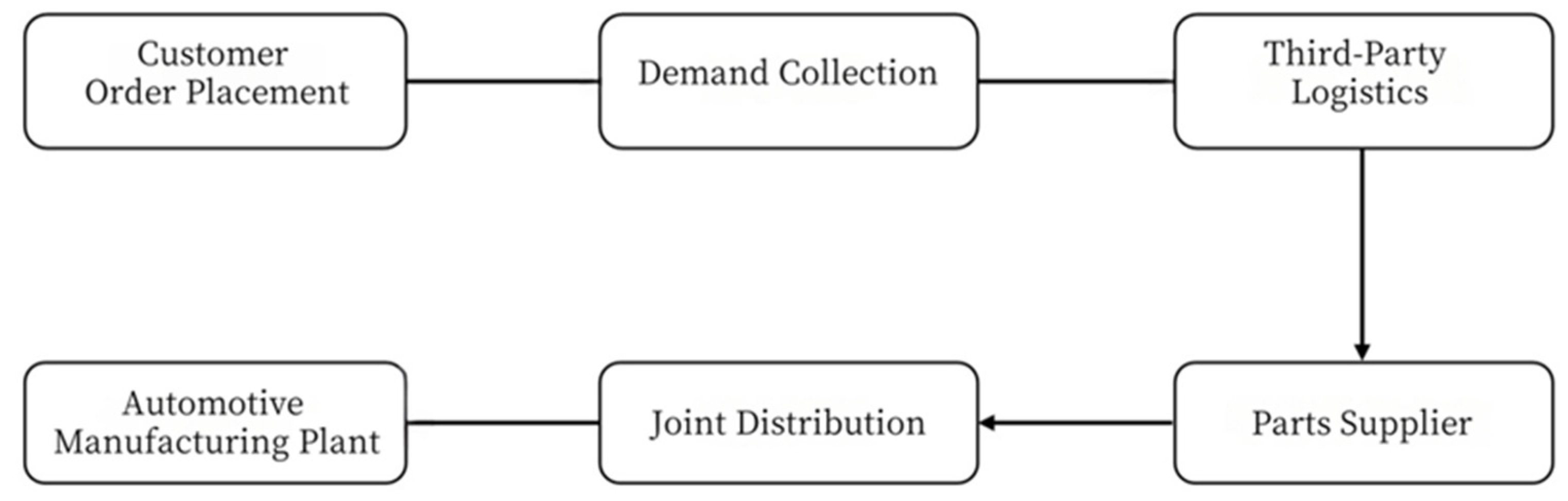
In the joint distribution process of multiple manufacturing plants, several automotive manufacturing plants share logistics resources, such as transportation and warehousing facilities, to optimize overall logistics efficiency and reduce costs. This model typically involves third-party logistics service providers, who coordinate the demands of different manufacturing plants to achieve efficient parts delivery. The distribution centers of multiple manufacturing plants quickly process the information and make decisions when they receive parts orders. Based on the order requirements and the geographic locations of the plants, the routes for joint distribution vehicles are optimized. Under a rolling replenishment policy with known lead times, the virtual distribution center is assumed to maintain adequate stock to support dispatching to multiple plants. This reflects an integrated inventory–routing approach, where replenishment orders are scheduled and synchronized with vehicle dispatch to mitigate stock-out risk and ensure reliable deliveries. The assumption is consistent with the modeling framework and practical considerations outlined in recent reviews of location–inventory–routing problems [52]. Delivery vehicles complete parts delivery to each plant within a specific timeframe, taking into account factors such as order demand, plant location, and time windows. Considering factors such as distance, time, and cost, the delivery vehicles return to the distribution center that offers the most significant cost reduction and wait for the next delivery instruction. The joint distribution process for multiple manufacturing plants is shown in Figure 1.

2.2. Description of the Joint Distribution Problem for Automotive Parts

This paper addresses the joint distribution routing problem for parts aimed at multiple automotive manufacturing plants. Specifically, within a specific region, multiple automotive manufacturers and parts suppliers are considered. The parts suppliers provide various parts to these automotive manufacturers, while third-party logistics companies offer joint distribution services for parts to multiple manufacturers. These logistics companies have multiple distribution centers, each equipped with a fleet of identical vehicles. Each supplier has an optimal service time window, and failure to pick up parts within the required time window incurs a penalty cost. Given that automotive manufacturers’ orders are usually placed in multiple batches, each being relatively small, third-party logistics companies should consider how to meet the changing demands of different manufacturers in each cycle while ensuring the lowest overall transportation cost. Under the joint distribution strategy for parts, multiple distribution centers jointly serve all automotive manufacturers in the region, while sharing demand resources and vehicle resources. This indicates that automotive manufacturers and vehicles are no longer fixed to a specific distribution center but are coordinated in space to minimize the delivery cost for each cycle. When planning the parts distribution routes, the following characteristics must be considered: First, the number of vehicles at each distribution center must meet the customer demands for each cycle. Second, the parts requirements of automotive manufacturers fluctuate across cycles, impacting the distribution center’s vehicle needs. Finally, upon completing deliveries, the vehicles return to the nearest distribution center, influencing the scheduling cost for subsequent cycles.

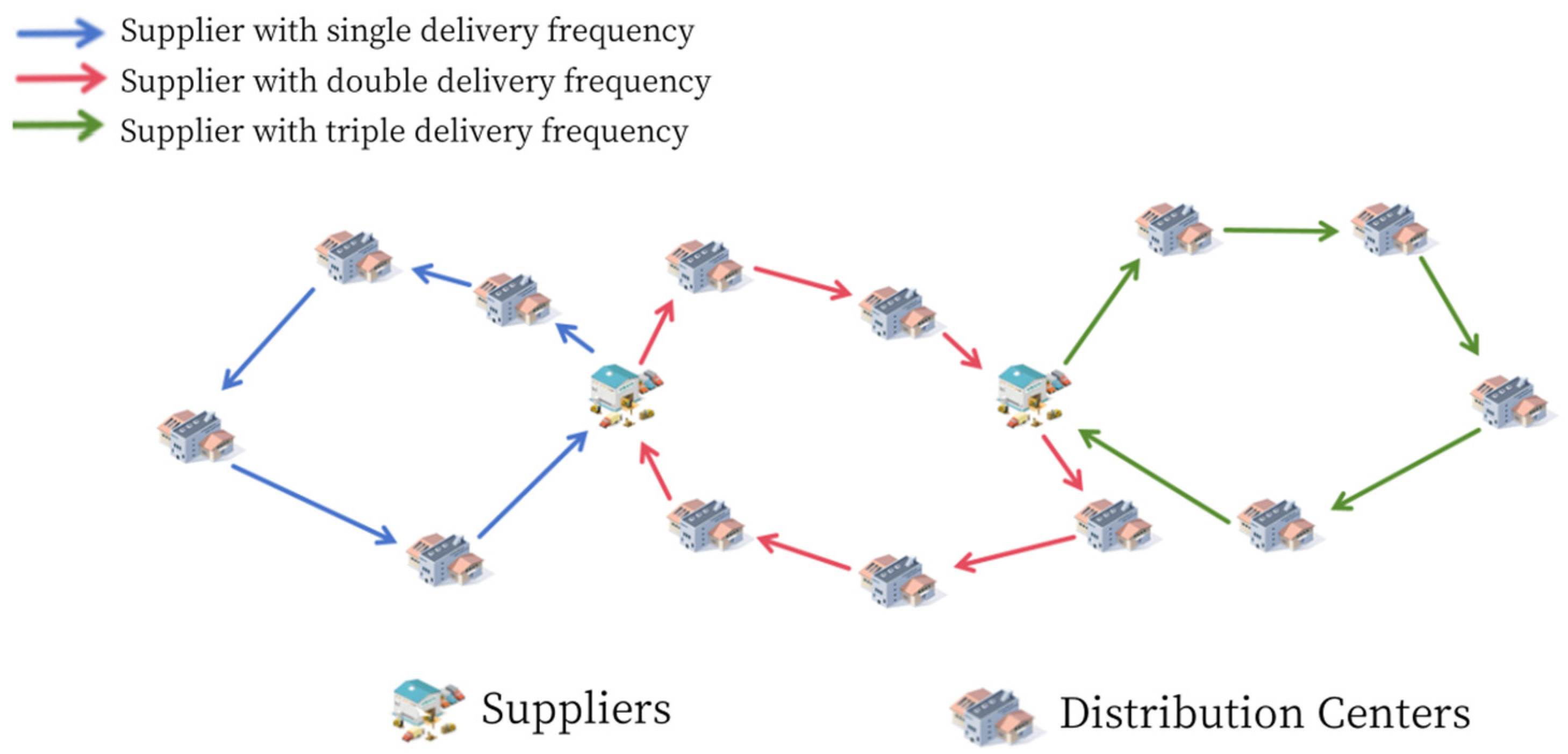
To further elucidate the joint distribution routing problem for parts serving multiple automotive manufacturing plants, Figure 2 presents a simplified example. The figure includes two collection and distribution centers and 13 parts suppliers. The collection and distribution centers are the core nodes of the logistics company, functioning to centralize the management and distribution of parts. Each parts supplier represents a source of parts for an automotive manufacturer, located at different geographical locations, involving varying service time windows and supply frequencies. The black nodes represent a supply frequency of once, the blue nodes represent a supply frequency of twice, and the yellow nodes represent a supply frequency of three times. In the parts distribution process, the third-party logistics company dispatches transportation vehicles from the collection and distribution centers. These transportation vehicles arrive at the corresponding suppliers within their service time windows to pick up parts. Upon completing the pickup, the vehicles return to any available collection and distribution center; they are not restricted to the original one. In this context, the central issue is to account for the service time windows and supply frequencies of different suppliers while efficiently planning and scheduling vehicle routes. This ensures that all pickup tasks are completed within the designated time windows and that automotive manufacturers’ parts demands are met, with the overarching goal of minimizing delivery costs and time. This constitutes the primary challenge addressed in this paper.

In the joint distribution path problem for parts serving multiple automotive manufacturers, third-party logistics companies should comprehensively consider the following optimization objectives to achieve the lowest total cost and fulfill customer orders:

Distribution Cost: In a highly competitive market, e-commerce and logistics companies rely on high-quality and satisfactory services to achieve profitability, with logistics delivery as a core service. Scientific planning of vehicle delivery schemes can substantially reduce logistics costs. Therefore, minimizing distribution costs is a crucial optimization objective.

Transportation Distance: The length of the transportation distance directly impacts the total distribution cost. Reasonably arranging vehicle delivery routes effectively reduces the travel distance, thereby minimizing the total delivery distance and curbing transportation costs. Thus, shortening transportation distance is one of the main optimization goals.

Delivery Time: In order to improve delivery efficiency and customer satisfaction, logistics delivery should meet customers’ high demands for timely delivery. Delays in delivery beyond the agreed time incur penalty costs proportional to the delay duration, thereby reducing customer satisfaction. Therefore, optimizing delivery time also emerges as an important goal.

Vehicle Quantity: The number of vehicles used to fulfill customer order deliveries also affects the delivery cost. An increase in the number of vehicles raises fixed costs, thereby increasing the total delivery cost. However, insufficient vehicle numbers may result in failure to meet customer demands and incur additional costs. Therefore, proper scheduling and capacity management are also essential optimization goals.

When planning the parts delivery paths, logistics companies should consider the service time windows and supply frequencies of different suppliers, as well as ways to complete all pickup tasks within different time windows. This will maximize the fulfillment of automotive manufacturers’ parts needs while minimizing delivery costs and time. This requires a comprehensive strategy that takes into account cost, efficiency, customer satisfaction, and service quality.

3. Model Construction

3.1. Basic Assumptions and Notations

The present research concentrates on exploring how to reasonably plan and schedule the transport vehicle routes while considering the service time windows and supply frequencies of suppliers. The core of the study lies in dynamically addressing the changing demands in each period while minimizing the total transportation cost. To clearly define the research problem and simplify the modeling process, the following assumptions are made in establishing the model for the joint distribution path problem of multiple automotive manufacturers:

(1)

The basic locations of parts suppliers and distribution centers are known;

(2)

Each parts supplier has an optimal service time window, and the logistics company must complete the pickup within this time window; otherwise, a penalty cost will be incurred;

(3)

The parts demand of each automotive manufacturer remains relatively stable during the study period, and the demand for each period can be predicted in advance;

(4)

Each distribution center has enough vehicles and resources to meet the demand of all automotive manufacturers, and the vehicle types and capacities are standardized and homogeneous;

(5)

In the joint distribution mode, vehicles can return to any distribution center upon completing the delivery task; they are not limited to the starting distribution center;

(6)

The distance between the automotive manufacturers and the parts distribution centers is ignored;

(7)

Multiple distribution centers can collaborate and share resources to meet the demand of all automotive manufacturers in the region;

(8)

Traffic conditions in the road network are ignored, and transport vehicles travel at a constant speed in the network;

(9)

Delivery costs are composed of fixed costs, which are determined by the number of vehicles, and variable costs, which are influenced by transportation distance and time.

The mathematical symbols used in the joint distribution model developed in this paper are summarized and explained in detail in

Table 1. Survey sample.

Symbol		Description Definition
Sets	$\mathrm{G}$	$\mathrm{Directed}\mathrm{network}\mathrm{graph},\mathrm{G}=\left(\mathrm{N},\mathrm{E}\right)$
	$\mathrm{N}$	$\mathrm{Node}\mathrm{set},\mathrm{including}\mathrm{the}\mathrm{supplier}\mathrm{set}\mathrm{and}\mathrm{the}\mathrm{automobile}\mathrm{manufacturer}\mathrm{set},\mathrm{N}=\mathrm{S}\cup \mathrm{P}=\left\{\mathrm{1,2},\dots ,\mathrm{n}+\mathrm{m}\right\}$
	$\mathrm{E}$	$\mathrm{Arc}\mathrm{set}\mathrm{between}\mathrm{nodes},\mathrm{E}=\left\{\left(\mathrm{i},\mathrm{j}\right)|\mathrm{i},\mathrm{j}\in \mathrm{N},\mathrm{i}\ne \mathrm{j}\right\}$
	$\mathrm{S}$	$\mathrm{Set}\mathrm{of}\mathrm{suppliers},\mathrm{S}=\left\{1,2,\dots ,\mathrm{n}\right\}$
	$\mathrm{P}$	$\mathrm{Set}\mathrm{of}\mathrm{automobile}\mathrm{manufacturers},\mathrm{P}=\left\{\mathrm{n}+1,\mathrm{n}+2,\dots ,\mathrm{n}+\mathrm{m}\right\}$
	$\mathrm{K}$	$\mathrm{Set}\mathrm{of}\mathrm{transport}\mathrm{vehicles}\mathrm{dispatched}\mathrm{by}\mathrm{the}\mathrm{third}\text{-}\mathrm{party}\mathrm{logistics}\mathrm{company},\mathrm{K}=\left\{\mathrm{1,2},\dots ,\mathrm{k}\right\}$
	$\mathrm{R}$	$\mathrm{Set}\mathrm{of}\mathrm{all}\mathrm{transport}\mathrm{vehicle}\mathrm{routes},\mathrm{R}=\left\{{\mathrm{r}}_1,{\mathrm{r}}_2,\dots ,{\mathrm{r}}_{\mathrm{n}}\right\}$
	$\mathrm{T}$	$\mathrm{Planning}\mathrm{cycle}\mathrm{for}\mathrm{cyclical}\mathrm{pickup},\mathrm{T}=\left\{1,2,\dots ,\mathrm{t}\right\}$
Parameters	${\mathrm{f}}_{\mathrm{j}\mathrm{k}}$	$\mathrm{Fixed}\mathrm{usage}\mathrm{cost}\mathrm{of}\mathrm{vehicle}\mathrm{k}$$\mathrm{at}\mathrm{distribution}\mathrm{center}\mathrm{j}$
	${\mathrm{c}}_{\mathrm{i}\mathrm{j}\mathrm{k}}$	$\mathrm{Driving}\mathrm{distance}\mathrm{cost}\mathrm{of}\mathrm{a}\mathrm{vehicle}\mathrm{from}\mathrm{node}\mathrm{i}$$\mathrm{to}\mathrm{node}\mathrm{j}$
	${\mathrm{p}}_{\mathrm{i}\mathrm{t}}$	$\mathrm{Penalty}\mathrm{cost}\mathrm{incurred}\mathrm{in}\mathrm{period}\mathrm{t}$$\mathrm{if}\mathrm{the}\mathrm{vehicle}\mathrm{fails}\mathrm{to}\mathrm{arrive}\mathrm{at}\mathrm{the}\mathrm{parts}\mathrm{supplier}\mathrm{i}\in \mathrm{S}$ within the service time window.
	${\mathrm{s}}_{\mathrm{j}\mathrm{t}}$	$\mathrm{Storage}\mathrm{cost}\mathrm{at}\mathrm{distribution}\mathrm{center}\mathrm{j}\in \mathrm{P}$$\mathrm{in}\mathrm{period}\mathrm{t}$.
	${\mathrm{q}}_{\mathrm{i}\mathrm{t}}$	$\mathrm{The}\mathrm{parts}\mathrm{supply}\mathrm{quantity}\mathrm{of}\mathrm{supplier}\mathrm{i}\in \mathrm{S}$$\mathrm{in}\mathrm{period}\mathrm{t}$
	${\mathrm{Q}}_{\mathrm{k}}$	The maximum load capacity of the transportation vehicle
	${\mathrm{D}}_{\mathrm{k}}$	$\mathrm{The}\mathrm{maximum}\mathrm{distance}\mathrm{for}\mathrm{vehicle}\mathrm{k}$ to return to the nearest distribution center
	${\mathrm{K}}_{\mathrm{j}\mathrm{t}}$	$\mathrm{The}\mathrm{vehicle}\mathrm{demand}\mathrm{at}\mathrm{distribution}\mathrm{center}\mathrm{j}$$\mathrm{in}\mathrm{period}\mathrm{t}$
	${\mathrm{c}}_{\mathrm{j}}$	$\mathrm{The}\mathrm{unit}\mathrm{storage}\mathrm{cost}\mathrm{at}\mathrm{distribution}\mathrm{center}\mathrm{j}$
	${\mathrm{e}}_{\mathrm{i}}$	$\mathrm{The}\mathrm{earliest}\mathrm{time}\mathrm{point}\mathrm{at}\mathrm{which}\mathrm{supplier}\mathrm{i}$ accepts pickup services
	${\mathrm{l}}_{\mathrm{i}}$	$\mathrm{The}\mathrm{latest}\mathrm{time}\mathrm{point}\mathrm{at}\mathrm{which}\mathrm{supplier}\mathrm{i}$ accepts pickup services
	${\mathrm{s}\mathrm{t}}_{\mathrm{i}\mathrm{t}}$	$\mathrm{The}\mathrm{service}\mathrm{start}\mathrm{time}\mathrm{of}\mathrm{supplier}\mathrm{node}\mathrm{i}$$\mathrm{in}\mathrm{planning}\mathrm{period}\mathrm{t}$
	${\mathrm{s}}_{\mathrm{i}}$	$\mathrm{The}\mathrm{time}\mathrm{required}\mathrm{to}\mathrm{complete}\mathrm{the}\mathrm{pickup}\mathrm{service}\mathrm{at}\mathrm{supplier}\mathrm{node}\mathrm{i}$
	$\mathrm{M}$	A sufficiently large constant
	${\mathrm{S}\mathrm{m}}_{\mathrm{i}}$	$\mathrm{The}\mathrm{minimum}\mathrm{visit}\mathrm{frequency}\mathrm{for}\mathrm{supplier}\mathrm{i}$ to accept the pickup service
	${\mathrm{F}}_{\mathrm{i}}$	$\mathrm{The}\mathrm{pickup}\mathrm{frequency}\mathrm{of}\mathrm{supplier}\mathrm{i}$
Variables	${\mathrm{x}}_{\mathrm{i}\mathrm{j}\mathrm{k}\mathrm{t}}$	$\mathrm{A}0\text{-}1\mathrm{variable},\mathrm{where}\mathrm{it}\mathrm{is}1\mathrm{if}\mathrm{vehicle}\mathrm{k}$$\mathrm{departs}\mathrm{from}\mathrm{node}\mathrm{i}$$\mathrm{and}\mathrm{arrives}\mathrm{at}\mathrm{node}\mathrm{j}$$\mathrm{in}\mathrm{period}\mathrm{t}$ and 0 otherwise
	${\mathrm{z}}_{\mathrm{j}\mathrm{k}\mathrm{t}}$	$\mathrm{A}0\text{-}1\mathrm{variable},\mathrm{where}\mathrm{it}\mathrm{is}1\mathrm{if}\mathrm{vehicle}\mathrm{k}$$\mathrm{returns}\mathrm{to}\mathrm{distribution}\mathrm{center}\mathrm{j}$$\mathrm{in}\mathrm{period}\mathrm{t}$ and 0 otherwise
	${\mathrm{u}}_{\mathrm{i}\mathrm{j}\mathrm{k}\mathrm{t}}$	$\mathrm{A}\mathrm{continuous}\mathrm{variable}\mathrm{representing}\mathrm{the}\mathrm{load}\mathrm{of}\mathrm{vehicle}\mathrm{k}$$\mathrm{from}\mathrm{distribution}\mathrm{center}\mathrm{j}$$\mathrm{to}\mathrm{parts}\mathrm{supplier}\mathrm{i}$$\mathrm{in}\mathrm{period}\mathrm{t}$
	${\mathrm{w}}_{\mathrm{i}\mathrm{j}\mathrm{k}\mathrm{t}}$	$\mathrm{A}\mathrm{continuous}\mathrm{variable}\mathrm{representing}\mathrm{the}\mathrm{waiting}\mathrm{time}\mathrm{of}\mathrm{vehicle}\mathrm{k}$$\mathrm{from}\mathrm{distribution}\mathrm{center}\mathrm{j}$$\mathrm{to}\mathrm{parts}\mathrm{supplier}\mathrm{i}$$\mathrm{in}\mathrm{period}\mathrm{t}$

.

3.2. Model Formulation

The model constructed in this study for the joint distribution path problem of automotive parts, incorporating multi-manufacturer collaboration, is designed to minimize the total operational cost within the multi-manufacturer collaborative delivery system. The objective function of this model comprises four main components of cost: inherent cost of dispatching transportation vehicles, cost of vehicle travel distance, penalty cost for failing to meet the supplier’s service time window, and storage cost incurred by the supplier during the waiting period.

(1)

Vehicle Fixed Cost

In the multi-manufacturer collaborative automotive parts joint distribution path optimization model, the fixed cost of transportation vehicles usually refers to costs related to the purchase, maintenance, insurance, and depreciation of the vehicles. These costs are fixed at the time of vehicle purchase and remain constant throughout the vehicle’s operational period, independent of usage frequency or travel distance. In this section, the fixed cost of transportation vehicles is represented as

$$Z_1=\sum _{i\in N}\sum _{j\in N}\sum _{k\in K}\sum _{t\in T}{f}_{jk}·x_{ijkt}$$

(1)

(2)

Vehicle Travel Distance Cost

Vehicle travel distance cost represents the cost accumulated linearly based on the vehicle’s travel distance during the delivery process. This cost reflects the marginal cost of vehicle operation. Herein, it is assumed that the vehicles maintain a constant speed throughout the delivery process, without considering acceleration or deceleration. Therefore, the vehicle’s travel distance cost is directly proportional to the distance traveled; the longer the distance, the higher the associated cost. The vehicle travel distance cost can be expressed as

$$Z_2=\sum _{i\in N}\sum _{j\in N}\sum _{t\in T}\sum _{k\in K}{c}_{ijk}·x_{ijkt}$$

(2)

(3)

Penalty Cost

Penalty cost arises when deliveries are not completed within the supplier’s specified time window. This cost is typically introduced to compensate for potential disruptions and losses in the supply chain caused by delivery delays. The inclusion of penalty costs aims to ensure the timeliness of the distribution plan, thereby encouraging logistics companies to adhere to suppliers’ time constraints when planning delivery routes and scheduling vehicles. This facilitates maintenance of the stability and efficiency of the entire supply chain. The penalty cost can be expressed as

$$Z_3=\sum _{i\in S}\sum _{t\in T}{p}_{it}$$

(3)

(4)

Storage Cost

Storage cost refers to the expenses incurred by suppliers while waiting for delivery. This typically includes warehouse storage fees, rental costs, insurance, and expenses related to maintaining storage conditions (such as temperature and humidity control). In the optimization model, incorporating storage costs is crucial for developing an effective distribution strategy, given its direct influence on overall logistics costs. Minimizing storage costs minimizes capital occupation in the supply chain and potential losses, thereby enhancing its overall economic efficiency. The storage cost can be expressed as

$$Z_4=\sum _{j\in }\sum _{t\in T}{s}_{jt}$$

(4)

Overall, the objective function of this study can be expressed as follows:

$$\mathit{min}\left[Z_1+Z_2+Z_3+Z_4\right]$$

(5)

Constraints:

$$\sum _{j\in N}\sum _{k\in K}{u}_{ijkt}\ge q_{it},\forall i\in N,t\in T$$

(6)

$$\sum _{i\in S}{x}_{ijkt}·q_{it}\le Q_k,\forall j\in S,i\ne j,\forall k\in K,\forall t\in T$$

(7)

$$\sum _{j\in S}{x}_{ijkt}\le 1,\forall i\in S,i\ne j,\forall k\in K,\forall t\in T$$

(8)

$$\sum _{k\in K}{x}_{ijkt}\ge K_{jt},\forall i\in S,\forall j\in P,\forall t\in T$$

(9)

$$\sum _{i\in S}\sum _{k\in K}{x}_{ijkt}\ge 1,\forall j\in P,\forall t\in T$$

(10)

$$s{t}_{it}\ge e_i,\forall t\in T,\forall i\in S$$

(11)

$$s{t}_{it}+s_i\le l_i,\forall t\in T,\forall i\in S$$

(12)

$$s{t}_{it}+s_i+w_{ijkt}+t_{ij}\le s{t}_{jt},\forall t\in T,\forall i\in S,\forall j\in S,\forall k\in K$$

(13)

$$\sum _{t\in T}{x}_{ijkt}=F_i,\forall i\in S,j\in S,\forall k\in K$$

(14)

$$\sum _{i\in S}{x}_{ijkt}·d_{ij}\le D_k,\forall j\in P,\forall k\in K,\forall t\in T$$

(15)

$$s_{jt}\ge c_j·(1-\sum _{i\in S}\sum _{k\in K}{x}_{ijkt}),\forall j\in P,\forall t\in T$$

(16)

$$z_{jkt}\ge x_{ijkt},\forall i\in S,\forall j\in P,\forall k\in K,\forall t\in T$$

(17)

$$\sum _{i\in S}{x}_{ijkt}-\sum _{i\in S}{x}_{ijk\left(t+1\right)}=0,\forall j\in S,\forall k\in K,\forall t\in T$$

(18)

$$u_{ijkt}\le M·x_{ijkt},\forall i,j\in S,\forall k\in K,\forall t\in T$$

(19)

$$u_{ijkt}-u_{ijk\left(t+1\right)}=0,\forall i,j\in N,\forall k\in K,\forall t\in T$$

(20)

$$\sum _{i\in S}\sum _{k\in K}{u}_{ijkt}=\sum _{i\in S}{q}_{it},\forall j\in P,\forall t\in T$$

(21)

$$\sum _{i\in S}\sum _{t\in T}{x}_{ijkt}\ge S{m}_i,\forall j\in P,\forall k\in K$$

(22)

Constraints include time window constraints, vehicle resource constraints, demand variation constraints, and vehicle scheduling cost constraints. Among them, Equation (6) ensures that the pickup volume of each parts supplier is satisfied in each cycle; Equation (7) ensures that the pickup volume of vehicles at each supplier does not exceed their maximum load capacity; Equation(8) ensures that each transport vehicle serves each supplier at most once per cycle; Equation (9) restricts the number of vehicles at each distribution center to meet the pickup demand of suppliers in each cycle; Equation (10) ensures that at least one transport vehicle departs from each distribution center in each cycle; Equations (11) and (12) ensure that vehicle pickup services are performed within the suppliers’ specified time windows; Equation (13) constrains the continuity of pickup service time, waiting time, and travel time of transport vehicles; Equation (14) ensures that the pickup frequency of transport vehicles at each parts supplier complies with the predetermined frequency; Equation (15) ensures that transport vehicles return to the nearest distribution center after completing delivery tasks; Equation (16) stipulates that storage costs are incurred if distribution center vehicles are not utilized; Equation (17) ensures that transport vehicles return to the distribution center by the end of each cycle; Equation (18) ensures the balance of transport vehicle usage across consecutive cycles; Equation (19) ensures the positive correlation between vehicle loading and route; Equation (20) ensures the continuity of vehicle loading across consecutive cycles; Equation (21) ensures that the total pickup volume at distribution centers equals the total supply volume of all parts suppliers; and Equation (22) ensures that the utilization rate of each transport vehicle meets or exceeds the specified minimum threshold.

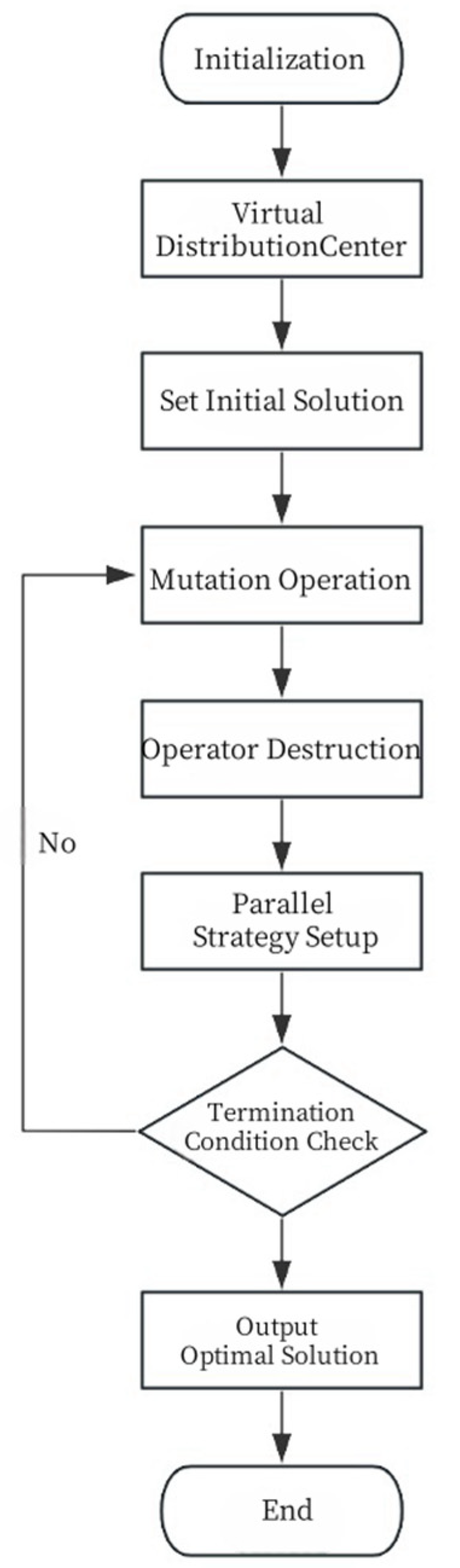
4. Solution Algorithm

This study primarily addresses the optimization of joint distribution routes for automotive parts in a multi-manufacturer collaboration scenario. The core challenge lies in efficiently meeting the supply demands of various parts suppliers while ensuring that distribution vehicles return to their original distribution centers upon completing their tasks. Currently, there are two common methods for solving this optimization problem:

Fixed Service Area Method: This method assigns a fixed service area to each distribution center, ensuring that they operate relatively independently. Despite its ease of implementation and management, this approach may lead to an uneven distribution of customers among centers due to improper area division, potentially resulting in local optima.

Virtual Distribution Center Method: This method incorporates a virtual distribution center, where all vehicles are assumed to originate from and return to a single hub. By transforming a multi-depot vehicle routing problem into a single-depot problem, it enables more effective global route planning and improves resource integration across distribution centers. The introduction of a virtual distribution center allows for enhanced flexibility in vehicle dispatching, preventing resource waste and suboptimal solutions caused by rigid service area assignments.

In summary, this study proposes an innovative solution framework by integrating the virtual distribution center approach with an improved variable neighborhood search (PIVNS) algorithm to optimize the joint distribution routes of automotive parts. First, the original multi-manufacturer parts distribution problem is transformed into a cyclic pickup routing problem with a virtual distribution center, simplifying its complexity by ensuring that all vehicles start and return to a single center, thereby reducing the problem’s computational difficulty. To enhance computational feasibility and focus on the core mechanism of multi-manufacturer coordination, the model assumes constant vehicle speeds and fixed vehicle capacities. These simplifications are common in urban logistics optimization and do not compromise result validity, as they reflect stable operational conditions frequently found in structured distribution scenarios. Second, an improved variable neighborhood search algorithm (PIVNS) is proposed to address the transformed problem, leveraging parallel computing for computational efficiency enhancement. The primary steps involve initialization, parameter determination, iterative operator updates, and parallel processing. The overall workflow is illustrated in Figure 3.

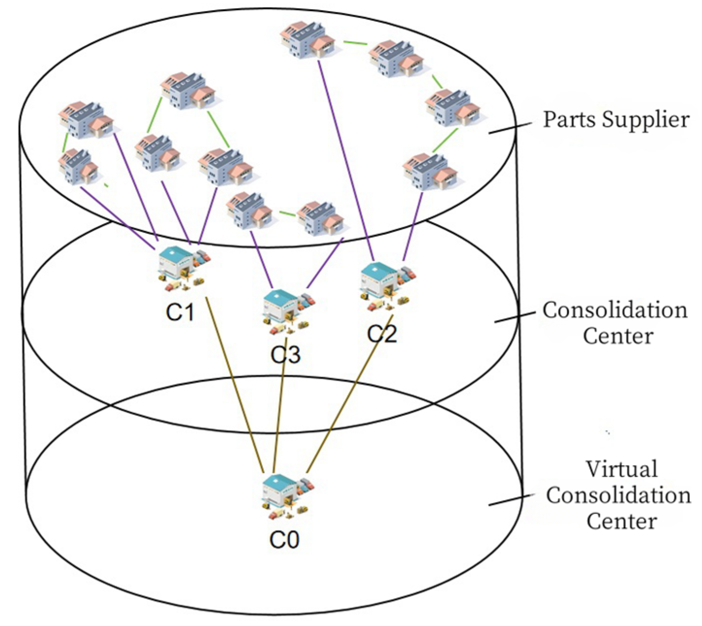
4.1. Virtual Distribution Center Construction

In the context of optimizing joint distribution routes for automotive parts under multi-manufacturer collaboration, the establishment of a virtual distribution center is essential for reducing problem complexity and promoting resource sharing. Basic steps for constructing the virtual distribution center are as follows:

• Step 1: Definition of Virtual Distribution Center

A virtual geographic location is designated as the starting and ending point for all distribution vehicles. This location functions as a logical consolidation hub and does not require a physical presence.

• Step 2: Resource Integration

All vehicle resources from actual distribution centers are consolidated into the virtual distribution center. In this model, all vehicles are considered to depart from the virtual distribution center, complete their delivery tasks, and then return to the virtual center.

• Step 3: Establishment of Mapping Between the Virtual and Actual Distribution Centers

Each actual distribution center and automotive manufacturer is linked to the virtual center, with their respective distances and relative positions determined.

• Step 4: Vehicle Dispatching and Route Planning

All vehicles are dispatched from the virtual center and return to it upon completion of their tasks. This transformation simplifies the problem into a single-center routing issue originating from the virtual distribution center, reducing overall complexity.

• Step 5: Service Time Window of the Virtual Center

The service time window for the virtual center is determined based on the demand of each distribution center, the automotive manufacturers, and the suppliers’ service time windows, thereby facilitating the scheduling of vehicle departures to satisfy all time constraints.

To further understand, Figure 3 presents a simple example of the virtual center setup. In Figure 4, $c_1$, $c_2$, and $c_3$ represent the parts distribution centers, and $c_4$—$c_{14}$ represent the parts suppliers. In this context, a virtual distribution center $c_0$ is established, with the distance between the virtual center and the actual distribution center set as zero, and the distance from all parts suppliers to the virtual center is set as ∞. Each transportation vehicle departs from the virtual distribution center and passes through an actual distribution center to reach the parts supplier. Upon delivery completion, the vehicle returns through an actual distribution center back to the virtual center, while ensuring that its load capacity limit is not exceeded. Importantly, the introduction of the virtual distribution center does not alter the adherence to all other constraints associated with multi-manufacturer collaborative parts distribution.

4.2. Initial Solution Setup

To summarize, the changes in parking demand over time are different for different types of land use, each with its own unique trend in parking demand. The average parking demand rates of the three different types of land use are compared horizontally, and the length of the shaded area qualitatively characterizes the size of the parking demand rate, as shown in Figure 2.

In the IVNS algorithm, a feasible solution sss represents a set of the sequence of parts supplier nodes visited by delivery vehicles. The algorithm framework is as follows:

Step 1: Generate the initial solution sss and initialize the parameters, including maximum random destruction percentage rand_d_max, minimum random destruction percentage rand_d_min, maximum worst destruction percentage worst_d_max, minimum worst destruction percentage worst_d_min, number of regret-based repair operators in suboptimal positions regret_n, initial temperature for simulated annealing T0, cooling coefficient μ, minimum temperature Tf, maximum iteration count max_iter, weights of all destruction and repair operators wi, scores of the operators πi, reward of the operators α, interval iteration count for adjusting operator weights δ, and operator weight inheritance coefficient η.

Step 2: Calculate the weights of the operators according to their scores and employ the roulette method to select the destruction and repair operators. These operators are then applied to the current solution to generate a new solution sts_tst.

Step 3: Apply the acceptance criterion of simulated annealing (SA) to determine whether to accept the current solution sts_tst.

Step 4: Update the scores of all operators following the adaptive layer operator score updating method and then update the temperature of simulated annealing.

Step 5: Upon every δ\deltaδ iteration, update the weights of all operators and reset the temperature of simulated annealing.

Step 6: Repeat Steps 2 to 5 until the termination condition of the iteration is met.

4.3. Mutation Operation

In genetic algorithms, mutation operation refers to the process of introducing random changes in the genetic makeup of individuals. Its primary function is to maintain population diversity and prevent the algorithm from getting trapped in local optima. Mutation serves as a vital genetic operator, maintaining population genetic diversity and enhancing the algorithm’s ability to explore the search space in pursuit of superior solutions. Following natural selection and crossover operations, the population may tend to become homogeneous, potentially causing the algorithm to get stuck in a local optimum instead of reaching a global optimum. By introducing new genetic mutations, the algorithm is prompted to escape from local optima and explore new possibilities. Mutation represents an indispensable part of genetic algorithms, operating alongside selection and crossover operations to drive the algorithm toward a global optimum. In practical applications, mutation probability is typically set within a lower range to ensure that the existing good genetic combinations are not overly disrupted while still effectively exploring new possibilities. Common mutation methods in genetic algorithms include the following:

Bit-flip Mutation: Randomly select one or more loci on the chromosome and flip their values, suitable for binary-coded chromosomes.

Random Reset Mutation: Randomly assign a new value to one or more genes on the chromosome, suitable for chromosomes with finite set encoding.

Swap Mutation: Randomly select two loci on the chromosome and swap their values, suitable for permutation-coded chromosomes.

Insert Mutation: Randomly select a locus on the chromosome and move it to another position, suitable for permutation-coded chromosomes.

Reversal Mutation: Randomly select a segment of the chromosome and reverse the order of genes within that segment, suitable for permutation-coded chromosomes.

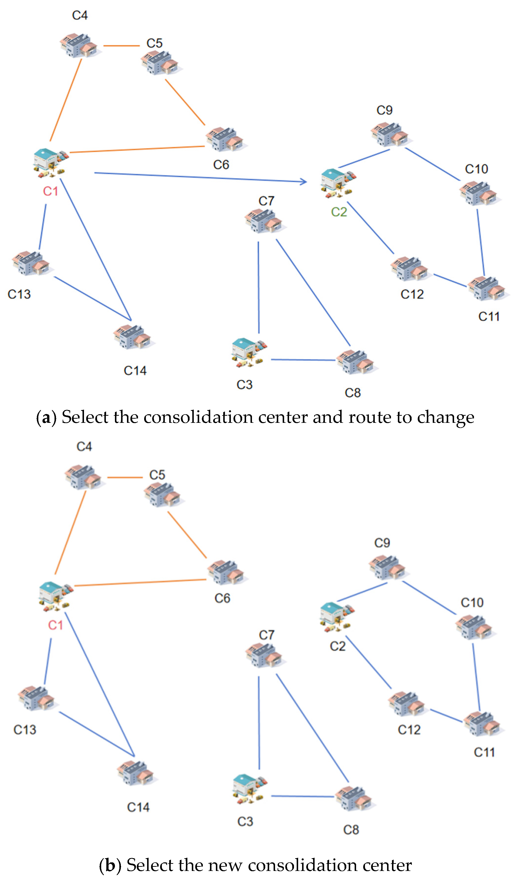
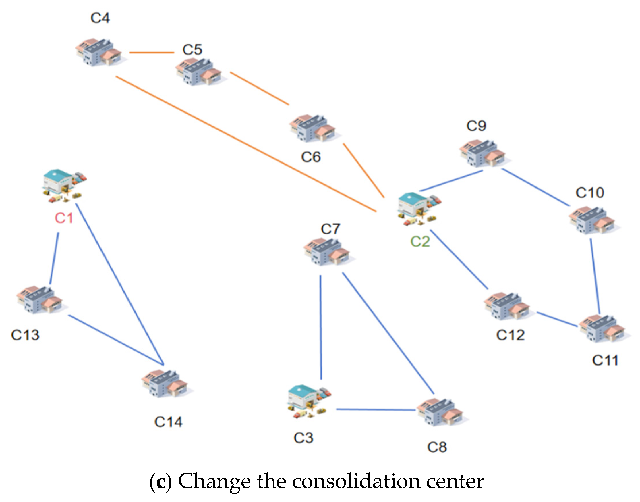
Drawing on the mechanism of mutation operations in genetic algorithms, this study further applies it to the VNS algorithm to facilitate the discovery of more potential solutions in the search space. Two mutation operations are correspondingly proposed, which can generate new solutions without significantly deviating from the original solution. Specifically, the first mutation operation involves adjusting the collection and distribution centers along the route, while the second alters the component suppliers along the route. Figure 5 illustrates a simple example of the collection and distribution center mutation operation. As shown in the figure, the mutation operation on the collection and distribution center first involves selecting a collection and distribution center and a route, such as A and B (Figure 5a). Subsequently, a new collection and distribution center is selected (Figure 5b), and by changing the first selected collection and distribution center to the second one, a new solution is accordingly generated (Figure 5c).

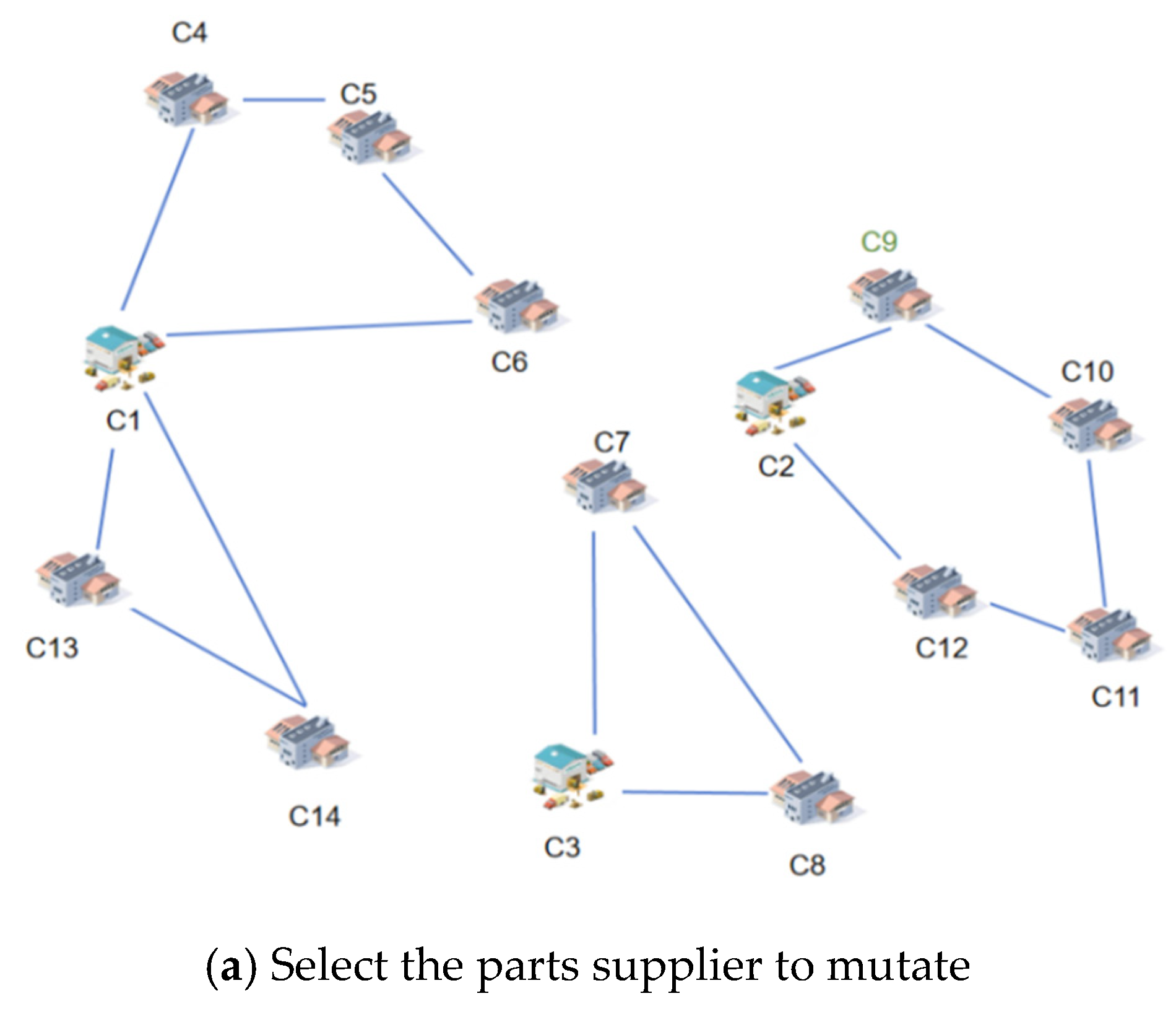
The mutation operation for component suppliers is illustrated in Figure 6. Consistent with the mutation operation for adjusting collection and distribution centers, the mutation for component suppliers initiates with the selection of a specific component supplier, such as c9 (Figure 6a). Following that, the two edges connected to the selected component supplier are removed. These two edges, which are associated with the selected supplier, are deleted, and other suppliers or collection centers connected to the deleted edges are directly reconnected. Subsequently, a route passing through any collection and distribution center, such as B, is selected. By linking the selected component supplier with the last supplier and the collection and distribution center on the selected route, a new solution is generated, as shown in Figure 6b. Given that the newly selected component supplier is inserted directly between the last supplier and the collection and distribution center, it may disrupt the local optimality of the new route. Therefore, to ensure the local optimality of each route in the new solution, a 2-opt exchange is conducted by evaluating all possible pairwise exchanges of supplier positions within the route. The mutated route is depicted in Figure 6c.

4.4. Operator Destruction and Repair

As mentioned previously, the IVNS algorithm is fundamentally based on solution destruction and repair, dynamic weight adjustment, and adaptive selection. Through the development of multiple destruction and repair operators, the search space for solutions is expanded, and the current solution is improved. Destruction and repair methods with superior performance are assigned higher scores and correspondingly higher weights. In each iteration, the selection and weight adjustment of these operators are determined based on their previous performance, using efficient combination methods to enhance the algorithm’s optimization capability and ultimately identify the optimal solution.

Each destruction and repair operator i has a score πi, which is initially set to zero. During the iteration process, the score is updated based on the quality of the newly generated solution, as detailed below:

$${\pi }_i=\left\{\begin{array}{c}{\pi }_i+{\alpha }_1,ifthenewsolutionisbetterthanthecurrentbestsolution;\\ {\pi }_i+{\alpha }_2,ifthenewsolutionisbetterthanthecurrentsolution;\\ {\pi }_i+{\alpha }_3,ifthenewsolutionisworsethanthecurrentsolution,butaccepted;\\ {\pi }_i,ifthenewsolutionisnotaccepted.\end{array}\right.$$

(23)

where${\alpha }_1$, ${\alpha }_2$, and ${\alpha }_3$ represent the reward scores of the operators. The weights of the operators are periodically updated every $\delta$ iterations based on their respective scores.

Each destruction and repair operator $i$ is assigned a weight ${\omega }_i$, which is initially set to 1 and updated during the iterations based on the operator’s performance scores, as detailed below:

$${\omega }_i=\left\{\begin{array}{c}{\omega }_i+(1-\eta ){\displaystyle \frac{{\pi }_i}{{\theta }_i}},{\theta }_i>0\\ \eta {\omega }_i,{\theta }_i=0.\end{array}\right.$$

(24)

where $\eta \in \left(\mathrm{0,1}\right)$ represents the inheritance coefficient for the operator’s previous weight, and ${\theta }_i$ denotes the number of times operator $i$ was selected in the previous $\delta$ iterations.

4.5. Parallel Computing Strategy

The IVNS algorithm involves significant computation. To improve efficiency, parallel computing strategies should necessarily be adopted. The main strategies for IVNS include the following four:

Independent Strategy: Each processor or computational node runs an independent VNS instance. Each instance applies different initial solutions or varying neighborhood structure sequences for searching. No information exchange exists between instances, and each independently explores the solution space. This strategy is simple to implement and easy to parallelize. Each processor focuses solely on its own VNS search process without complex communication mechanisms. However, due to the lack of information exchange, different instances may repeatedly explore similar areas during the search, limiting the efficiency improvement and possibly failing to fully exploit the collaborative advantage of multiple processors.

Master–Slave Strategy: A master node is set up as the “master VNS,” serving to collect and update global information, such as recording the best solution found by each slave node. Other nodes act as “slave VNSs” and execute the specific search tasks. During the search process, each slave VNS periodically sends its results to the master VNS, which updates global information, such as the global optimal solution. The master VNS then provides this updated information back to the slave VNS, which adjusts its search strategy (e.g., changing the order of neighborhood structure selection) based on the global information. This strategy allows for global information sharing and coordination, enabling each slave VNS to adjust its search direction and thus improve the search efficiency and solution quality. However, the master VNS becomes a communication and information-processing bottleneck, possibly limiting the overall performance. Additionally, the delay in information transmission may impact the timely response of the slave VNS to global information.

Fine-Grained Strategy: The solution space is divided into multiple smaller subspaces, each of which is assigned to a processor or computational node for search operations. Within the same subspace, processors can exchange information, including the efficacy of neighborhood structures and local optimal solutions, to collaboratively enhance the search optimization within that subspace. Communication between processors in different subspaces is limited to reduce communication overhead. This strategy is particularly well-suited for large-scale problems, as it fully utilizes parallel computing resources to search multiple subspaces simultaneously, thereby improving search efficiency. Information exchange within the same subspace accelerates local optimization. However, the correct design of subspace partitioning is crucial to ensure that each subspace has enough solution space for searching, and the boundary handling between subspaces can be complex. Furthermore, the isolation of subspaces may limit the search for global optimal solutions.

Coarse-Grained Strategy: The solution space is divided into several larger regions, with one or more processors in each region responsible for conducting the VNS search. Processors within the same computational group collaborate to search within the region, sharing strategies such as the use of neighborhood structures or search paths. Communication between different computational groups focuses primarily on updating and sharing the global optimal solution, with periodic exchanges of the best solutions found by each group to promote global search progress. This strategy facilitates parallel search on a larger scale, thereby reducing communication frequency between processors and minimizing communication overhead. Intra-group collaboration helps dig deeper into the quality solutions within the large region, while inter-group exchanges ensure the effectiveness of the global search. However, partitioning the solution space into large regions and forming computational groups requires consideration of problem scale and processor number. Improper partitioning may lead to an imbalanced search. Additionally, limited information exchange between computational groups may hinder the timely dissemination of global information.

In this study, the improved VNS algorithm is expected to be implemented in a distributed environment rather than share the same memory system. If the algorithm involves significant communication between processors, the parallel effect will be significantly reduced. Therefore, a parallel strategy with low communication costs should necessarily be adopted. The coarse-grained strategy, due to its low communication requirements, can speed up convergence while ensuring the solution quality, making it well-suited for use in a distributed environment. The coarse-grained strategy involves exchanging information between processors within a group at specific intervals or after a certain number of iterations, typically involving the utilization of a ring topology to facilitate this exchange. By exchanging high-quality solutions, the solution space can be diversified, effectively preventing premature convergence.

In the VNS algorithm, the parallel implementation of the coarse-grained strategy involves multiple processors, and the information exchange between them typically occurs at certain iteration intervals or after a specific number of iterations. To effectively prevent premature convergence, various topologies, such as the ring topology, can be employed. In the ring topology, each processor exchanges information with its adjacent processors. This approach diversifies the solution space across processors, thereby reducing the risk of local optima and enhancing the algorithm’s global search ability.

Recent evidence strongly supports the efficacy of coarse-grained (island-model) parallelization in metaheuristic algorithms. The latest survey by Crainic et al. underscores that island strategies offer superior scalability and maintain robust solution quality in distributed computing environments [53]. Similarly, a study by Smith & Patel demonstrated that coarse-grained parallel VNS for VRPs achieves faster convergence and lower communication overhead compared to fine-grained alternatives [54]. These findings substantiate our choice of coarse-grained parallelism as both practical and efficient in distributed logistics optimization contexts.

Although commercial solvers such as CPLEX and Gurobi are widely used to solve standard VRP variants, they often struggle with scalability and inflexibility when applied to large-scale, multi-depot problems involving collaboration constraints. In contrast, metaheuristic methods—especially parallel VNS—offer greater adaptability and runtime efficiency. Recent comparative studies substantiate this choice. Arenas-Vasco et al. showed that a combined metaheuristic significantly outperformed Gurobi in solving periodic capacitated multi-depot VRP instances, achieving comparable solution quality in much less time [55]. Wang et al. demonstrated that coarse-grained parallel VNS outperformed CPLEX on large-scale collaborative routing problems, in both accuracy and speed [56]. These findings support the practical decision to employ PIVNS as a scalable, efficient, and flexible optimization tool for complex collaborative logistics scenarios in this study.

To further explore the environmental significance of the proposed V-MDVRP model, a preliminary estimation of carbon emission reductions was conducted. Based on prior studies [1], the average carbon emission per kilometer of freight transport is approximately 0.27 kg CO₂/km. Using this coefficient, the total emission difference between the best- and worst-performing distribution scenarios is estimated to be around 73.85 kg CO₂. This indicates that the collaborative optimization model not only enhances economic efficiency but also contributes to sustainable logistics by lowering environmental impact.

5. Case Study Analysis

The multi-manufacturer collaborative automotive parts joint distribution route problem model constructed in this study presents a new problem. A review and analysis of the existing literature reveals that no directly applicable example exists for the problem discussed in this paper. Therefore, in order to evaluate the effectiveness of the proposed PIVNS algorithm and model, this study selects relevant example data from the literature, modifies certain information such as service time, and conducts numerical experiments. The implementation of the PIVNS algorithm is carried out using Python 3.9.7.

The selected example data for this study includes two automotive manufacturers (i.e., two collection centers) and 21 automotive parts suppliers. The suppliers are further divided into three periods for parts supply, each having its own service time and supply volume. Some suppliers do not provide services. The specific information of the collection centers and suppliers is shown in Table 2 and Table 3.

Table 2. Data information of the distribution center.

Number	Node	X-Coordinate	Y-Coordinate
1	Distribution Center 1	36.163	52.559
2	Distribution Center 2	−41.387	−8.105

Table 2. Data information of the distribution center.

Number	Node	X-Coordinate	Y-Coordinate
1	Distribution Center 1	36.163	52.559
2	Distribution Center 2	−41.387	−8.105

Table 3. Data information of part suppliers.

Supplier ID	X-Coordinate	Y-Coordinate	First Period		Second Period		Third Period		Earliest Service Time	Latest Service Time
			Service Time (s)	Pickup Quantity	Service Time (s)	Pickup Quantity	Service Time (s)	Pickup Quantity
1	77.52	51.63	20	6.7	14	0	21	2.4	399	525
2	−4.6	−34.35	13	4.3	22	7.5	16	5.4	399	525
3	19.87	−31.46	12	3.9	18	2.8	21	2.7	121	299
4	−68.55	−84.13	19	3	16	5.4	22	4.4	389	483
5	−22.18	−14.34	17	1.8	14	1.6	13	1	204	304
6	81.34	41.85	17	5.8	14	1.4	13	4.4	317	458
7	14.52	−67.5	12	4	19	6.4	13	1.3	160	257
8	−77.85	−64.66	13	1	15	1.8	18	6.2	170	287
9	−19.39	68.6	17	7.7	12	4	11	3.7	215	321
10	−33.49	−99.13	16	2.2	15	3.8	15	1.8	80	233
11	−38.51	88.88	22	7.4	18	2.9	17	2.4	90	206
12	−93.89	−63.72	18	6.3	21	7	23	7.9	397	525
13	52.75	−79.73	20	6.7	15	1.9	13	1.2	271	420
14	−62.25	60.74	10	3.5	20	6.8	16	2	108	266
15	69.23	49.1	19	3.2	10	3.5	16	2.2	340	462
16	65	−95.8	18	6	17	5.8	23	7.1	226	377
17	58.62	−51.88	16	2.1	16	5.4	14	1.5	446	604
18	−22.39	84.47	18	6.1	18	2.6	18	3.6	444	566
19	63.99	−7.01	21	7.3	10	3.3	16	5.4	319	460
20	−66.89	16.37	14	1.3	15	4.7	14	1.6	192	312
21	−90.46	−46.97	18	6	12	4	17	5.7	65	462

The number of automotive manufacturers and collection centers is equal, both being two. The parameters for each delivery vehicle are maintained consistently. The key parameters configuration for the PIVNS algorithm is shown in Table 4, below.

Table 3. Data information of part suppliers.

Supplier ID	X-Coordinate	Y-Coordinate	First Period		Second Period		Third Period		Earliest Service Time	Latest Service Time
			Service Time (s)	Pickup Quantity	Service Time (s)	Pickup Quantity	Service Time (s)	Pickup Quantity
1	77.52	51.63	20	6.7	14	0	21	2.4	399	525
2	−4.6	−34.35	13	4.3	22	7.5	16	5.4	399	525
3	19.87	−31.46	12	3.9	18	2.8	21	2.7	121	299
4	−68.55	−84.13	19	3	16	5.4	22	4.4	389	483
5	−22.18	−14.34	17	1.8	14	1.6	13	1	204	304
6	81.34	41.85	17	5.8	14	1.4	13	4.4	317	458
7	14.52	−67.5	12	4	19	6.4	13	1.3	160	257
8	−77.85	−64.66	13	1	15	1.8	18	6.2	170	287
9	−19.39	68.6	17	7.7	12	4	11	3.7	215	321
10	−33.49	−99.13	16	2.2	15	3.8	15	1.8	80	233
11	−38.51	88.88	22	7.4	18	2.9	17	2.4	90	206
12	−93.89	−63.72	18	6.3	21	7	23	7.9	397	525
13	52.75	−79.73	20	6.7	15	1.9	13	1.2	271	420
14	−62.25	60.74	10	3.5	20	6.8	16	2	108	266
15	69.23	49.1	19	3.2	10	3.5	16	2.2	340	462
16	65	−95.8	18	6	17	5.8	23	7.1	226	377
17	58.62	−51.88	16	2.1	16	5.4	14	1.5	446	604
18	−22.39	84.47	18	6.1	18	2.6	18	3.6	444	566
19	63.99	−7.01	21	7.3	10	3.3	16	5.4	319	460
20	−66.89	16.37	14	1.3	15	4.7	14	1.6	192	312
21	−90.46	−46.97	18	6	12	4	17	5.7	65	462

The number of automotive manufacturers and collection centers is equal, both being two. The parameters for each delivery vehicle are maintained consistently. The key parameters configuration for the PIVNS algorithm is shown in Table 4, below.

Table 4. Parameter settings.

Symbol	Description	Parameter Value
$\mathrm{v}$	Vehicle Speed	40 km/h
${\mathrm{Q}}_{\mathrm{k}}$	Maximum Vehicle Load	9 t
$\mathrm{f}$	Fixed Vehicle Cost	CNY 600 per vehicle
$\mathrm{c}$	Unit Transportation Cost per Vehicle	CNY 4.7 per km
rand_d_max	Upper Limit Percentage of Random Disruption Degree	0.1
rand_d_min	Lower Limit Percentage of Random Disruption Degree	0.4
worst_d_max	Upper Limit of Worst Disruption Degree	10
worst_d_min	Lower Limit of Worst Disruption Degree	3
regret_n	Number of Suboptimal Positions for Regret Repair Operator	3
T0	Initial Temperature for Simulated Annealing	100°
Tf	Minimum Temperature	0.1°
μ	Cooling Rate	0.8
α1	Operator Reward Score 1	30
α2	Operator Reward Score 2	20
α3	Operator Reward Score 3	10
η	Operator Weight Inheritance Coefficient	0.6
δ	Iteration Interval for Adjusting Operator Weight	50
max_iter	Maximum Number of Iterations	500

Table 4. Parameter settings.

Symbol	Description	Parameter Value
$\mathrm{v}$	Vehicle Speed	40 km/h
${\mathrm{Q}}_{\mathrm{k}}$	Maximum Vehicle Load	9 t
$\mathrm{f}$	Fixed Vehicle Cost	CNY 600 per vehicle
$\mathrm{c}$	Unit Transportation Cost per Vehicle	CNY 4.7 per km
rand_d_max	Upper Limit Percentage of Random Disruption Degree	0.1
rand_d_min	Lower Limit Percentage of Random Disruption Degree	0.4
worst_d_max	Upper Limit of Worst Disruption Degree	10
worst_d_min	Lower Limit of Worst Disruption Degree	3
regret_n	Number of Suboptimal Positions for Regret Repair Operator	3
T0	Initial Temperature for Simulated Annealing	100°
Tf	Minimum Temperature	0.1°
μ	Cooling Rate	0.8
α1	Operator Reward Score 1	30
α2	Operator Reward Score 2	20
α3	Operator Reward Score 3	10
η	Operator Weight Inheritance Coefficient	0.6
δ	Iteration Interval for Adjusting Operator Weight	50
max_iter	Maximum Number of Iterations	500

5.1. Effectiveness Analysis

In the experimental testing of the PIVNS algorithm, in order to evaluate its stability and efficiency, 10 independent runs were conducted, and the results were statistically analyzed. The computational results are shown in

Table 5. Results of PIVNS algorithm.

Number of Times	Total Driving Distance (km)	Running Time (s)	Total Transportation Cost (CNY)	Average Load Rate (%)
1	1952.2	119.4	12,175.34	85.13
2	1950.8	115.5	12,168.76	87.49
3	2033.3	110.7	12,556.51	86.48
4	1958.9	117.8	12,206.83	85.98
5	2007.1	102.2	12,433.37	88.71
6	2093.8	104.5	12,840.86	85.16
7	2159.6	110.2	13,150.12	86.48
8	1886.1	116.1	11,864.67	84.78
9	2072.4	108.4	12,740.28	87.23
10	2094.3	117.7	12,843.21	90.31
Mean	2020.85	112.25	12,497.99	86.775
Variance	84.71	5.96	398.14	1.73
Standard deviation	9.20	2.44	19.95	1.32

, which includes key indicators such as total travel distance, running time, total transportation cost, and average load rate. To improve the interpretability of the experimental results, standard deviations were calculated for each test instance, and the normality of residuals was verified using the Shapiro–Wilk test. All comparative improvements were found to be statistically significant at the 95% confidence level.

According to the experimental results presented in Table 5, the PIVNS algorithm demonstrates robust performance across multiple runs, which is reflected in the following aspects. Specifically, firstly, the total travel distance of the PIVNS algorithm ranges from 1886.1 km (in the best case) to 2159.6 km (in the worst case). The average total travel distance is 2020.85 km, involving a standard deviation of 84.71. This indicates the efficacy of the algorithm in maintaining relatively consistent travel efficiency in all runs, demonstrating its high stability and robustness in solving such problems. Secondly, from the perspective of time efficiency, the PIVNS algorithm achieves an optimal runtime of 102.2 s, a worst-case runtime of 119.4 s, and an average runtime of 112.25 s. These figures show that the algorithm possesses a high solution speed, capable of identifying effective solutions in a short amount of time. In terms of loading efficiency, the average load rate across 10 runs is 86.775%, with a variance of 1.73. This suggests that the algorithm can maintain relatively stable loading efficiency across different runs, which is important for resource utilization in practical applications. Finally, regarding total logistics cost, the PIVNS algorithm finds feasible solutions in all experiments. The lowest total cost of CNY 11,864.67 was obtained in the 8th run of the PIVNS algorithm. Despite the highest loading rate in the 10th run, the increased vehicle mileage led to a higher total logistics cost. Overall, the PIVNS algorithm demonstrates robust solution stability and speed while effectively optimizing total logistics cost, travel distance, and loading efficiency, thereby offering substantial support for practical applications.

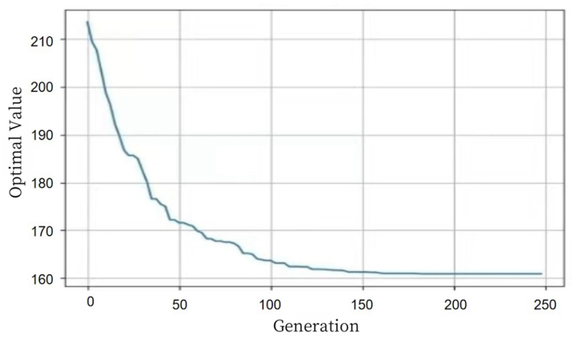
From an environmental sustainability perspective, the optimization effect of the PIVNS algorithm also manifests in ecological benefits. According to experimental data, the average travel distance of the PIVNS algorithm is 2020.85 km, which is 75.29 km less than that of the traditional VNS algorithm (2096.14 km). Referring to the industry-average carbon emission factor for light freight vehicles (0.18–0.22 kg/km), and using 0.20 kg/km for the calculation, a single delivery can reduce carbon emissions by approximately 15.06 kg. Assuming 300 operations per year, the annual emission reduction is about 4.52 tons, equivalent to a reduction of 9.04 tons of carbon dioxide (converted at a carbon–oxygen ratio of 1:2). This result confirms the direct role of shortening transportation mileage in reducing the environmental load of logistics systems, highlighting the value of the optimized scheme in green logistics practice. Based on the above analysis, the eighth run of the PIVNS algorithm in the example represents the optimal solution. Therefore, the eighth run is selected as the optimal solution for PIVNS, and the iteration trend of this experiment is shown in Figure 7.

As shown in Figure 7, the optimal value of the algorithm decreases significantly in the initial stages. The rate of decrease slows down around the 80th generation, and by the 100th generation, the output stabilizes, indicating convergence of the algorithm. Therefore, the algorithm exhibits strong optimization capability and converges quickly, finding satisfactory solutions in a short period of time. The optimized delivery routes consist of 10 routes, with the optimization results shown in

Table 6. Optimal schedule routes of PIACO algorithm.

Route	Load Rate (%)
C1-15-1-6-19-C1	85.13
C1-17-16-13-C1	87.49
C1-3-7-C2	86.48
C1-2-5-C2	85.98
C1-5-13-C1	88.71
C1-9-C2	85.16
C2-20-14-11-13-C2	86.48
C2-11-2-C2	84.78
C2-10-4-C2	87.23
C2-8-12-21-C2	90.31

below:

The Load Rate refers to the mean ratio of actual loaded volume to the maximum vehicle capacity across all delivery routes within each planning period. The values are calculated based on simulation outputs and represent the overall efficiency of vehicle utilization.

As shown in Table 6, in this case study, a subset of the part distribution routes involving two collection centers (C1 and C2) and 21 parts suppliers (1 to 21) is analyzed. Each supplier provides specific automotive parts, and the optimized parts pickup routes are as follows:

• Path 1: Start from C1, pass through suppliers 15, 1, 6, 19, and finally return to C1.
• Path 2: Start from C1, pass through suppliers 17, 16, 13, and finally return to C1.
• Path 3: Start from C1, visit suppliers 3, 7, and finally reach C2.
• Path 4: Start from C1, visit suppliers 2, 5, and finally reach C2.
• Path 5: Start from C1, pass through suppliers 5, 13, and finally return to C1.
• Path 6: Start from C1, visit supplier 9, and finally reach C2.
• Path 7: Start from C2, pass through suppliers 20, 14, 11, 13, and finally return to C2.
• Path 8: Start from C2, pass through suppliers 11, 2, and finally return to C2.
• Path 9: Start from C2, pass through suppliers 10, 4, and finally return to C2.
• Path 10: Start from C2, pass through suppliers 8, 12, 21, and finally return to C2.

Optimizing joint distribution routes enhances the cost-effectiveness and reduces transportation time for parts distribution. Specifically, for routes with multiple visits to certain suppliers or passing through two collection centers, such as Path 3 and Path 4, merging transportation tasks or re-planning the routes can effectively minimize redundancy and enhance efficiency. This not only lowers transportation costs but also speeds up delivery, thereby strengthening the competitiveness of the entire supply chain.

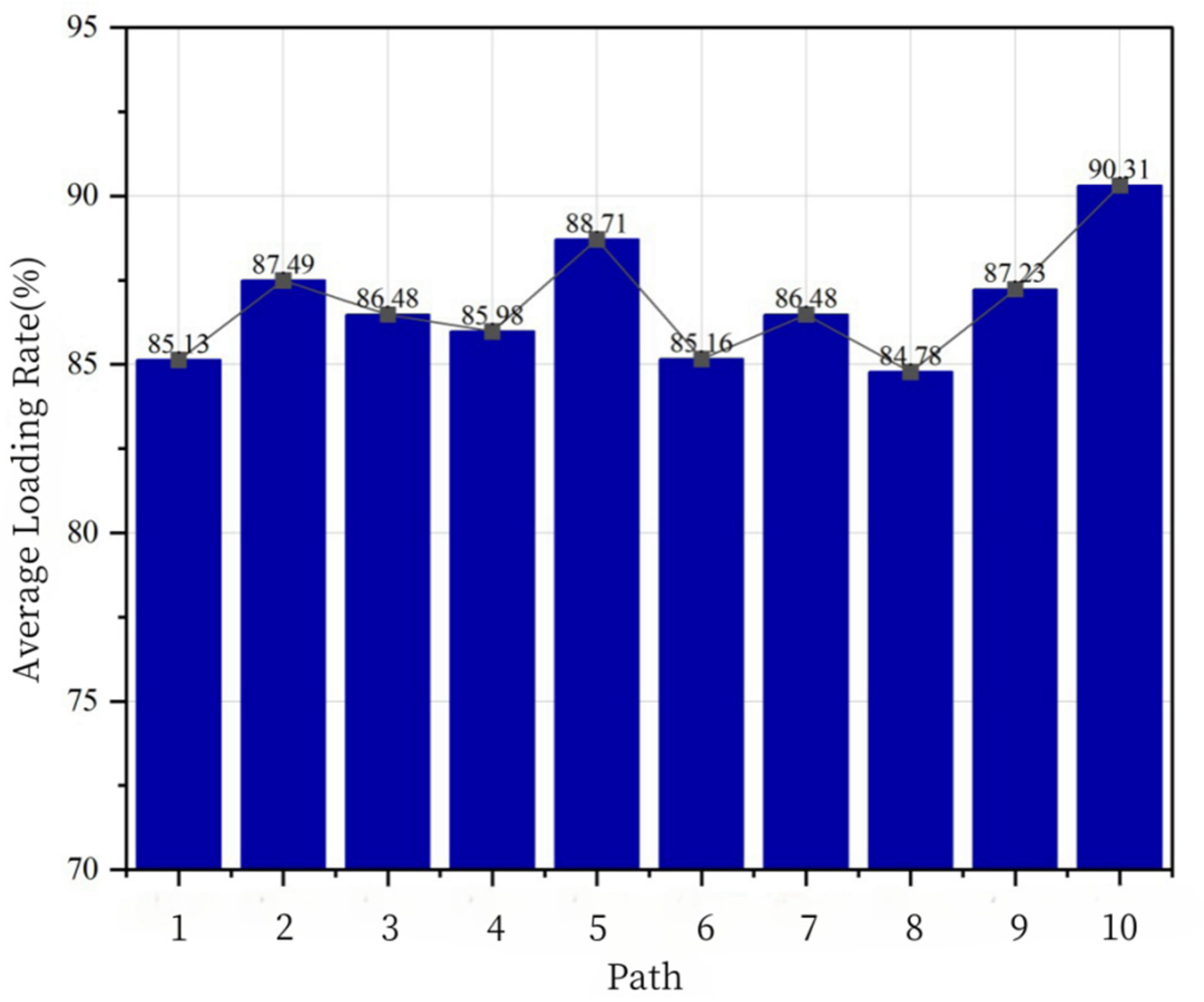
In this study, to assess the efficiency of parts distribution, the loading rates from suppliers to collection centers are carefully tested. Figure 8 shows the loading rates for each path in the eighth experiment, which display key indicators of transportation efficiency. As shown in Figure 8, the loading rates for Paths 1 to 10 are 81.79%, 81.19%, 79.54%, 76.82%, 81.30%, 77.16%, 80.65%, 78.90%, 78.94%, and 81.51%, respectively, with an average load rate of 79.78%. The highest loading rate reaches 81.79%, while the lowest is 76.82%. Notably, despite the loading rate in the eighth experiment not being the highest across all tests, it demonstrates substantial advantages in cost control and resource optimization. The results show that joint distribution route optimization, while maintaining a relatively high loading rate, yields the lowest distribution cost. This further highlights the practical application potential of the distribution strategy in achieving efficient resource utilization and reducing logistics costs.

5.2. Benchmark Experiment Comparison

To comprehensively assess the effectiveness and advantages of the PIVNS algorithm, this study compares the performance of PIVNS with traditional VNS and VNS with mutation operation (VNS-M). VNS-M is a metaheuristic algorithm incorporating mutation operations for solving complex combinatorial optimization problems. Consistent with previous experiments, each algorithm is tested 10 times, with both the optimal and average values recorded. The comparative performance results of PIVNS versus the baseline algorithms on the test case are presented in

Table 7. Comparison of PIACO with two ant algorithms.

Indicator		Algorithm
		ACO	ACO-WM	PIACO
Driving Distance (km)	Best	1913.6	1902.7	1886.1
	Average	2096.14	2051.78	2020.85
Running Time (s)	Best	110.25	105.5	102.2
	Average	115.16	113.9	112.25
Total Cost (CNY)	Best	12,238.72	11,998.39	11,864.67
	Average	12,687.84	12,545.78	12,497.99
Average Load Rate (%)	Best	85.61	86.14	90.31
	Average	80.45	84.81	86.775

, below.

As shown in Table 7, the VNS algorithm exhibits the highest average driving distance of 2096.14 km, indicating that the basic VNS algorithm has poor generalization ability for solving new problems. The VNS-M algorithm, which incorporates additional information, reduces the average transportation distance to 2051.78 km, while the PIVNS algorithm achieves the lowest average transportation distance of 2020.85 km, demonstrating its superior solution performance. This suggests that PIVNS, by incorporating parallelization and coarse-grained strategies, successfully expands the search space and effectively avoids local optima, resulting in a better driving path. Regarding running time, the VNS algorithm has an average transportation time of 115.16 s. This indicates that there is still room for improvement in terms of time efficiency. Following the introduction of additional information, VNS-M marginally reduces the transportation time to 113.9 s, though the improvement is minimal. In contrast, PIVNS has the lowest average transportation time of 112.25 s, demonstrating its advantage in path planning and transportation efficiency. Regarding total cost, the VNS algorithm has an average total cost of RMB 12,687.84, which may be attributed to its choice of longer paths and lower transportation efficiency. Upon the incorporation of additional information and strategies, VNS-M marginally reduces the total cost to RMB 12,545.78, yet the improvement is limited. On the other hand, the PIVNS algorithm achieves the lowest total cost, with an average of RMB 12,497.99, indicating significant advantages in cost control and resource utilization. For average load utilization, VNS has an average load utilization of 80.45%, which may suggest some inefficiency in optimizing load utilization. VNS-M shows an improvement, with a load utilization of 84.81%, highlighting the positive effect of the mutation operation in increasing load utilization. PIVNS possesses the highest average load utilization at 86.775%, indicating that PIVNS effectively improves resource utilization and reduces total delivery costs.

In conclusion, the PIVNS algorithm outperforms both VNS and VNS-M in terms of driving distance, transportation time, total cost, and resource utilization. By effectively integrating parallelization and coarse-grained strategies, PIVNS optimizes the delivery path and demonstrates substantial advantages in solving complex real-world logistics and distribution problems. Furthermore, VNS-M generally outperforms VNS, further substantiating the effectiveness of the mutation operation in enhancing algorithm performance.

6. Discussion

The optimization model for multi-manufacturer collaborative parts distribution proposed in this study, combined with the parallel improved variable neighborhood search (PIVNS) algorithm, demonstrates high computational efficiency and excellent performance in solving large-scale problems. Experimental results show that the proposed optimization method effectively reduces distribution costs and enhances overall supply chain efficiency, showcasing its feasibility and effectiveness in practical applications. Overall, while the proposed model and algorithm have demonstrated their effectiveness under the defined experimental conditions, their applicability is bounded by several structural assumptions. These include static demand scenarios, fixed fleet configurations, and pre-defined network parameters. Such conditions may not reflect the full complexity and dynamism of real-world logistics systems. As such, future extensions of this work could investigate the model’s adaptability under varying operational contexts, including stochastic demands, network disruptions, and heterogeneous fleet dynamics. Clearly delineating these boundaries also helps define the model’s scope of application, positioning it as a promising baseline for practical deployment under semi-controlled collaborative logistics environments. Future work may explore the integration of real-time traffic and weather data through predictive analytics, dynamic routing algorithms, or simulation-based optimization frameworks to enhance practical applicability.

The proposed PIVNS algorithm shows clear advantages in terms of solution quality and computational efficiency. From a practical standpoint, the cost savings achieved—averaging 8.7% compared to traditional single-depot routing—translate into fewer delivery vehicles needed and reduced operational cycles, which can significantly alleviate fleet pressure in real-world logistics systems. It should be emphasized that although the model takes total operational cost as the core optimization objective, the reduction in travel distance and the improvement in load rate (86.775% on average for PIVNS vs. 80.45% for traditional VNS) objectively reduce the carbon emission intensity per unit of goods. This ”cost reduction and emission reduction” synergistic effect stems from the inherent logic in logistics systems that “efficient resource utilization equals emission reduction”—reducing empty driving and improving load rates are themselves effective ways to reduce environmental impact. Therefore, the multi-manufacturer collaborative distribution model can achieve simultaneous improvements in economic efficiency and environmental sustainability without additional environmental protection investment. In particular, the ability to consolidate deliveries across multiple manufacturers enhances vehicle utilization and scheduling flexibility. Regarding real-world applicability, the model assumes accurate demand and route data, which is feasible in enterprises with established logistics information systems. However, its effectiveness may be influenced by data uncertainty or operational constraints in small-scale enterprises. Nevertheless, the approach remains compatible with current logistics management systems and can be adapted to dynamic dispatching scenarios with further extensions. In terms of sustainability, the reduction in total distance traveled and better load balancing imply lower fuel consumption and emissions. The results suggest that multi-manufacturer collaboration, supported by efficient algorithmic scheduling, can contribute to greener logistics by decreasing resource waste and redundant trips. Compared with previous algorithms such as standard VNS and genetic algorithms, PIVNS demonstrates superior convergence speed and robustness across diverse instance scales. Unlike most prior studies that optimize routing for single enterprises, this model accommodates shared resources and dynamic depot selection, making it more suitable for integrated supply chains and joint distribution networks. However, the limitations of this study must also be acknowledged. Specifically, the model assumes constant vehicle speeds and road conditions, neglecting dynamic factors such as traffic, weather changes, and road maintenance that may impact the actual transportation process. Future studies could consider incorporating these dynamic factors to improve the model’s adaptability and accuracy.

Moreover, while this study offers an effective solution for collaborative distribution among multiple manufacturers, it assumes a fixed fleet size and vehicle type, which may not fully capture real-world complexities. Fleet size and vehicle types can change according to demand and resource variations. In practical scenarios, fleet size and vehicle type often vary with time, region, and operational objectives. These variations can be influenced by factors such as seasonal demand, contractual constraints with logistics providers, and differences in vehicle operating costs. While our model assumes a fixed configuration for tractability and benchmarking purposes, this simplification may limit its applicability in highly dynamic environments. Future research could incorporate adaptive fleet modeling techniques that allow for flexible vehicle assignment based on operational data, such as demand fluctuations or fuel efficiency considerations. Therefore, future research could explore strategies for dynamically adjusting fleet size and vehicle types to further enhance distribution efficiency. Additionally, the current model and algorithm are designed for known distribution networks. Future work should address maintaining computational efficiency and solution quality in more complex and dynamic network environments.

This study contributes by filling the research gap in optimizing collaborative distribution paths among multiple manufacturers. The existing literature primarily examines distribution path optimization for single factories, often overlooking the collaborative operations between multiple factories. By proposing an optimization model that adapts to multi-factory collaboration, this study provides new insights for logistics optimization in the automotive manufacturing industry and offers valuable references for research and applications in similar fields. Future research may incorporate emerging technologies such as the IoT, big data, and blockchain to advance the intelligence, real-time capability, and transparency of distribution path optimization, thereby fostering the intelligent and sustainable development of supply chain management.

More specifically, the proposed strategy contributes to supply chain sustainability by reducing redundant routes and fuel consumption, enhancing vehicle utilization, and facilitating coordinated delivery practices that align with the principles of responsible and energy-efficient logistics.

7. Conclusions

This paper initially highlights the importance of the automotive parts distribution problem in multi-manufacturer collaboration within the modern automotive industry’s supply chain. It details the characteristics of the multi-manufacturer collaborative distribution problem and establishes a mathematical model that comprehensively considers geographical distribution, demand volume, and production pace. The goal is to optimize the distribution routes to reduce transportation costs and improve overall supply chain efficiency. To address this complex problem, this paper proposes an improved Variable Neighborhood Search (VNS) algorithm with a virtual distribution center (PIVNS), which effectively simplifies the complexity of the problem and enhances solution efficiency.

The results collectively demonstrate that the proposed PIVNS algorithm outperforms the traditional VNS algorithm and the VNS algorithm with mutation operation (VNS-M) across key performance indicators. Specifically, in terms of driving distance, the average driving distance of the PIVNS algorithm is 2020.85 km, which is 3.51% and 1.52% lower than VNS and VNS-M, respectively. In terms of runtime, PIVNS achieves an average runtime of 112.25 s, representing improvements of 2.90% and 1.47% compared to VNS and VNS-M, respectively. Regarding total cost, the average total cost of PIVNS is RMB 12,497.99, which is 1.35% and 0.36% lower than that of VNS and VNS-M, respectively. Additionally, PIVNS demonstrates the highest average load utilization at 86.775%, exceeding VNS and VNS-M by 9.68% and 2.87%, respectively. These results indicate the outstanding performance of the PIVNS algorithm across multiple key metrics, including driving distance, transportation time, total cost, and load utilization, further proving its effectiveness and practicality in solving the multi-manufacturer collaborative distribution problem. By reducing driving paths and improving load utilization, the PIVNS algorithm both optimizes resource allocation and significantly reduces logistics costs, providing an efficient and cost-effective distribution strategy for supply chain management. Meanwhile, the optimized scheme achieves an annual emission reduction of approximately 4.5 tons by shortening transportation distance and improving vehicle utilization, providing a quantifiable, practical path for the green transformation of automotive parts supply chains.