Article

Research on a Short-Term Electric Load Forecasting Model Based on Improved BWO-Optimized Dilated BiGRU

Faculty of Electrical and Control Engineering, Liaoning Technical University, Huludao 125000, China
*
Author to whom correspondence should be addressed.
Sustainability 2025, 17(21), 9746; https://doi.org/10.3390/su17219746
Submission received: 17 June 2025 / Revised: 2 October 2025 / Accepted: 27 October 2025 / Published: 31 October 2025

Abstract

In the context of global efforts toward energy conservation and emission reduction, accurate short-term electric load forecasting plays a crucial role in improving energy efficiency, enabling low-carbon dispatching, and supporting sustainable power system operations. To address the growing demand for accuracy and stability in this domain, this paper proposes a novel prediction model tailored for power systems. The proposed method combines Spearman correlation analysis with modal decomposition techniques to compress redundant features while preserving key information, resulting in more informative and cleaner input representations. In terms of model architecture, this study integrates Bidirectional Gated Recurrent Units (BiGRUs) with dilated convolution. This design improves the model’s capacity to capture long-range dependencies and complex relationships. For parameter optimization, an Improved Beluga Whale Optimization (IBWO) algorithm is introduced, incorporating dynamic population initialization, adaptive Lévy flight mechanisms, and refined convergence procedures to enhance search efficiency and robustness. Experiments on real-world datasets demonstrate that the proposed model achieves excellent forecasting performance (RMSE = 26.1706, MAE = 18.5462, R2 = 0.9812), combining high predictive accuracy with strong generalization. These advancements contribute to more efficient energy scheduling and reduced environmental impact, making the model well-suited for intelligent and sustainable load forecasting applications in environmentally conscious power systems.

1. Introduction

In modern society, electricity serves as a fundamental supporting energy source, widely used in critical sectors such as industry, transportation, and healthcare. Power load forecasting constructs models to accurately predict electricity demand, providing a scientific basis for power system planning and operation. It not only optimizes system performance and reduces operational costs but also plays a crucial role in energy conservation, emissions reduction, and sustainable socio-economic development. By leveraging statistical analysis, time series modeling, and neural network approaches, power load forecasting extracts patterns from historical consumption data to construct predictive models that enable accurate forecasting of future loads. These forecasts serve as critical references for system planning and scheduling, helping electricity management authorities to arrange generation plans rationally and mitigate the risks of power shortages or surpluses.
As a core task for maintaining power supply–demand balance and improving system operational efficiency, short-term power load forecasting has consistently remained at the forefront of power data research. With the continuous advancement of mathematical theory and the exponential growth in computational power, forecasting technologies in this field have undergone a profound evolution—from traditional to intelligent methods, and from linear to nonlinear modeling. Broadly, they can be categorized into three major technical systems: statistical methods, machine learning methods, and deep learning methods [1].
In the early stages of electricity load forecasting development, statistical methods, due to their solid theoretical foundation and high computational efficiency, became the mainstream technology of the time. These methods primarily use time as the main variable, constructing mathematical models based on time series analysis to forecast electricity load. However, traditional statistical models often rely on linear assumptions [2], whereas nonlinear and non-stationary characteristics are widespread in power systems [3]. For example, the diversity of user consumption behaviors and the integration of some distributed energy sources on the user side can both affect the load data’s variation patterns, thus reducing the model’s prediction accuracy and generalization ability [4]. In recent years, as the scale of power systems has expanded and renewable energy has been widely integrated on both the generation and grid sides, the overall operating mechanisms of the system have become more complex, placing higher demands on load forecasting models. As a result, traditional statistical methods are increasingly unable to meet the growing accuracy requirements.
In recent years, the rapid advancement of hardware technologies has laid a solid foundation for the rise of machine learning and deep learning techniques, ushering in a new technological paradigm for power load forecasting. As a vital branch of artificial intelligence, machine learning—through classic algorithms such as Random Forest (RF) [5] and Support Vector Machine (SVM) [6]—can perform preliminary feature selection and pattern recognition on power data, thereby enhancing model capability in handling complex datasets. Grzegorz Dudek was among the first to apply RF to short-term power load forecasting, establishing a foundation for RF-based research in this field [7]. Subsequently, Bianca Magalhães and others further explored RF’s potential by constructing regression trees using a combination of bagging and random subspace techniques, aiming to improve forecasting accuracy and model stability [8]. Guo-Feng Fan proposed a Support Vector Regression (SVR) model that integrates Differential Empirical Mode Decomposition (DEMD) and Auto Regression (AR). This model decouples high- and low-frequency components in the load data, effectively uncovering deep latent features in the sequence and enhancing forecasting performance [9]. Based on traditional models, ensemble methods such as Gradient Boosting Decision Trees (GBDTs) and their efficient variant XGBoost have increasingly been adopted in power load forecasting. By combining weak learners to enhance overall performance, these models exhibit strong nonlinear modeling capabilities, particularly suited for multivariate and high-dimensional load data. Beibei Chen applied clustering techniques to the load data and then used GBDT for forecasting, comparing its results with those of RF and SVR. The findings demonstrated that GBDT, as an ensemble method, achieves higher accuracy and stability when modeling complex load patterns [10]. Raza Abid Abbasi utilized XGBoost for both feature selection and load forecasting, providing strong empirical support for its use in short-term forecasting tasks [11]. However, as the complexity and diversity of power data continue to increase, the limitations of machine learning methods have become increasingly apparent [12]. For instance, traditional models often struggle with capturing long-range temporal dependencies or adapting to non-stationary patterns caused by renewable integration and user behavior variability [13].
Deep learning has profoundly transformed the field of power load forecasting, breaking through the limitations of traditional methods. Deep learning models represented by Recurrent Neural Networks (RNNs) [14] and their variants—Long Short-Term Memory (LSTM) networks [15] and Gated Recurrent Units (GRUs)—have significantly improved the accuracy and stability of load forecasts. These models possess powerful automatic feature extraction capabilities, reducing the reliance on manual feature engineering and enabling the discovery of deep patterns in large-scale power data. Building upon this, some researchers have proposed bidirectional models such as Bidirectional LSTM (BiLSTM) [16] and BiGRU, which capture both forward and backward flows of temporal information to enhance the perception of sequential features in load data. Deep learning models, by constructing complex and adaptive architectures, effectively capture hidden, dynamic patterns within power load data. Bharat Bohara integrated Convolutional Neural Networks (CNNs) with BiLSTM to expand the receptive field of BiLSTM, achieving improved forecasting accuracy [17]. Yuting Lu proposed a hybrid structure combining CNN and BiGRU, which outperformed conventional benchmark models across multiple evaluation metrics, validating its effectiveness in load forecasting [18]. These studies demonstrate that deep learning models, when handling large-scale and high-dimensional power data, outperform traditional methods in managing nonlinear characteristics and deliver significantly improved forecasting accuracy.
Despite achieving high accuracy, deep learning models still face challenges such as interference from redundant features and insufficient utilization of frequency-domain information. A large number of weakly correlated features may hinder model training, and critical information in different frequency bands is often overlooked when processed uniformly. To address these issues, this paper proposes a well-designed novel forecasting model. First, a feature engineering method based on Spearman correlation analysis is used to assess correlations within the original dataset, categorizing features into high-value and low-value groups. For high-value features, Variational Mode Decomposition (VMD) is used to extract and retain high-frequency components. Meanwhile, the low-frequency components of high-value features are fused with those extracted from low-value features via Complete Ensemble Empirical Mode Decomposition with Adaptive Noise (CEEMDAN) to preserve key elements from low-value features that significantly influence the load.
The proposed Improved Beluga Whale Optimization algorithm is then used for model hyperparameter tuning, addressing the shortcomings of manual tuning. For the forecasting model itself, the core innovation lies in the Dilated BiGRU architecture, which embeds dilated convolution into the gating mechanism of the Bidirectional GRU. This design enables unified modeling of short- and long-term dependencies, effectively addressing the limitations of traditional GRUs, such as restricted local perception due to fully connected gating and inefficiencies in modeling long-period dependencies. It also overcomes deficiencies in dynamic temporal modeling and bidirectional information fusion. By explicitly expanding the receptive field through configurable dilation rates, the gating computation can directly connect across key time points. In addition, the shared local weights of convolution enhance sensitivity to short-term fluctuations. In the context of power load forecasting, the bidirectional dilated gating mechanism captures complex dependencies both from past to future and future to past, balancing computational efficiency with forecasting accuracy, and significantly boosting the model’s ability to jointly model multi-scale temporal patterns. Experimental results show that the proposed model performs excellently in short-term forecasting tasks, achieving RMSE, R2, and MAE scores of 26.1706, 0.9812, and 18.5462, respectively.

2. Materials and Methods

2.1. Feature Engineering

Proper data processing has always been one of the most critical components in time series forecasting tasks, as data quality is a key factor that determines the accuracy of prediction results. In other words, constructing appropriate feature engineering is not only the first step but also a crucial step in achieving high-accuracy power load forecasting.
Derni Ageng et al. applied Savitzky–Golay filtering to raw data and input the smoothed data into an LSTM model for short-term load forecasting, verifying the significant role of data preprocessing in enhancing model performance [19]. In comparison, Qiu Sun et al. introduced Variational Mode Decomposition before filtering and fed the VMD- and Savitzky–Golay-processed data into an LSTM model. Experimental results showed that this combined method improved the model’s sensitivity to load fluctuation features [20]. Haixiang Zang et al. further decomposed datasets containing meteorological features using VMD and combined the results with an LSTM model enhanced by a self-attention mechanism, which significantly improved forecasting accuracy under multi-feature conditions [21]. Ghulam Hafeez et al. employed Grey Correlation Analysis (GCA) and Kernel Principal Component Analysis (KPCA) to eliminate redundant features and reduce dimensionality, and then input the processed features into an SVM optimized by a modified Enhanced Differential Evolution (mEDE) algorithm, which led to improved predictive performance [22].
The above studies indicate that current feature engineering methods are mostly based on single signal decomposition techniques or fail to deeply mine the latent information in data following correlation analysis. Although such approaches can reduce workload and computational costs to some extent, the quality of the features obtained is often suboptimal. To improve data quality, this paper designs a novel feature engineering framework. By integrating Spearman correlation analysis, VMD [23], and CEEMDAN [24], the proposed method separates high- and low-frequency components from the feature sequences while preserving the original dataset’s richness in feature information. The process flow is illustrated in Figure 1.
Figure 1 illustrates the feature engineering process proposed in this paper, which combines Spearman correlation analysis with modal decomposition strategies. This approach enhances feature effectiveness and structural expressiveness while preserving the diversity of the original features. Specifically, Spearman correlation is first applied to quantify and screen the relevance between each feature and the forecasting target. For features with low correlation, the CEEMDAN method is employed to retain only their low-frequency components, thereby mitigating noise interference. For features with high correlation, the VMD method is applied to perform multi-modal decomposition, extracting both high- and low-frequency components. Ultimately, all preserved low-frequency components are integrated to construct a multi-scale, low-redundancy feature set. This processing framework jointly leverages correlation-based screening and frequency-domain modeling, simultaneously compressing redundant information and enhancing the representation of key features, thus enabling the model to better capture variations and patterns in time series data.
This study uses the Panama short-term electricity load forecasting dataset from the Kaggle platform (https://www.kaggle.com/datasets/ernestojaguilar/shortterm-electricity-load-forecasting-panama (accessed on 15 May 2025.)) as experimental data. The dataset was organized by the Panama grid operator based on daily dispatch reports, reflecting the overall electricity load of the city and covering multiple user categories, including residential, commercial, and industrial users, making it highly representative. The data is recorded at an hourly frequency, spanning from 3 January 2015, to 27 June 2020. The electricity load features include 48,048 samples. In addition, the dataset provides environmental variables such as temperature, humidity, wind speed, and time information, all of which are closely related to load variations. The total number of samples for all features is 768,768, forming a typical multivariate time series data structure suitable for electricity load forecasting tasks.
This study uses data from 1 January 2019 to 1 June 2020 within the dataset as the modeling and experimental sample. The dataset includes a total of 9 feature variables, all of which were included in the modeling process with electricity load values as the prediction target. Each feature contains 12,431 records, resulting in a total of 111,879 data points. Detailed feature names and variable descriptions can be found in Table 1.
To validate the performance of the proposed forecasting model, the dataset is divided into a training set and a testing set in a 70% to 30% ratio. The training set contains 78,316 data points and is used for model training, while the testing set comprises 33,563 data points and is used to evaluate the model’s predictive capability on unseen data. This large-scale dataset provides sufficient informational support for model training. However, it also incurs substantial computational costs, particularly during the training phase, placing higher demands on hardware performance and training time. Furthermore, not all features are highly correlated with the load; the inclusion of low-correlation features may reduce forecasting accuracy. Therefore, this paper employs the Spearman correlation algorithm to calculate the correlation between each feature and the target variable. The formula is defined as follows:
ρ = i = 1 N R x i R ¯ x R y i R ¯ y i = 1 N R x i R ¯ x 2 i = 1 N R y i R ¯ y
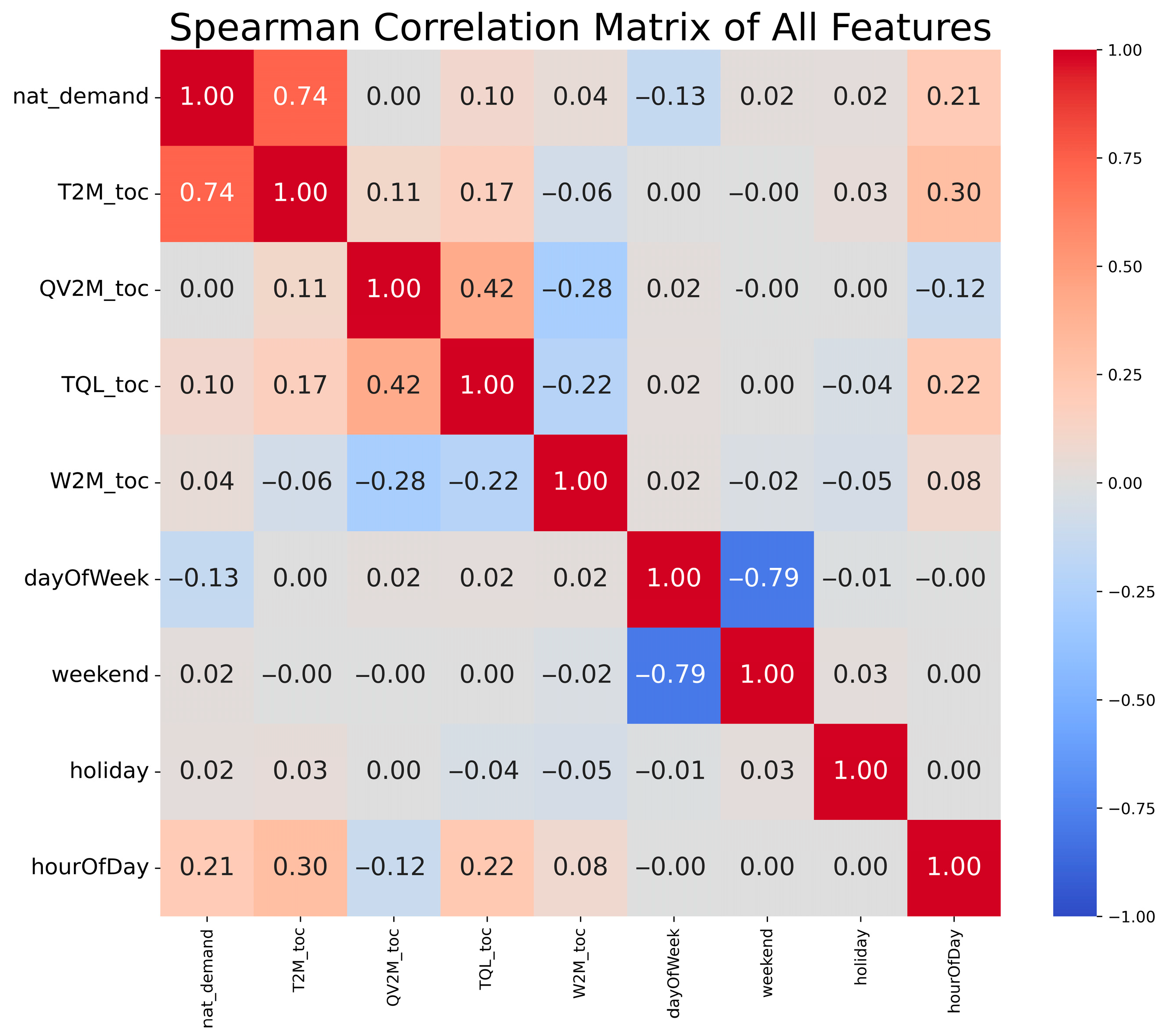
where ρ denotes the Spearman rank correlation coefficient. R x i and R y i represent the ranks of the corresponding values x i and y i for any two selected features, while R ¯ x and R ¯ y denote the mean ranks. The results obtained from the Spearman correlation coefficients are visualized in the form of a heatmap, as shown in Figure 2.
Figure 2 presents the results of feature correlation analysis on the original dataset based on Spearman correlation. The color scale ranges from dark blue to dark red, corresponding to correlation coefficients from −1 to 1. The closer the color is to red, the stronger the positive correlation; the closer to blue, the stronger the negative correlation; and lighter colors indicate weaker or near-zero correlations. As shown in the figure, the electricity load (nat_demand) has the highest correlation with temperature (T2M_toc), with a Spearman coefficient of 0.74, indicating a significant positive relationship. In contrast, the correlations between load and other features such as specific humidity (QV2M_toc) and wind speed (W2M_toc) are much weaker and close to zero, suggesting that their impact on load variation is limited.
For features with low correlation, this study does not adopt the common approach of direct elimination. Instead, the CEEMDAN algorithm is applied to decompose such features, removing high-frequency ineffective components while retaining the low-frequency parts. This allows the prediction model to learn potential long-term trend information embedded in the original sequences and uncover hidden patterns that may serve as valuable supplementary signals for load forecasting. This strategy improves the utilization of low-correlation features and prevents potentially useful information from being discarded during preprocessing.
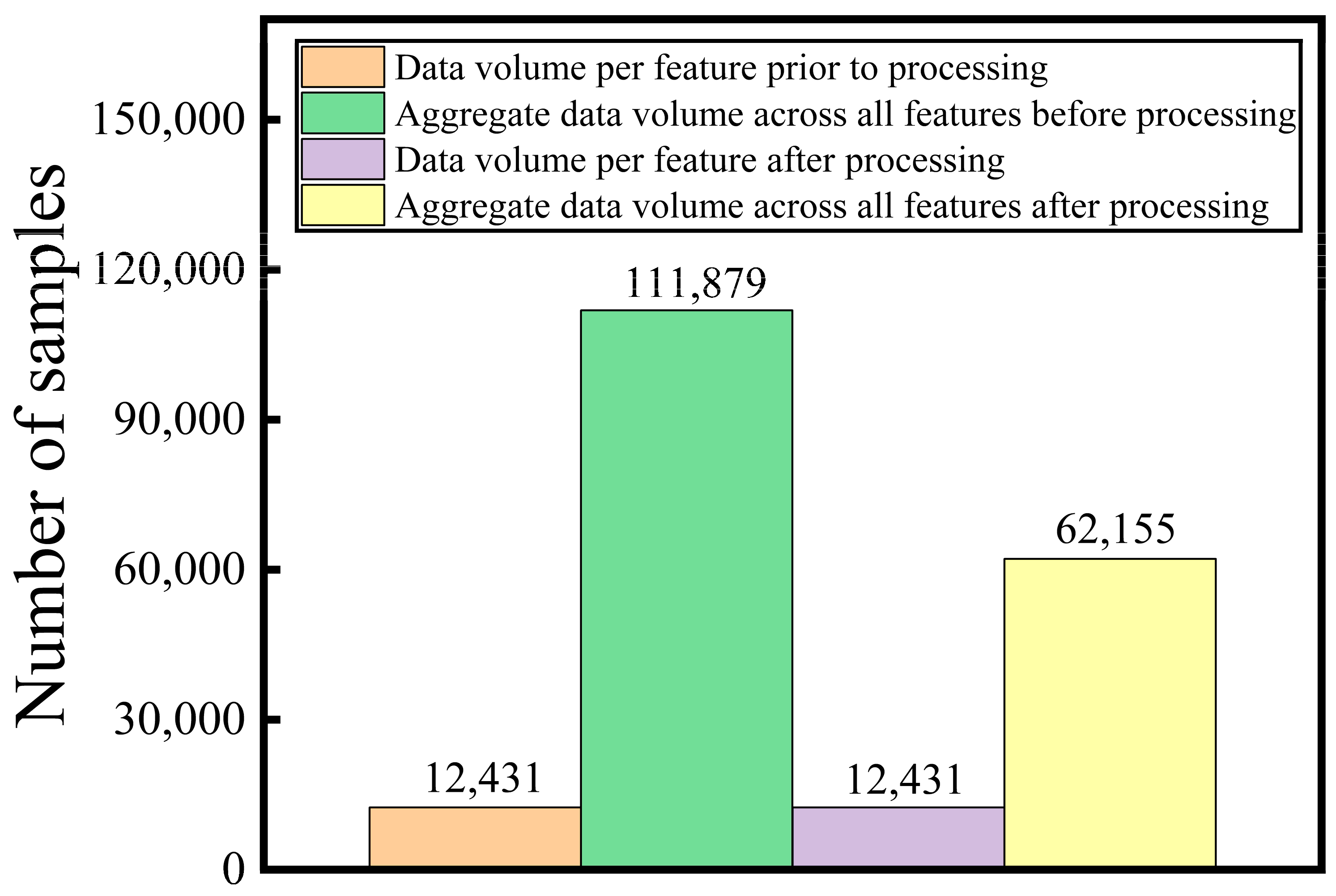
For features highly correlated with the load, such as T2M_toc and hourOfDay, the VMD method is employed to decompose each feature curve into high-frequency and low-frequency components, thereby extracting multi-scale feature information. The load variable itself (nat_demand) is also decomposed using VMD to capture its hierarchical temporal characteristics and enhance the model’s ability to fit load trends. Subsequently, the low-frequency components of all features obtained through CEEMDAN and VMD are merged into a unified long-term trend curve to improve the model’s performance in capturing long-term variations. Meanwhile, the high-frequency components of strongly correlated features are fully retained to preserve sensitivity to short-term fluctuations. Figure 3 shows a comparison of data volume before and after feature processing, and Table 2 lists the final input feature composition and sample counts of the dataset used in the model.
As shown in Figure 3 and Table 2, the dataset was reduced by 49,724 time steps after feature engineering, effectively compressing its overall scale. While preserving critical information, the removal of redundant and noisy data helps reduce the computational burden during model training and improves both the stability and efficiency of the training process. The resulting lightweight dataset significantly lowers computational overhead, making the model more suitable for deployment in resource-constrained or real-time application scenarios.
Figure 4 displays the Spearman correlation results between the processed features and the load values. The processed features include high-frequency components extracted via VMD and low-frequency components derived from the fusion of CEEMDAN and VMD outputs. Most of the processed features exhibit strong correlations with the load values, indicating their high effectiveness in characterizing load variations. Specifically, the high-frequency component of temperature shows a Spearman correlation coefficient as high as 0.74 with the load, reflecting a strong synchronization between temperature fluctuations and load dynamics. The high-frequency component of the load itself has a correlation of 0.40 with the original load, suggesting that the VMD captures local fluctuations while still preserving part of the global trend. Additionally, the fused low-frequency component (denoted as “low”) yields a correlation coefficient of 0.46 with the load, outperforming the original undecomposed features, thus validating the effectiveness of the feature fusion process. Overall, these time–frequency decomposed and fused features accurately characterize the patterns of load variation across multiple temporal scales, providing a solid foundation for subsequent model construction and prediction.
Figure 5 presents the performance differences among three representative RNN-based prediction models, namely GRU, BiLSTM, and BiGRU, under three different feature processing schemes. The first scheme retains all high- and low-frequency components obtained from signal decomposition as input data. The second scheme uses the original data directly. The third scheme applies the feature processing method proposed in this study.
From Figure 5 and Table 3, it is evident that the first scheme, although significantly increasing the data dimensionality, does not outperform the raw input in terms of prediction accuracy. In fact, some metrics show a slight decline. For example, the RMSE of the GRU model with all components retained is 68.5934, which is higher than the 65.8601 with the raw input. BiLSTM and BiGRU exhibit similar trends, with RMSE values of 65.7128 and 64.2005, both higher than the original input values of 65.6279 and 62.5517, respectively. This indicates that blindly including all frequency components may lead to increased redundant or noisy information, thereby affecting the model’s performance.
In contrast, the feature selection and decomposition strategy proposed in this study is theoretically well-grounded and has demonstrated strong effectiveness in engineering practice. We first evaluate the correlation between each feature and the target load, and classify them into strongly correlated and weakly correlated groups accordingly. During feature processing, we do not treat all high-frequency components as noise indiscriminately; instead, we apply a differentiated strategy based on the level of correlation.
For strongly correlated features, we retain all frequency components, including the high-frequency parts. These high-frequency fluctuations capture short-term variations such as holidays, extreme weather events, and sudden load changes, all of which have a significant impact on load forecasting accuracy. In contrast, the high-frequency components of weakly correlated features interfere with model training, while their low-frequency components capture long-term trends and provide clear, structured, and informative input to the model. Therefore, we retain only the low-frequency components of weakly correlated features, which fundamentally enhances the quality of input data and improves model stability.
The experimental results demonstrate that this strategy significantly improved model performance. Using the proposed processing method, the RMSE of GRU decreased to 61.3893, BiLSTM decreased to 60.0619, and BiGRU further decreased to 52.3161, with accuracy outperforming the other two schemes. At the same time, the R2 metric significantly improved, with BiGRU rising from 0.8904 with the raw input to 0.9132, and the MAE decreased from 48.3497 to 39.8785. This further validates the rationality and wide applicability of the feature engineering strategy proposed in this paper in reducing redundancy and enhancing modeling efficiency.
Furthermore, this method reflects a core design principle: although all relevant information theoretically exists within the original dataset, in real-world scenarios characterized by high dimensionality and noise, relying solely on the model to automatically learn all effective patterns is inefficient and highly susceptible to interference, ultimately degrading performance. Large-scale models capable of such tasks demand substantial data, computational resources, and deployment infrastructure, making them impractical for many real-world load forecasting applications. The proposed feature processing strategy not only improves the quality of input features but also explicitly extracts structural trend information, thereby enhancing the model’s perception of long-term patterns. This strategy is deployable in engineering practice and is supported by both strong adaptability and solid theoretical foundations.

2.2. Beluga Whale Optimization

Beluga Whale Optimization (BWO) [25] addresses optimization problems by simulating the natural behavior of beluga whales. The algorithm consists of four main stages: population initialization, exploration phase, exploitation phase, and whale fall phase. Due to its excellent convergence speed and accuracy, BWO has been widely applied in various engineering optimization problems.

2.2.1. Population Initialization

BWO is a population-based algorithm that treats beluga whales as search agents, where each whale represents a candidate solution that is iteratively updated during the optimization process. The positions of the search agents are modeled in matrix form as
X = x 1 , 1 x 1 , 2 x 1 , d x 2 , 1 x 2 , 2 x 2 , d x n , 1 x n , 2 x n , d
where n is the population size of beluga whales, and d is the dimensionality of the design variables. The corresponding fitness values F x for all whales are stored as follows:
F x = f ( x 1 , 1 , x 1 , 2 , , x 1 , d ) f ( x 2 , 1 , x 2 , 2 , , x 2 , d ) f ( x n , 1 , x n , 2 , , x n , d )
The transition of the BWO algorithm from the exploration phase to the exploitation phase is determined by the balance factor B f , which is defined by the following formula:
B f = B 0 ( 1 T / 2 T max )
where T is the current number of iterations, T max is the maximum number of iterations, and B 0 is a random value that changes within the range (0, 1) at each iteration. When the balance factor B f > 0.5 , the algorithm remains in the exploration phase; when B f < 0.5 , it switches to the exploitation phase.

2.2.2. Exploration Phase

Inspired by the behavior of beluga whales acting in pairs, the algorithm defines the position update mechanism of the search agents using the following formulation:
X i . j T + 1 = X i . P j T + ( X r . P 1 T X i . P j T ) ( 1 + r 1 ) sin ( 2 π r 2 ) , j = e v e n X i . j T + 1 = X i . P j T + ( X r . P 1 T X i . P j T ) ( 1 + r 1 ) cos ( 2 π r 2 ) , j = o d d
where T is the current iteration number, X i . j T + 1 represents the new position of the i-th beluga whale in the j-th dimension. X i . P j T denotes the position of the i-th whale in the P j -th dimension, while X i . P j T and X r . P 1 T represent the current positions of the i-th and r -th whales, respectively. Here, r is a randomly selected integer within the range [1,N], where N is the population size. r 1 and r 2 are random numbers drawn from the interval (0, 1).

2.2.3. Exploitation Phase

During the exploitation phase, the BWO algorithm incorporates the Lévy flight strategy to enhance convergence behavior. The mathematical formulation for prey search using Lévy flight is expressed as follows:
X i T + 1 = r 3 X b e s t T r 4 X i T + C 1 L F ( X r . P j T X i T )
where T is the current iteration number, X i T and X r . P j T denote the current positions of the i-th beluga whale and a randomly selected whale, respectively. X i T + 1 is the new position of the i-th whale, and X b e s t T is the best position found among all whales. r 3 and r 4 are random numbers in the range (0, 1), and C 1 = 2 r 4 ( 1 T / T max ) is a random jump strength factor that quantifies the intensity of the Lévy flight. L F represents the Lévy flight function, which is calculated as follows:
L F = 0.05 × u × σ v 1 / β
σ = Γ ( 1 + β ) × sin ( π β / 2 ) Γ ( ( 1 + β ) / 2 ) × β × 2 ( β 1 ) / 2 1 / β
Here, u and v are random variables drawn from a normal distribution, and β is a predefined constant set to 1.5.

2.2.4. Whale Fall Phase

The life behavior of beluga whales suggests that they either migrate or experience whale fall, sinking into the deep sea. To maintain a constant population size, BWO formulates a position update equation that incorporates the current position of the whale and a descent step associated with whale fall:
X i T + 1 = r 5 X i T r 6 X i T + r 7 X s t e p
In this equation, r 5 , r 6 , and r 7 are random numbers in the range (0, 1), and X s t e p is the whale fall step size, which is defined as follows:
X s t e p = ( u b l b ) exp ( C 2 T / T max )
Here, C 2 is the step factor which is related to the probability of whale fall and population size ( C 2 = 2 W f × n ), u b and l b are the upper and lower boundary of variables, respectively. In this model, the probability of whale fall ( W f ) is calculated as a linear function:
W f = 0.1 0.05 T / T max

2.3. Improved Beluga Whale Optimization

Despite demonstrating certain advantages in various optimization tasks, BWO still exhibits limitations in complex search spaces. First, the algorithm uses completely random initialization for the population, which may lead to uneven distribution of search points in high-dimensional spaces, thereby restricting early-stage global exploration capability. Second, the use of fixed parameters in the Lévy flight mechanism results in a lack of phase-specific adjustment in the search behavior, which may cause premature convergence in the early stage and insufficient refinement during the exploitation phase. In addition, the standard BWO overly relies on the current best solution when updating individuals, lacking an effective mechanism for maintaining population diversity.
To address these issues, this paper proposes three improvement strategies: (1) introducing a dynamic tanh-Sobol sequence to enhance the quality of the initial population; (2) designing a dynamic Lévy flight mechanism to reinforce both exploration and exploitation capabilities; and (3) improving the structure of the whale fall step to increase the algorithm’s ability to escape from local optima in the later stages, thereby enhancing the robustness and global search capability of the model.

2.3.1. Tanh-Sobol Population Initialization

To address the problem of high randomness and uneven sample distribution in the initial population of the BWO algorithm, this paper introduces a dynamic tanh-Sobol sequence as the initialization strategy. This approach combines the low-discrepancy property of the Sobol sequence with the Matoušek–Affine–Owen scrambling technique to enhance uniformity in high-dimensional spaces. At the same time, a hyperbolic tangent (tanh) function is used to nonlinearly compress and regulate the amplitude of perturbations, allowing adaptive control over sample distribution density during initialization. This enhances boundary coverage and space-filling capability, thereby providing a higher-quality starting point for the subsequent optimization process. The specific procedure is as follows:
  • Define the population dimension as d , the upper bound of the search space as u b , the lower bound as l b , and let B o u n d a r y represent the search domain.
  • First, call the S o b o l s e t function to generate a Sobol sequence and assign it to the variable X , where X is defined as
    X = S o b o l ( d )
  • To retain the spatial uniformity and low discrepancy properties of the Sobol sequence while introducing greater randomness, this paper applies the Matoušek–Affine–Owen scrambling method to the original Sobol sequence. The corresponding formula is shown below. This method ensures that the generated population exhibits different point distribution characteristics in each run, making it particularly suitable for optimization algorithms that require multiple independent initializations.
    X = S c r a m b l e ( X , M a t o u s e k A f f i n e O w e n )
  • To address the issue that traditional Sobol sequence initialization methods exhibit excessive regularity and insufficient randomness, this paper proposes an improved method based on nonlinear function perturbation. The formula is defined as follows:
    x = x + δ × t a n h ( r a n d ( N , d ) × n )
Here, x represents the value generated by the original Sobol sequence, and x is the perturbed population point. δ is the perturbation factor used to control the amplitude of the perturbation, which is set to 0.01 in this study. The function r a n d N , d generates a random number matrix within the interval [0, 1]. n is the individual index ranging from 1 to N. tanh ( · ) is the hyperbolic tangent function, and its formulation is as follows:
tanh ( x ) = e x e x e x + e x
This perturbation enhances the uniformity of the generated population. Moreover, since the value of the tanh ( x ) function lies within the interval (−1, 1), it effectively constrains the perturbation magnitude.
5.
To ensure that the perturbed population points remain within the interval [0, 1] after applying the disturbance, boundary correction is applied, as defined by the following formula:
x = m a x ( m i n ( x , 1 ) , 0 )
Figure 6 and Figure 7 illustrate the sample distributions generated by random initialization and tanh-Sobol initialization in two-dimensional and three-dimensional spaces, respectively. Comparing the two figures, it is evident that the population generated by the random method is unevenly distributed, with densely clustered and empty regions, making it difficult to fully cover the search space. In contrast, the tanh-Sobol initialization yields a more uniform and structured distribution, demonstrating especially good boundary coverage. In Figure 6 and Figure 7, the colors of the generated population points have no specific meaning and are used solely for visual enhancement.
The comparison of population distribution results between the two initialization methods shows that the proposed tanh-Sobol initialization strategy effectively improves population quality. It provides the optimization algorithm with a more representative and diverse set of initial solutions, thereby enhancing global search performance.

2.3.2. Dynamic Lévy Flight Mechanism

In the original BWO, the stability index parameter α used for step size control is fixed, which often results in poor capability to escape local optima and weakens the overall search ability of the algorithm, potentially preventing convergence to the global optimum. To address this issue, this paper introduces a dynamic Lévy flight mechanism and proposes a novel adaptive regulation scheme for the parameter α , defined by the following formula:
α ( T ) = 1.3 + 1.7 1.3 1 e 5 T / T max
where T represents the current number of iterations, and T max is the maximum number of iterations.
This mechanism ensures that smaller values of α are maintained during the early stages of the search to enhance jump capability, moderate step sizes in the middle phase to balance exploration and exploitation, and stable step sizes in the later phase to support fine-grained exploitation. Based on this dynamic α , the Lévy step size S is generated using the following formula:
S = u v 1 / α ,   u ~ N 0 , σ 2 ,   v ~ N 0 , 1
where the scale factor σ is calculated as follows:
σ = Γ 1 + a sin a 2 π Γ 1 + a 2 a 2 a 1 2 1 / a
It is worth noting that in this formulation, α represents the adaptive stability index used in the Lévy flight mechanism (Equation (17)), whereas a in Equation (19) is a distinct variable used in the calculation of the scale parameter σ , following the definition in the standard Lévy distribution. These two symbols denote different concepts and should not be confused.
The final position update expression is given as
X i T + 1 = r 3 X b e s t T r 4 X i T + C 1 0.05 S X r . P j T X i T
where X b e s t T denotes the current global best individual, X r . P j T is a randomly selected individual from the population, r 3 and r 4 are random weighting coefficients, and S is the step vector generated by the Lévy distribution. C 1 is the scaling factor, which is calculated as follows:
C 1 = 2 r 4 1 T / T max
In addition, this paper enhances the optimization performance by constraining the value range of the parameter α , which is set within the interval [1.3, 1.7]. This strategy is based on the observed influence of α on Lévy flight step sizes under different values:
  • When α approaches 1.7, the generated step sizes become more stable, resulting in smaller solution updates. This is more favorable for fine-grained local search and exploitation, making it suitable for the convergence phase of the optimization algorithm.
  • When α decreases to around 1.3, the step size exhibits more pronounced non-Gaussian jumps, which helps individuals escape local optima in the early stages of the search process.
The dynamic Lévy strategy enables a smooth transition between exploration and exploitation throughout the entire optimization process. It maintains solution diversity while effectively mitigating the risk of premature convergence, thereby improving the algorithm’s global optimization performance and robustness under complex optimization problems.

2.3.3. Improved Whale Fall Step Strategy

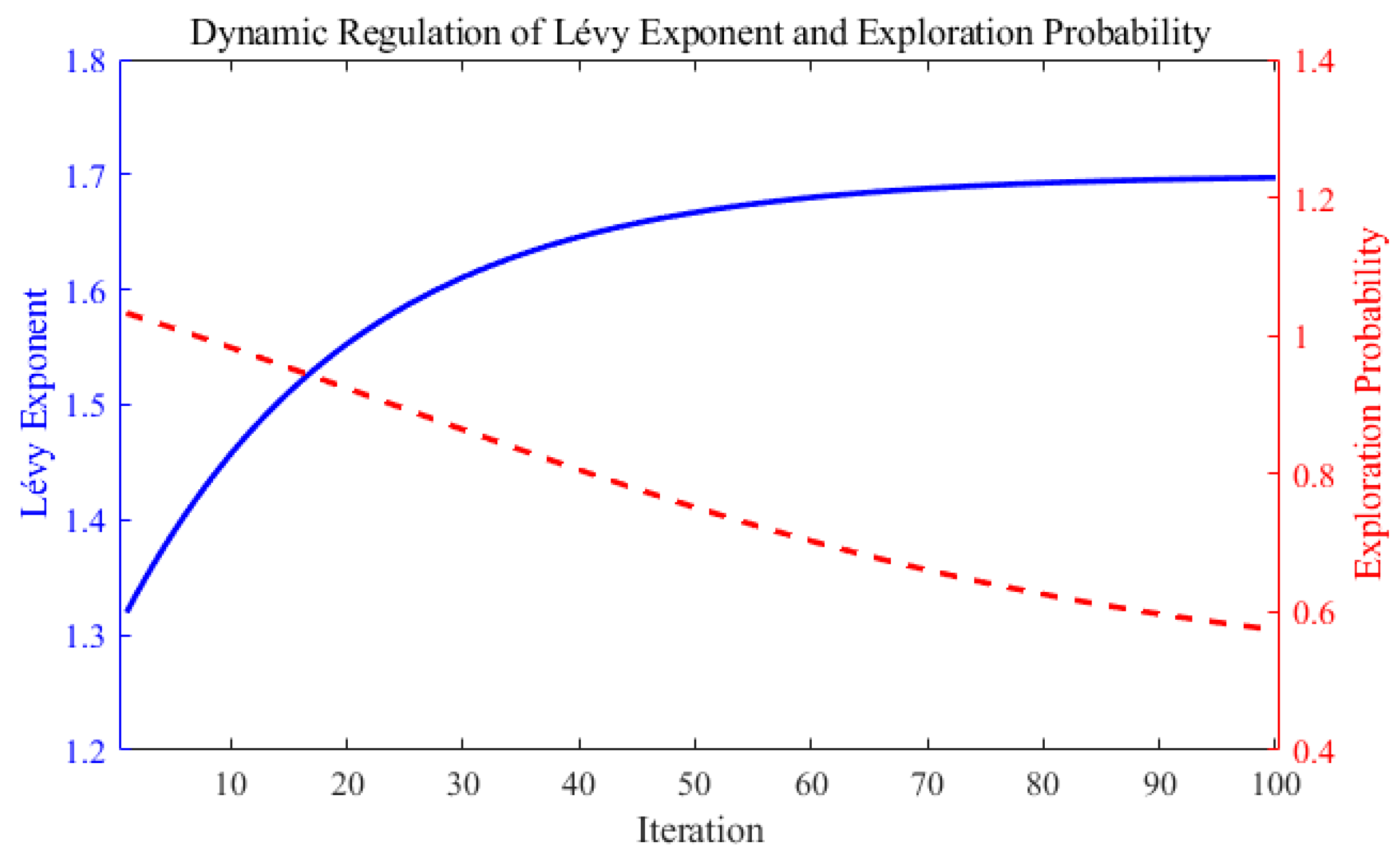
Based on the variation characteristics of the exploration probability function, this paper proposes a coordinated improvement of the whale fall step mechanism to systematically enhance the algorithm’s phase-wise control capability. This coordination mechanism adjusts the exploration probability to decrease nonlinearly with the number of iterations, keeping it relatively high during the early search stage to promote diversity, and gradually shifting toward the exploitation phase later on to improve local accuracy. Its mathematical expression is given as follows:
k T = k min + k max k min 1 + exp a T T max b
where k max = 1.3 and k min = 0.5 represent the initial maximum exploration probability and the minimum exploitation probability, respectively. The parameters a = 3 and b = 0.24 control the steepness and midpoint of the descent curve. This regulation strategy enables finer adjustment of exploration intensity for the population across different search stages.
Figure 8 compares the trend of exploration probability before and after applying the proposed improvement strategy. As shown in the figure, the original algorithm adopts a linear decay method, where the exploration probability decreases at a constant rate throughout the iteration process. The curve is monotonic and lacks adaptability to different search stages, making it difficult to dynamically balance between global exploration and local exploitation. In contrast, the improved sigmoid-shaped curve maintains a high exploration probability in the early stages, then gradually decreases and eventually stabilizes. This probability curve better supports the phased transition from early global exploration to later local exploitation during optimization, and the method proposed in this paper effectively balances both search efficiency and convergence quality.
Based on the improved trend of dynamic exploration probability, this paper further optimizes the whale fall step mechanism in a targeted manner. Specifically, the range of the step size adjustment factor r 7 is reduced from the original interval [0, 1] to [0.5, 1], increasing its expected value from 0.5 to 0.75. This significantly expands the initial jump range of the step size, thereby enhancing the algorithm’s capability to escape local optima in the early stages and strengthening its global search performance. In addition, the exponential decay coefficient C 2 is adjusted from 2.0 to 1.0, which slows down the decay of the step size. This allows relatively large perturbations to persist into the middle and later stages of the algorithm, maintaining population diversity and improving search precision. This optimization enables the whale fall step mechanism to perform more effectively across different stages of the algorithm: in the early phase, it supports larger jumps to quickly escape local optima; in the middle phase, it maintains moderate step sizes to ensure search diversity; and in the later phase, the gradually reduced step sizes promote stable convergence and improve the accuracy of the final solution.

2.3.4. Coordinated Regulation Advantages of Exploration Strategy and Lévy Index

The exploration probability function k T , innovatively designed in this paper, not only aligns closely with the improved whale fall step strategy but also forms a synergistic dual-control mechanism in conjunction with the optimized Lévy flight index α T . These two components, respectively, regulate behavioral tendencies and perturbation amplitudes during the search process. Through their joint modulation over the temporal dimension, the algorithm gains enhanced phase-adaptive capabilities. Figure 9 illustrates the collaborative regulation relationship between the exploration probability and the step-size control mechanism throughout the evolutionary process.
Specifically, k T determines whether an individual tends toward exploration or exploitation. It maintains a high value in the early phase to guide the population in broad global exploration, and then gradually decreases to shift the search toward local exploitation. Meanwhile, α T controls the jump length of the Lévy step. A smaller α corresponds to a larger step size, which facilitates rapid expansion of the search space in the early stage. As α increases, the step size gradually decreases, thereby enhancing the controllability of the perturbation scale in the later stage. The two components exhibit complementary evolutionary trends over time—one governs the search tendency, while the other adjusts the update scale. Their coordinated interaction throughout the optimization process enhances the overall global search capability and robustness of the algorithm.

2.3.5. Testing the Improved IBWO Algorithm

To evaluate the effectiveness and stability of the IBWO algorithm, two benchmark functions—Schwefel’s Problem 2.21 and the Generalized Penalized Function—are selected to assess the optimization capability of various algorithms on unimodal and multimodal test functions.
Schwefel’s Problem 2.21 is a typical unimodal function characterized by symmetry and flat gradient regions, often used to evaluate the local exploitation ability and convergence precision of optimization algorithms. Its global minimum is zero, located at the origin. However, due to the absence of significant gradient information near the optimal solution, algorithms may experience slow convergence, making this function suitable for testing robustness and local stability. The function’s landscape is illustrated in Figure 10, and its formula is given as
f x = max x i , 1 i 30 , 100 x i 100
Figure 10. Schwefel’s Problem 2.21 Test Function.
Sustainability 17 09746 g010
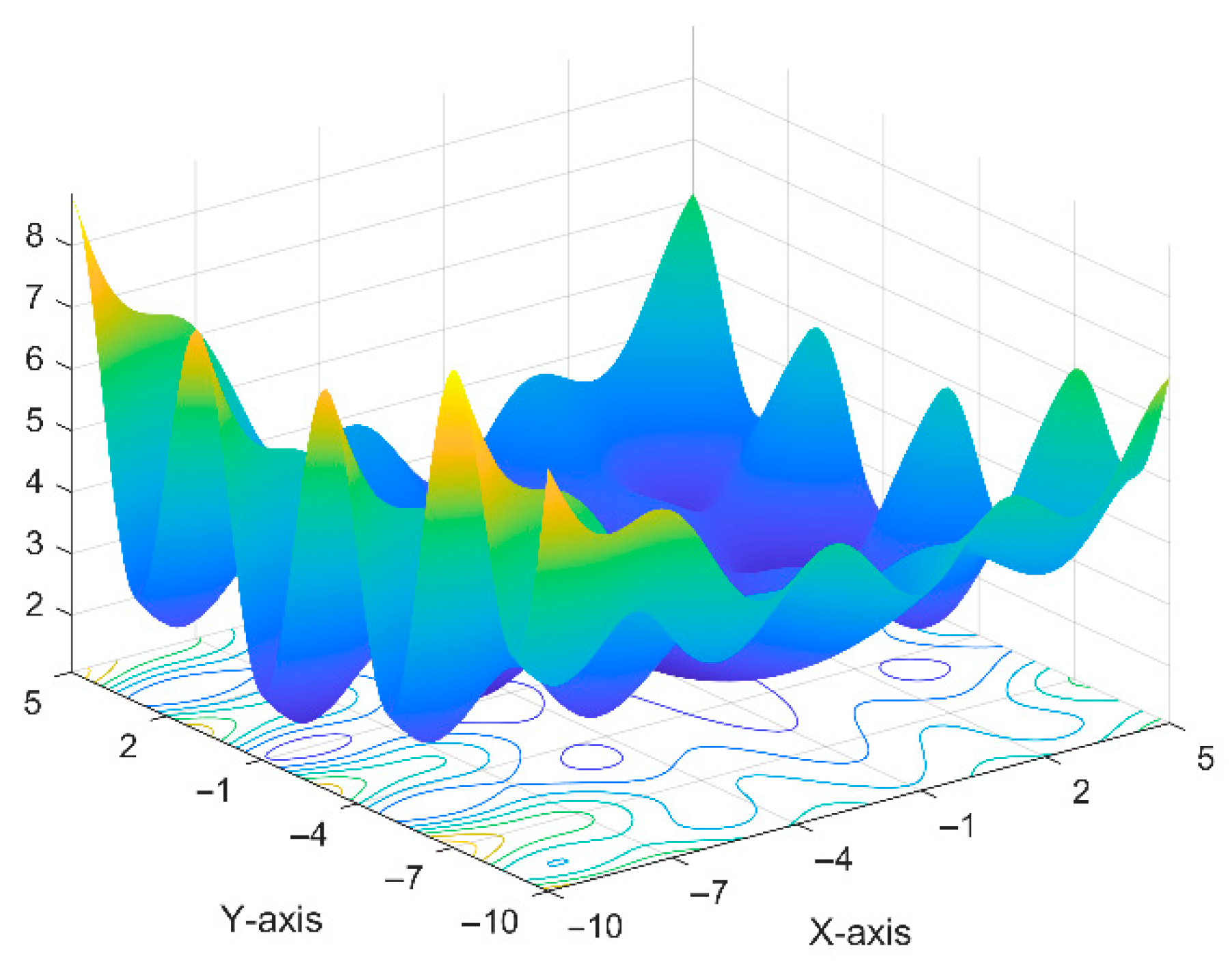
The Generalized Penalized Function is a highly complex multimodal nonlinear function, as shown in Figure 11. In Figure 10 and Figure 11, the colors of the function visualizations have no specific meaning and are used solely to enhance the visual appeal and clarity of the figures. It integrates sinusoidal perturbations with boundary penalty terms and is characterized by a large number of local optima and a complicated boundary structure, making it significantly more challenging to optimize. This function is commonly used to evaluate an algorithm’s global search capability, its ability to escape from local optima, and its robustness and adaptability in handling constrained boundaries. Let x = x 1 , x 2 , x d R d ; the function is defined as follows:
f x = π 30 10 sin 2 π y 1 + i = 1 29 y i 1 2 1 + 10 sin 2 π y i + 1 + y d 1 2 + i = 1 30 U x i , 10 , 100 , 4
where 50 x i 50 , and the variable transformation y i is computed as follows:
y i = 1 + x i + 1 4 , i = 1 , 2 , , d
The penalty function U x i , a , k , m is defined as
U x i , a , k , m = k x i a m 0 k x i a m i f   x i > a i f   x i a i f   x i < a
Figure 11. Generalized Penalized Function Test Function.
Sustainability 17 09746 g011
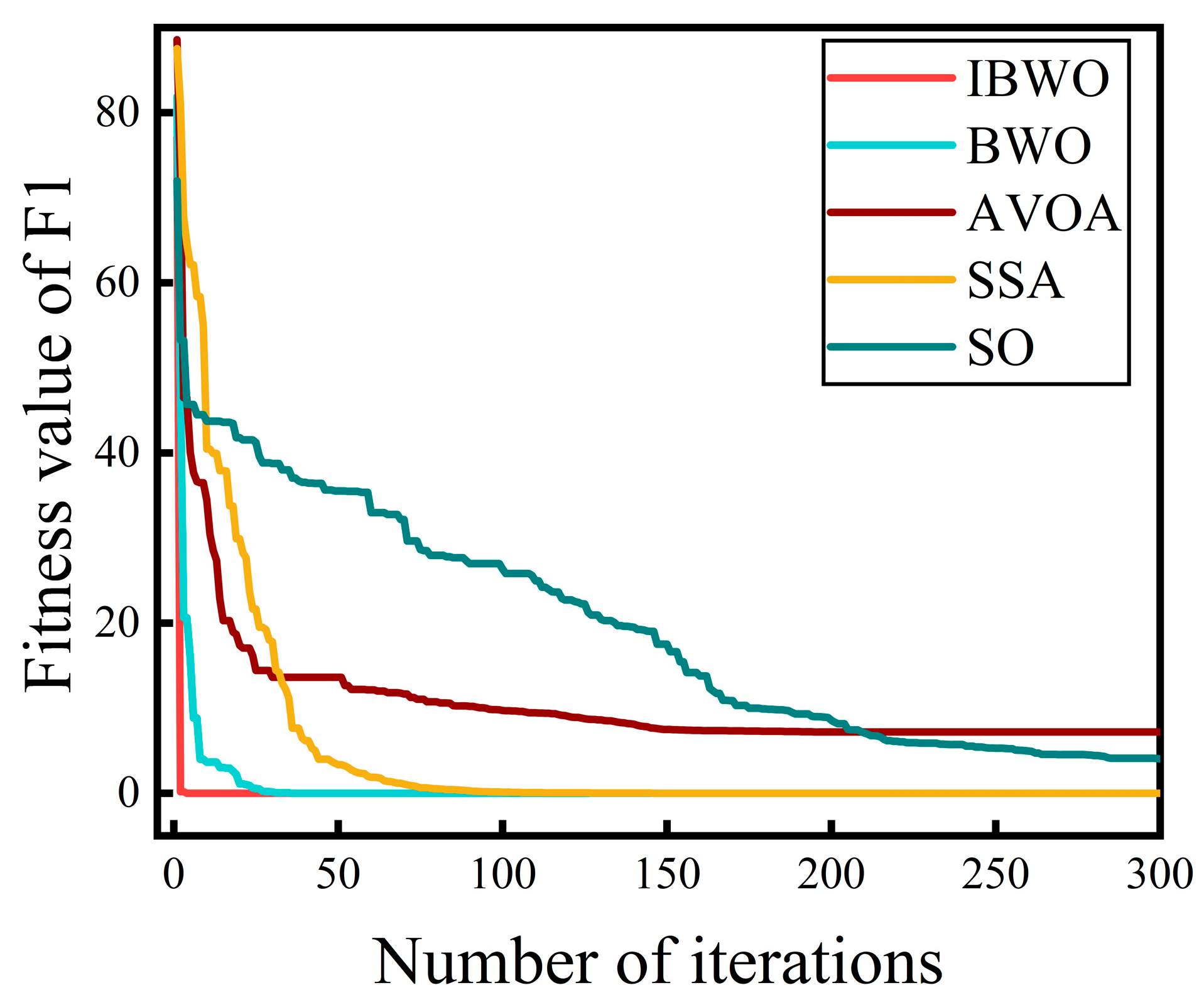
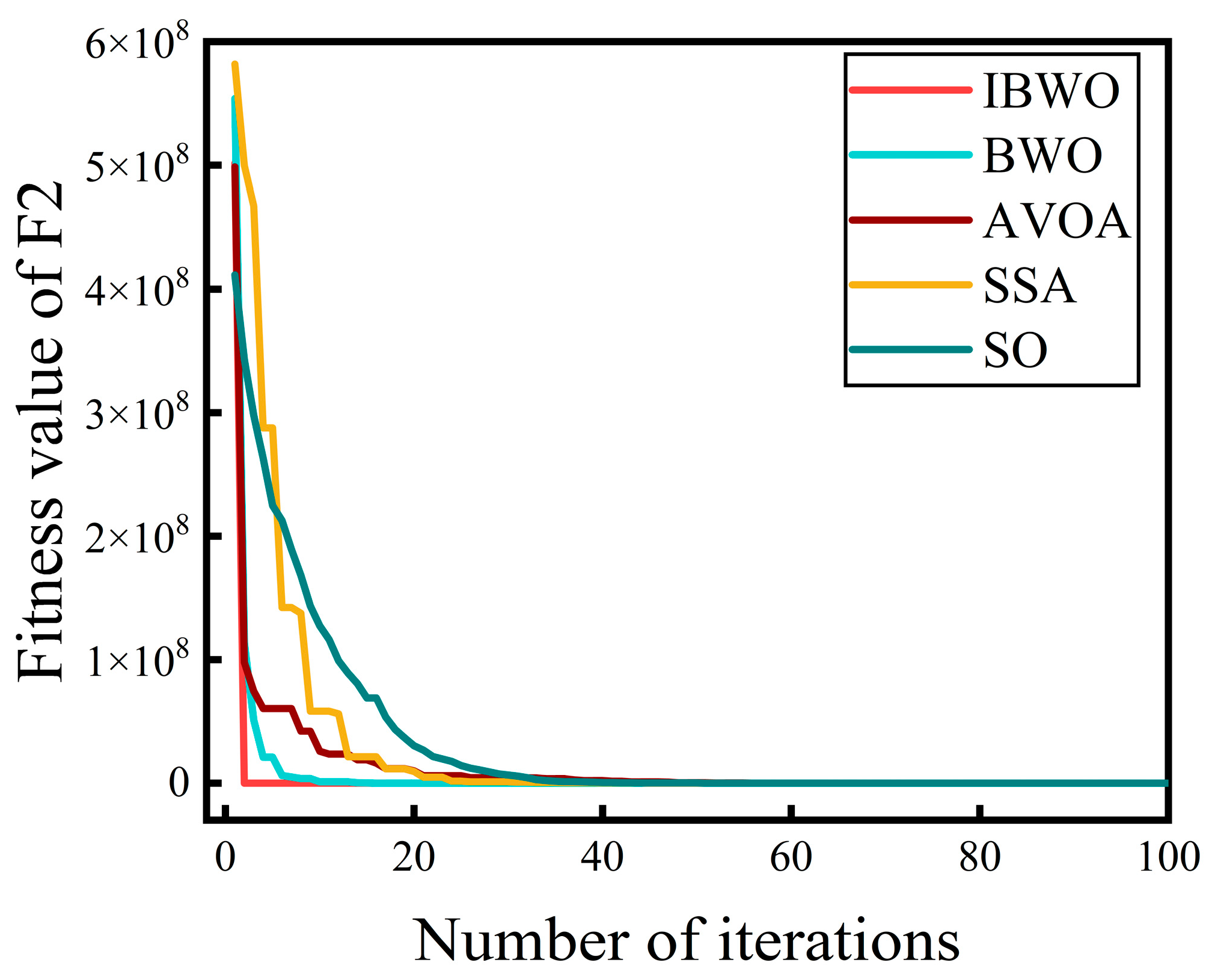
To evaluate the performance of the IBWO algorithm, comparisons are made with the standard BWO, African Vulture Optimization Algorithm (AVOA), Sparrow Search Algorithm (SSA), and Snake Optimizer (SO). All algorithms are configured with an initial population size of 50 and run for 300 iterations. The experimental results are presented in Table 4 and Table 5, while the iterative optimization processes of the two benchmark functions are illustrated in Figure 12 and Figure 13.
As shown in Figure 12, in the optimization task of the unimodal function F1 (Schwefel’s Problem 2.21), different algorithms exhibit significantly distinct convergence behaviors within 300 iterations. Leveraging a multi-phase collaborative control mechanism, the IBWO algorithm achieves a rapid and stable convergence process, with a sharp decline observed within the first 10 iterations. Among all compared algorithms, IBWO is the earliest to approach the optimal solution, demonstrating superior global search capability and convergence efficiency.
In contrast, the standard BWO algorithm shows slower convergence speed and lower accuracy than IBWO. Although it exhibits some ability to escape local optima, its overall performance remains insufficient, thus validating the effectiveness and necessity of the improvements introduced in IBWO.
Both AVOA and SSA show some initial decreasing trends. AVOA experiences a rapid decline in the early iterations but soon stagnates and becomes trapped in a local optimum, leading to poorer convergence accuracy and stability compared to IBWO. SSA shows a more gradual descent and a relatively stable convergence process, eventually approaching an optimal value close to that of IBWO, but its convergence efficiency remains inferior, indicating weaker overall optimization performance than IBWO.
The SO algorithm, due to the structural design of its search strategy, exhibits pronounced fluctuations during the early stages, with oscillations in individual updates and a lack of stable convergence. Only in the later stages does it show some convergence capability, but its final accuracy is still significantly lower than that of IBWO.
In summary, IBWO demonstrates the most stable performance on this function, successfully balancing convergence speed and solution precision, thus verifying its superior robustness and optimization capability for unimodal problems.
Figure 13 compares the convergence performance of each algorithm on the complex multimodal function F2 (Generalized Penalized Function). Since most algorithms converge within the first 100 iterations, only the first 100 iterations are plotted to more clearly illustrate the differences in convergence trends.
The IBWO algorithm exhibits a rapid descent in the early stages of iteration and approaches the optimal solution within 10 iterations, demonstrating excellent convergence speed. This performance is attributed to the multi-strategy collaborative control mechanism introduced in IBWO, which significantly enhances global search efficiency.
In contrast, although both SSA and SO are able to approximate the global optimum in the later stages, their optimization processes show noticeable fluctuations. In particular, SSA undergoes multiple abrupt transitions during the search, reflecting its high sensitivity to local extrema in complex search spaces. While SO ultimately achieves acceptable convergence accuracy, its early-stage convergence rate is relatively slow.
The AVOA and standard BWO algorithms exhibit a relatively stable convergence process overall, with better accuracy than SO and SSA, but still fall short of IBWO—especially in terms of convergence speed and stability. By comparison, the IBWO algorithm, when applied to complex high-dimensional nonlinear problems, not only converges faster but also effectively avoids local optima, showcasing superior global search capability and robustness over the compared algorithms.
Table 4 and Table 5 present the performance of five optimization algorithms on the benchmark test functions F1 and F2, respectively. Overall, IBWO demonstrates superior optimization capability, average performance, and stability across both functions, highlighting its adaptability and significant advantage over other methods for different types of optimization problems.
Specifically, for the F1 function, both IBWO and BWO successfully reach the theoretical optimal value of 0, indicating strong local exploitation and precise objective approximation capabilities. In contrast, the optimal results for AVOA, SO, and SSA are 7.2146, 4.0316, and 0.0007, respectively. Among these, SO and AVOA show substantial deviation from the optimal value, suggesting weaker global search abilities and lower overall efficiency in solving unimodal problems. Although SSA does not reach the optimum, its result is relatively close, indicating relatively strong local optimization capabilities.
The average value reflects the overall quality of solutions obtained by an algorithm. Unlike the optimal value, it effectively measures an algorithm’s robustness in complex search spaces, particularly in high-dimensional functions. A lower average value indicates greater reliability. As shown in the tables, IBWO achieves the best average value of 0.2582, significantly outperforming the others. While BWO performs well, its accuracy is slightly inferior to IBWO. SSA and AVOA report average values of 4.7188 and 10.6977, indicating high fluctuation and a tendency to get trapped in local regions. SO performs the worst with an average of 19.2316, revealing a lack of stability in its search process.
The standard deviation measures the variability of solutions across multiple runs and is a key indicator of stability and robustness. A lower standard deviation suggests consistent results under different initial conditions. IBWO reports the smallest standard deviation at 4.4499, indicating the most stable optimization process. BWO and AVOA have standard deviations of 5.8163 and 8.3188, respectively, showing higher variability due to less refined search control strategies. SSA and SO have standard deviations exceeding 13, indicating significant solution fluctuations and susceptibility to local traps or ineffective perturbation control. Overall, IBWO exhibits strong stability and adaptability to complex problems.
In the more challenging F2 function, IBWO achieves the lowest optimal value of 4.64 × 10⁻²⁴, demonstrating excellent global search capability and precision. In comparison, BWO and SSA attain optimal values of 1.18 × 10⁻⁵ and 3.71 × 10⁻², showing slightly lower precision. AVOA and SO obtain optimal results of 0.6306 and 4.4151, respectively, which deviate significantly from the global optimum, indicating a lack of effective mechanisms to escape local optima in complex nonlinear problems.
Regarding the average value on this high-dimensional complex function, IBWO reports 1.67 × 10⁶, significantly outperforming the other algorithms and indicating its ability not only to locate the global optimum but also to consistently obtain high-quality solutions across multiple runs. BWO and AVOA record average values of 2.61 × 10⁶ and 4.28 × 10⁶, showing noticeable gaps. SSA and SO yield average values of 9.77 × 10⁶ and 1.07 × 10⁷, respectively, deviating substantially from the optimal result and revealing a vulnerability to local minima and initialization sensitivity, thereby reducing overall search reliability.
Finally, IBWO achieves the lowest standard deviation, 2.89 × 10⁷, among all algorithms, reflecting its stable optimization behavior. BWO and AVOA report standard deviations of 3.27 × 10⁷ and 3.06 × 10⁷, indicating moderate variability. SSA and SO show significantly higher standard deviations of 5.83 × 10⁷ and 4.71 × 10⁷, respectively, further underscoring their lack of robustness in complex problem settings. Taken together, IBWO exhibits clear advantages in both average performance and stability, validating its reliability and generalization capacity in solving high-dimensional complex optimization problems.

2.3.6. Ablation Study of IBWO Algorithm

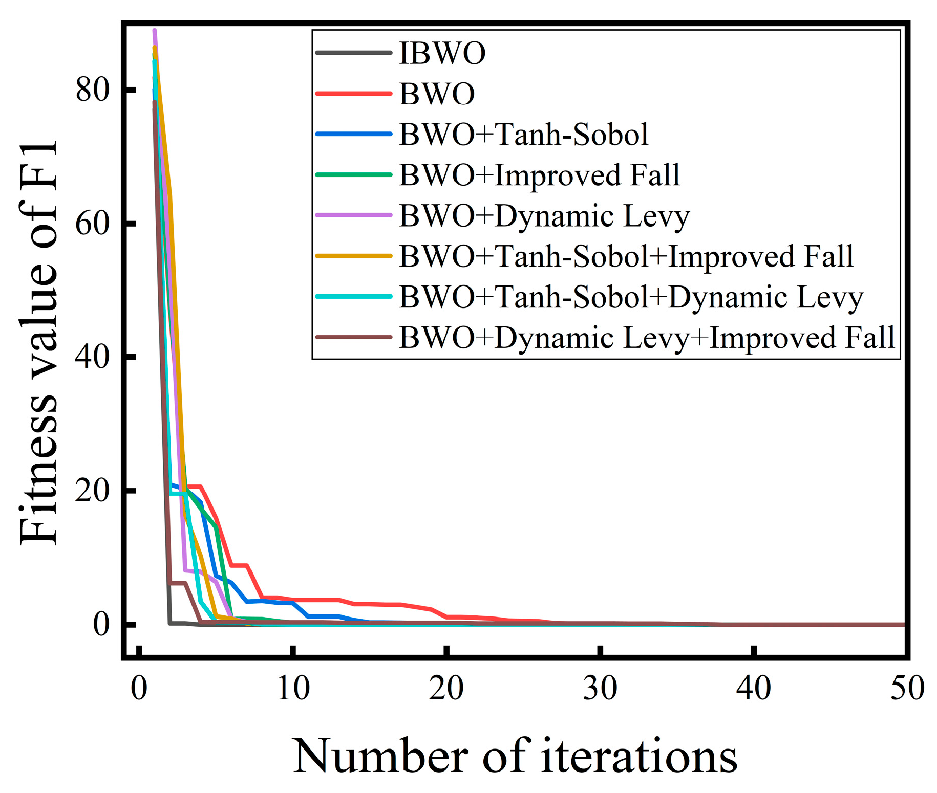
To further investigate the independent contributions of each strategy in the proposed IBWO algorithm, we designed and conducted ablation experiments. In this experiment, the Tanh-Sobol Population Initialization, Dynamic Lévy Flight Mechanism, and Improved Whale Fall Step Strategy were progressively removed from the algorithm to evaluate their specific impact on the overall optimization performance. Figure 14 shows the performance of each strategy combination on the Schwefel’s Problem 2.21 function, and Table 6 lists the optimal values, mean values, and standard deviation statistics obtained under different combinations.
The Schwefel’s Problem 2.21 function is a commonly used single-peaked test function in global optimization studies and is highly sensitive to variable disturbances, making it easier to evaluate the impact of different strategies on optimization performance. Figure 14 presents the convergence curves of the IBWO algorithm on this function with different module combinations. By comparing, it can be initially observed that as each improvement strategy is progressively introduced, the algorithm’s optimization capability gradually increases.
Among these, BWO+Tanh-Sobol and BWO+Improved Fall both enhanced the optimization performance of the base algorithm to varying degrees. Tanh-Sobol improved the search starting point by generating a more uniform initial population, but its subsequent search strategy remained the same as the standard BWO, with limited improvement. In contrast, Improved Fall significantly enhanced global search capability by improving the jump step mechanism. The combined BWO+Tanh-Sobol+Improved Fall scheme integrates both initialization optimization and search enhancement strategies, showing superior performance in convergence speed and accuracy.
Of all the improvements, the performance boost from the Dynamic Lévy flight mechanism was the most significant. This is due to its ability to dynamically adjust the jump step size during the search phase, thereby improving search efficiency and reducing the risk of getting stuck in local optima. Furthermore, when Dynamic Lévy flight was combined with Tanh-Sobol initialization and the Improved Whale Fall Step Strategy, the algorithm demonstrated stronger advantages in stability and global search ability, ultimately forming the complete IBWO algorithm.
It is worth noting that the standard deviations of BWO+Tanh-Sobol and BWO+Tanh-Sobol+Dynamic Lévy in Table 6 are similar and both small, yet the optimization processes behind them differ significantly. As shown in Figure 14, BWO+Tanh-Sobol tends to get trapped in local optima, leading to a concentration of results and a small standard deviation, but with relatively low overall accuracy. On the other hand, BWO+Tanh-Sobol+Dynamic Lévy maintains output stability while having a stronger ability to escape local optima, resulting in better convergence and indicating superior overall optimization performance.

2.4. Dilated BiGRU

2.4.1. GRU

GRU retains the core concept of the gating mechanism and achieves selective update and retention of hidden state information through the collaborative effect of the update gate and the reset gate, as illustrated in Figure 15. Specifically, the state update process of GRU at each time step can be described as follows:
  • Computation of the Update Gate: The update gate determines how much of the previous hidden state should be retained in the current time step. Its output ranges between 0 and 1; a larger value indicates more past information is preserved, while a smaller value suggests greater reliance on the current input. The computation is formulated as follows:
    z t = σ W z , h t 1 , x t + b z
    where W z and b z are the weight matrix and bias vector, respectively; h t 1 is the hidden state from the previous time step; x t is the current input; and σ denotes the Sigmoid activation function.
  • Computation of the Reset Gate: The reset gate determines the extent to which the previous hidden state should be forgotten. When the reset gate outputs a value close to 0, the network tends to “forget” the information from the previous time step and relies solely on the current input. Conversely, an output close to 1 leads to more retention of the previous hidden state. The formula is as follows:
    r t = σ W r h t 1 , x t + b r
    where W r and b r are the weight matrix and bias vector of the reset gate.
  • Computation of the Candidate Hidden State: The GRU uses the reset gate to control the extent to which the previous hidden state contributes to the current candidate hidden state. The candidate hidden state is computed as
    h ˜ t = tanh W r t h t 1 , x t + b
    where r t h t 1 represents the element-wise combination of the previous hidden state h t 1 and the reset gate r t , which controls the degree of influence from past information. W and b denote the parameter matrix and bias vector, respectively.
  • Update of the Hidden State: The update gate z t is used to compute the current hidden state h t as follows:
    h t = z t h t 1 + 1 z t h ˜ t
    where z t h t 1 represents the preserved historical information, while 1 z t h ˜ t corresponds to the newly introduced information. This formula determines that the current hidden state retains part of the previous time step’s information while incorporating new information derived from the current input.
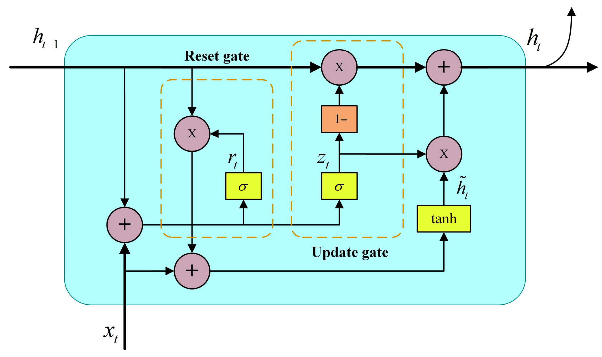
Figure 15. GRU Unit Structure.
Sustainability 17 09746 g015
In the model structure diagram shown in Figure 15, the colors have no specific meaning and are used only to distinguish different structural parts for better visualization. The dashed areas are for aesthetic purposes. Compared with the complex multi-gate architecture of LSTM, the dual-gate design of GRU is more compact, omitting the separate memory cell. This results in significantly fewer parameters and reduced computational overhead. Furthermore, GRU directly updates information using the hidden state, thereby avoiding additional interference during state transmission and improving training stability and convergence speed.

2.4.2. BiGRU

Traditional unidirectional GRUs exhibit certain limitations in capturing long-term dependencies and maintaining contextual completeness, making it difficult to fully exploit bidirectional temporal features. To address this issue, the BiGRU was introduced. Its bidirectional architecture enables the model to perceive information from both past and future time steps simultaneously, thereby enhancing its understanding of the overall structure of the sequence.
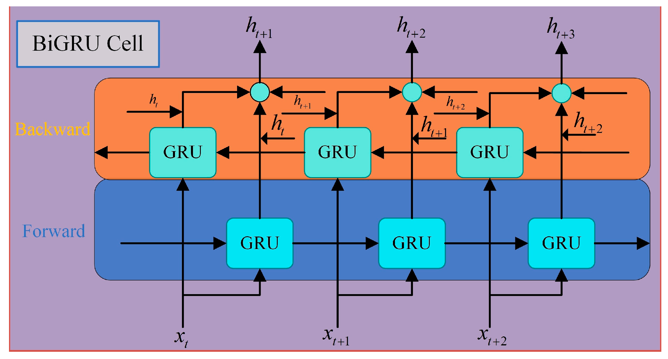
BiGRU consists of two GRU networks operating in opposite directions, as illustrated in Figure 16. The core idea is to extend the standard GRU framework by introducing a pair of independent recurrent units that perform state updates in the forward and backward directions of the time sequence, respectively. The orange area represents the backward propagation part, and the blue area corresponds to the forward propagation part, whereas the other colors are included merely for aesthetic purposes. Specifically, at each time step t , each GRU unit receives the current input x t and the previous hidden state from its corresponding direction and computes the current state through a gating mechanism. Assuming the input sequence is X = x 1 , x 2 , , x n , BiGRU generates two parallel hidden state sequences:
  • The forward GRU processes the input sequence x 1 x n , producing the forward hidden state sequence h 1 , h 2 , , h n .
  • The backward GRU processes the reversed sequence x n x 1 , yielding the backward hidden state sequence h 1 , h 2 , , h n .
At each time step, the final representation h t = h t ; h t is formed by concatenating the hidden states from both directions. This bidirectional aggregation enables the model to simultaneously incorporate contextual information from both the past and future, significantly enhancing its ability to capture global semantic dependencies.
Figure 16. Structure of the BiGRU Cell.
Sustainability 17 09746 g016
While BiGRU generates richer sequence representations compared to GRU, it also inherits the structural simplicity and computational efficiency of the GRU. Compared with bidirectional LSTM, BiGRU features lower parameter overhead and faster training speed, thereby achieving a favorable balance between modeling capacity and resource consumption.

2.4.3. Dilated-BiGRU

The conventional BiGRU updates its state through adjacent time steps, which can lead to information degradation and gradient vanishing when dealing with long sequences or complex high-dimensional data. This makes it difficult to capture dependencies across distant time steps. To address this issue, this paper proposes a BiGRU model with a dilation mechanism: Dilated BiGRU. By introducing a fixed dilation step, the model enables each BiGRU unit to access temporally distant data points, thereby enhancing its ability to model long-range dependencies and expanding the temporal receptive field, all while keeping the number of parameters low.
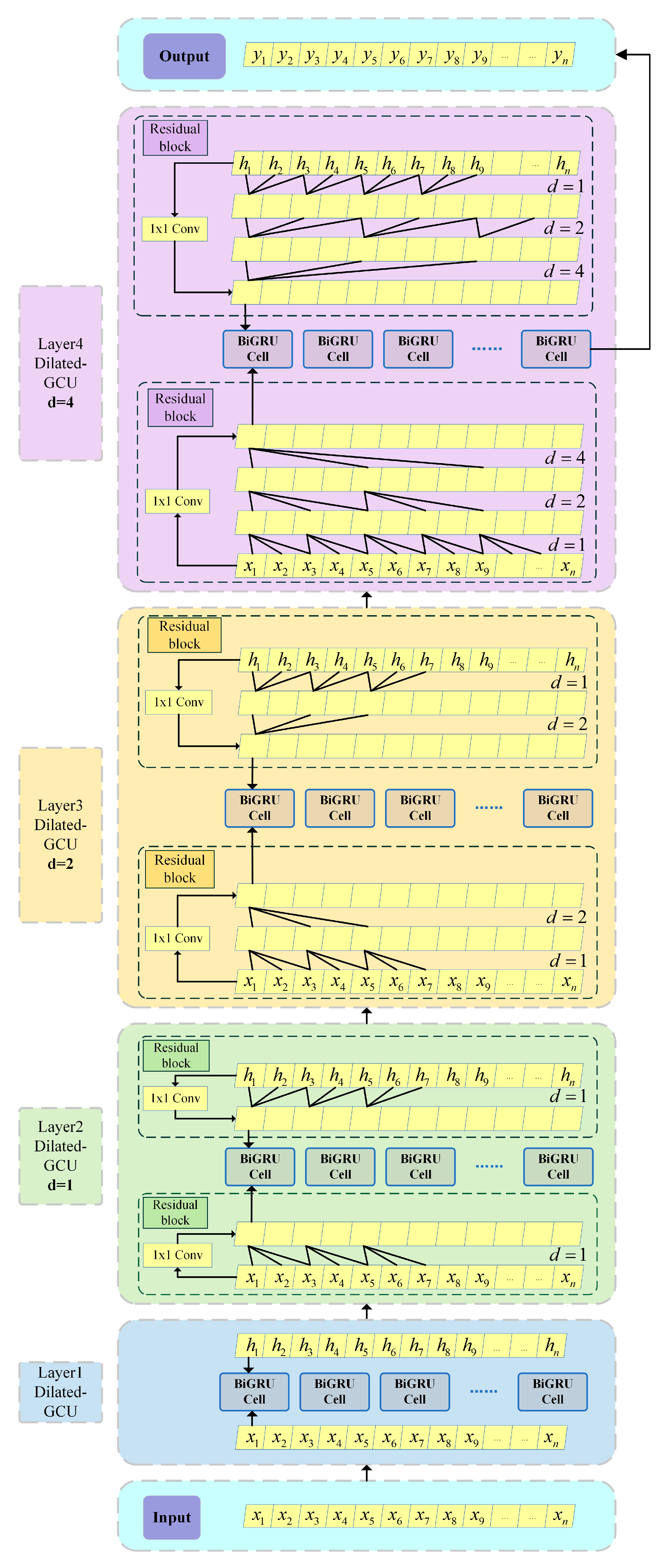
Unlike the standard BiGRU, the Dilated BiGRU adopts a skip-step state update strategy, enabling BiGRU units to access hidden states from more distant time steps. As illustrated in Figure 17, a one-dimensional dilated convolution operation is applied to the original input sequence. The dark blue, green, orange, and purple areas in the figure correspond to the four layers of the Dilated-GRU structure, each performing more refined feature extraction than the previous one. The darker dashed lines indicate the residual connection structure, which facilitates cross-layer information transfer and feature preservation. Other colors and dashed lines are used solely to enhance the visual clarity of the figure. By setting different dilation rates, the model can capture the correlation between the current input and distant historical information, thus providing the subsequent BiGRU units with richer and more hierarchical contextual features. The dilated convolution is formally defined as follows:
F ( t ) = ( x d f ) ( t ) = i = 0 u 1 f ( i ) x t p i
x denotes the input sequence, represents the convolution operation, d is the dilation factor, u is the kernel size, f i refers to the i-th element of the convolution kernel, and x t p i is the corresponding input element. This operation enlarges the receptive field of the model without increasing the number of parameters, making it particularly suitable for modeling complex sequences with periodicity or non-stationarity.
In addition to incorporating the dilation mechanism into the input sequence, this study further integrates a one-dimensional dilated convolution operation into the transmission path of the hidden state h t . This allows the model, during the state update at each time step, to incorporate hidden state information h t d from more distant time points. Such a mechanism enhances the model’s capacity for long-range structure perception, helps mitigate gradient vanishing, and improves training stability.
To further enhance the fusion of multi-scale features in the dilated path, a residual connection mechanism is introduced into the Dilated BiGRU architecture. Specifically, a convolution operation is embedded within the dilated connection path to achieve a linear integration of the original input and long-distance state features. This structure not only improves the representational capacity of information across time steps but also constructs a stable information compensation path, thereby maintaining the integrity of feature representation while enhancing the model’s efficiency in capturing long-term dependencies. The introduction of residual connections further improves gradient propagation in deep architectures and contributes to overall training stability.
In summary, based on the bidirectional sequence modeling and dilated connection mechanisms, Dilated BiGRU enhances its modeling capacity for long sequences and complex feature relationships through the introduction of multi-scale information fusion. The dilated connection broadens the temporal receptive field while maintaining a relatively shallow model depth, thereby enhancing the representation of long-range dependencies. Experimental results demonstrate its robust performance and strong generalization capabilities.
Figure 17. Structure of Dilated BiGRU.
Sustainability 17 09746 g017

2.5. Model Construction: Steps and Architecture

In this section, the modeling process and architectural details of the proposed forecasting model are presented. The components of the model have been elaborated in previous sections. Based on these components, the proposed model is named IBWO-Dilated BiGRU, and its structural schematic is illustrated in Figure 18.
From Figure 18, it can be observed that the complete forecasting pipeline can be divided into three parts according to their functional roles: the Feature Engineering Part, the IBWO-based Parameter Optimization Part, and the Dilated BiGRU Forecasting Model Part, which generates the final prediction results. The following description proceeds chronologically. Except for the parts consistent with Figure 17, the colored areas in Figure 18 are used solely for aesthetic purposes and have no specific meaning.
Part (a), Feature Engineering Part:
  • Perform Spearman correlation analysis on the high-dimensional raw dataset to evaluate the correlation strength between each feature and the load target.
  • For features with low correlation, low-frequency trend components are retained to enhance model training and improve forecasting accuracy.
  • For features with high correlation, secondary modal decomposition is applied to generate refined training data. After VMD, the low-frequency components are fused with the outputs from step 2 to form the low-frequency portion of the new dataset; the high-frequency components are stored separately to serve as the high-frequency data of the new dataset.
  • The data processed through feature engineering is split in a 70%:30% ratio to form the training set and testing set for the model.
Part (b), IBWO-based Parameter Optimization Part:
  • The Beluga Whale Optimization algorithm is enhanced as described in the earlier Section 2.3, resulting in the improved version named IBWO.
  • The number of hidden units, batch size, and learning rate are selected as the optimization targets.
  • The optimal solution set obtained through IBWO is fed into the forecasting model to complete hyperparameter optimization, thereby improving predictive accuracy.
Part (c), Dilated BiGRU Forecasting Model Part:
  • The forecasting model is constructed based on the method introduced in the earlier Section 2.4.
  • The optimal hyperparameter set obtained in Part (b) is applied to the appropriate positions in the model.
  • The model is trained using the training set from Part (a).
  • The model’s prediction performance is evaluated using the testing set from Part (a).

3. Results

To objectively evaluate the predictive performance of the IBWO-Dilated BiGRU model, this study designs a systematic and rigorous experimental framework. All experiments in this section utilize the same dataset, specifically the original power load dataset processed through the feature engineering procedures outlined earlier. The experiments first compare the performance of several classical recurrent neural network models, including RNN, LSTM, GRU, BiLSTM, and BiGRU. Subsequently, the Dilated module is introduced into the best-performing model to assess its impact on predictive capability, alongside a comparison of performance changes in other models when the same module is integrated. Finally, by analyzing the enhancement effects of various optimization algorithms on the Dilated BiGRU, the results verify that the proposed IBWO algorithm significantly improves the forecasting performance of the model. The experiments related to the optimization algorithms were conducted using MATLAB R2023a, while the predictive modeling part was implemented in the PyCharm development environment with Python 3.9.

3.1. Performance Evaluation Metrics

To evaluate the performance of the proposed forecasting model, it is essential to adopt standardized and representative evaluation metrics to ensure the objectivity of comparison results. In this study, three widely used metrics in time series forecasting tasks are selected—Root Mean Square Error (RMSE), Coefficient of Determination (R2), and Mean Absolute Error (MAE)—to comprehensively assess the predictive performance of the model from multiple perspectives.
Specifically, the RMSE reflects the overall prediction accuracy of the model—a lower value indicates smaller fitting errors and thus more accurate predictions. Its unit is consistent with that of the original load data, namely megawatts (MW). The R2 metric evaluates the model’s explanatory power for the predicted data, ranging from 0 to 1, with values closer to 1 indicating better fitting performance. MAE measures the average absolute deviation between predicted and actual values, with lower values signifying closer alignment with real observations; its unit is also megawatts (MW). In all subsequent experimental analyses, the same unit convention is followed and not repeatedly indicated. Together, these three metrics provide a comprehensive evaluation of model effectiveness in time series forecasting tasks. The mathematical definitions are presented as follows:
R M S E = 1 n i = 1 n ( y i y ^ i ) 2
R 2 = 1 i = 1 n ( y i y ^ i ) 2 i = 1 n ( y i y ¯ ) 2
M A E = 1 n i = 1 n y i y ^ i
where y i denotes the actual value, y ^ i is the predicted value, y ¯ represents the mean of actual values, and n is the number of samples.

3.2. Baseline Prediction Models

Choosing an appropriate baseline model is the first and crucial step in predictive modeling, as this choice significantly influences prediction accuracy. In this study, we selected a variety of representative predictive models for comparative experiments, covering statistical methods, traditional machine learning methods, ensemble learning methods, and deep learning models based on Recurrent Neural Networks. These models each have distinct advantages in time series modeling, capturing nonlinear relationships, and extracting multi-scale features. Specifically, the models evaluated include: ARIMA, SVR, RF, the ensemble learning method XGBoost, and five typical RNN variants: RNN, LSTM, GRU, BiLSTM, and BiGRU.
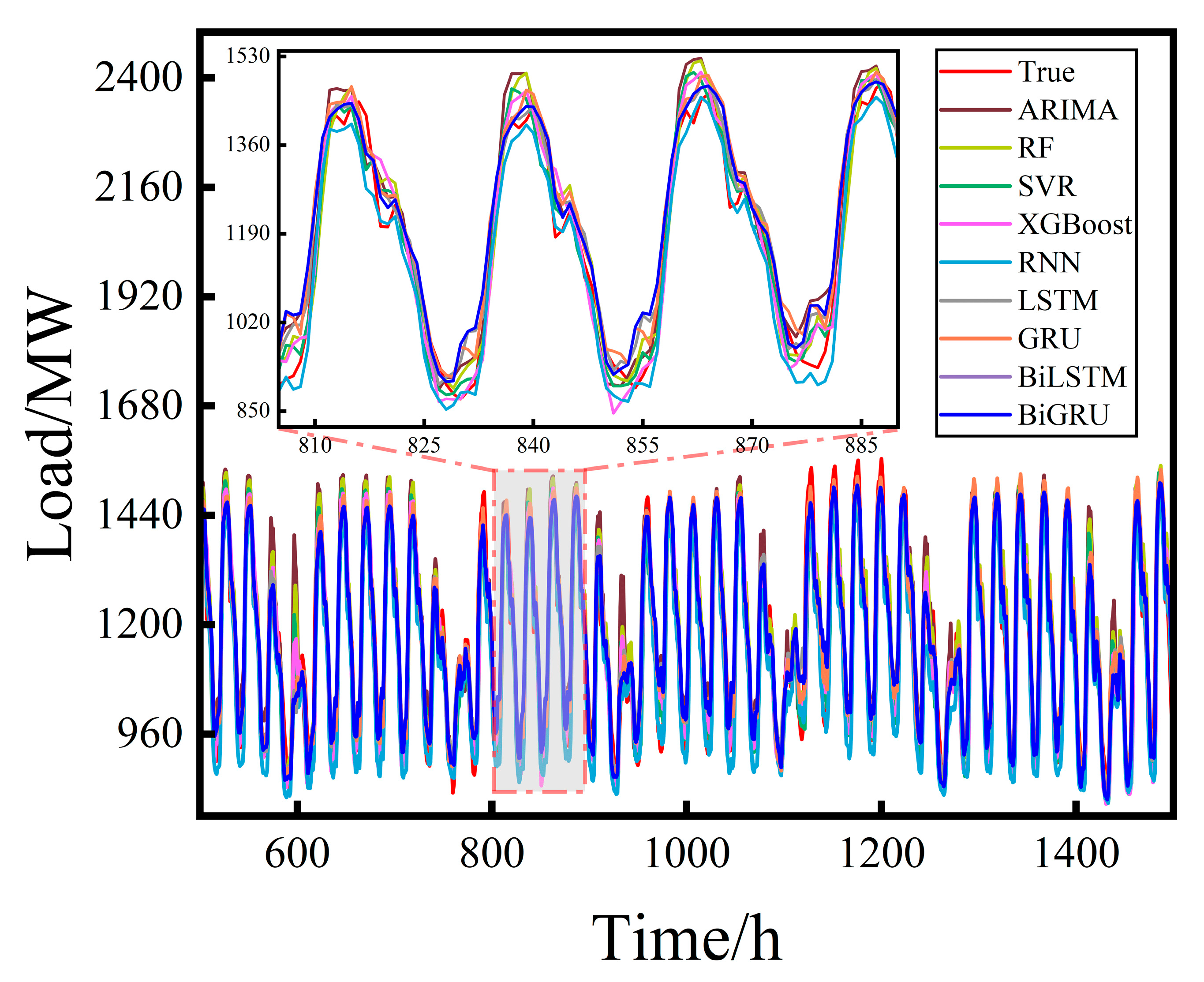
By comparing the prediction performance of each model on the same dataset and analyzing the results using the defined evaluation metrics, the model with the best performance is ultimately selected as the foundation for subsequent enhancements. The corresponding experimental results are presented in Figure 19 and Figure 20, and Table 7.
Figure 19 presents the fitting performance of nine representative baseline models in the electricity load forecasting task. The horizontal axis represents time (unit: hours), while the vertical axis denotes load values (unit: MW). To better highlight the fitting details within specific time intervals, the figure also includes a magnified view of a local region, which is indicated by the red dashed area. The red dashed lines are purely for aesthetic purposes, and the same axis definitions and design principle are applied to the subsequent figures.
In the figure, the red curve indicates the actual load, while curves in other colors correspond to the predictions generated by different models. The overall trend shows that deep learning models based on Recurrent Neural Networks can effectively capture the periodic patterns in load data, demonstrating strong time series modeling capabilities. The zoomed-in view further reveals the response differences among the models in the load fluctuation regions, helping to more thoroughly assess their fitting accuracy. The results indicate that the BiGRU model exhibits superior fitting performance over most time intervals, with smaller errors between the predicted and actual curves, smooth fitting, and rapid response to peak and valley changes. BiLSTM and GRU follow closely behind, also showing good modeling capabilities.
Regarding the fitting performance of traditional statistical and machine learning methods, models such as ARIMA, SVR, RF, and XGBoost are able to roughly track the actual load curve in terms of overall trends. However, they perform relatively poorly in capturing local abrupt changes and high-frequency fluctuations. The predicted curves often show shifts in the peak and valley regions, making it difficult to accurately reflect the short-term dynamic characteristics of the load. This highlights, to some extent, the limitations of traditional models in handling complex, nonlinear time series structures.
Comparatively, models equipped with gating mechanisms—such as LSTM, GRU, BiLSTM, and BiGRU—demonstrate enhanced memory capabilities, producing predictions that are more closely aligned with actual values. Further examination of the magnified regions reveals that when the load sequence undergoes sharp fluctuations or trend reversals (e.g., from rising to falling), the BiGRU model responds in a smoother and more stable manner. Its predicted trends closely mirror the actual load trajectory, reflecting a stronger ability to perceive global temporal patterns.
Such a stable response pattern contributes to the model’s robustness under complex and dynamic conditions and reduces the adverse impact of prediction errors on dispatch systems, thereby better fulfilling the real-world requirements for continuity and controllability in engineering applications. In conclusion, the BiGRU model demonstrates outstanding performance in both fitting precision and trend-capturing capability, which is one of the key reasons it was selected as the foundational model for subsequent improvements in this study.
Figure 20 presents the performance of various models across three evaluation metrics: RMSE, R2, and MAE. This visualization facilitates an intuitive comparison and comprehensive analysis of the predictive capabilities of each model. The results are displayed using bar charts, where the horizontal axis represents the selected prediction models, with different colors used to enhance readability. The legend specifies the names of the corresponding models, while the vertical axis denotes the specific values for each performance metric.
By comparing the height of the bars, one can clearly identify the strengths and weaknesses of each model across different evaluation dimensions. This visual comparison aids in assessing the overall forecasting capability of each model.
According to the results shown in Figure 20 and Table 7, the BiGRU model demonstrates the best overall performance across all evaluation metrics. In terms of RMSE, BiGRU achieves a value of 52.3161, which is significantly lower than those of other models, indicating higher prediction accuracy and smaller forecasting error. Regarding the R2, BiGRU reaches 0.9132, substantially outperforming the other models, reflecting its superior data-fitting capability. Moreover, it attains the lowest MAE value of 39.8785, further highlighting its advantage in both prediction accuracy and stability.
The performance of the baseline comparison models is relatively inferior, primarily due to the limitations of their modeling capabilities. ARIMA, as a typical linear time series method, struggles to effectively capture the nonlinear characteristics in electricity load data. While SVR has some nonlinear modeling capabilities, it falls short in handling the long-term dependencies in sequential data. RF is relatively robust in predicting overall trends, but its ability to fit local fluctuations is limited, often resulting in underfitting. Although XGBoost shows good fitting performance in certain segments, its overall stability is not on par with deep learning models, and it struggles to effectively capture the temporal structure and potential dependencies between input features.
While gated recurrent architectures such as LSTM, GRU, and BiLSTM enhance the modeling of temporal dependencies, they still fall slightly short of BiGRU in terms of precision and error minimization. Among the RNN-based models, BiGRU stands out due to its significantly better fitting performance and quantitative metrics, making it the optimal foundation for further model improvements. Based on the comparative analysis of the fitted curves and evaluation indicators, this paper ultimately selects BiGRU as the foundational architecture for subsequent optimization model design.

3.3. Validation Experiments for Dilated BiGRU

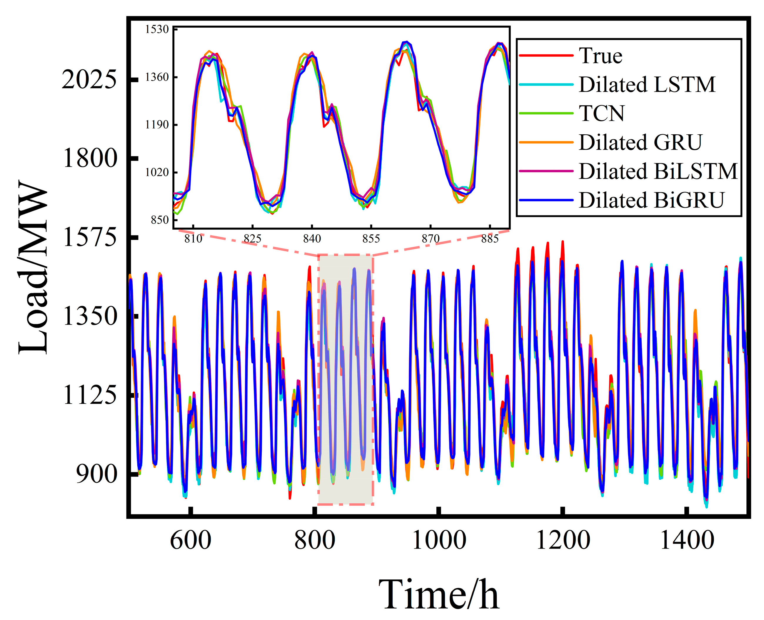
To evaluate the effectiveness of the proposed Dilated architecture in enhancing the accuracy of load forecasting, a series of controlled experiments were conducted. Specifically, the Dilated mechanism was integrated into LSTM, GRU, BiLSTM, and BiGRU models, resulting in improved variants named Dilated-LSTM, Dilated-GRU, Dilated-BiLSTM, and Dilated BiGRU, respectively. In addition, the Temporal Convolutional Network (TCN) was included as a baseline for comparison. The relevant experimental results are illustrated in Figure 21 and Figure 22, and Table 8.
Figure 21 illustrates the fitting performance of various recurrent neural network structures enhanced with the Dilated module in the load forecasting task. From the overall trend, all models demonstrate a good capacity to capture the periodic fluctuations of load data. However, substantial differences remain in the details among models. Based on the figure, two key conclusions can be summarized:
  • Dilated BiGRU exhibits the best performance: Its fitting curve closely matches the actual values, particularly in regions with sharp load fluctuations. It responds more smoothly and accurately, demonstrating superior trend-tracking capability and forecasting precision. Compared with it, Dilated-BiLSTM shows larger deviations in detailed regions and lacks stability. Dilated-GRU and Dilated-LSTM suffer from delayed responses and amplified errors during periods of abrupt change. Although the TCN model performs well in tracking the global trend, it lags behind Dilated BiGRU in terms of responsiveness and fitting accuracy at local turning points.
  • The Dilated module enhances overall model fitting performance: As shown in the figure, all models embedded with the Dilated mechanism produce smoother forecasting curves in areas of significant load variation. These curves are closer to the actual values compared to their original counterparts, revealing stronger fitting characteristics. This validates the advantages of the Dilated module in capturing long-term dependencies and mitigating short-term disturbances.
As shown in Figure 22 and Table 8, all model variants incorporating the Dilated module exhibit consistently superior forecasting performance compared to their original counterparts. Specifically, the RMSE, R2, and MAE of the Dilated-LSTM model are 52.9719, 0.9180, and 40.5714, respectively, indicating a slight improvement in performance. The TCN model, by leveraging its dilated convolutional mechanism to deepen representation capacity, performs marginally better than the Dilated-LSTM in most metrics. The Dilated-GRU model further enhances fitting performance, reducing RMSE and MAE to 48.9688 and 38.2667, respectively. The introduction of a bidirectional architecture in the Dilated-BiLSTM leads to noticeable gains across multiple evaluation criteria. Ultimately, the Dilated BiGRU model outperforms all other structures, achieving the best overall results with an RMSE of 44.0456, an MAE of 31.9781, and an R2 of 0.9464, thereby demonstrating superior comprehensive prediction capability.
The key to the performance enhancement brought by the Dilated module lies in its interval connection mechanism introduced along the temporal dimension, which effectively enlarges the receptive field. This allows for more robust modeling of long-term dependencies without significantly increasing model complexity. Compared with conventional sequential architectures, the Dilated structure mitigates gradient vanishing issues associated with long-range dependencies and possesses stronger multi-scale feature extraction capabilities, enabling more accurate identification of abrupt patterns in the load sequence. Additionally, the Dilated models demonstrate superior noise suppression in local fluctuations. In summary, integrating the Dilated module not only improves the temporal modeling capability of BiGRU but also significantly enhances its stability and generalization performance in complex load forecasting tasks.

3.4. Validation Experiments for Optimization Algorithm Performance

To validate the structural advantages of the Dilated BiGRU model, this study introduces various intelligent optimization algorithms to automate the tuning of key hyperparameters, including the number of hidden units, batch size, and learning rate. The aim is to enhance prediction accuracy and generalization ability without significantly increasing model complexity. The Mean Absolute Error is uniformly adopted as the fitness function throughout the optimization process. Compared to other error metrics, MAE offers greater robustness, accurately reflects the average deviation over the entire dataset, and aligns with the loss function used during training. This consistency between the optimization target and learning objective ensures more efficient convergence and improves the reliability of the evaluation results.
Based on this design, five comparative models are constructed: SO-Dilated BiGRU, SSA-Dilated BiGRU, AVOA-Dilated BiGRU, BWO-Dilated BiGRU, and the proposed IBWO-Dilated BiGRU. A comprehensive comparison is conducted across metrics such as prediction error, fitting performance, and convergence efficiency to rigorously evaluate the performance differences of each optimization algorithm in complex load forecasting tasks. The results further validate the practical applicability and advantages of the proposed approach in engineering scenarios.
Figure 23 illustrates the iterative changes in fitness values during the parameter optimization of the Dilated BiGRU model using various swarm intelligence optimization algorithms. As shown in the figure, all algorithms are capable of effectively reducing the fitness value, but their performance varies. Among them, the proposed IBWO algorithm demonstrates the fastest decline in the early iterations, reaching a stable state within approximately 20 iterations and converging to the lowest fitness value. This indicates superior optimization precision and convergence efficiency. In contrast, although BWO and AVOA also achieve a rapid error reduction in the initial stages, their convergence speed and final fitness values are slightly inferior. Meanwhile, SSA and SO become trapped in local optima during later iterations, showing limited optimization capabilities.
The superior performance of IBWO in the optimization process is attributed to its multi-strategy fusion mechanism. Specifically, it employs a Tanh-Sobol initialization method to improve the initial population distribution, introduces a dynamic Lévy flight mechanism to enhance global exploration capabilities, and refines the step-size control strategy of the original BWO algorithm by applying a dynamic adjustment mechanism for the “whale fall” step. This strategy enhances the algorithm’s adaptability across coarse-to-fine search stages. Through the effective coordination between global exploration and local exploitation, the multi-strategy mechanism not only improves search efficiency but also significantly enhances the algorithm’s ability to locate the global optimum in complex search spaces.
As shown in Figure 24, the incorporation of various optimization algorithms into the Dilated BiGRU model leads to varying degrees of improvement in both fitting accuracy and response speed. Among them, the IBWO-Dilated BiGRU model exhibits the closest alignment with the ground truth across both global and local patterns. In particular, it demonstrates superior responsiveness and lower prediction errors in regions characterized by sharp load fluctuations and frequent variations, highlighting its outstanding forecasting capability. In contrast, models optimized using algorithms such as SO, SSA, and AVOA show noticeable fitting errors around inflection points.
Compared to the unoptimized baseline, the IBWO-Dilated BiGRU model not only retains the structural advantages of the original modeling framework but also further enhances its ability to track trend dynamics and improve prediction accuracy. These enhancements underscore its greater applicability and reliability in real-world power dispatching scenarios.
According to the fitting results in Figure 25 and the evaluation metrics presented in Table 9, it is evident that the integration of different swarm intelligence optimization algorithms with the Dilated BiGRU model leads to a gradual enhancement in prediction performance. Among them, both the original BWO and the proposed IBWO algorithms demonstrate outstanding performance, achieving significant improvements across all evaluation indicators, thereby showcasing their superior modeling capability and parameter search efficiency.
Specifically, SO-Dilated BiGRU and SSA-Dilated BiGRU yield initial improvements in predictive performance, with SSA increasing the R2 value to 0.9632, while reducing RMSE and MAE to 36.7520 and 27.3250, respectively. After incorporating the AVOA with stronger global search capabilities, the model’s fitting performance is further improved, raising R2 to 0.9671. BWO-Dilated BiGRU achieves significant breakthroughs across multiple metrics, with R2 increasing to 0.9784 and further reductions in error values. Ultimately, the proposed IBWO-Dilated BiGRU achieves the best performance, lowering RMSE to 26.1706 and MAE to 18.5462, while increasing R2 to 0.9812, thereby validating its comprehensive superiority in both parameter optimization and predictive accuracy.
The IBWO algorithm introduced in this study effectively tunes the hyperparameters of the prediction model, improving the quality of parameter configurations. The final IBWO-Dilated BiGRU model demonstrates exceptional performance in error control, trend tracking, and fitting local fluctuations. Its predictions are smoother and more closely aligned with actual load variations, highlighting strong robustness and high practical engineering value.

3.5. Robustness Experiment

The robustness experiment helps evaluate the model’s adaptability to load data from different regions, offering significant reference value for practical applications. To test the generalization capability of the proposed model, this study selected the hourly electricity load data from Georgia in 2023 as the test set. Figure 26 presents the prediction results of BiGRU, TCN, Dilated BiGRU, BWO-Dilated BiGRU, and IBWO-Dilated BiGRU on this dataset, while Figure 27 compares the performance of these five models under the main evaluation metrics.
As shown in Figure 26, all models demonstrate a certain level of fitting ability on the additional dataset, accurately reflecting the overall trend of electricity load variations. Among them, Dilated BiGRU performs relatively well, and the IBWO-Dilated BiGRU model, combined with the proposed optimization algorithm, further enhances the fitting accuracy. Its prediction results are highly consistent with the actual load across multiple time periods, demonstrating the best fitting performance.
Figure 27 and Table 10 display the specific performance of each model across various evaluation metrics, further validating their robustness on the additional dataset. IBWO-Dilated BiGRU achieves the best results in all metrics, with an RMSE of 38.8091, an R2 of 0.9783, and an MAE of 31.0496, significantly outperforming other models and showing stronger generalization ability. It is particularly noteworthy that the model maintains high prediction accuracy even in regions with significant differences from the training data, indicating its reliable applicability in cross-regional scenarios.
In summary, the proposed IBWO-Dilated BiGRU model demonstrates not only excellent predictive performance on the original dataset but also strong generalization when applied to data with substantial regional differences, validating its robustness and practical application potential. The model can operate stably across datasets with varying regional and load characteristics, offering a feasible solution for short-term load forecasting and cross-regional deployment in large-scale power systems.

3.6. Comparative Analysis of Prediction Accuracy and Resource Usage

To comprehensively evaluate the overall performance of each model in practical application scenarios, this section conducts a comparative analysis from two dimensions: prediction accuracy and computational resource consumption. It reveals the balance between accuracy and efficiency and provides a reference for model deployment and selection under different application conditions. To this end, the performance of each model across evaluation metrics is summarized in Table 11 for intuitive comparison and comprehensive assessment, where the unit for Time is in seconds, and the unit for Memory Usage is in MB.
As shown in Table 11, all models maintain low memory usage during training, with the maximum not exceeding 500 MB. Even the IBWO-Dilated BiGRU, which has a larger number of parameters, only uses 286.2 MB. This indicates that all models can operate effectively under standard hardware configurations, offering good deployment flexibility. Notably, in industrial or research applications with adequate computational resources, the IBWO-Dilated BiGRU achieves the best forecasting performance while maintaining low memory consumption, demonstrating a favorable balance between accuracy and efficiency.
Regarding training time, although the IBWO-Dilated BiGRU has the longest training time at 873.5 s, the accuracy improvement it brings is highly significant. Compared to BiGRU, the RMSE decreases from 52.3161 to 26.1706, R2 increases from 0.9132 to 0.9812, and MAE decreases from 39.8785 to 18.5462.
From an overall comparison of the models, traditional approaches such as ARIMA, RF, and SVR offer some advantages in training speed but perform poorly in prediction accuracy, failing to effectively capture the dynamic characteristics of complex electrical loads. For instance, the RMSE of SVR reaches 71.1453, indicating substantial fitting errors. Recurrent neural network-based models like LSTM and GRU demonstrate significantly improved modeling capabilities, with LSTM achieving an RMSE of 63.2030, clearly outperforming traditional methods in prediction accuracy. Further, deep models such as TCN and Dilated BiGRU achieve superior results in accuracy, exhibiting stronger fitting ability. Among these, the proposed IBWO-Dilated BiGRU model delivers the most outstanding performance, reflecting its powerful modeling capability.
To further validate the comprehensive performance of the proposed model across different types of architectures, we selected LSTM, XGBoost, and TCN as representative models—corresponding to traditional neural networks, ensemble machine learning methods, and advanced deep learning frameworks, respectively. Under consistent evaluation metrics, the average RMSE, MAE, and R2 of these three models are 61.06, 46.18, and 0.8869, respectively. In comparison, the IBWO-Dilated BiGRU achieves RMSE = 26.1706, MAE = 18.5462, and R2 = 0.9812 across the same indicators, significantly outperforming the other models and demonstrating superior accuracy and robustness in load forecasting. In terms of computational resources, the model’s training time is 873.5 s, which is approximately 333.27 s longer than the average training time of the baseline models (540.23 s). Memory usage increases slightly from an average of 279.73 MB to 286.2 MB.
In summary, the IBWO-Dilated BiGRU model demonstrates a strong balance between performance and resource efficiency in terms of prediction accuracy, training time, and memory usage. While the introduction of the IBWO algorithm significantly enhances prediction performance, it also leads to a certain increase in resource consumption, particularly in training time. Nevertheless, considering the overall performance gains, the resource overhead remains within an acceptable range. This model is highly applicable to scenarios with strict accuracy requirements. In resource-constrained environments, we recommend carefully weighing application needs against resource availability to determine suitability.

4. Conclusions

Currently, as the energy structure continues to evolve toward low-carbon and multi-energy collaboration, load forecasting research is gradually expanding from single electricity load to the modeling of integrated energy systems. However, within this trend, electricity load remains the core component of energy consumption, and its forecast directly affects power dispatch, power generation planning, and system safety operations. Therefore, achieving high-accuracy forecasting for electricity load is not only of practical engineering significance but also lays the foundation for model expansion in future multi-energy collaborative scenarios.
In this context, this study proposes an IBWO-Dilated BiGRU model that integrates feature engineering, model structure design, and multi-strategy parameter optimization to meet the dual requirements of accuracy and stability in short-term electricity load forecasting.
In the feature engineering phase, input features are first selected using Spearman correlation analysis, followed by the construction of a more informative and representative feature set through time–frequency decomposition methods such as VMD and CEEMDAN. This feature engineering approach is highly generalizable, adopting a unified processing strategy for time and environmental variables. It does not rely on specific load types or user compositions, effectively adapting to multi-region and multi-structure data backgrounds. This enhances the model’s ability to model under complex time series structures and lays a foundation for application scenario transfer and practical deployment.
In terms of model architecture, the integration of dilated convolution and BiGRU enhances the model’s ability to capture both long-term dependencies and local fluctuations in load sequences. For parameter optimization, a multi-strategy collaborative framework is developed, combining dynamic tanh-Sobol initialization, Lévy flight-based global search, and an adaptive whale fall step-length mechanism to improve convergence speed and search robustness. The resulting model exhibits a concise structure, high computational efficiency, and strong generalization capability. Experimental results demonstrate that the proposed model consistently outperforms baseline methods across various evaluation metrics, validating its effectiveness and practical value in short-term load forecasting. The main conclusions are as follows:
  • Valuable predictive information may reside in data segments previously discarded as redundant. This study utilizes time–frequency analysis methods such as VMD and CEEMDAN to explore the latent structure within such data, thereby preserving informative components and enriching the dataset. This approach significantly improves prediction accuracy.
  • BiGRU exhibits clear advantages in modeling local dynamics in time series. Building upon this, the incorporation of a dilated module effectively expands the receptive field without increasing model complexity. This enhances the model’s ability to capture long-range temporal relationships and improves overall prediction performance.
  • The proposed IBWO algorithm introduces multi-level enhancements to the original BWO framework by incorporating tanh-Sobol initialization to improve population diversity, dynamic Lévy flight to strengthen the ability to escape local optima, and a whale-fall-based step-size strategy guided by exploration probability to balance global exploration and local exploitation. The algorithm demonstrates excellent optimization performance and strong application potential on standard benchmark functions.
  • By integrating feature engineering, model structure refinement, and parameter adjustment strategies, the IBWO-Dilated BiGRU model achieved an RMSE of 26.1706, an R2 of 0.9812, and an MAE of 18.5462 in load forecasting experiments—representing improvements of 26.1455, 0.068, and 21.3323, respectively, over the baseline BiGRU model. These results highlight the effectiveness of the proposed method in enhancing both prediction accuracy and stability.
In conclusion, the proposed IBWO-Dilated BiGRU model demonstrates outstanding performance in short-term electric load forecasting, offering a compact architecture, high prediction accuracy, and strong generalization ability. It contributes theoretical innovation and practical value to engineering applications. The feature engineering and optimization strategies designed in this study exhibit strong generalizability, making them not only suitable for electricity load forecasting but also providing a methodological foundation and technical support for future extensions to multi-energy coupled systems, including thermal, water, and gas loads. Future work will focus on modeling the impact of extreme weather conditions on load fluctuations and enhancing the model’s ability to identify and respond to load peaks, thereby improving its adaptability in complex operational scenarios. At the same time, we also plan to explore more lightweight metaheuristic optimization algorithms to further reduce computational resource overhead while maintaining prediction accuracy, thereby enhancing the model’s efficiency and flexibility in practical deployment.

Author Contributions

Conceptualization, Z.P. and H.H.; methodology, Z.P.; software, J.M.; validation, Z.P. and H.H.; formal analysis, H.H.; data curation, J.M.; writing—original draft preparation, Z.P.; writing—review and editing, H.H.; visualization, J.M.; supervision, Z.P. All authors have read and agreed to the published version of the manuscript.

Funding

This research received no external funding.

Institutional Review Board Statement

Not applicable.

Informed Consent Statement

Not applicable.

Data Availability Statement

The dataset utilized in this study is publicly accessible and can be retrieved from the Kaggle platform at the following link: https://www.kaggle.com/datasets/saurabhshahane/electricity-load-forecasting, accessed on 15 May 2025. ENTSO-E (https://transparency.entsoe.eu/load-domain/r2/totalLoadR2/show?name=&defaultValue=false&viewType=TABLE&areaType=BZN&atch=false&dateTime.dateTime=22.07.2025+00:00|CET|DAY&biddingZone.values=CTY|10Y1001A1001B012!BZN|10Y1001A1001B012&dateTime.timezone=CET_CEST&dateTime.timezone_input=CET+(UTC+1)+/+CEST+(UTC+2), accessed on 15 May 2025). The historical electric load data provided in this repository is open-source and available for academic and re-search purposes.

Conflicts of Interest

The authors declare no conflicts of interest.
References

References

  1. Rahmani-Sane, G.; Azad, S.; Ameli, M.T.; Haghani, S. The Applications of Artificial Intelligence and Digital Twin in Power Systems: An In-Depth Review. IEEE Access 2025, 13, 108573–108608. [Google Scholar] [CrossRef]
  2. Akhtar, S.; Shahzad, S.; Zaheer, A.; Ullah, H.S.; Kilic, H.; Gono, R.; Jasiński, M.; Leonowicz, Z. Short-term load forecasting models: A review of challenges, progress, and the road ahead. Energies 2023, 16, 4060. [Google Scholar] [CrossRef]
  3. Andriopoulos, N.; Magklaras, A.; Birbas, A.; Papalexopoulos, A.; Valouxis, C.; Daskalaki, S.; Birbas, M.; Housos, E.; Papaioannou, G.P. Short term electric load forecasting based on data transformation and statistical machine learning. Appl. Sci. 2020, 11, 158. [Google Scholar] [CrossRef]
  4. Singh, A.K.; Khatoon, S.; Muazzam, M.; Chaturvedi, D.K. Load forecasting techniques and methodologies: A review. In Proceedings of the 2012 2nd International Conference on Power, Control and Embedded Systems, Allahabad, India, 17–19 December 2012; pp. 1–10. [Google Scholar] [CrossRef]
  5. Breiman, L. Random forests. Mach. Learn. 2001, 45, 5–32. [Google Scholar] [CrossRef]
  6. Cortes, C.; Vapnik, V. Support-vector networks. Mach. Learn. 1995, 20, 273–297. [Google Scholar] [CrossRef]
  7. Dudek, G. Short-term load forecasting using random forests. In Proceedings of the Intelligent Systems’ 2014: Proceedings of the 7th IEEE International Conference Intelligent Systems IS’2014, Warsaw, Poland, 24–26 September 2014; Volume 2: Tools, Architectures, Systems, Applications. pp. 821–828. [Google Scholar] [CrossRef]
  8. Magalhães, B.; Bento, P.; Pombo, J.; Calado, M.; Mariano, S. Short-Term Load Forecasting Based on Optimized Random Forest and Optimal Feature Selection. Energies 2024, 17, 1926. [Google Scholar] [CrossRef]
  9. Fan, G.-F.; Peng, L.-L.; Hong, W.-C.; Sun, F. Electric load forecasting by the SVR model with differential empirical mode decomposition and auto regression. Neurocomputing 2016, 173, 958–970. [Google Scholar] [CrossRef]
  10. Chen, B.; Lin, R.; Zou, H. A short term load periodic prediction model based on GBDT. In Proceedings of the 2018 IEEE 18th International Conference on Communication Technology (ICCT), Chongqing, China, 8–11 October 2018; pp. 1402–1406. [Google Scholar] [CrossRef]
  11. Abbasi, R.A.; Javaid, N.; Ghuman, M.N.J.; Khan, Z.A.; Ur Rehman, S.; Amanullah. Short term load forecasting using XGBoost. In Proceedings of the Web, Artificial Intelligence and Network Applications: Proceedings of the Workshops of the 33rd International Conference on Advanced Information Networking and Applications (WAINA-2019) 33; Springer: Berlin/Heidelberg, Germany, 2019; pp. 1120–1131. [Google Scholar] [CrossRef]
  12. Azeem, A.; Ismail, I.; Jameel, S.M.; Harindran, V.R. Electrical load forecasting models for different generation modalities: A review. IEEE Access 2021, 9, 142239–142263. [Google Scholar] [CrossRef]
  13. Kuster, C.; Rezgui, Y.; Mourshed, M. Electrical load forecasting models: A critical systematic review. Sustain. Cities Soc. 2017, 35, 257–270. [Google Scholar] [CrossRef]
  14. Rumelhart, D.E.; Hinton, G.E.; Williams, R.J. Learning representations by back-propagating errors. Nature 1986, 323, 533–536. [Google Scholar] [CrossRef]
  15. Hochreiter, S.; Schmidhuber, J. Long short-term memory. Neural Comput. 1997, 9, 1735–1780. [Google Scholar] [CrossRef] [PubMed]
  16. Graves, A.; Fernández, S.; Schmidhuber, J. Bidirectional LSTM networks for improved phoneme classification and recognition. In Proceedings of the International Conference on Artificial Neural Networks, Kaunas, Lithuania, 9–12 September 2005; pp. 799–804. [Google Scholar] [CrossRef]
  17. Bohara, B.; Fernandez, R.I.; Gollapudi, V.; Li, X. Short-term aggregated residential load forecasting using BiLSTM and CNN-BiLSTM. In Proceedings of the 2022 International Conference on Innovation and Intelligence for Informatics, Computing, and Technologies (3ICT), Sakheer, Bahrain, 20–21 November 2022; pp. 37–43. [Google Scholar] [CrossRef]
  18. Lu, Y.; Wang, G.; Huang, X.; Huang, S.; Wu, M. Probabilistic load forecasting based on quantile regression parallel CNN and BiGRU networks. Appl. Intell. 2024, 54, 7439–7460. [Google Scholar] [CrossRef]
  19. Ageng, D.; Huang, C.-Y.; Cheng, R.-G. A short-term household load forecasting framework using LSTM and data preparation. IEEE Access 2021, 9, 167911–167919. [Google Scholar] [CrossRef]
  20. Sun, Q.; Cai, H. Short-term power load prediction based on VMD-SG-LSTM. IEEE Access 2022, 10, 102396–102405. [Google Scholar] [CrossRef]
  21. Zang, H.; Xu, R.; Cheng, L.; Ding, T.; Liu, L.; Wei, Z.; Sun, G. Residential load forecasting based on LSTM fusing self-attention mechanism with pooling. Energy 2021, 229, 120682. [Google Scholar] [CrossRef]
  22. Hafeez, G.; Alimgeer, K.S.; Qazi, A.B.; Khan, I.; Usman, M.; Khan, F.A.; Wadud, Z. A hybrid approach for energy consumption forecasting with a new feature engineering and optimization framework in smart grid. IEEE Access 2020, 8, 96210–96226. [Google Scholar] [CrossRef]
  23. Dragomiretskiy, K.; Zosso, D. Variational mode decomposition. IEEE Trans. Signal Process. 2013, 62, 531–544. [Google Scholar] [CrossRef]
  24. Torres, M.E.; Colominas, M.A.; Schlotthauer, G.; Flandrin, P. A complete ensemble empirical mode decomposition with adaptive noise. In Proceedings of the 2011 IEEE International Conference on Acoustics, Speech and Signal Processing (ICASSP), Prague, Czech Republic, 22–27 May 2011; pp. 4144–4147. [Google Scholar] [CrossRef]
  25. Zhong, C.; Li, G.; Meng, Z. Beluga whale optimization: A novel nature-inspired metaheuristic algorithm. Knowl.-Based Syst. 2022, 251, 109215. [Google Scholar] [CrossRef]
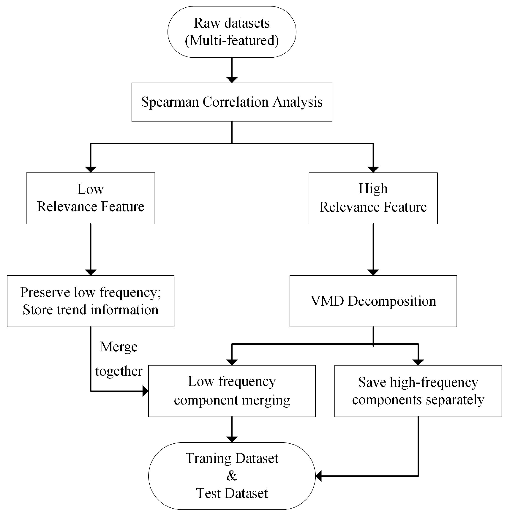
Figure 1. Flowchart of Feature Engineering Process.
Sustainability 17 09746 g001
Figure 2. Spearman correlation calculation results.
Sustainability 17 09746 g002
Figure 3. Comparison of Data Volume Before and After Feature Processing.
Sustainability 17 09746 g003
Figure 4. Spearman Correlation Results Between Processed Features and Load Values.
Sustainability 17 09746 g004
Figure 5. Comparison of Forecasting Performance Before and After Feature Processing.
Sustainability 17 09746 g005
Figure 6. Random Initialization of Population.
Sustainability 17 09746 g006
Figure 7. Tanh-Sobol Initialization of Population.
Sustainability 17 09746 g007
Figure 8. Comparison of Exploration Probability.
Sustainability 17 09746 g008
Figure 9. Comparative Curves of Exploration Probability and Step-Size Control.
Sustainability 17 09746 g009
Figure 12. Performance of Optimization Algorithms on F1(x).
Sustainability 17 09746 g012
Figure 13. Performance of Optimization Algorithms on F2(x).
Sustainability 17 09746 g013
Figure 14. Performance Comparison of IBWO Variants on F1(x).
Sustainability 17 09746 g014
Figure 18. Architecture Diagram of the Proposed Forecasting Algorithm.
Sustainability 17 09746 g018
Figure 19. Prediction Fit Curves of Baseline Models.
Sustainability 17 09746 g019
Figure 20. Performance Comparison of Baseline Prediction Models.
Sustainability 17 09746 g020
Figure 21. Performance Comparison of Models with Dilated Structures.
Sustainability 17 09746 g021
Figure 22. Evaluation Metrics of Models with Dilated Structures.
Sustainability 17 09746 g022
Figure 23. Fitness Value Convergence Curves.
Sustainability 17 09746 g023
Figure 24. Comparison of Fitting Performance of Dilated BiGRU Enhanced by Different Optimization Algorithms.
Sustainability 17 09746 g024
Figure 25. Comparison of Prediction Performance Metrics of Models Enhanced by Different Optimization Algorithms.
Sustainability 17 09746 g025
Figure 26. Robustness Evaluation of Model Fitting on Georgia Load Data.
Sustainability 17 09746 g026
Figure 27. Comparison of Prediction Performance Metrics under Robustness Evaluation.
Sustainability 17 09746 g027
Table 1. Feature Names and Descriptions in the Dataset.
Column NameDescription
nat_demandNational electricity load
T2M_tocTemperature at 2 m in Tocumen, Panama City
QV2M_tocRelative humidity at 2 m in Tocumen, Panama City
TQL_tocLiquid precipitation in Tocumen, Panama City
W2M_tocWind Speed at 2 m in Tocumen, Panama City
dayOfWeekDay of the week, starting on Saturdays
weekendWeekend binary indicator
holidayHoliday binary indicator
hourOfDayHour of the day
Table 2. Feature Names and Sample Counts in the Input Dataset for the Model.
Column NameDescriptionSample Count
nat_demandNational electricity load12,431
nat_highHigh-frequency component of nat_demand extracted via VMD12,431
T2M_highHigh-frequency component of temperature (T2M_toc) extracted via VMD12,431
hour_highHigh-frequency component of time (hourOfDay) extracted via VMD12,431
lowCombined result of all low-frequency components12,431
Table 3. Performance Comparison Before and After Feature Engineering Across Different Models.
All Features Kept After DecompositionRaw Data Input DirectlyData Processed as Proposed in This Paper
ModelRMSER2MAERMSER2MAERMSER2MAE
GRU68.59340.859751.573265.86010.870549.544261.38930.888846.3095
BiLSTM65.71280.873848.673765.62790.878648.631260.06190.891245.0527
BiGRU64.20050.881748.745662.55170.890448.349752.31610.913239.8785
Table 4. Performance of Four Optimization Algorithms on F1(x).
IBWOBWOAVOASSASO
Optimum value0.00000.00007.21460.00074.0316
Average value0.25820.834210.69774.718819.2316
Standard deviation4.44995.81638.318813.554213.7100
Table 5. Performance of Four Optimization Algorithms on F2(x).
IBWOBWOAVOASSASO
Optimum value4.64 × 10−241.18 × 10−50.63063.71 × 10−24.4151
Average
value
1.67 × 1062.61 × 1064.28 × 1069.77 × 1061.07 × 107
Standard deviation2.89 × 1073.27 × 1073.06 × 1075.83 × 1074.71 × 107
Table 6. Statistical Performance Metrics of IBWO Ablation Combinations on F1(x).
IBWOOriginal
BWO
BWO+
Tanh-Sobol
BWO+
Improved Fall
BWO+
Dynamic Levy
BWO+
Tanh-Sobol+
Improved Fall
BWO+
Tanh-Sobol+
Dynamic Levy
BWO+
Dynamic Levy+
Improved Fall
Optimum value0.00000.00000.00000.00000.00000.00000.00000.0000
Average value0.25820.83420.57580.62980.55500.59820.42640.3301
Standard deviation4.44995.81635.05605.89476.01576.28865.11614.5394
Table 7. Evaluation Metrics for Baseline Models.
ModelRMSER2MAE
ARIMA77.10890.827259.6386
RF74.08670.845357.1238
SVR71.14530.859052.6656
RNN69.72170.861354.5778
XGBoost69.36990.863652.9690
LSTM63.20300.874846.4893
GRU61.38930.888846.3095
BiLSTM60.06190.891245.0527
BiGRU52.31610.913239.8785
Table 8. Evaluation Metrics of Dilated Models.
ModelRMSER2MAE
Dilated LSTM52.97190.918040.5714
TCN50.59410.922239.0946
Dilated GRU48.96880.929738.2667
Dilated BiLSTM46.15170.939933.7720
Dilated BiGRU44.04560.946431.9781
Table 9. Comparison of the Impact of Different Optimization Strategies on Model Prediction Performance.
ModelRMSER2MAE
SO-Dilated BiGRU38.84690.953530.1231
SSA-Dilated BiGRU36.75200.963227.3250
AVOA-Dilated BiGRU34.48260.967125.3018
BWO-Dilated BiGRU27.26820.978419.5211
IBWO-Dilated BiGRU26.17060.981218.5462
Table 10. Comparison of Model Prediction Performance on an External Dataset.
ModelRMSER2MAE
BiGRU82.51580.895468.2491
TCN76.05640.903564.4329
Dilated BiGRU60.88320.942450.0802
BWO-Dilated BiGRU46.36150.966136.8688
IBWO-Dilated BiGRU38.80910.978331.0496
Table 11. Comparison of Model Performance in Prediction Accuracy, Training Time, and Memory Usage.
ModelRMSER2MAETimeMemory
Usage
ARIMA77.10890.827259.6386314.2207.1
RF74.08670.845357.1238377.1214.5
SVR71.14530.859052.6656410.7226.8
RNN69.72170.861354.5778450.6230.4
XGBoost69.36990.863652.9690540.3291.7
LSTM63.20300.874846.4893513.6240.1
GRU61.38930.888846.3095498.7233.8
BiLSTM60.06190.891245.0527554.9251.1
BiGRU52.31610.913239.8785521.7247.6
TCN50.59410.922239.0946566.8307.4
Dilated BiGRU44.04560.946431.9781589.1266.3
BWO-Dilated BiGRU27.26820.978419.5211852.7279.4
IBWO-Dilated BiGRU26.17060.981218.5462873.5286.2
Disclaimer/Publisher’s Note: The statements, opinions and data contained in all publications are solely those of the individual author(s) and contributor(s) and not of MDPI and/or the editor(s). MDPI and/or the editor(s) disclaim responsibility for any injury to people or property resulting from any ideas, methods, instructions or products referred to in the content.