Article

A Network Theory Approach to Assessing Environmental Sustainability in the Cruz Grande Region, Guerrero, Mexico

by
Luis A. Lucrecio
1,†,
Paul Bosch
2,†,
Edil D. Molina
3,*,†,
José Luis Rosas-Acevedo
1,† and
José M. Sigarreta
3,†
1
Centro de Ciencias de Desarrollo Regional (CCDR), Universidad Autónoma de Guerrero, Privada del Laurel No. 13, Col. El Roble, Acapulco de Juárez 39640, Guerrero, Mexico
2
Facultad de Ingeniería, Universidad del Desarrollo, Ave. La Plaza 680, San Carlos de Apoquindo, Las Condes, Santiago 7610658, Chile
3
Facultad de Matemáticas, Universidad Autónoma de Guerrero, Carlos E. Adame No. 54, Col. Garita, Acapulco de Juárez 39650, Guerrero, Mexico
*
Author to whom correspondence should be addressed.
These authors contributed equally to this work.
Sustainability 2025, 17(21), 9731; https://doi.org/10.3390/su17219731
Submission received: 25 July 2025 / Revised: 14 October 2025 / Accepted: 29 October 2025 / Published: 31 October 2025

Abstract

Traditional composite indicators for the study of sustainability often obscure the complex network of relationships among individual indicators, functioning as black boxes that fail to diagnose the underlying structural and functional weaknesses of the system. The objective of this research is to develop and apply a complementary approach grounded in network theory to diagnose and evaluate the structural and functional cohesion of environmental indicator systems. We developed a study that combines the Principal Component Analysis (PCA) method with network theory to comprehensively analyze the indicator system. The core of this contribution is the development of the M o ( G ) index, designed to quantify the structural–functional cohesion of an indicator network. This approach is applied to an environmental dataset of 19 indicators for Cruz Grande, Guerrero, Mexico (2010–2023). The results reveal that although the indicator network is relatively dense ( d = 0.6199 ), its structural–functional cohesion is low ( M o ( G ) = 520.68 ), placing the region in the Fair category. This result provides an explanation for the sustained decline of the system, as shown by the PCA-based Regional Environmental Sustainability Index. We conclude that this approach is a complementary tool for diagnosing and evaluating environmental systems, enabling the detection of vulnerabilities that remain invisible to conventional aggregation methods.

1. Introduction

Sustainability, elevated to a central paradigm in decision-making by the Brundtland Report [1], has become a key guiding concept. In that report, sustainability was defined as the ability to meet the needs of the present without compromising the ability of future generations to meet their own. Far from being a purely environmental concern, sustainability is intrinsically multidimensional, seeking a dynamic and equitable balance among environmental integrity, social equity, and economic viability [2]. Achieving this balance requires a deep understanding of the interdependencies between human and natural systems, as well as a commitment to intergenerational equity.
However, this normative ideal contrasts sharply with the current global socio-environmental crisis, characterized by systemic overexploitation of natural resources that exceeds the regenerative capacity of ecosystems [3]. The persistent gap between sustainability as a guiding principle and the degradation observed in practice has created an urgent need for tools capable of operationalizing the concept of sustainable development in ways that are both concrete and context-sensitive.
In response, academics, institutions, and governments have turned to the development of sustainability indicators: metrics designed to translate the complexity of socio-environmental systems into interpretable, comparable, and actionable information. These metrics can take the form of individual indicators, which track specific variables such as carbon emissions, land use, or water consumption, and are often valued for their clarity and precision. However, individual indicators often fail to capture the complex web of relationships that defines the systemic and multidimensional nature of sustainability, especially when interactions and trade-offs between variables are significant [4].
To address these limitations, composite indicators (indices) have been proposed as integrative tools that synthesize multiple variables through processes of normalization, weighting, and aggregation. These aim to represent sustainability more holistically, enhancing both communication and comparability across contexts [5]. Prominent early examples include the Human Development Index (HDI) [6], which focuses on health, education, and income. This was followed by indicators that incorporate environmental dimensions, such as the Environmental Sustainability Index (ESI) [7] and the Environmental Performance Index (EPI) [8]. More recent proposals, like the Sustainable Development Index (SDI) [9] and the Sustainable Human Development Index (SHDI) [10], attempt to penalize ecological overshoot explicitly.
Despite their wide adoption and conceptual evolution, composite indicators are often criticized for relying on compensatory aggregation methods (e.g., arithmetic or geometric means), which can obscure internal imbalances between dimensions and trade-offs that are crucial for sustainability assessments [5]. Additionally, these indicators frequently treat component variables as independent, thereby ignoring the relational structure and interdependencies that define complex socio-environmental systems. Such methodological shortcomings are particularly problematic in territories with limited data availability, institutional fragility, and high levels of environmental and social vulnerability.
These limitations become acutely relevant in rural and marginalized regions, where decision-making is often determined by top-down governance structures that neglect local perspectives and capacities. In the La Sabana-Laguna de Tres Palos river sub-basin, located in Acapulco, Guerrero, Mexico, for example, historically vertical and politically driven approaches have repeatedly undermined integrated environmental management and the construction of long-term strategies [11]. This broader pattern of institutional fragility and ineffective planning is acutely evident in rural localities such as Cruz Grande, Guerrero, Mexico, characterized by limited infrastructure, high levels of marginalization, and a predominantly agricultural economy. In these contexts, the absence of scientifically based and territorially relevant diagnostic tools severely hinders the ability of local actors to evaluate, design, or assess sustainability initiatives. As a result, ineffective planning practices persist, reinforcing the very power asymmetries and institutional deficiencies they seek to overcome.
This study addresses the aforementioned diagnostic gap by proposing and applying a complementary approach based on network theory to diagnose and evaluate environmental sustainability. The objective is to overcome conventional aggregation methods by combining a temporal performance analysis with an evaluation of the structural–functional cohesion of the system.
The proposed framework combines principal component analysis (PCA) with network theory to comprehensively analyze the indicator system. On the one hand, PCA is used to calculate the Regional Environmental Sustainability Index ( R E S I ), a composite indicator adapted to the Mexican rural context [12]. The R E S I provides a benchmark metric that is used to empirically validate the results of our network study. On the other hand, the central contribution of the study is the M o ( G ) index, designed to quantify the structural–functional cohesion of the indicator system. This diagnosis is complemented by traditional graph theory metrics, such as density, centrality, modularity, and the assortativity coefficient, which allow for a more in-depth analysis of the network structure. To demonstrate its usefulness, this approach is applied to the case study of Cruz Grande, Guerrero, using a set of environmental data of 19 indicators grouped into three thematic categories: water management, land use and solid waste, and general environmental metrics.
By integrating PCA with a network theory-based approach, and particularly by introducing the M o ( G ) index, this study offers a complementary tool for diagnosing environmental sustainability. This approach considers both temporal dynamics and systemic structure, allowing it to uncover vulnerabilities that are not apparent to conventional aggregation methods. The methodology is especially well-suited for rural environments like Cruz Grande, where traditional data limitations require more creative and structurally sensitive approaches. This work does not directly address the broader political or institutional challenges of sustainability governance. However, it does provide a basis for more informed, territorially grounded, and analytically robust planning processes. In this regard, a software tool designed to assist in decision-making is proposed.

2. Theoretical Background

Network theory has become a fundamental framework in sustainability science, offering a language capable of capturing the complexity of socio-ecological systems. This approach is described as a relational shift in recent literature [13,14]. It moves the focus from the isolated properties of species, actors, or institutions to the interactions that shape a system’s resilience and transformative capacity. In this sense, sustainability is conceived as an emergent property of network configurations rather than a fixed state that can be achieved in a linear manner [15].
In ecology, the pioneering work of Bascompte and Jordano showed that mutualistic networks exhibit non-random patterns, such as nestedness and modularity, which favor stability and species coexistence [16,17]. These contributions consolidated the network approach for studying biodiversity and resilience. They demonstrated that the architecture of connections conditions a community’s persistence and its response to disturbances [18]. Within this field, recent studies have applied network metrics to assess the resilience of forests to global threats, integrating network properties with functional traits to predict ecosystem response [19].
In research on socio-ecological systems, network theory has provided tools for understanding the governance of common goods and patterns of cooperation. Levin conceptualized ecosystems as complex adaptive systems characterized by nonlinearity and self-organization [20], while Ostrom proposed a multilevel framework for analyzing the sustainability of shared resources [21]. Subsequently, Gonzalès and Parrott [22] directly applied network metrics to assess the resilience of socio-ecological systems, opening a field of research that has grown steadily over the last decade.
The consolidation of this approach is reflected in the systematic review by Sayles et al. [23], which synthesizes the development of socio-ecological network (SEN) analysis. This work highlights that while SENs have successfully integrated social and ecological domains, significant gaps remain in linking structural patterns to environmental outcomes. The review identifies a strong reliance on traditional metrics and raises the need to move toward dynamic, multilayer, and longitudinal networks. These conclusions align with foundational contributions from authors like Janssen et al. [24] and Norberg and Cumming [25], who had already emphasized a relational framework for studying resilience. They are also consistent with later works showing how certain network configurations facilitate cooperation and the provision of ecosystem services [26,27,28]. More recent research has explored the use of higher-order analysis, such as simplicial topology, to capture complex interactions in socio-ecological networks, revealing collaborative structures beyond simple peer-to-peer interactions [29].
The empirical applications of network theory in sustainability are diverse. In environmental governance, Bodin and Crona [30] analyzed how social networks influence the co-management of natural resources, and more recent studies have employed dynamic models to assess the resilience of forest systems [31]. In rural coastal communities, Aguilar-Becerra et al. [32] showed how combining social network analysis with path-dependent trajectories explains the evolution of tourism and its sustainability. Furthermore, in applied ecology, Pineda-Pineda et al. [33] used bipartite networks to assess water quality.
Other areas of application include industry and international politics. Larrea-Gallegos et al. [34] conducted a comprehensive review to propose an agent-based approach for simulating sustainable and resilient supply networks. Kim and Allenby [35] developed sustainability network theory (SNT) as a framework for modeling energy, material, and information flows in complex industrial systems. In the policy domain, Nilsson et al. [36] showed that the Sustainable Development Goals (SDGs) can be mapped as a network of interactions. This mapping reveals synergies and trade-offs that require coordinated management. Benhar et al. [37] extended this approach using complex network theory, applying small-world and many-body system models to interdisciplinary cooperation around the SDGs. Finally, Dragicevic [38] proposed a concentric framework for sustainability assessment, using a hypergraph approach to study the resilience and connectivity of a socio-ecological system.
In parallel, conceptual approaches such as actor–network theory have emerged, emphasizing the symmetry between human and non-human actors in socio-technical transition processes. Aka [39] reviews how this perspective has been applied in sustainability research, particularly in urban governance and industrial processes. Likewise, studies by authors such as Liu et al. [40] have shown the importance of global teleconnections. They highlight how flows of information, capital, and resources generate transnational networks with crucial implications for sustainability.
This bibliographic analysis shows that network theory has established itself not only as a cross-cutting field of research but also as a bridge between previously isolated disciplines. Barabási [41] anticipated this transition, noting that networks would dominate the new century to a degree that is difficult to imagine and that network thinking would invade most fields of human activity. This vision reinforces the need for a systemic approach that allows us to recognize the hidden interactions between social, economic, and environmental dimensions, thereby contributing to the design of more integrated policies and strategies.
In this context, the novelty of our work lies in applying network theory as an analytical tool, going beyond its purely conceptual or descriptive use. For the study, we combined widely used metrics, such as centralities, with less explored properties such as nodal energy and structural relationships, which allowed us to evaluate the structural–functional cohesion of the environmental indicator system. This proposal broadens the field of application of network theory. While previous research focused only on the topological and structural properties of such networks, our analysis directly addresses the interrelationship between environmental indicators and their internal vulnerabilities. This positions our work as an original contribution that favors the evaluation of complex systems associated with sustainability, with the potential to be replicated and adapted in other territorial contexts.

3. Methodology

3.1. Analytical Techniques

The methodological approach of this research is structured around two key techniques: Principal Component Analysis and Network Theory. The foundations of both techniques are detailed below.

3.1.1. Principal Component Analysis (PCA)

Principal Component Analysis (PCA) is a multivariate statistical technique widely used in sustainability assessment to reduce the dimensionality of complex datasets and identify their latent structures [42,43]. Instead of examining numerous correlated indicators in isolation, PCA transforms them into a smaller set of uncorrelated variables known as principal components, each capturing the maximum possible variance from the original data [44].
PCA is a well-established tool in sustainability science for its effectiveness in synthesizing complex datasets. For instance, it has been used to construct composite indicators for assessing the sustainability of manufacturing companies [45] and to integrate diverse social and infrastructural variables in urban sustainability assessments [46].
Mathematically, PCA transforms the original data matrix X R n × p —where n is the number of observations and p the number of indicators—into a set of uncorrelated variables Z 1 ,   Z 2 ,   ,   Z p . Each principal component is a linear combination of the standardized indicators:
Z k = ω k 1 X 1 + ω k 2 X 2 + + ω k p X p , for   k = 1 , , p ,
where ω k j for j = 1 , , p are the loadings (or weights) assigned to each indicator X j in the construction of the k-th component Z k . These weights are chosen so that the first component Z 1 captures the maximum possible variance. Each subsequent component then captures the highest remaining variance while being uncorrelated with the previous ones.
To apply PCA effectively, the following steps are typically followed:
1.
Assessment of Data Suitability: The data’s fitness for factor analysis is verified using the Kaiser-Meyer-Olkin (KMO) measure and Bartlett’s test of sphericity [47].
2.
Standardization of the data: Each indicator is transformed to have a mean of zero and a standard deviation of one:
X j = X j X ¯ j σ j ,
where X ¯ j is the mean and σ j the standard deviation of the indicator X j . This step ensures comparability between variables with different units.
3.
Computation of the correlation matrix R: Since the variables are standardized, their interdependencies are summarized in the matrix R, where each entry r i j represents the Pearson correlation between indicators X i and X j .
4.
Extraction of components: The principal components correspond to the eigenvectors of the matrix R, and the amount of variance each one explains is given by the associated eigenvalue λ s divided by total variance in the dataset,
Variance   explained   by   the   s - th   component = λ s k = 1 p λ k .
5.
Selection of components: The decision on how many components to retain is guided by established statistical criteria, such as Horn’s parallel analysis, Velicer’s minimum average partial (MAP) test, and the visual inspection of the scree-plot “elbow” [42,48,49,50]. However, in the specific context of constructing composite indicators, interpretability is paramount.For this reason, the standard procedure is to use only the first principal component ( Z 1 ). This is done provided provided it explains a substantial portion of the total variance (above 0.50). This practice avoids the informational and sign-inconsistency issues that secondary components can introduce, ensuring the final index has a clear and unambiguous meaning [5,51,52,53].
6.
Calculation of component scores: Each observation receives a score on each retained component. These scores can be used to build composite indicators or to compare performance across regions.
In this study, we define a temporal index, denoted as RESI. The index is computed by projecting standardized indicator values onto the first principal component,
RESI = i = 1 p ω 1 i z t i ,
where z t i is the standardized value of indicator i at time t, and ω i is its corresponding loading. The resulting time series RESI summarizes the dominant trend across indicators, enabling consistent temporal evaluation.
This formulation follows the same methodological framework as the ISAM index developed for southeastern Mexico [12], which also relies on principal component analysis to aggregate environmental indicators. The ISAM provides a static comparison across municipalities. In contrast, our version introduces a temporal perspective that allows for the identification of structural shifts and long-term trends within a single locality.
By extending the PCA-based approach to the temporal domain, the proposed index enhances the interpretative capacity of sustainability assessments. It serves as both a benchmarking tool aligned with national metrics and a diagnostic mechanism tailored to local dynamics.
It is important to acknowledge the methodological challenges inherent to this technique. A primary concern is its reliance on linear assumptions, which may fail to capture the complex, non-linear dynamics often present in socio-ecological systems [44]. The interpretability of the resulting components can also be difficult, as these mathematical constructs may not align neatly with established conceptual frameworks of sustainability. Several studies have noted these challenges, particularly in aligning the statistical outputs with policy-relevant dimensions [5,54]. Furthermore, its compensatory nature can mask critical trade-offs between individual indicators [4].

3.1.2. Network Theory

A network is formally defined as a collection of nodes (also called vertices) connected by links (or edges) [41,55]. The structure of the network is encoded in its adjacency matrix A = [ a i j ] , where
a i j = 1 , if   node   i   is   linked   to   node   j , 0 , otherwise .
We focus on undirected networks, where links represent mutual relationships and the adjacency matrix A is symmetric. Several structural concepts from network theory play a central role in this study. The degree of a node i, denoted d i = j a i j , corresponds to the number of direct links it maintains. This quantity indicates how interconnected a node is within the system.
A fundamental descriptor of the overall network structure is its density, defined as the ratio between the number of existing links m and the maximum number of possible links. For a network with n nodes, the density is computed as
d = 2 m n ( n 1 ) .
High-density networks suggest a system of tightly interrelated components, while sparse networks may reflect compartmentalized or weakly coordinated subsystems.
The concept of a path captures the notion of connectivity between two nodes. A path is a sequence of nodes v 1 ,   v 2 ,   ,   v k such that each consecutive pair is directly linked. The distance between two nodes u and v, denoted d ( u , v ) , is the length of the shortest path connecting them. A network is said to be connected if there exists at least one path between every pair of nodes. This property guarantees that the system forms a single coherent structure, enabling the calculation of global measures such as spectral or centrality mesures. In contrast, disconnected networks may yield misleading or fragmented diagnostics.
The clustering coefficient quantifies the extent to which the neighbors of a given node are themselves interconnected, offering insight into local cohesion. Complementarily, centrality measures identify nodes of structural significance. These include:
  • Degree centrality, computed as
    C D ( u ) = d u n 1 ,
    measures the proportion of nodes directly connected to u.
  • Closeness centrality, given by
    C C ( u ) = n 1 v u d ( u , v ) ,
    reflects the proximity of a node to all others.
  • Betweenness centrality, defined as
    C B ( u ) = s u t σ s t ( u ) σ s t ,
    quantifies how frequently node u lies on shortest paths between other nodes. Here, σ s t is the number of shortest paths from s to t, and σ s t ( u ) the number passing through u.
  • Eigenvector centrality assigns higher scores to nodes connected to other central nodes. It is calculated as
    C E ( u ) = x 1 ( u ) ,
    where x 1 ( u ) is the u-th component of the principal eigenvector of the adjacency matrix.
In addition to topological descriptors, spectral properties derived from the eigenvalues of the adjacency matrix provide global information about the organization, robustness, and modularity of the system. These measures form the basis for constructing more refined structural indices, as explored later in this work.
Certain archetypal structures in network theory serve as useful references for interpreting empirical networks. A tree is a connected network that contains no cycles, meaning there is exactly one unique path between any pair of nodes. Among trees, two canonical forms are of particular interest. A path network arranges the nodes in a linear sequence, resulting in maximal average distance and minimal centralization (see Figure 1). In contrast, a star network consists of a central node connected to all others, which are not connected among themselves. This configuration exhibits extreme centralization and minimal average distance. Both represent limiting cases of connectivity and centrality within minimal link structures.
At the opposite end of the spectrum lies the complete network, where every node is directly linked to every other. Such a network with n nodes has the maximum possible number of links, m = n ( n 1 ) 2 , and achieves a density of 1. In the context of sustainability analysis, a complete network would suggest total interdependence among all indicators. While this situation is rare in practice, it is theoretically useful as a benchmark for evaluating empirical density and redundancy.
This collection of theoretical constructs and structural metrics forms the foundation for our network-based sustainability analysis.

3.2. The M o ( G ) Index

In order to quantify the structural–functional cohesion of sustainability networks, we introduce a novel index, denoted as M o ( G ) . This index builds upon the concept of node energy formulated by Arizmendi et al. [56]. It aims to synthesize both the local spectral prominence of each node and the topological configuration of the network as a whole.
Given an undirected, simple, and connected network G = ( V , E ) with n nodes and adjacency matrix A = [ a i j ] . The spectral decomposition of A yields a set of real eigenvalues λ 1 ,   λ 2 ,   ,   λ n and corresponding orthonormal eigenvectors ϕ 1 ,   ϕ 2 ,   ,   ϕ n .
The energy of a node u V is defined in [56] as
ε u = j = 1 n | λ j | · ( ϕ j ( u ) ) 2 ,
where ϕ j ( u ) denotes the u-th component of eigenvector ϕ j . This value captures the extent to which the node is embedded in the network’s dominant modes of interaction, reflecting both its position and role within the overall system.
Using this localized energy, we define the M o ( G ) index as a sum over all unordered pair of nodes, formally:
M o ( G ) = u v ε u + ε v d ( u , v ) ,
where d ( u , v ) denotes the shortest-path distance between nodes u and v. This formulation aggregates the pairwise energy, assigning more weight to proximal node pairs, and penalizing distant connections. The inclusion of d ( u , v ) ensures that the index reflects not only the spectral prominence of nodes, but also their structural accessibility within the network.
Conceptually, M o ( G ) captures a trade-off between energy and distance, configurations where high-energy nodes are centrally connected yield higher index values, indicating a cohesive and potentially resilient structure. In contrast, fragmented or loosely connected systems result in lower M o ( G ) scores, revealing a loss of integrative capacity.
For a detailed example of the M o ( G ) index computation, the reader is referred to Appendix A.
While the definition of M o ( G ) is based on pairwise interactions between all nodes, it can be elegantly reformulated to reveal the individual contribution of each node. The following result shows that the M o ( G ) index is equivalent to a weighted sum of the node energies, this provides a powerful node-centric perspective on the index. For the sake of clarity and brevity, the detailed proofs for all propositions in this section are presented in Appendix B.
Proposition 1.
Let G be a connected graph with set of nodes V ( G ) . Then,
M o ( G ) = v V ( G ) ε v u v 1 d ( u , v ) .
We now analyze several theoretical properties of the proposed index M o ( G ) . By analyzing the behavior of the index under general constraints on node degrees and network distances, we derive a set of upper and lower bounds. These results offer interpretative insight into the index’s formulation and establish benchmark inequalities useful for comparative analysis across different classes of networks.
The concept of network energy was originally introduced by Gutman in the context of chemical network theory [57]. It quantifies the total oscillatory behavior of a network’s structure through the eigenvalues of its adjacency matrix. For a network G the total energy is defined as
E ( G ) = i = 1 n | λ i | .
This quantity captures the global spectral content of the network and has been widely used to assess structural complexity and symmetry.
In the context of the index M o ( G ) it is natural to investigate how the total energy E ( G ) constrains the overall magnitude of M o ( G ) . The following proposition establishes upper and lower bounds for M o ( G ) in terms of E ( G ) and the network diameter.
Proposition 2.
Let G be a connected network with n nodes, then
n 1 diam ( G ) E ( G ) M o ( G ) ( n 1 ) E ( G ) .
For any connected network G with maximum degree Δ 1 , the node energy ε v of a node v is bounded as follows (see [56], Proposition 3.2 and Theorem 3.6)
d v Δ ε v d v .
This result allow us to prove the following.
Proposition 3.
Let G be a connected network with maximum degree Δ 1 . Then,
1 Δ u v d u + d v d ( u , v ) M o ( G ) u v d u + d v d ( u , v ) .
The following result establishes bounds for the index M o ( G ) in terms of the well-known topological index M 1 a ( G ) named generalized first Zagreb index, evaluated at the exponent a = 3 2 . This index was defined in [58] as
M 1 a ( G ) = u V ( G ) d u a = u v E ( G ) d u a 1 + d v a 1 .
This classical degree-based index reflects the local contribution of nodes degrees to the structure of the network.
Proposition 4.
Let G be a connected network with n nodes, m links, maximum degree Δ, and minimum degree δ. Then
1 Δ M 1 3 / 2 ( G ) + 2 δ diam ( G ) n 2 m M o ( G ) M 1 3 / 2 ( G ) + Δ n 2 m .
A well-known distance-based topological invariant is the Harary index, denoted H ( G ) . This index is defined as
H ( G ) = u v 1 d ( u , v ) .
Originally proposed in [59] as a measure of molecular compactness, the Harary index captures inverse distance efficiency. It is particularly useful in quantifying the extent of global communication or proximity within a network.
Proposition 5.
Let G be a connected network with maximum degree Δ and minimum degree δ. Then,
2 δ Δ H ( G ) M o ( G ) 2 Δ H ( G ) .
We now derive bounds for the index M o ( G ) in terms of the classical Wiener index W ( G ) , defined as
W ( G ) = u v d ( u , v ) .
This topological index was originally introduced by Harold Wiener in 1947 [60] to model the boiling points of paraffin compounds. It has since become one of the most widely used descriptors in chemical graph theory.
Proposition 6.
Let G be a connected network with n nodes, maximum degree Δ and minimum degree δ. Then,
δ n 2 ( n 1 ) 2 2 Δ W ( G ) M o ( G ) Δ n 2 ( n 1 ) 2 ( D + 1 ) 2 8 D W ( G ) ,
where D = diam ( G ) .

3.3. Study Area and Data Collection

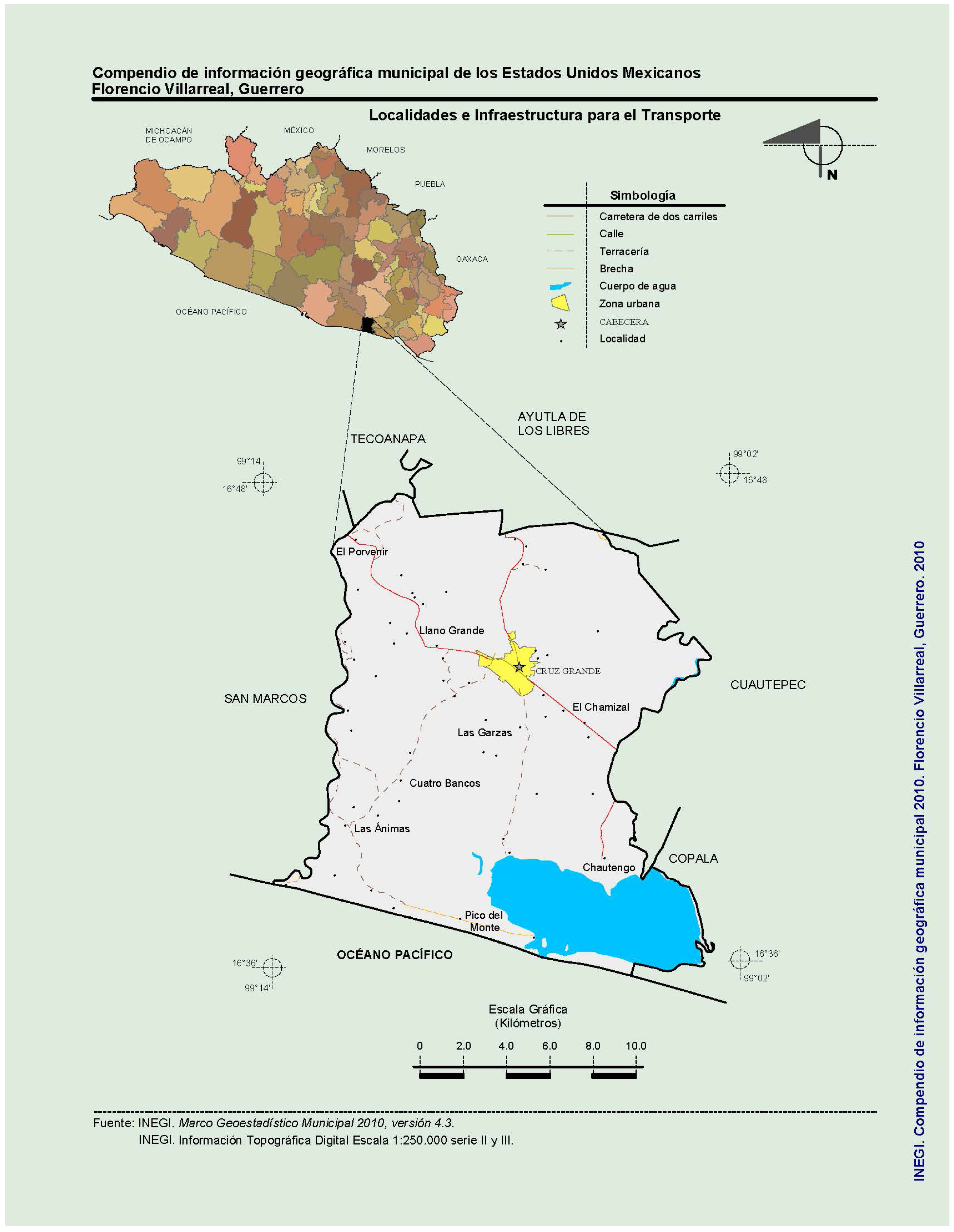
The municipality of Florencio Villarreal (Figure 2) is located in the southern region of the state of Guerrero, Mexico, along the Costa Chica area and bordering the Pacific Ocean. Its municipal seat is the town of Cruz Grande, situated at approximately 99°07′24″ west longitude and 16°43′26″ north latitude, slightly northwest of the Equator. The municipality is bounded to the north by Ayutla de los Libres and Tecoanapa, to the east by Cuautepec and Copala, to the west by San Marcos, and to the south by the Pacific Ocean. The average elevation is approximately 30 m above sea level, and its total surface area is 372.90 km2, accounting for 0.58% of the state’s total area, according to the Municipal Development Plan [61].
To construct the sustainability assessment, a time-series dataset was compiled for 19 environmental indicators covering the period 2010–2023. The data were sourced from official national databases, ensuring consistency and reliability. Primary sources included the Agrifood and Fisheries Information Consultation System [63], the Population and Housing Censuses [64,65,66], the Sustainable Development Goals Indicators platform [67], and the National Commission for the Knowledge and Use of Biodiversity [68].
The selection of these indicators was based on their interpretability, variability, and relevance to the local context. To provide a clear conceptual structure, they were organized into three thematic categories:
  • Water management, including metrics on access to piped water, well density, and wastewater treatment coverage.
  • Land use and solid waste, with indicators such as urban encroachment near water bodies, waste collection efficiency, and land use balance.
  • General environmental metrics, covering aspects like CO2 emissions per capita, renewable energy consumption, and forest cover.
The selection of these 19 indicators was further validated against established international and national frameworks, including the Environmental Performance Index (EPI), the Ecological Footprint Index (EFI), the ISAM index, and the SDGs. As shown in Table 1, 89% of the indicators (17 out of 19) have precedents in these recognized systems, which enhances the scientific robustness and comparability of our study.
The indicator for Forest and jungle coverage change ( I 19 ) was quantified by analyzing historical satellite imagery from the Google Earth™ platform, following a visual comparison method similar to that of Avilés-Ramírez et al. [69]. Polygons representing areas with loss of vegetation cover were manually digitized for different years. The surface area of these polygons, obtained from official cartography [66], allowed for the calculation of the annual and cumulative deforestation rate.
The indicator for Environmental impact of agricultural activities ( I 1 ) was estimated by quantifying four types of pollutants based on annual production records from SIACON [63]. Applying the fundamental estimation technique proposed by the FAO [70] and using emission factors from other international and national bodies [71,72,73,74], we calculated the annual generation of greenhouse gases, solid waste, agrochemical use and water/soil contamination. Each of these four observed values was then compared against a permissible or optimal threshold derived from the literature to express its impact as a percentage. The final value for the main indicator ( I 1 ) was determined by averaging these four individual impact percentages.
Notably, the estimation methods for indicators I1 and I19 are susceptible to introducing subjective bias. This is particularly relevant for I19, which was derived from a visual analysis of satellite images.
Furthermore, two innovative indicators were used to capture local water management realities often missed by standard composite indicators. Number of private wells ( I 7 ) was included to account for unofficial water extraction, a critical factor in aquifer overexploitation that remains largely invisible in official statistics [75]. Similarly, Public water service wells ( I 16 ) was designed to move beyond official information and assess the physical availability of public infrastructure. This address the gap between reported access and effective, equitable service for all households [76,77].

3.4. Data Validation and Preparation

Recognizing the importance of valid input data, this study, while rooted in official national and international databases, acknowledges their potential limitations in terms of representativeness and timeliness. To address this, a three-tiered complementary validation strategy was implemented. First, a direct institutional relationship between the Universidad Autónoma de Guerrero and the government of Cruz Grande allowed for the corroboration of official data with local administrative records and programs. Second, the authors’ more than ten years of personal fieldwork experience in the locality provided firsthand knowledge to contrast the indicators with observed territorial dynamics. Third, results from previously published electronic surveys of local inhabitants were integrated [78], providing empirical support for social and perceptual indicators. Periodic meetings with residents and collaborating researchers further enabled the triangulation of findings against independent evidence [79].
This multi-level approach was quantitatively reinforced. A prior study [78] allowed for the in-situ corroboration of 47% of the individual indicators ( I 3 ,   I 4 ,   I 5 ,   I 6 ,   I 7 ,   I 10 ,   I 15 ,   I 16 , and I 17 ). For the remaining indicators, a statistical analysis showed coefficient of variation (CV) values below 15%. This threshold is interpreted as low dispersion, providing evidence of adequate consistency and reliability in the data, in line with widely accepted criteria in environmental and experimental sciences [80,81].
Following this comprehensive validation process, the complete dataset—a matrix of 19 indicators over 14 years (2010–2023)—was prepared for analysis. The entire matrix was standardized using the z-score transformation (Equation (2)) to ensure all indicators were on a comparable scale. From this standardized data, the Pearson correlation matrix (R) was computed, which served as the common input for both the temporal and structural analyses. Together, these validation and preparation steps reduce the uncertainty associated with using only official data and ensure that the results reflect not only data availability but also the interpretive richness derived from the interaction between academia, local government, and the community.
Following this comprehensive validation process, the complete dataset—a matrix of 19 indicators over 14 years (2010–2023)—was prepared for analysis. Each indicator was standardized across the whole temporal series using the z-score transformation (Equation (2)). For every variable, its own mean and standard deviation were computed over the full 2010–2023 period, ensuring that all yearly observations of that variable share a common reference benchmark. From this standardized data, the Pearson correlation matrix (R) was computed as the common input for both the temporal and structural analyses.
This choice of fixed, indicator-specific normalization enhances comparability across years but may attenuate changes in the overall distribution through time. Such trade-offs between fixed and time-varying goalposts are a well-known challenge in longitudinal composite indicators [82,83], and we interpret temporal trends in light of this limitation.

3.5. Calculation of the Regional Environmental Sustainability Index

To ensure the robustness and validity of the analysis, several key statistical assumptions and procedures were addressed. First, the suitability of the data for PCA was confirmed using two diagnostic tests. The Kaiser-Meyer-Olkin (KMO) measure of sampling adequacy was calculated to assess the proportion of common variance among the indicators, with an acceptability threshold set at KMO > 0.60, consistent with methodological recommendations [84,85]. Additionally, Bartlett’s test of sphericity was performed to verify that the correlation matrix was not an identity matrix, requiring a statistically significant result ( p < 0.05 ) to proceed. The assumption of linearity was evaluated by comparing the Pearson (r) and Spearman ( ρ ) correlation matrices; pairs of indicators with a notable divergence ( | | ρ | | r | | > 0.2 ) were subjected to detailed visual inspection using scatter plots. The normality assumption was assessed with the Shapiro–Wilk test, and homoscedasticity was considered addressed by the inherent standardization of the data when using a correlation matrix. Finally, to evaluate the stability of the first principal component ( Z 1 ), a 5-fold cross-validation procedure was implemented. The dataset (n = 14 years) was randomly split into five subsets, and Z 1 was re-calculated five times. The stability of the component was confirmed by examining the consistency of the explained variance, the similarity of the loading vectors (using cosine similarity), and the coherence of variable importance rankings (measured with Spearman’s correlation on the absolute values of the loadings) across the folds [84].
Following these validation procedures, the RESI was calculated as defined in Section 3.1.1 using Equation (4). The resulting RESI time series was normalized (to mean 0, variance 1) and classified into six qualitative sustainability levels based on standard deviation intervals, as detailed in Table 2.

3.6. Network Construction and Structural Analysis

In parallel, to explore the systemic structure of the indicators, a network was constructed from the same correlation matrix R. In this network, each of the 19 indicators is represented as a node. An undirected link is established between two nodes if the absolute value of their Pearson correlation, | r i j | , exceeds a specific threshold, τ . The value of τ is methodologically determined by identifying the highest possible threshold that ensures the resulting network remains fully connected. This approach preserves the core relational structure while filtering out weaker, potentially noisy correlations.
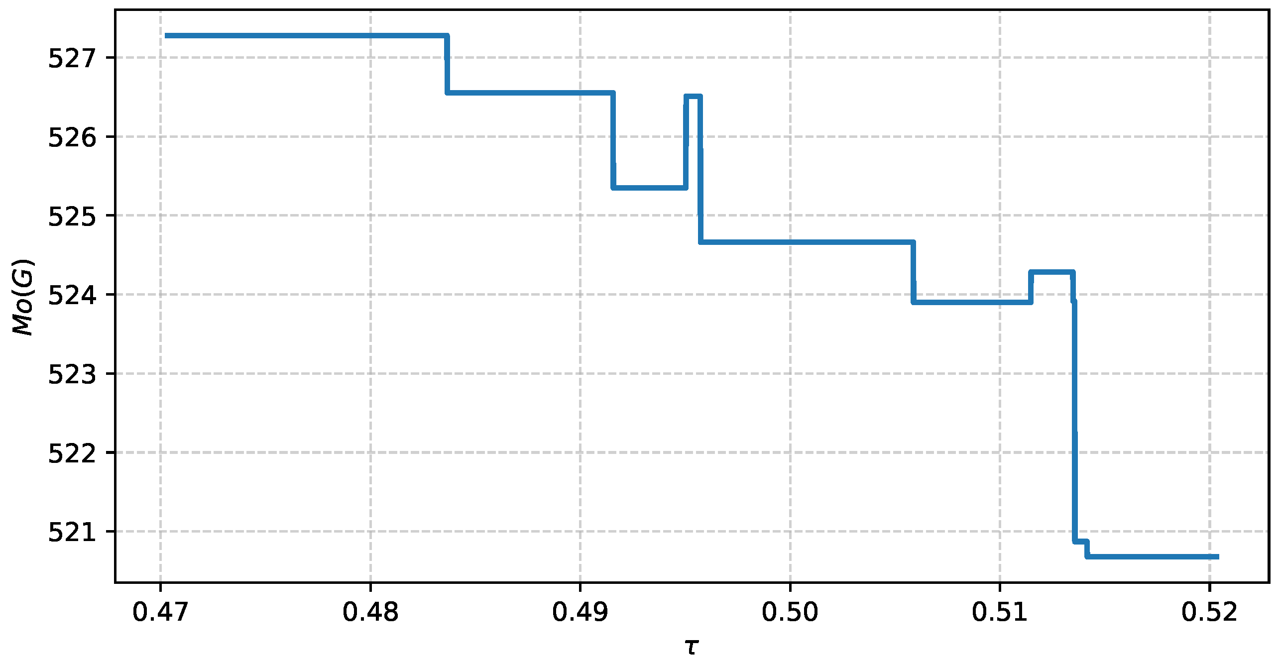
Once the network’s adjacency matrix (A) is established, the structural–functional cohesion index, M o ( G ) , is calculated as defined in Equation (11). To ensure the result is not an artifact of the specific correlation threshold ( τ ) selected, a sensitivity analysis is performed. This involves re-calculating the M o ( G ) index across the predefined interval [ τ 0.05 ,   τ ) to verify the stability of the structural diagnosis.
To provide a comprehensive characterization of the network’s topology, a suite of additional metrics will be computed. These include node-level centrality measures (degree, closeness, betweenness, eigenvector), local and global clustering coefficients, and global network properties such as diameter, average path length, and modularity, as described in Section 3.1.2.
All procedures were implemented in Python using the libraries NumPy, pandas, and NetworkX, with the aid of standard graph traversal and linear algebra routines.

3.7. Computational Study

To investigate how the magnitude of the M o ( G ) index responds to varying levels of structural complexity, we performed a computational study on an ensemble of random connected networks. The simulation was designed to assess the sensitivity, saturation, and variability of the index across the full connectivity spectrum, thereby providing a robust reference framework for interpreting empirical values.
The simulations were conducted on undirected simple networks with n = 19 nodes, corresponding to the number of environmental indicators under consideration. The network density, d, was systematically varied in the range [ 2 n , 1 ] , where the lower bound ensures the possibility of connectivity. This range was discretized with a step of Δ d = 0.025 , and for each density level, a total of 10 8 random connected networks were generated and sampled.
To guarantee connectivity, each network was generated by first constructing a random spanning tree and then adding the remaining links uniformly at random until the target density was achieved. This procedure ensures that the sample space includes only connected topologies.
For each generated network, the index M o ( G ) was computed according to its definition in Equation (11). Node energy values, ε u , were obtained following the spectral method proposed by Arizmendi et al. [56] and implemented according to the computational guidelines outlined by Gutman and Furtula [86]. Eigenvalues and eigenvectors were computed using the LAPACK subroutine DSYEV, and shortest-path distances, d ( u , v ) , were computed using a breadth-first search algorithm.
For each density level, summary statistics of M o ( G ) (mean, standard deviation, minimum, and maximum) were recorded across the ensemble of sampled networks. To enhance computational performance, simulations were executed in parallel using OpenMP. All outputs were stored in a CSV file for subsequent analysis.
4. Results

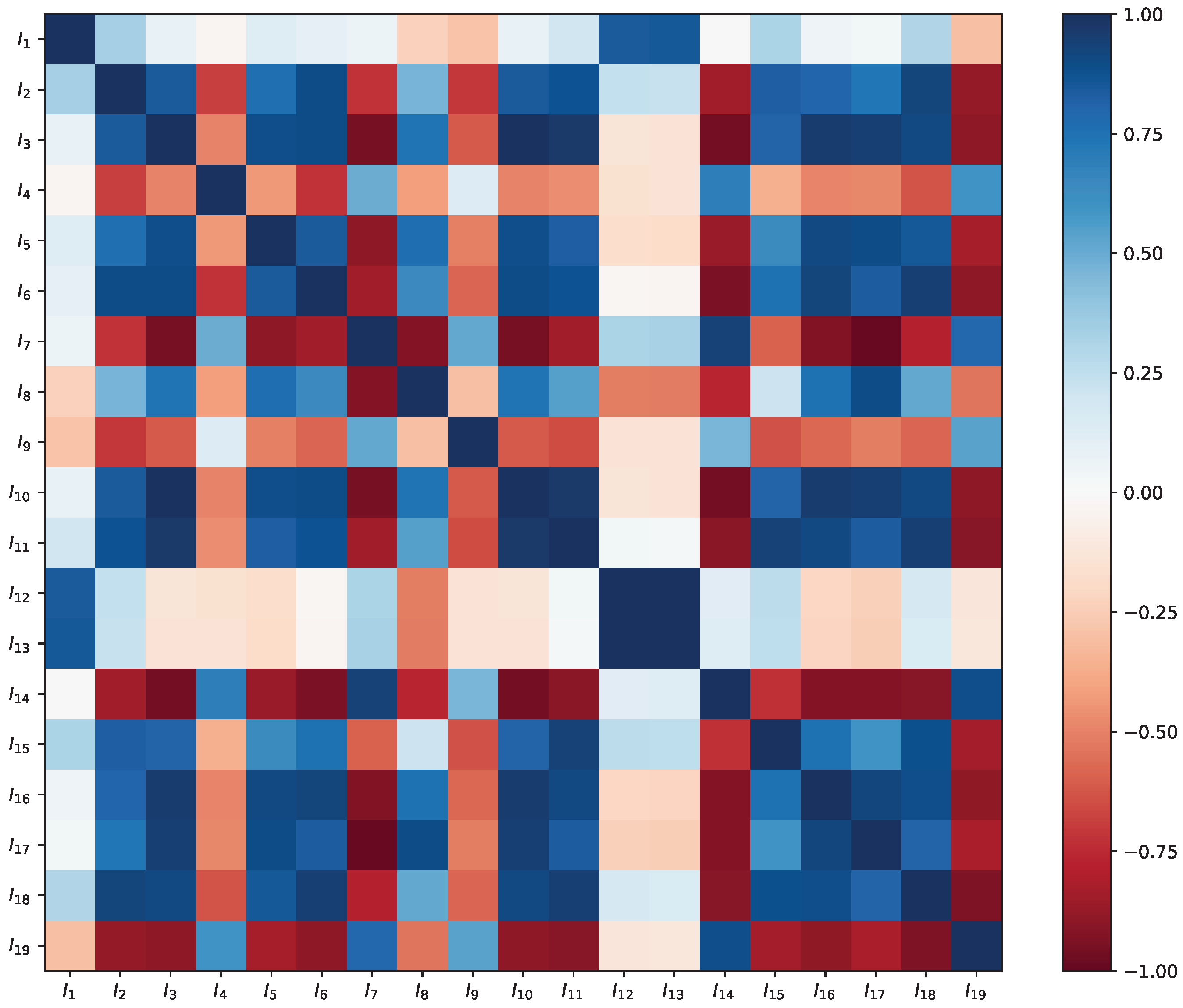
The analysis began with the examination of the standardized correlation matrix R, constructed from the selected environmental indicators. As illustrated in Figure 3, the matrix reveals significant off-diagonal structure, suggesting the presence of robust linear interdependencies among variables suitable for PCA.
The suitability of this matrix for factor analysis was formally confirmed. The KMO measure yielded a value of 0.6011, and Bartlett’s test of sphericity was statistically significant ( χ 2 ( 171 ) = 1430.58 ,   p < 0.0001 ). The assumption of linearity was also supported, with only 3 of the 171 indicator pairs showing potential non-linearity. While the Shapiro–Wilk test revealed some deviations from normality, this was not considered an impediment given the robustness of PCA to this assumption. Finally, a 5-fold cross-validation procedure confirmed the stability of the principal component, showing consistent explained variance (mean = 67.7 %, σ = 4.5 % ) and high similarity of the loading vectors (mean cosine similarity = 0.974).
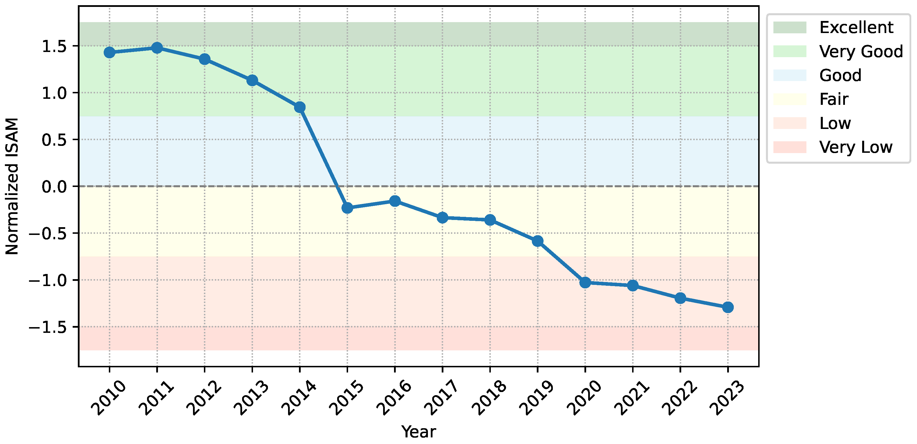
Having confirmed the data’s suitability and the component’s robustness, PCA was applied to calculate the RESI index. The first principal component alone explains a remarkable 66.85 % of the total variance across all 19 indicators, providing a solid foundation for the index as a synthesis of the system’s dominant dynamic. The evolution of this dynamic is presented in Figure 4, which shows the normalized scores for the period 2010–2023, classified into qualitative sustainability bands.

4.1. Construction of the Indicator Correlation Network

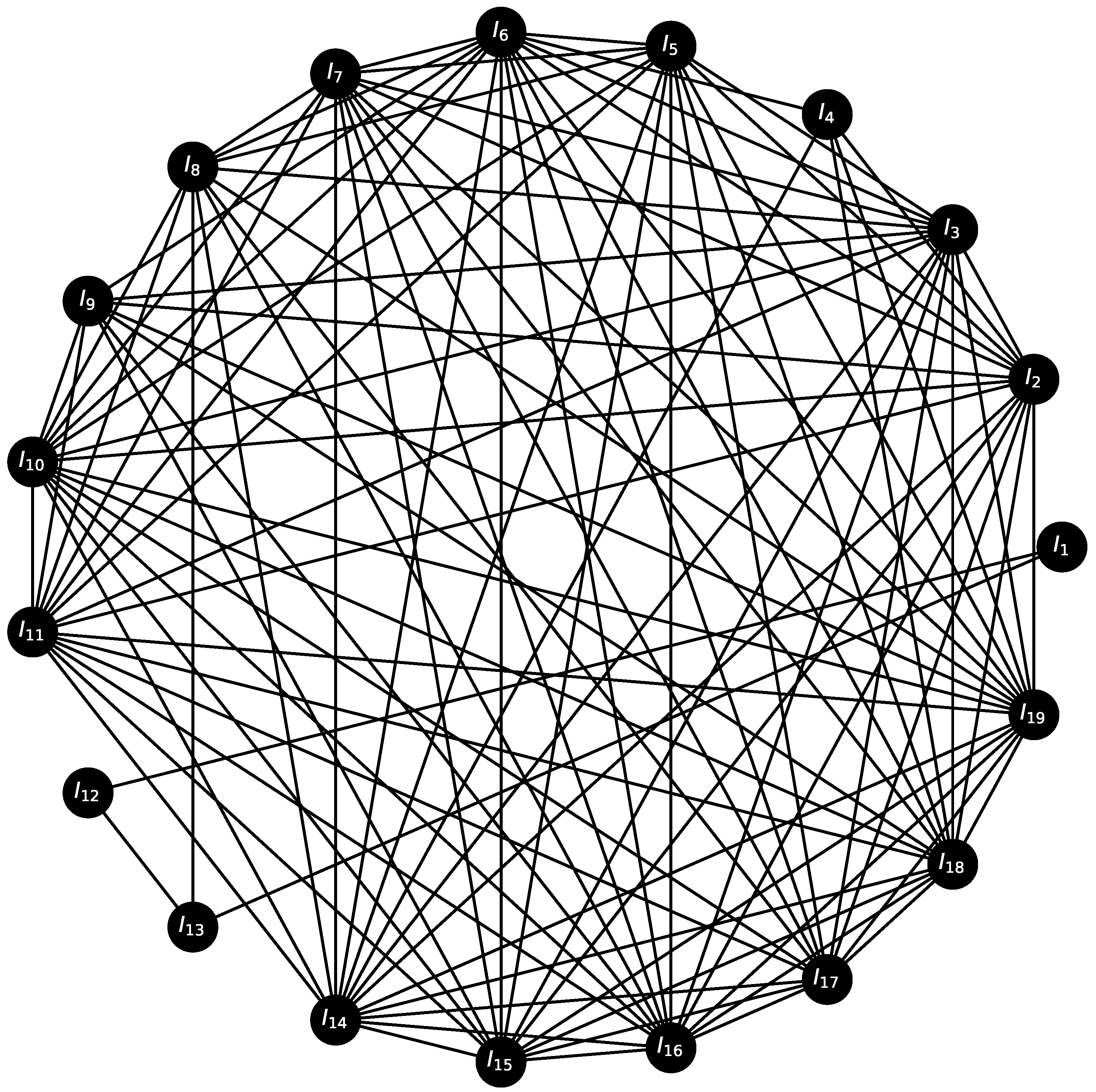
Applying the procedure described in the methodology, the correlation threshold required to maintain a fully connected network was determined to be τ = 0.5203 . This threshold filters for the most significant linear relationships among the indicators.
The resulting network, which captures these core patterns of co-variation, is visualized in Figure 5. In the figure, each node represents one of the 19 environmental indicators, and the links (edges) depict absolute correlations stronger than the calculated threshold.

4.2. Structural–Functional Cohesion Analysis

To assess the structural–functional cohesion of the indicator network, we computed the index M o ( G ) for the network constructed using a correlation threshold. The resulting network exhibits a density of d = 0.6199 , placing it near the upper–mid-range of the possible spectrum.
The node energy values, calculated via the spectral decomposition of the adjacency matrix, are reported in Table 3.
The corresponding shortest-path distance matrix among all node pairs is shown in Table 4.
Based on these inputs, the structural–functional cohesion index was computed as
M o ( G ) = 520.6804 .
Figure 6 illustrates the results of the sensitivity analysis. The plot confirms the robustness of the M o ( G ) index, which remains stable and exhibits no abrupt variations across the analyzed range of thresholds, τ [ 0.4703 ,   5203 ) , thereby validating the consistency of the structural diagnosis.

4.3. Global and Centrality Metrics

The indicator network’s global properties are summarized in Table 5. The analysis reveals a highly interconnected structure with 19 nodes and 106 links, resulting in a high link density ( d = 0.6199 ). The network is compact, evidenced by a small diameter (4) and a short average path length (1.64). A high global clustering coefficient ( C = 0.8880 ) indicates a strong tendency for indicators to form tightly connected groups. Community detection algorithms identified two distinct modules within the network.
Node-level analysis, detailed in Table 6, identifies the structural importance of individual indicators.

4.4. Comparative Analysis

To synthesize the findings from both the temporal and structural analyses, the contribution of each indicator to the respective indices was calculated. Table 7 presents the normalized importance scores for each indicator across three metrics: the first principal component ( Z 1 ) loading, the contribution to the M o ( G ) index, and degree centrality. Normalizing these values to a common [0, 1] scale allows for a direct comparison of an indicator’s importance in driving the temporal trend versus its role in maintaining the system’s structural cohesion.

4.5. Simulation Results

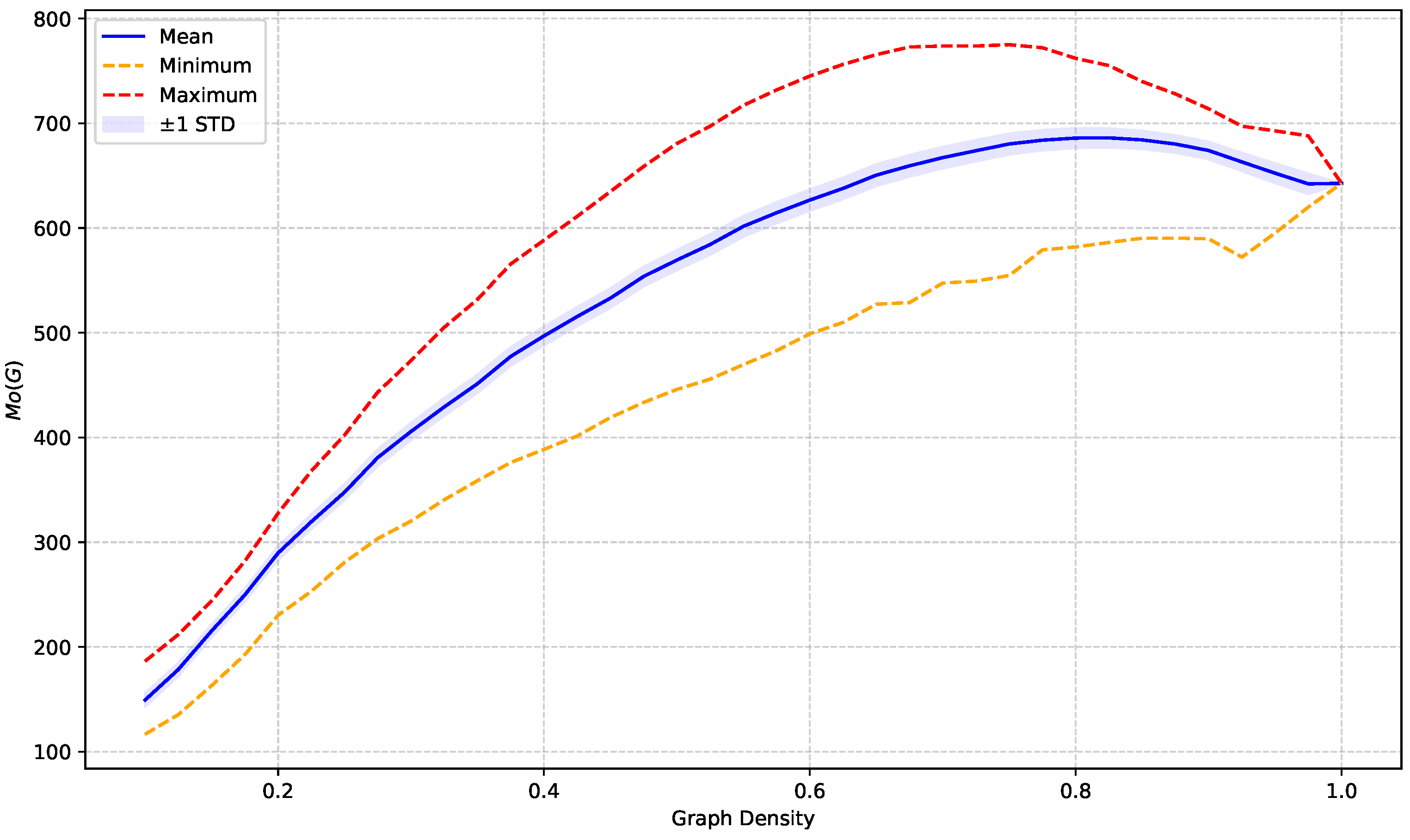
The behavior of the index M o ( G ) across all sampled network densities is summarized in Figure 7. The data exhibit a distinct nonlinear growth pattern, characterized by rapid initial increases followed by a gradual saturation and slight decline at higher densities. Starting from an average of approximately 149.39 at a density of 0.10, the index rises steadily, reflecting the progressive enrichment in structural connectivity as more links are added to the network. The mean value peaks at 685.93 near a density of 0.80, after which it slowly decreases, reaching 642.66 at a density of 1.00, the value associated with the complete network.
The standard deviation of M o ( G ) follows a similar trend, increasing with density up to a maximum of 10.24 at a density of 0.65, and subsequently declining as the network becomes more uniform. This behavior suggests that the index is particularly sensitive to the diversity of network configurations in the intermediate density range. At low densities, the variability is driven by the broad range of sparse but connected topologies. In contrast, as density approaches unity, the network structure becomes increasingly regular, leading to convergence in both shortest path lengths and node energies.
Across the full range of simulations, the minimum observed value of the index was 116.67, recorded at a density of 0.10, while the maximum value reached 775.10 at a density of 0.75. These extremes illustrate the capacity of the index to differentiate between poorly integrated and highly cohesive network structures. The wide spread of values in the intermediate densities reflects the combinatorial richness and structural variability of partially connected networks.
Notably, the region d [ 0.20 ,   0.75 ] marks a transitional phase where M o ( G ) grows rapidly and its variability remains high. This interval corresponds to the most pronounced structural transformations in the network, where the addition of links significantly enhances global cohesion. Beyond this range, further increases in density yield diminishing returns in terms of structural–functional integration, as reflected in the stabilization and eventual decline of the index.
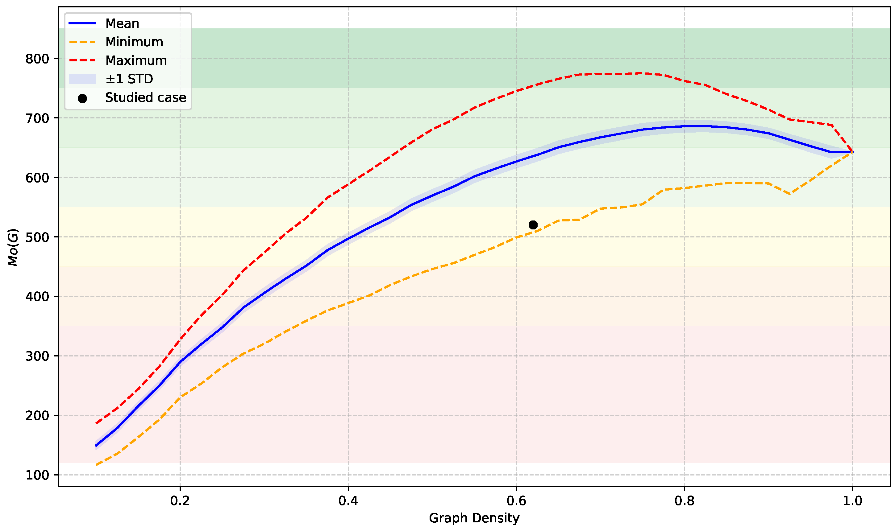
To support the interpretation of empirical values of M o ( G ) , we propose a qualitative classification that reflects the degree of structural integration within the network. This scheme is based on the empirical range of values obtained from simulations with n = 19 vertices and is consistent with the nonlinear growth and saturation behavior observed at higher densities. Table 8 summarizes this framework, in which different intervals of the index are associated with qualitative descriptors ranging from Very Poor to Excellent. These categories serve as a heuristic guide for evaluating the relative connectivity and organization of real-world systems in comparison with randomized connected networks of the same size.

5. Discussion

5.1. Interpretation of the RESI Trajectory

The 14-year trajectory of the RESI tells a clear story of progressive environmental decline, tracing the locality’s path from a period of relative stability to one of systemic crisis. This evolution reveals not a single event, but a series of interconnected pressures that gradually eroded the region’s socio-ecological resilience. The narrative can be understood in four distinct phases.
Between 2010 and 2012, the locality of Cruz Grande exhibited strong sustainability performance, with RESI values consistently falling within the Very Good range. This favorable condition reflected a confluence of efficient water governance, low per capita emissions, and high reforestation rates. These achievements were sustained by planned urban settlements, broad potable water coverage, and relatively stable ecological processes.
The decline began in 2013 and continued through 2015, during which the index dropped to the Fair range. This stage was marked by rapid urban expansion—often into aquifer recharge zones—an increase in untreated wastewater, and the weakening of environmental programs due to political transitions. Early droughts also contributed to yield reductions in irrigated agriculture, while fragmented planning led to increased pressure on natural systems.
From 2016 to 2018, the index continued its slow descent while remaining in the Fair range. During this period, systemic cohesion weakened, as evidenced by a sharp decline in the correlation between land-use and water indicators. Access to safe drinking water dropped significantly, leading to a rise in gastrointestinal illnesses, and deforestation rates increased while reforestation efforts became largely symbolic.
The years 2019 to 2023 saw a severe deterioration in performance, culminating in the lowest index value in 2023. This phase was shaped by overlapping crises: the COVID-19 pandemic caused infrastructural collapse, a spike in hazardous waste, and a slowdown in public environmental services. Simultaneously, prolonged droughts led to drastic reductions in crop productivity and a rise in poverty. The locality’s reliance on non-renewable energy deepened, while CO2 emissions per capita surged to critical levels.
The evolution of the index over this 14-year period reveals that temporary recoveries merely masked deeper vulnerabilities. The gradual disintegration of water–soil–energy linkages was a key driver of the systemic decline. Any sustainable recovery must focus on restoring these lost synergies and addressing the chronic governance and infrastructure gaps that allowed the sustainability profile to erode over time.

5.2. Interpretation of the M o ( G ) Value

This value falls squarely within the Fair category of structural integration, according to the classification proposed in Table 8 (see Figure 8). Notably, it lies close to the minimum observed value at its density level within the simulated benchmark ensemble ( min = 509.91 , mean = 637.88 at d = 0.625 ).
The relatively low structural–functional cohesion observed in the network, despite its moderate-to-high density, suggests a misalignment between local connectivity and global integrative capacity. That is, while the indicators are statistically interrelated (as evidenced by a large number of significant correlations), their structural arrangement does not favor an efficient distribution of influence across the system.
In spectral terms, this manifests as a dispersion of nodal energy values that is insufficiently channeled through short paths. Several nodes with high spectral prominence remain positioned at considerable topological distances from each other, diluting the aggregate pairwise energy-weighted closeness that defines M o ( G ) . Consequently, the system exhibits a form of latent fragmentation, where redundancies and peripheral links prevail over cohesive cores.
From a policy perspective, this result raises concerns. A territorial system with low structural–functional cohesion may suffer from limited resilience to systemic shocks, inefficient feedback among components, and a lack of synergies between key sustainability dimensions. In such contexts, decision-makers might consider re-evaluating indicator selection, improving data granularity, or exploring modular interventions aimed at enhancing integrative structure.
The comparison with the benchmark ensemble reinforces the singularity of this configuration. While most synthetic networks of comparable density achieve significantly higher values of M o ( G ) , the studied case emerges as an outlier. This indicates that its structural limitations are not a generic consequence of sparsity, but rather a reflection of the specific topology induced by the underlying indicator correlations.
These findings highlight the relevance of network-based diagnostics in sustainability analysis. Beyond the classical aggregation of indicator scores, the structural–functional cohesion index offers a complementary lens to detect inefficiencies in systemic structure that may hinder coherent territorial planning.

5.3. Integrated Analysis of the Network Structure

The analysis of the environmental indicator network provides a multidimensional perspective on systemic cohesion. A conventional structural analysis, relying on traditional metrics, would suggest the system is robust and well-integrated. For instance, the positive assortativity coefficient ( r = 0.3970 ) points to a resilient core of interconnected hubs, the extremely high global clustering coefficient ( C = 0.8880 ) indicates strong local cohesion, and the very low modularity ( Q = 0.0611 ) suggests the network resists fragmentation into separate communities. Taken together, these metrics portray a system with seemingly strong internal connectivity.
However, the structural–functional cohesion index M o ( G ) offers a starkly different and more nuanced diagnosis. Despite the indications of robustness from the metrics mentioned above, the index value of M o ( G ) = 520.68 places the network merely in the Fair category. This contrast highlights a key limitation of conventional metrics; while they effectively map patterns of connectivity, they may overlook deeper functional fragmentation. The M o ( G ) index, by weighting these connections by node energy and proximity, reveals that the network’s apparent structural cohesion does not translate into effective global integration.
Crucially, this more critical diagnosis provided by the M o ( G ) index is consistent with the region’s observed environmental performance. The RESI shows a marked decline from 2013 to 2023 (see Figure 4), reflecting a tangible weakening of systemic performance. This trend is corroborated by specific negative outcomes, such as decreased access to safe drinking water, accelerated forest cover loss, and rising per capita CO2 emissions. These dynamics validate the spectral analysis, confirming that the M o ( G ) index captures real-world vulnerabilities that the other metrics did not fully reveal.
The reason for this discrepancy lies in the distribution of influence within the network. High connectivity does not guarantee functional cohesion if the most influential nodes, as the node-level analysis reveals, are not positioned to act as effective integrators. Their impact can remain concentrated within local clusters, limiting their ability to foster global cohesion.
From a policy perspective, this insight is critical. Relying only on conventional metrics could lead to a false sense of security about the system’s resilience. Our findings demonstrate that effective governance requires moving beyond managing isolated indicators towards strategies that intentionally build functional bridges between different domains. This enhances the system’s overall structural–functional integration, a property captured by our index M o ( G ) .

5.4. Relative Importance of Indicators

The comparative analysis in the normalized Table 7 allows for a micro-level diagnosis of the system. It reveals the distinct roles played by each indicator in both the temporal decline and the structural (in)efficiency of the network.
A small set of indicators emerges as the true backbone of the system, scoring highly across all metrics. For example, I 3 (Access to water supply networks) and I 16 (Public water service wells) exhibit strong negative Z 1 loadings (−1.0000 and −0.9769, respectively), meaning their improvement is strongly associated with better sustainability outcomes. Crucially, they also have among the highest contributions to structural–functional cohesion (1.0000 and 0.9665, respectively) and are highly connected (a normalized degree centrality of 0.9232). These indicators are not just important in theory; they are central pillars that influence both the system’s performance and its structural integrity.
The analysis also identifies indicators that act as major hubs but whose influence on structural–functional cohesion is less than their connectivity suggests. I 6 (Water stress level) and I 19 (Forest and jungle coverage change) have the highest normalized degree centrality (1.0000), making them the most connected nodes. However, their contribution to the M o ( G ) index is more modest (0.7432 and 0.6826, respectively). This suggests they function as “local organizers” that connect many variables but are less critical for maintaining the efficient, global integration of the system compared to the true systemic backbone.
Perhaps the most critical finding is the identification of indicators that are actively driving the system’s negative performance. I 14 (Access to public transport), I 19 (Forest and jungle coverage change), and I 7 (Number of private wells) all have strong positive Z 1 loadings (0.9819, 0.9412, and 0.9431, respectively). This indicates that as these variables increased, the overall sustainability index declined. The network analysis reveals that these problem indicators are not isolated. In fact, they are highly connected within the system (with normalized degree centralities greater than 0.84). Their high connectivity provides a structural pathway for their negative influence to spread easily, making them essential targets for policy intervention.
Finally, the analysis confirms the existence of a functionally isolated periphery. Indicators I 1 (Environmental impact of agricultural activities) and I 12 (Land use efficiency) have negligible Z 1 loadings (normalized importance scores of −0.0884 and 0.0000, respectively) and the lowest contributions to both structural cohesion and connectivity (with all other normalized scores near 0.0000). They operate largely independently of the core dynamics governing the system’s decline, making them less relevant for understanding the primary feedback loops. This distinction, made possible by the hybrid analysis, allows for a more focused and strategic approach to managing the system.

6. Conclusions

This study reveals that the environmental sustainability of Cruz Grande, Guerrero, is in a critical situation. Its system of indicators, apparently well interconnected, suffers from profound structural and functional fragility. It is this weakness that has caused its sustained decline. By combining a temporal performance analysis with network theory, this research goes beyond traditional studies to uncover the hidden vulnerabilities that undermine the locality’s resilience.
There are two findings that support this conclusion. First, the RESI trajectory documents a clear and sustained deterioration in environmental performance observed between 2010 and 2023. This decline was characterized by the progressive erosion of vital synergies between water management, land use, and energy consumption, confirmed by data and field observations. Second, network analysis reveals the root cause of this fragility. Although the indicator network has a relatively high density ( d = 0.6199 ), our study, with a M o ( G ) value of 520.6804, places it in a merely Fair category, with significantly lower performance than networks of similar density. This disparity demonstrates that mere statistical connectivity does not guarantee structural–functional cohesion.
From a methodological point of view, this research presents a framework that matches the “what” of the decline (identified through PCA) with the “why” (explained through network analysis). The M o ( G ) index is presented as a measure of systemic structural–functional cohesion that complements and, in this case, explains the conclusions drawn from conventional metrics. The index proved to be mathematically robust, as its relationship with established indices in network theory was validated. Furthermore, computational simulations demonstrated its stable behavior across synthetic networks of varying densities, a process that enabled the development of the qualitative classification bands offered in this study as a practical tool for interpreting its results in other contexts.
From a public policy perspective, these findings call for a shift from sectoral solutions to integrated planning. The main challenge for Cruz Grande is not the lack of relationships between the indicators analyzed but their poor structural configuration. Our complementary analysis provides a nuanced roadmap for comprehensive intervention that goes beyond centrality to identify functions other than indicators. Effective governance must first focus on strengthening the backbone of the system, indicators such as I3 (Access to water supply networks) and I16 (Public water wells), which are essential in both time trend and structural–functional cohesion analyses. At the same time, policy must address the main factors of decline, such as I14 (Access to public transportation) and I7 (Number of private wells). Given their high connectivity, interventions to mitigate their negative impact would have positive ripple effects across the network. Finally, functionally isolated indicators, such as I1 (Impact of agricultural activities) and I12 (Land use efficiency), require a specific approach, perhaps managing them as a separate subsystem rather than forcing their integration into an already-inefficient system.
However, it is wise to recognize the limitations of the study associated with the data. Reliance on official data sources can present challenges in terms of accuracy and timeliness. To mitigate this limitation and ensure the contextual validity of the data, a rigorous three-level validation process was implemented to ensure the contextual validity of the indicators. Future work will focus on continuing to refine these metrics and applying this methodology to other regions of the state for comparative analysis.
Similarly, the implementation of these recommendations faces practical barriers. The use of Network Theory may hinder its adoption by decision-makers who are unfamiliar with this theory. To overcome this obstacle, it is necessary to develop intuitive tools and interpretive guides that translate the results into applicable diagnoses.
The transition to integrated planning also requires overcoming institutional barriers, such as administrative fragmentation, through participatory governance strategies. In this regard, the collaboration established with the local government of Cruz Grande is a key step. As a practical result of this partnership, a software tool will be delivered to the local administration. This tool is designed to enable policymakers to identify the most important indicators for the structural–functional cohesion of the system and determine which links should be strengthened or weakened to improve the overall structure of the network and thus promote the environmental sustainability of the region. The basic algorithms of this diagnostic tool are provided in pseudocode in Appendix C.

Author Contributions

Conceptualization, L.A.L., P.B., E.D.M., J.L.R.-A. and J.M.S.; methodology, L.A.L., P.B., E.D.M., J.L.R.-A. and J.M.S.; software, L.A.L., P.B., E.D.M., J.L.R.-A. and J.M.S.; validation, L.A.L., P.B., E.D.M., J.L.R.-A. and J.M.S.; formal analysis, L.A.L., P.B., E.D.M., J.L.R.-A. and J.M.S.; investigation, L.A.L., P.B., E.D.M., J.L.R.-A. and J.M.S.; writing—original draft preparation, L.A.L., P.B., E.D.M., J.L.R.-A. and J.M.S.; writing—review and editing, L.A.L., P.B., E.D.M., J.L.R.-A. and J.M.S.; visualization, L.A.L., P.B., E.D.M., J.L.R.-A. and J.M.S.; supervision, L.A.L., P.B., E.D.M., J.L.R.-A. and J.M.S.; project administration, L.A.L., P.B., E.D.M., J.L.R.-A. and J.M.S.; funding acquisition, L.A.L., P.B., E.D.M., J.L.R.-A. and J.M.S. All authors have read and agreed to the published version of the manuscript.

Funding

This research received no external funding.

Institutional Review Board Statement

Not applicable.

Informed Consent Statement

Not applicable.

Data Availability Statement

The raw data supporting the conclusions of this article will be made available by the authors on request.

Acknowledgments

We wish to express our sincere gratitude to the editors and the reviewers. Their rigorous review and insightful comments have greatly contributed to improving the clarity, structure, and robustness of this manuscript.

Conflicts of Interest

The authors declare no conflicts of interest.

Appendix A. Example

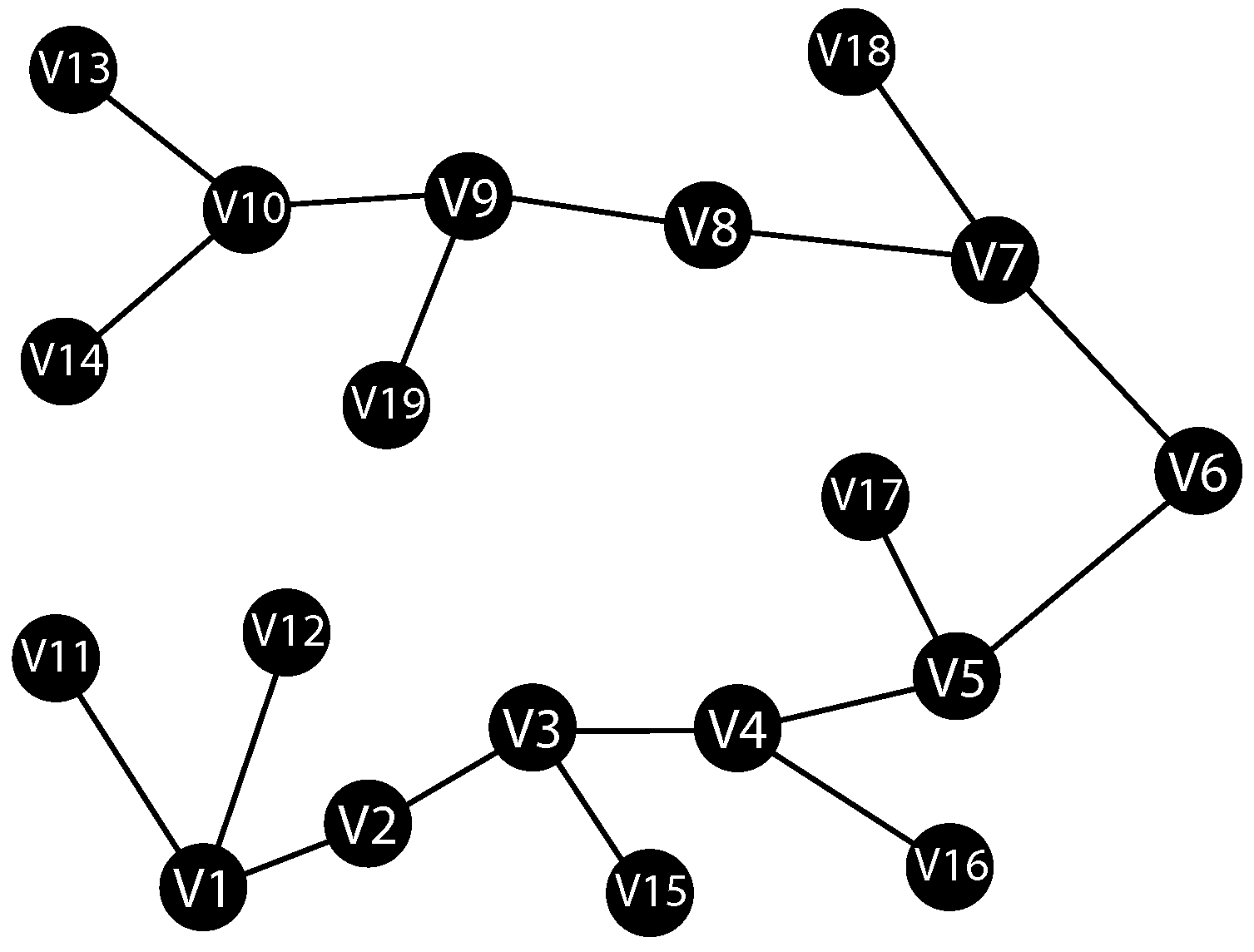
To illustrate the calculation of the M o ( G ) index, we construct a connected network consisting of n = 19 nodes and m = 18 links. This example allows for an explicit examination of the spectral and topological components that define the index.
Figure A1 shows the structure of the example network. Each node is labeled v i for i = 1 ,   ,   19 .
Figure A1. Example network used to compute the index M o ( G ) .
Sustainability 17 09731 g0a1
Based on this configuration, we computed the adjacency matrix and the eigenvalues and eigenvectors to obtain the node energies according to Equation (10). The resulting values, are presented in Table A1. These energies reflect the contribution of each node to the global spectral profile of the network, with higher values indicating nodes that are more structurally embedded or influential.
Table A1. Node energy values ε u for each node in the example network.
Node v i Energy ε v i
v 1 1.704420
v 2 1.051103
v 3 1.643572
v 4 1.585851
v 5 1.641706
v 6 1.068823
v 7 1.673259
v 8 1.073220
v 9 1.633139
v 10 1.669713
v 11 0.612690
v 12 0.612690
v 13 0.664017
v 14 0.664017
v 15 0.705714
v 16 0.853167
v 17 0.713735
v 18 0.660393
v 19 0.723364
Intuitively, a node’s energy measures its “importance” within the network’s structure. A node with high energy, such as v 1 (1.705) and v 7 (1.673), is not only well-connected but is positioned in a way that significantly influences the global properties and stability of the entire network. Conversely, a node with low energy like v 1 1 and v 1 2 (0.613) is structurally peripheral.
Simultaneously, we computed the shortest-path distance between all pairs of nodes using standard network traversal algorithms. The corresponding distance matrix is shown in Table A2. These distances serve to weight the energy contributions in the definition of M o ( G ) .
Table A2. Shortest-path distance matrix d ( u , v ) among all node pairs in the example network.
v 1 v 2 v 3 v 4 v 5 v 6 v 7 v 8 v 9 v 10 v 11 v 12 v 13 v 14 v 15 v 16 v 17 v 18 v 19
v 1 012345678911101034569
v 2 1012345678229923458
v 3 2101234567338812347
v 4 3210123456447721236
v 5 4321012345556632125
v 6 5432101234665543214
v 7 6543210123774454323
v 8 7654321012883365432
v 9 8765432101992276541
v 10 987654321010101187652
v 11 12345678910021111456710
v 12 12345678910201111456710
v 13 1098765432111110298763
v 14 1098765432111112098763
v 15 3212345678449903458
v 16 4321234567558830347
v 17 5432123456667743036
v 18 6543212345776654305
v 19 987654321210103387650
The diagonal of the distance matrix (from v 1 to v 1 , etc.) contains zeros because the distance from a node to itself is, by definition, zero. No steps are required to travel from a node to itself.
Combining the information from both Table A1 and Table A2; and following Equation (11), we compute the contribution of each unordered pair of nodes to the index M o ( G ) . These pairwise terms are shown in Table A3, where each entry represents the value ( ε u + ε v ) / d ( u , v ) for the corresponding node pair.
Table A3. Pairwise contributions ( ε u + ε v ) / d ( u , v ) to the index M o ( G ) in the example network.
v 1 v 2 v 3 v 4 v 5 v 6 v 7 v 8 v 9 v 10 v 11 v 12 v 13 v 14 v 15 v 16 v 17 v 18 v 19
v 1 2.761.671.100.840.550.560.400.420.372.322.320.240.240.800.640.480.340.27
v 2 2.691.320.900.530.540.350.370.310.830.830.190.190.880.630.440.290.22
v 3 3.231.640.900.830.540.550.471.081.080.290.292.351.250.790.460.34
v 4 3.231.331.090.660.640.531.051.050.320.321.152.441.150.560.38
v 5 2.711.660.900.820.660.450.450.380.380.781.252.360.770.47
v 6 2.741.070.900.680.280.280.350.350.440.640.890.860.45
v 7 2.751.651.110.330.330.580.580.480.630.802.330.80
v 8 2.711.370.210.210.580.580.300.390.450.870.90
v 9 3.300.250.251.151.150.330.410.470.762.36
v 10 0.230.232.332.330.300.360.400.581.20
v 11 0.610.120.120.330.290.220.160.13
v 12 0.120.120.330.290.220.160.13
v 13 0.660.150.190.200.260.46
v 14 0.150.190.200.260.46
v 15 0.520.350.230.18
v 16 0.520.300.23
v 17 0.340.24
v 18 0.35
v 19
The table of contributions is presented as an upper triangular matrix because the calculation is symmetrical. The contribution of the pair ( v 1 , v 2 ) is identical to that of the pair ( v 2 , v 1 ) . To avoid redundancy in the display and double-counting during summation, only the contributions for unordered pairs { u , v } are calculated and shown.
The values presented in Table A3 reveal a clear differentiation in the magnitude of contributions among node pairs. Notably, the largest terms correspond to nodes that are both energetically significant and topologically close. For example, the pair ( v 3 , v 4 ) yields the highest contribution ( 3.23 ), driven by the combination of strong node energies ( ε v 3 = 1.644 , ε v 4 = 1.586 ) and a minimal path length of 1. Similarly, pairs such as ( v 4 , v 5 ) and ( v 9 , v 10 ) also exhibit high contributions due to their favorable spectral and spatial properties. In contrast, distant and weakly energetic nodes, such as ( v 1 , v 19 ) or ( v 11 , v 14 ) , contribute far less to the total index.
Summing all unique pairwise terms yields the final value of the index for this illustrative example,
M o ( G ) = 131.3424 .
The final value, M o ( G ) = 131.3424 , represents the total structural–functional cohesion of the network. A higher value would indicate a more “efficient” network, where important nodes (those with high energy) are very close to one another. A lower value would suggest a more fragmented structure, where important nodes are topologically distant. This value by itself is useful for comparing different networks; for a qualitative interpretation, it must be compared against the benchmark values obtained from a computational study or empirical results. For this sample network, the M o ( G ) value falls into the “Very Poor” category, near the minimum observed value in Section 4.5. This indicates that the network is highly fragile and suboptimally structured.

Appendix B. Proofs of Theoretical Results

Proof of Proposition 1.
We begin with the definition of the M o ( G ) index, which is a sum over all unordered pairs of distinct nodes { u , v } V ( G ) . We can rewrite this sum and regroup the terms by each node. Let V ( G ) = { v 1 , , v n } , then
M o ( G ) = u v ε u + ε v d ( u , v ) = 1 i < j n ε v i + ε v j d ( v i , v j ) = 1 i < j n ε v i d ( v i , v j ) + 1 i < j n ε v j d ( v i , v j ) .
In this form, the expression consists of two symmetric sums. We can combine them by regrouping the terms for each mode v k , where k ranges from 1 to n. For a given node v k , its energy ε v k appears in the sum whenever it is paired with any other node v i (where i k ).
M o ( G ) = k = 1 n i = 1 , i k n ε v k d ( v k , v i ) = k = 1 n ε v k i = 1 , i k n 1 d ( v k , v i ) .
This final expression is a sum over the nodes of the graph. Removing the explicit numbering, we can write the result for any node v V ( G )
M o ( G ) = v V ( G ) ε v u v 1 d ( u , v ) .
which completes the proof.    □
Proof of Proposition 2.
Let V ( G ) = { v 1 , , v n } . By definition of the index,
M o ( G ) = 1 i < j n ε v i + ε v j d ( v i , v j ) .
Since the network is connected, we have 1 d ( v i , v j ) diam ( G ) for all i j . It follows that
ε v i + ε v j diam ( G ) ε v i + ε v j d ( v i , v j ) ε v i + ε v j .
Hence,
1 diam ( G ) 1 i < j n ε v i + ε v j M o ( G ) 1 i < j n ε v i + ε v j .
We now evaluate the sum 1 i < j n ε v i + ε v j . This expression can be split as
1 i < j n ε v i + ε v j = 1 i < j n ε v i + 1 i < j n ε v j .
In the first sum, each ε v i appears exactly n i times (once for each j > i ), and in the second sum, each ε v j appears j 1 times (once for each i < j ). Therefore,
1 i < j n ε v i + ε v j = i = 1 n ε v i ( n i ) + j = 1 n ε v j ( j 1 ) .
Combining both terms, we obtain,
1 i < j n ε v i + ε v j = k = 1 n ε v k ( n k ) + ( k 1 ) = k = 1 n ε v k ( n 1 ) .
Thus, the index satisfies,
( n 1 ) diam ( G ) k = 1 n ε v k M o ( G ) ( n 1 ) k = 1 n ε v k .
   □
Proof of Proposition 3.
By Equation (15), for any node pair u v ,
1 Δ ( d u + d v ) ε u + ε v d u + d v .
Dividing by d ( u , v ) , we obtain
1 Δ · d u + d v d ( u , v ) ε u + ε v d ( u , v ) d u + d v d ( u , v ) .
Summing over all unordered pairs of distinct nodes { u , v } , yields the desired bounds.    □
Proof of Proposition 4.
From Proposition 3 we know that
1 Δ u v d u + d v d ( u , v ) M o ( G ) u v d u + d v d ( u , v ) .
We now split the sum over all unordered pairs of distinct nodes into two parts, those that form edges and those that do not.
u v d u + d v d ( u , v ) = u v E ( G ) d u + d v d ( u , v ) + u v E ( G ) d u + d v d ( u , v ) .
If u v E ( G ) then d ( u , v ) = 1 , and the first sum becomes
u v E ( G ) ( d u + d v ) = M 1 3 / 2 ( G ) .
On the other hand, for u v E ( G ) we have 2 d ( u , v ) diam ( G ) . Also, since δ d u , d v Δ , it follows that
2 δ d u + d v 2 Δ .
We now estimate the second sum. For the upper bound,
u v E ( G ) d u + d v d ( u , v ) Δ u v E ( G ) 1 = Δ n 2 m .
For the lower bound,
u v E ( G ) d u + d v d ( u , v ) 2 δ diam ( G ) n 2 m .
Combining these estimates, we obtain the desired inequalities.    □
Proof of Proposition 5.
Note that for all node pair u v ,
2 δ d u + d v 2 Δ .
So, dividing by d ( u , v ) , we get
2 δ · 1 d ( u , v ) d u + d v d ( u , v ) 2 Δ · 1 d ( u , v ) .
Summing over all unordered pairs of distinct nodes { u , v } , we obtain
2 δ u v 1 d ( u , v ) u v d u + d v d ( u , v ) 2 Δ u v 1 d ( u , v )
The result follows from Proposition 3.    □
Proof of Proposition 6.
For the lower bound, we first apply the Cauchy–Schwarz inequality to the sequences a i = d ( u , v ) and b i = 1 / d ( u , v ) , where the index i runs over all unordered node pairs { u , v } V ( G ) . The inequality states that
i = 1 k a i b i 2 i = 1 k a i 2 i = 1 k b i 2 ,
Applying this inequality, we obtain
W ( G ) H ( G ) = u v d ( u , v ) u v 1 d ( u , v ) u v d ( u , v ) · 1 d ( u , v ) 2 = n 2 2 .
This yields the bound
H ( G ) n 2 ( n 1 ) 2 4 W ( G ) .
Combining this result with the lower bound for M o ( G ) given in Equation (20), we conclude that
M o ( G ) 2 δ Δ H ( G ) δ n 2 ( n 1 ) 2 2 Δ W ( G ) .
For the upper bound, we use the Kantorovich inequality, which states that if a 1 , , a k are positive real numbers such that r a i R for all i, then
i = 1 k a i i = 1 k 1 a i ( R + r ) 2 k 2 4 r R ,
with equality if and only if r = R . In our setting, we apply this to the values a i = d ( u , v ) , with r = 1 , R = D , and k = n 2 , obtaining
W ( G ) H ( G ) = u v d ( u , v ) u v 1 d ( u , v ) n 2 ( n 1 ) 2 ( D + 1 ) 2 16 D .
Therefore,
H ( G ) n 2 ( n 1 ) 2 ( D + 1 ) 2 16 D W ( G ) .
Substituting this into the upper bound from Equation (20), we arrive at
M o ( G ) 2 Δ H ( G ) Δ n 2 ( n 1 ) 2 ( D + 1 ) 2 8 D W ( G ) .
   □

Appendix C. Algorithms

Algorithm A1 Ranking Nodes by Contribution to Systemic Cohesion ( M o ( G ) )
Require: 
A connected graph G = ( V , E ) .
Ensure: 
A list of nodes L ranked , sorted in descending order by their contribution to M o ( G ) .
 1:
procedure RankByMoContribution(G)
 2:
                              ▹ 1. Compute base metrics
 3:
     ϵ VertexEnergies ( G ) .
 4:
     D DistanceMatrix ( G ) .
 5:
                           ▹ 2. Calculate Mo(G) contributions
 6:
    Initialize an empty map C Mo to store contributions.
 7:
    for each node v V  do
 8:
         S v u V , u v 1 D v u                     ▹ Sum of inverse distances
 9:
         C Mo ( v ) ϵ v × S v                       ▹ Contribution of node v
10:
    end for
11:
                     ▹ 3. Sort nodes by their calculated contribution
12:
     L ranked SortDescending ( V , by   C Mo )
13:
    return  L ranked
14:
end procedure
Algorithm A2 Structural Optimization for Cohesion ( M o ( G ) )
Require: 
A connected graph G = ( V , E ) .
Ensure: 
Two sorted lists: L additions and L removals .
 1:
procedure OptimizeCohesionMoG(G)
 2:
     M o initial M o ( G )
 3:
     L additions
 4:
     L removals
 5:
                              ▹ 1. Evaluate edge additions
 6:
     E potential { ( u , v ) u , v V , u v , ( u , v ) E }
 7:
    for  a E potential  do
 8:
         G ( V , E { a } )
 9:
         Δ M o M o ( G ) M o initial
10:
        if  Δ M o > 0  then
11:
           Append ( a , Δ M o ) to L additions
12:
        end if
13:
    end for
14:
                              ▹ 2. Evaluate edge removals
15:
    for  s E  do
16:
         G ( V , E { s } )
17:
        if IsConnected ( G )  then
18:
            Δ M o M o ( G ) M o initial
19:
           if  Δ M o > 0  then
20:
               Append ( s , Δ M o ) to L removals
21:
           end if
22:
        end if
23:
    end for
24:
                                    ▹ 3. Sort results
25:
     L additions SortDescending ( L additions , by   Δ M o )
26:
     L removals SortDescending ( L removals , by   Δ M o )
27:
    return  { L additions , L removals }
28:
end procedure

References

  1. World Commission on Environment and Development (WCED). Our Common Future; Oxford University Press: Oxford, UK, 1987. [Google Scholar]
  2. Kates, R.W.; Parris, T.M.; Leiserowitz, A.A. What is Sustainable Development? Goals, Indicators, Values, and Practice. Environ. Sci. Policy Sustain. Dev. 2005, 47, 8–21. [Google Scholar] [CrossRef]
  3. Brito, R.M.; Rodriguez, C.; Sampedro, M.; Aparicio, J. Indicadores de sustentabilidad en las funciones sustantivas de la UAGro. Rev. Iberoam. Investig. Desarro. Educ. 2018, 8, 34–38. [Google Scholar]
  4. Singh, R.K.; Murty, H.; Gupta, S.; Dikshit, A. An overview of sustainability assessment methodologies. Ecol. Indic. 2009, 9, 189–212. [Google Scholar] [CrossRef]
  5. Greco, S.; Ishizaka, A.; Tasiou, M.; Torrisi, G. On the methodological framework of composite indices: A review of the issues of weighting, aggregation, and robustness. Soc. Indic. Res. 2019, 141, 61–94. [Google Scholar] [CrossRef]
  6. United Nations Development Programme. Human Development Report 1990: Concept and Measurement of Human Development; Oxford University Press: New York, NY, USA, 1990. [Google Scholar]
  7. World Economic Forum; Yale Center for Environmental Law and Policy; Center for International Earth Science Information Network (CIESIN), Columbia University. 2002 Environmental Sustainability Index; Yale University: New Haven, CT, USA, 2002. [Google Scholar]
  8. Esty, D.C.; Levy, M.A.; Srebotnjak, T.; de Sherbinin, A.; Kim, C.H.; Anderson, B. 2006 Environmental Performance Index; Yale Center for Environmental Law and Policy: New Haven, CT, USA, 2006. [Google Scholar]
  9. Schlör, H.; Fischer, W.; Hake, J.F. ISD: A New Methodological Approach for Measuring the Sustainability of the German Energy System. Ecol. Res. Int. 2011, 2011, 872048. [Google Scholar] [CrossRef]
  10. Biggeri, M.; Mauro, V. Towards a more ’Sustainable’ Human Development Index: Integrating the environment and freedom. Ecol. Indic. 2018, 91, 220–231. [Google Scholar] [CrossRef]
  11. Garibaldi Trejo, L.A.; Espinosa, J.; Ríos, A.; López, M. Coproducción de conocimiento socioambiental en la subcuenca Río La Sabana–Laguna de Tres Palos. Acta Univ. 2024, 34, e4083. [Google Scholar]
  12. Sánchez-Duarte, N.E.; Bracamontes-Nevárez, J.; Álvarez-Chávez, C.R. Socio-economic development and environmental sustainability in urban municipalities of the Northwestern Region of Mexico. Estud. Soc. Rev. Aliment. Contemp. Desarro. Reg. 2020, 30, e20868. [Google Scholar]
  13. West, S.; Haider, L.J.; Stålhammar, S.; Woroniecki, S. A relational turn for sustainability science? Relational thinking, leverage points and transformations. Ecosyst. People 2020, 161, 304–325. [Google Scholar] [CrossRef]
  14. Bodin, Ö.; Alexander, S.M.; Baggio, J.; Barnes, M.L.; Berardo, R.; Cumming, G.S.; Dee, L.E.; Fischer, A.P.; Fischer, M.; Garcia, M.M.; et al. Improving network approaches to the study of complex social-ecological interdependencies. Nat. Sustain. 2019, 2, 551–559. [Google Scholar] [CrossRef]
  15. Folke, C.; Jansson, A.; Rockström, J.; Olsson, P.; Carpenter, S.R.; Chapin, F.S., 3rd; Crépin, A.-S.; Daily, G.; Danell, K.; Ebbesson, J.; et al. Reconnecting to the biosphere. AMBIO 2011, 40, 719–738. [Google Scholar] [CrossRef] [PubMed]
  16. Bascompte, J.; Jordano, P.; Melián, C.J.; Olesen, J.M. The nested assembly of plant–animal mutualistic networks. Proc. Natl. Acad. Sci. USA 2003, 100, 9383–9387. [Google Scholar] [CrossRef]
  17. Jordano, P.; Bascompte, J.; Olesen, J.M. Invariant properties in coevolutionary networks of plant–animal links. Ecol. Lett. 2003, 6, 69–81. [Google Scholar] [CrossRef]
  18. Dale, M.R.T. Applying Graph Theory in Ecological Research; Cambridge University Press: Cambridge, UK, 2017. [Google Scholar]
  19. Aquilué, N.; Filotas, É.; Craven, D.; Fortin, M.J.; Brotons, L.; Messier, C. Evaluating forest resilience to global threats using functional response traits and network properties. Ecol. Appl. 2020, 30, e02095. [Google Scholar] [CrossRef]
  20. Levin, S.A. Ecosystems and the biosphere as complex adaptive systems. Ecosystems 1998, 1, 431–436. [Google Scholar] [CrossRef]
  21. Ostrom, E. A general framework for analyzing sustainability of social-ecological systems. Science 2009, 325, 419–422. [Google Scholar] [CrossRef]
  22. Gonzalès, R.; Parrott, L. Network theory in the assessment of the sustainability of social–ecological systems. Geogr. Compass 2012, 6, 76–88. [Google Scholar] [CrossRef]
  23. Sayles, J.S.; Mancilla Garcia, M.; Hamilton, M.; Alexander, S.M.; Baggio, J.A.; Fischer, A.P.; Ingold, K.; Meredith, G.R.; Pittman, J. Social-ecological network analysis for sustainability sciences: A systematic review and innovative research agenda for the future. Environ. Res. Lett. 2019, 14, 093003. [Google Scholar] [CrossRef]
  24. Janssen, M.A.; Bodin, Ö.; Anderies, J.M.; Elmqvist, T.; Ernstson, H.; McAllister, R.R.; Olsson, P.; Ryan, P. Toward a network perspective of the study of resilience in social-ecological systems. Ecol. Soc. 2006, 11, 15. [Google Scholar] [CrossRef]
  25. Norberg, J.; Cumming, G. Complexity Theory for a Sustainable Future; Columbia University Press: New York, NY, USA, 2008. [Google Scholar]
  26. Barnes, M.L.; Bodin, Ö.; Guerrero, A.M.; McAllister, R.R.; Alexander, S.M.; Robins, G. The social structural foundations of adaptation and transformation in social–ecological systems. Ecol. Soc. 2017, 22, 16. [Google Scholar] [CrossRef]
  27. Bodin, Ö.; Tengö, M. Disentangling intangible social–ecological systems. Glob. Environ. Change 2012, 22, 430–439. [Google Scholar] [CrossRef]
  28. Hamilton, M.; Fischer, A.P.; Ager, A. A social-ecological network approach for understanding wildfire risk governance. Glob. Environ. Change 2019, 54, 113–123. [Google Scholar] [CrossRef]
  29. Raj, U.; Banerjee, A.; Ray, S.; Bhattacharya, S. Structure of higher-order interactions in social-ecological networks through Q-analysis of their neighbourhood and clique complex. PLoS ONE 2024, 19, e0306409. [Google Scholar] [CrossRef] [PubMed]
  30. Bodin, Ö.; Crona, B.I. The role of social networks in natural resource governance: What relational patterns make a difference? Glob. Environ. Change 2009, 19, 366–374. [Google Scholar] [CrossRef]
  31. Franco-Gaviria, F.; Amador-Jiménez, M.; Millner, N.; Durden, C.; Urrego, D.H. Quantifying resilience of socio-ecological systems through dynamic Bayesian networks. Front. For. Glob. Change 2022, 5, 889274. [Google Scholar] [CrossRef]
  32. Aguilar-Becerra, C.D.; Frausto-Martínez, O.; Avilés-Pineda, H.; Pineda-Pineda, J.J.; Soares, J.C.; Reyes-Umaña, M. Path dependence and social network analysis on evolutionary dynamics of tourism in coastal rural communities. Sustainability 2019, 11, 4854. [Google Scholar] [CrossRef]
  33. Pineda-Pineda, J.J.; Martínez-Martínez, C.T.; Méndez-Bermúdez, J.A.; Muñoz-Rojas, J.; Sigarreta, J.M. Application of bipartite networks to the study of water quality. Sustainability 2020, 12, 5143. [Google Scholar] [CrossRef]
  34. Larrea-Gallegos, G.; Benetto, E.; Marvuglia, A.; Navarrete Gutiérrez, T. Sustainability, resilience and complexity in supply networks: A literature review and a proposal for an integrated agent-based approach. Sustain. Prod. Consum. 2022, 30, 946–961. [Google Scholar] [CrossRef]
  35. Kim, J.; Allenby, B. Development of sustainability network theory (SNT) and model for managing electronics industrial system. IEEE Int. Symp. Electron. Environ. 2007, 170–173. [Google Scholar] [CrossRef]
  36. Nilsson, M.; Griggs, D.; Visbeck, M. Policy: Map the interactions between Sustainable Development Goals. Nature 2016, 534, 320–322. [Google Scholar] [CrossRef]
  37. Benhar, O.; Fantoni, S.; Lovato, A. Complex network theory applied to sustainability. In Complex Systems with Artificial Intelligence–Sustainability and Self-Constitution; IntechOpen: London, UK, 2024. [Google Scholar]
  38. Dragicevic, A.Z. Concentric framework for sustainability assessment. J. Clean. Prod. 2020, 248, 119268. [Google Scholar] [CrossRef]
  39. Aka, K.G. Actor-network theory-based applications in sustainability: A systematic literature review. Clean. Prod. Lett. 2025, 8, 100084. [Google Scholar] [CrossRef]
  40. Liu, J.; Hull, V.; Batistella, M.; DeFries, R.; Dietz, T.; Fu, F.; Hertel, T.W.; Izaurralde, R.C.; Lambin, E.F.; Li, S.; et al. Framing sustainability in a telecoupled world. Ecol. Soc. 2013, 18, 26. [Google Scholar] [CrossRef]
  41. Barabási, A.L. Linked: The New Science of Networks; Perseus Publishing: Cambridge, MA, USA, 2003. [Google Scholar]
  42. Jolliffe, I.T. Principal Component Analysis; Springer Series in Statistics; Springer: New York, NY, USA, 2002. [Google Scholar]
  43. Abdi, H.; Williams, L.J. Principal component analysis. WIREs Comput. Stat. 2010, 2, 433–459. [Google Scholar] [CrossRef]
  44. Dunteman, G.H. Principal Components Analysis; Quantitative Applications in the Social Sciences; SAGE Publications, Inc.: Sussex, CA, USA, 1989. [Google Scholar]
  45. Jiang, Q.; Liu, Z.; Liu, W.; Li, T.; Cong, W.; Zhang, H.; Shi, J. A principal component analysis based three-dimensional sustainability assessment model to evaluate corporate sustainable performance. J. Clean. Prod. 2018, 187, 625–637. [Google Scholar] [CrossRef]
  46. Malah, A.; Bahi, H. Integrated multivariate data analysis for Urban Sustainability Assessment, a case study of Casablanca city. Sustain. Cities Soc. 2022, 86, 104100. [Google Scholar] [CrossRef]
  47. Kaiser, H.F. An index of factorial simplicity. Psychometrika 1974, 39, 31–36. [Google Scholar] [CrossRef]
  48. Horn, J.L. A rationale and test for the number of factors in factor analysis. Psychometrika 1965, 30, 179–185. [Google Scholar] [CrossRef]
  49. Velicer, W.F. Determining the number of components from the matrix of partial correlations. Psychometrika 1976, 41, 321–327. [Google Scholar] [CrossRef]
  50. Jackson, D.A. Stopping rules in principal components analysis: A comparison of heuristics and criteria. Ecology 1993, 74, 2204–2214. [Google Scholar] [CrossRef]
  51. Nardo, M.; Saisana, M.; Saltelli, A.; Tarantola, S.; Hoffman, A.; Giovannini, E. Handbook on Constructing Composite Indicators: Methodology and User Guide; OECD Publishing: Paris, France; European Commission Joint Research Centre: Ispra, Italy, 2005. [Google Scholar]
  52. Filmer, D.; Pritchett, L.H. Estimating wealth effects without expenditure data—Or tears: An application to educational enrollments in states of India. Demography 2001, 38, 115–132. [Google Scholar] [CrossRef] [PubMed]
  53. Vyas, S.; Kumaranayake, L. Constructing socio-economic status indices: How to use principal components analysis. Health Policy Plan. 2006, 21, 459–468. [Google Scholar] [CrossRef]
  54. Mazziotta, M.; Pareto, A. Principal component analysis for constructing socio-economic composite indicators: Theoretical and empirical considerations. SN Soc. Sci. 2024, 4, 114. [Google Scholar] [CrossRef]
  55. Newman, M.E.J. Networks: An Introduction, 2nd ed.; Oxford University Press: Oxford, UK, 2010. [Google Scholar]
  56. Arizmendi, O.; Hidalgo, J.F.; Juarez–Romero, O. Energy of a node. Linear Algebra Appl. 2018, 557, 449–455. [Google Scholar] [CrossRef]
  57. Gutman, I. The energy of a graph. Ber. Math.-Statist. Sekt. Forschungsz. Graz 1978, 103, 1–22. [Google Scholar]
  58. Li, X.; Zheng, J. A Unified Approach to the Extremal Trees for Different Indices. MATCH Commun. Math. Comput. Chem. 2005, 54, 195–208. [Google Scholar]
  59. Plavšić, D.; Nikolić, S.; Trinajstić, N.; Mihalić, Z. On the Harary index for the characterization of chemical graphs. J. Math. Chem. 1993, 12, 235–250. [Google Scholar] [CrossRef]
  60. Wiener, H. Structural determination of paraffin boiling points. J. Am. Chem. Soc. 1947, 69, 17–20. [Google Scholar] [CrossRef]
  61. H. Ayuntamiento Municipal Constitucional de Florencio Villarreal. Plan Municipal de Desarrollo 2021–2024; H. Ayuntamiento Municipal Constitucional de Florencio Villarreal: Cruz Grande, Guerrero, Mexico, 2021. [Google Scholar]
  62. Instituto Nacional de Estadística y Geografía (INEGI). Marco Geoestadístico Municipal 2010, version 4.3; INEGI: Aguascalientes, Mexico, 2010.
  63. Servicio de Información Agroalimentaria y Pesquera (SIAP). Sistema de Información Agroalimentaria de Consulta (SIACON). Available online: https://www.gob.mx/siap/acciones-y-programas/siacon-ng (accessed on 3 July 2025).
  64. Instituto Nacional de Estadística y Geografía (INEGI). Censo de Población y Vivienda 2010; INEGI: Aguascalientes, Mexico, 2011. [Google Scholar]
  65. Instituto Nacional de Estadística y Geografía (INEGI). Encuesta Intercensal 2015; INEGI: Aguascalientes, Mexico, 2016. [Google Scholar]
  66. Instituto Nacional de Estadística y Geografía (INEGI). Censo de Población y Vivienda 2020; INEGI: Aguascalientes, Mexico, 2020. [Google Scholar]
  67. Instituto Nacional de Estadística y Geografía (INEGI). Agenda 2030: Indicadores ODS. Available online: https://agenda2030.mx/ (accessed on 3 July 2025).
  68. Comisión Nacional para el Conocimiento y Uso de la Biodiversidad (CONABIO). Especies en Riesgo. Available online: https://www.biodiversidad.gob.mx/especies/catRiesMexico (accessed on 3 July 2025).
  69. Avilés-Ramírez, G.A.; Ruíz-Iriarte, S.; Castellot-Pedraza, V.; Chan-Uc, D.M.; Guerrero-Turriza, H.O. Uso del Google Earth™ para evaluar la pérdida de cubierta vegetal en Chiná, Campeche, México. Ecosist. Recur. Agropec. 2017, 4, 73–78. [Google Scholar]
  70. Tubiello, F.N.; Cóndor-Golec, R.D.; Salvatore, M.; Piersante, A.; Federici, S.; Ferrara, A.; Rossi, S.; Flammini, A.; Cardenas, P.; Biancalani, R.; et al. Estimación de Emisiones de Gases de Efecto Invernadero en la Agricultura: Un Manual para Abordar los Requisitos de los Datos para los Países en Desarrollo; Organización de las Naciones Unidas para la Alimentación y la Agricultura (FAO): Roma, Italy, 2015. [Google Scholar]
  71. Food and Agriculture Organization of the United Nations (FAO). FAOSTAT: Emissions Intensities; FAO: Roma, Italy, 2021. [Google Scholar]
  72. IPCC. 2019 Refinement to the 2006 IPCC Guidelines for National Greenhouse Gas Inventories; Calvo Buendia, E., Guendehou, S., Limmeechokchai, B., Pipatti, R., Rojas, Y., Sturgiss, R., Tanabe, K., Wirth, T., Romano, D., Witi, J., et al., Eds.; IPCC: Geneva, Switzerland, 2019. [Google Scholar]
  73. Secretaría de Medio Ambiente y Recursos Naturales (SEMARNAT). Informe de la Situación del Medio Ambiente en México, Edición 2019; SEMARNAT: Mexico City, Mexico, 2020. [Google Scholar]
  74. Comisión Nacional para el Conocimiento y Uso de la Biodiversidad (CONABIO). Sustentabilidad Ambiental en México: Indicadores y Tendencias; SEMARNAT: Mexico City, Mexico, 2016. [Google Scholar]
  75. Famiglietti, J.S. The global groundwater crisis. Nat. Clim. Change 2014, 4, 945–948. [Google Scholar] [CrossRef]
  76. Jepson, W.; Budds, J.; Eichelberger, L.; Harris, L.; Norman, E.; O’Reilly, K.; Pearson, A.; Shah, S.; Shinn, J.; Staddon, C.; et al. Advancing human capabilities for water security: A relational approach. Water Secur. 2017, 1, 46–52. [Google Scholar] [CrossRef]
  77. Smiley, S.L.; Agbemor, B.D.; Adams, E.A.; Tutu, R. COVID-19 and water access in Sub-Saharan Africa: Ghana’s free water directive may not benefit water insecure households. J. Water Sanit. Hyg. Dev. 2020, 10, 398–404. [Google Scholar] [CrossRef]
  78. González, L.A.L.; Morales, R.J.; Morales, J.Á.J.; Dávila, J.I.Z. Desarrollo de un SIG para la red de agua potable del poblado de Cruz Grande. South Fla. J. Dev. 2022, 3, 6430–6442. [Google Scholar] [CrossRef]
  79. Rojas Casarrubias, C.; Rodríguez Alviso, C.; Aparicio López, J.L.; Castro Bello, M.; Villerías Salinas, S.; Bedolla Solano, R. Problemas socioambientales desde la percepción de la comunidad: Pico del Monte-laguna de Chautengo, Guerrero. Soc. Ambient. 2023, 26, 1–33. [Google Scholar] [CrossRef]
  80. Gomes, F.P.; Garcia, C.H. Estatística aplicada a experimentos agronômicos e florestais. Piracicaba Fealq 2002, 11, 21. [Google Scholar]
  81. Pimentel-Gomes, F. Curso de Estatística Experimental; FEALQ: Piracicaba, Brazil, 2023. [Google Scholar]
  82. Mazziotta, M.; Pareto, A. Normalization methods for spatiotemporal analysis of environmental performance: Revisiting the Min–Max method. Environmetrics 2022, 33, e2730. [Google Scholar] [CrossRef]
  83. Libório, M.P.; Da Silva Martinuci, O.; Machado, A.M.C.; Machado-Coelho, T.M.; Laudares, S.; Bernardes, P. Principal component analysis applied to multidimensional social indicators longitudinal studies: Limitations and possibilities. GeoJournal 2022, 87, 1453–1468. [Google Scholar] [CrossRef]
  84. Hair, J.F.; Black, W.C.; Babin, B.J.; Anderson, R.E. Multivariate Data Analysis, 7th ed.; Pearson Prentice Hall: Hoboken, NJ, USA, 2010. [Google Scholar]
  85. Pallant, J. SPSS Survival Manual: A Step by Step Guide to Data Analysis Using IBM SPSS, 5th ed.; Allen & Unwin: Sydney, Australia, 2013. [Google Scholar]
  86. Gutman, I.; Furtula, B. Calculating Vertex Energies of Graphs—A Tutorial. MATCH Commun. Math. Comput. Chem. 2025, 93, 691–698. [Google Scholar] [CrossRef]
Figure 1. Examples of basic structures in network theory. (a) A path network with six nodes. (b) A star network with nine nodes. (c) A fully connected network (complete network) with five nodes.
Sustainability 17 09731 g001
Figure 2. Location of the study area. The inset map (top left) shows the municipality of Florencio Villarreal within the state of Guerrero, Mexico. The main map details the municipality, its localities, and boundaries. The Cruz Grande Region appears highlighted in yellow (Source: [62]).
Sustainability 17 09731 g002
Figure 3. Pearson correlation matrix of standardized sustainability indicators.
Sustainability 17 09731 g003
Figure 4. Normalized RESI values from 2010 to 2023, with qualitative classification bands.
Sustainability 17 09731 g004
Figure 5. Correlation-based indicator network constructed with a threshold of τ = 0.5203 .
Sustainability 17 09731 g005
Figure 6. Sensitivity analysis of the M o ( G ) index.
Sustainability 17 09731 g006
Figure 7. Observed behavior of the index M o ( G ) as a function of network density. The solid blue line represents the empirical mean across 10 8 random connected networks per density level. Dashed orange and red lines indicate the minimum and maximum observed values, respectively. The shaded region corresponds to one standard deviation around the mean.
Sustainability 17 09731 g007
Figure 8. Colored horizontal bands indicate qualitative classification levels according to Table 8. The studied case ( d = 0.6199 , M o = 520.6804 ) is marked as a black dot. The color Legend is as in Figure 4.
Sustainability 17 09731 g008
Table 1. Indicators used in the study, their correspondence with global assessment systems, and primary data sources.
No.IndicatorReference SystemsPrimary Source
EPI/ESIEFIISAMSDG INEGI
I 1 Environmental impact of agricultural activitiesXX SIACON, FAO, IPCC
I 2 Waste generation linked to economic activityXXXSDG 12.4INEGI
I 3 Access to water supply networks XSDG 6.1INEGI
I 4 Water treatment processesXXXSDG 6.3INEGI, CONAGUA
I 5 Urban settlements near water sources X INEGI, CONABIO
I 6 Water stress levelXX CONAGUA, INEGI
I 7 Number of private wells Fieldwork/Local Gov.
I 8 Renewable energy consumption shareXX SDG 7.2INEGI
I 9 Solid waste with adequate final disposalXXXSDG 11.6INEGI
I 10 Population with safely managed drinking waterX XSDG 6.1INEGI, CONAGUA
I 11 Proportion of public open spaces XX INEGI
I 12 Land use efficiencyXXXSDG 15.3CONABIO, INEGI
I 13 Crop yield in irrigated areasXX SIACON
I 14 Access to public transport X INEGI
I 15 Housing deficit percentage SDG 11.1INEGI
I 16 Public water service wells Fieldwork/Local Gov.
I 17 Artificial drainage expansion X INEGI, CONAGUA
I 18 Per capita CO2 emissionsXXXSDG 13.2INEGI
I 19 Forest and jungle coverage changeXX SDG 15.1Google Earth™, INEGI
An X signifies the indicator is part of the given reference system.
Table 2. Qualitative classification based on the normalized RESI.
Sustainability LevelInterval of RESI
Very Low RESI < 1.5
Low 1.5 RESI < 0.75
Fair 0.75 RESI < 0
Good 0 RESI < 0.75
Very Good 0.75 RESI < 1.5
Excellent RESI 1.5
Table 3. Node energy values for each node in the correlation network.
NodeEnergy
I 1 1.330118
I 2 1.862480
I 3 2.341096
I 4 1.797864
I 5 2.182959
I 6 1.813969
I 7 1.619801
I 8 2.227692
I 9 2.003413
I 10 2.068864
I 11 2.232848
I 12 1.137117
I 13 1.567547
I 14 1.879653
I 15 2.202442
I 16 2.279910
I 17 2.193959
I 18 2.101862
I 19 1.706783
Table 4. Distance matrix among all node pairs in the correlation network.
I 1 I 2 I 3 I 4 I 5 I 6 I 7 I 8 I 9 I 10 I 11 I 12 I 13 I 14 I 15 I 16 I 17 I 18 I 19
I 1 0434333243311343343
I 2 4011111211143111111
I 3 3102111111132111111
I 4 4120212222243122211
I 5 3112011121132111111
I 6 3111101111132111111
I 7 3112110121132111111
I 8 2212111021121121121
I 9 4112212201143211211
I 10 3112111110132111111
I 11 3112111111032111111
I 12 1434333243301343343
I 13 1323222132210232232
I 14 3111111121132011111
I 15 4112111211143101111
I 16 3112111111132110111
I 17 3112111121132111011
I 18 4111111211143111101
I 19 3111111111132111110
Table 5. Global structural metrics of the correlation-based indicator network.
MetricValue
Number of nodes (n)19
Number of edges (m)106
Connected components1
Network density (d)0.6199
Diameter4
Average path length1.6433
Global clustering coefficient0.8880
Assortative coefficient0.3970
Modularity0.0611
Table 6. Node-level centrality and structural metrics.
NodeDegree C D C C C B C E ClusteringTrianglesCommunity
I 1 20.11110.33330.00000.00131.000011
I 2 140.77780.66670.01500.26250.8571780
I 3 140.77780.75000.01510.26970.9121830
I 4 50.27780.50000.00000.10161.0000100
I 5 130.72220.72000.00780.25680.9615750
I 6 150.83330.78260.03590.27680.8286870
I 7 130.72220.72000.00780.25680.9615750
I 8 110.61110.72000.29410.20300.8182451
I 9 90.50000.56250.00000.18261.0000360
I 10 140.77780.75000.01510.26970.9121830
I 11 140.77780.75000.01510.26970.9121830
I 12 20.11110.33330.00000.00131.000011
I 13 30.16670.47370.20920.01560.333311
I 14 140.77780.75000.02700.26400.8681790
I 15 130.72220.64290.00290.25540.9487740
I 16 140.77780.75000.01510.26970.9121830
I 17 130.72220.72000.00780.25680.9615750
I 18 140.77780.66670.01500.26250.8571780
I 19 150.83330.78260.03590.27680.8286870
Table 7. Normalized comparative importance of each indicator.
Indicator Z 1 Importance a Mo ( G ) ContributionDegree Centrality
I 1 −0.08840.04780.0000
I 2 −0.90730.71630.9232
I 3 −1.00001.00000.9232
I 4 0.58050.39910.2308
I 5 −0.91890.87530.8462
I 6 −0.96270.74321.0000
I 7 0.94310.57690.8462
I 8 −0.71780.84710.6923
I 9 0.61280.61690.5385
I 10 −1.00000.85100.9232
I 11 −0.96730.94070.9232
I 12 0.00000.00000.0000
I 13 0.01190.24800.0770
I 14 0.98190.74740.9232
I 15 −0.80580.86000.8462
I 16 −0.97690.96650.9232
I 17 −0.94270.88110.8462
I 18 −0.96230.84460.9232
I 19 0.94120.68261.0000
a The Z 1 Importance is calculated by normalizing the absolute value of the Z 1 loadings to the [0, 1] range to reflect the magnitude of influence. The original sign (positive/negative) is preserved to indicate the direction of the relationship.
Table 8. Qualitative classification based on the index M o ( G ) for networks with n = 19 vertices.
Qualitative LevelInterval of Mo(G)
Very Poor M o ( G ) < 350
Poor 350 M o ( G ) < 450
Fair 450 M o ( G ) < 550
Good 550 M o ( G ) < 650
Very Good 650 M o ( G ) < 750
Excellent M o ( G ) 750
Disclaimer/Publisher’s Note: The statements, opinions and data contained in all publications are solely those of the individual author(s) and contributor(s) and not of MDPI and/or the editor(s). MDPI and/or the editor(s) disclaim responsibility for any injury to people or property resulting from any ideas, methods, instructions or products referred to in the content.