Article

How Do Rural Households Achieve Poverty Alleviation? Identification and Characterization of Development Pathways Using Explainable Machine Learning

1
College of Resources Environment and Tourism, Capital Normal University, Beijing 100048, China
2
Key Laboratory of Resource Environment and GIS of Beijing, Capital Normal University, Beijing 100048, China
3
Pingdingshan University, Pingdingshan 467000, China
*
Author to whom correspondence should be addressed.
Sustainability 2025, 17(21), 9704; https://doi.org/10.3390/su17219704 (registering DOI)
Submission received: 1 October 2025 / Revised: 22 October 2025 / Accepted: 27 October 2025 / Published: 31 October 2025

Abstract

Exploring the dynamic mechanisms of household poverty alleviation is crucial for achieving sustainable poverty reduction and preventing relapse into poverty. However, existing research is often constrained by a static perspective, failing to integrate poverty states with transition processes, and lacking the methodological tools to decipher the nonlinear heterogeneity and spatial dependence inherent in household pathways. This study addresses three critical questions: How can we conceptualize and quantify the dynamic trajectories of household poverty alleviation? What are the key mechanisms that drive households from poverty to stable sustainability? And how do these pathways vary across different spatial contexts? Our analysis, based on an explainable machine learning framework applied to longitudinal data from 107,637 households, yields several key findings. First, household pathways are strongly predicted by their initial typology. Those with heavy burdens and limited labor capacity ( S I 4 ) predominantly remained in unstable states (62.5%), while households with human capital advantages ( S I 3 , S I 6 ) achieved stable poverty alleviation directly at rates of 84.9% and 100%, respectively. Second, the transition from instability to stability follows discernible bridging mechanisms, where pathways reliant on skill upgrading prove more decisive for long-term stability than those dependent solely on short-term subsidies. Third, pathways are intrinsically shaped by spatial context, creating a geography of opportunity and risk—from policy compensation in mountainous areas, to resource-institutional synergy in agricultural plains, and labor-market stabilization in mining and peri-urban regions. In conclusion, sustainable poverty alleviation hinges on interventions precisely aligned with both initial household profiles and regional contexts. The central policy implication is to move beyond one-size-fits-all approaches by balancing protective safety nets with capacity-building investments, thereby creating equitable development pathways across diverse geographies.

1. Introduction

Poverty remains a pressing global challenge that undermines sustainable development and social stability [1,2]. Although significant progress has been made, recent global crises have reversed long-term declines in extreme poverty. These crises—including conflict, climate change, and rising food and energy prices—have also heightened vulnerability among marginalized populations [3,4]. In this context, China’s 2020 declaration of absolute poverty eradication marked a historic achievement at the national scale. Yet households that have just exited poverty and low-income groups remain highly susceptible to relapse or new poverty entry. At the same time, international experience shows that diverse strategies can reduce poverty and improve welfare, including agricultural reforms, industrialization, social security, and ecological compensation [5,6]. The central challenge in the post-2020 era, however, lies in consolidating these achievements and systematically distilling successful practices to address the reality that some households have not yet achieved stable and sustainable poverty alleviation, while others continue to face significant risks of falling back into poverty [7].
Early poverty studies primarily defined poverty by setting poverty lines based on the monetary cost of meeting basic consumption needs and minimum economic welfare thresholds [8,9]. While this approach was intuitive, it overlooked the social dimensions of poverty [10,11]. With the deepening of research, the connotation of poverty was expanded to non-economic aspects such as social exclusion [11,12,13]. Sen’s capability approach conceptualizes poverty as deprivation of the capabilities needed to improve circumstances and manage risks. This view helped establish a multidimensional consensus covering education, health, quality of life, and access to public services [14,15,16]. As research perspectives evolved, the focus shifted from poverty alleviation toward poverty prevention, re-entry into poverty control, and stable poverty reduction. Theories of vulnerability, resilience, and sustainable livelihoods were therefore widely introduced into rural poverty studies, laying the foundation for linking poverty reduction to the broader agenda of sustainable development, and have been applied to analyze the risk factors, adaptive capacities, and livelihood strategies of specific groups such as relocated households, mountain farmers, disabled individuals, and landless households [17,18]. At the regional level, research has frequently employed a spatial differentiation perspective to uncover distinct geographical patterns in poverty reduction effectiveness and vulnerability to returning to poverty. Evidence indicates that socioeconomic and geographical disadvantages are primary factors leading to spatial clustering of risks, whereas income stability, healthcare accessibility, and adequate housing constitute essential safeguards for sustainable poverty alleviation, which is central to preventing poverty relapse and achieving long-term development outcomes [19,20,21]. At the household scale, research has emphasized individual and family heterogeneity, showing that re-entry risks are concentrated in areas with fragile natural conditions and weak socioeconomic foundations, while highlighting education, health, social security, and family characteristics as critical influencing factors [7,22,23]. Such studies provide empirical support for differentiated anti-poverty policies. In summary, most existing studies rely on prior theoretical frameworks to construct indicator systems and evaluation standards, using them to predict poverty risks and identify their determinants. However, these studies often remain at a static level and fail to uncover the underlying mechanisms of poverty dynamics. In reality, stable poverty alleviation usually follows a continuous process—from poverty identification and characteristic mitigation to capability enhancement. Yet current research tends to focus on single stages, such as re-entry into poverty, poverty exit, or chronic poverty, while lacking systematic exploration of the sequential changes across the full trajectory and the complex interactions among variables.
From the perspective of methodological applications, poverty research has generally revolved around four core questions: feature identification (what), intensity measurement (how), causal explanation (why), and spatial distribution (where) [24,25]. Within a multidimensional analytical framework, research efforts have predominantly concentrated on defining and quantifying the characteristics and severity of poverty [26,27]. A common methodology involves operationalizing this concept through the construction of an indicator system, which is developed based on the underlying theoretical framework, the specific attributes of the target population, and the study’s overarching goals. This system subsequently enables the identification and measurement of poverty through the defined value thresholds and carefully calibrated weighting of individual indicators. The Alkire–Foster (AF) method is one of the most widely applied multidimensional poverty measurement models, identifying poverty status through a unified threshold [28]. Some extensions introduce multiple stage-specific thresholds and align them with distinct poverty alleviation states, thereby enabling differentiated distance analysis to enhance identification accuracy [29]. With respect to weights, subjective schemes—assigning importance according to normative judgments—are used to facilitate cross-regional comparability [30]. Objective schemes, in contrast, estimate weights from the statistical properties of the data to limit researcher discretion [7]. However, most studies still adopt fixed weight settings. This approach struggles to reflect the heterogeneity in influence mechanisms across different poverty states and their dynamic changes [31]; consequently, it fails to adequately characterize the nonlinear features of continuous state evolution and complex interaction mechanisms in poverty reduction and development trajectories.
Geographically, the occurrence of poverty is closely associated with “geographical capital,” which mainly refers to the natural environment, resource endowments, locational conditions, and infrastructure [32,33]. When geographical capital is persistently deficient or its improvement is constrained, regions are prone to fall into a “spatial poverty trap” [34,35]. Building on this understanding, geographical research has employed spatial distribution analysis, typology, and causal diagnostics to address three fundamental questions: Where is poverty located? What types of poverty exist? And why does poverty occur in particular places? [25]. In China’s poverty alleviation practices over the past four decades, these approaches have been extensively widely applied to delineate poverty areas and classify types, and to diagnose drivers and guide targeted interventions [24]. Rural households’ poverty reduction efforts are also heavily shaped by geographical factors [36,37,38]. The interactions between rural households and their surrounding environment jointly determine diverse pathways out of poverty [39,40,41]. However, while previous studies have largely focused on static associations between poverty distribution and geographical capital, they have paid insufficient attention to systematically examining the spatial dynamics of poverty reduction processes. In particular, little is known about the interaction mechanisms between heterogeneous spatial resource endowments and rural households’ livelihood development. This gap limits the ability to precisely identify dynamic poverty alleviation pathways and assess their sustainability, thereby hindering the design of targeted and durable poverty reduction policies.
The field already provides usable support for anti-poverty action—multidimensional frameworks clarify what to measure, AF-based thresholds and weighting schemes improve comparable identification, and spatial analyses inform policy targeting. Yet three bottlenecks persist at the household scale: (i) evidence and tools remain largely stage-specific, limiting a path-dependent, sequential account from identification and constraint mitigation to capability enhancement; (ii) unified thresholds and fixed weights, though helpful for comparability, cannot capture state-dependent, nonlinear heterogeneity across households and stages; and (iii) pathway-level interactions between heterogeneous geographical endowments and livelihood trajectories over time remain under-identified, constraining fine-grained, resilience-oriented planning across diverse regional contexts.
Machine learning methods, with their powerful nonlinear fitting capabilities and multi-source data fusion features, have significantly improved the efficiency and accuracy of poverty prediction and identification [42]. Building on this progress, CNNs applied to satellite imagery have broadened data sources and offer a credible alternative to costly field surveys in data-scarce settings [43]. In the poorest or rural areas, nighttime lights often offer limited discrimination. By contrast, daytime high-resolution imagery can directly capture visible assets such as roof materials, roads, and infrastructure. When combined with heterogeneous data (e.g., POIs, transport, and administrative or household records), this approach delivers stronger predictive performance and spatial alignment, especially for physically observable “hard” indicators [44]. For multi-source structured data, tree-based models (random forests, gradient boosting, decision trees) effectively capture nonlinearities and interactions and typically outperform traditional regression baselines in accuracy and robustness [45,46]. Nevertheless, most existing models are largely confined to identifying static poverty statuses; they lack adequate analysis of individual heterogeneity and changes in poverty reduction development characteristics, thereby limiting our capacity to reveal the micro-level mechanisms of impoverishment and poverty alleviation.
To understand predictions and identify key poverty drivers, recent studies have introduced interpretable methods. Beyond local techniques such as occlusion and feature-attribution analyses, counterfactual (minimal-change) approaches illustrate which feature adjustments could trigger status transitions. However, these methods often assume feature independence or local linearity, and, without constraining interventions to actionable features, may yield impractical recommendations [47,48]. More importantly, they rarely integrate domain knowledge or systematically test the consistency among predictive outputs, sustainable poverty-alleviation goals, and established poverty theories. Among model-agnostic local tools, LIME and SHAP are the most widely used. LIME approximates complex decision boundaries with local linear surrogates, but its explanations are sensitive to neighborhood sampling and perturbation strategies [49,50]. By contrast, SHAP—grounded in cooperative game theory—decomposes predictions into marginal feature contributions; its explanations satisfy axioms such as local accuracy and consistency, and admit exact solutions for tree models (e.g., random forests, gradient boosting) via TreeSHAP [51,52,53]. Cross-domain applications further show that SHAP reliably identifies key drivers and supports mechanism-oriented communication [54], capturing individual-level heterogeneity as well as nonlinearities and interactions [55,56]. Even so, most prior work applies SHAP primarily for pointwise, local interpretation. Using SHAP attribution vectors as features to cluster in the explanation space enables characterization of group-level differences. We therefore posit—and empirically test—that grouping by “patterns of feature influence,” rather than by raw feature values, more effectively aggregates cases driven by similar mechanisms, thereby providing more interpretable evidence on transitions of poverty states and development pathways.
Drawing on the above research progress and addressing these gaps, we advance a path-aware, explainable agenda at the household scale, linking conceptual framing, model development, and empirical validation. Accordingly, we set out three research objectives, which also constitute this study’s contributions to the literature: First, it introduces the concept of household poverty alleviation and development pathways, integrating both “poverty states” and “poverty processes” into a unified framework that enables a dynamic and systematic understanding of poverty alleviation. Second, it constructs an explainable machine learning framework that combines XGBoost with SHAP to identify heterogeneous state–process transitions, thereby offering both methodological rigor and interpretability. Third, it empirically applies this framework to large-scale, fine-grained monitoring data from Pingdingshan City, uncovering diverse household pathways and their spatial heterogeneity, and generating insights for differentiated poverty prevention and sustainable rural development strategies. The remainder of this paper is structured as follows: Section 2 outlines the conceptual framework and methodological design, Section 3 reports the empirical results, Section 4 discusses implications, and Section 5 concludes.

2. Method

2.1. Conceptual Definition and Analytical Framework

Building on dynamic poverty studies, this research defines household poverty alleviation and development pathways as the dynamic trajectories through which rural households evolve from initial poverty toward sustainable development. These pathways are conceptualized as a combination of states (S), representing the household’s condition at a given point in time, and processes (P), describing the transitions between these states. This perspective draws on Sen’s capability approach [14], the multidimensional poverty framework [26], and recent studies on poverty dynamics [17,21,23], while highlighting the need to analyze both initial conditions and sequential changes.
States and processes are distinct but interdependent. States capture discrete household conditions, including whether a household remains in a Poverty State ( S P ), has reached a Stable Poverty Alleviation State ( S S ), or remains in an Unstable Poverty Alleviation State ( S U ). The Initial State ( S I ) refers to the household′s condition when first included in the monitoring and support system. In this study, we hypothesize that a household′s pathway comprises a sequence of these annual states and the transitions between them.
However, states alone cannot capture the complexity of pathway dynamics. Therefore, building on recent advances in poverty dynamics [20,26,57,58] and responding to the post-2020 challenge of consolidating achievements and preventing regression [3,7], this study introduces processes to trace the mechanisms of change. We conceptualize processes not only as movements between states but also as the underlying mechanisms that either enable households to consolidate gains into stable poverty alleviation or leave them in precarious, reversible alleviation.
To frame the possible evolution pathways and their driving mechanisms, we further postulate that household trajectories are jointly determined by the initial multidimensional poverty profile and the subsequent livelihood development dynamics, which are themselves shaped by spatial contexts. Specifically, we hypothesize that:
H1: 
The effectiveness of the pathway hinges on the synergistic alignment between poverty alleviation interventions (e.g., reducing living burdens, improving housing & infrastructure) and livelihood development strategies (e.g., enhancing human capital, facilitating industry assistance).
H2: 
The spatial heterogeneity of pathways is systematically influenced by regional resource endowments and market structures, which moderate the efficacy of poverty alleviation mechanisms across mountainous, agricultural, and mining/peri-urban areas.
These hypotheses allow us to conceptualize typical pathways as state-process sequences (see Table 1 for a complete typology), such as the progressive stabilization of S P P U P S . This formulation provides a testable framework for analyzing how the interplay of initial conditions, dynamic processes, and spatial mechanisms jointly determines pathway outcomes, thereby directly informing the differentiated policy implications discussed in Section 4.

2.2. Study Area and Data

Pingdingshan City, located in Henan Province of central China, serves as the study area. The analysis focuses on rural households located in non-municipal districts of Pingdingshan City, excluding the urban municipal districts. These areas represent the administrative units under county-level jurisdiction, where rural poverty alleviation policies were primarily implemented. The city spans mountainous regions in the west, hilly zones in the center, and flat plains in the east, with mineral resources concentrated in the central and western subregions. Location and village-level maps (Figure 1) illustrate the city’s administrative position as well as variations in slope, cultivated land, and the poverty population. These spatial contrasts highlight the pronounced heterogeneity of natural conditions, resource endowments, and settlement patterns, which shape diverse household livelihoods and offer an appropriate context for analyzing differentiated poverty alleviation pathways.
The empirical analysis is based on longitudinal monitoring data from 2013 to 2024, covering 111,468 rural households, of which 3831 were excluded due to deregistration or migration, resulting in 107,637 valid samples. The dataset was collected through the official government poverty monitoring system, which continuously tracked all registered poor households and related low-income groups. While not nationally representative, it provides comprehensive census-style coverage at the prefecture level. To ensure data quality, households with severe missing information or inconsistent identifiers were excluded, thereby reducing potential bias. The dataset records annual household-level information on demographics, education, health, housing, production resources, infrastructure, social protection, and income. Its large scale, long time span, and fine-grained resolution support robust statistical inference but also provide a rare empirical foundation for applying explainable machine learning, enabling the systematic identification of household states, processes, and pathways across heterogeneous spatial environments.

2.3. Indicator System

This study develops the indicator system to operationalize and empirically test the analytical framework outlined in Section 2.1. The selection and organization of variables across seven dimensions are explicitly designed to measure the core constructs of the initial multidimensional poverty profile and subsequent livelihood development dynamics. This design enables a direct examination of H1 (pathway effectiveness) and facilitates the exploratory analysis of H2 (spatial heterogeneity) through post hoc visualization and comparative case analysis.
The system is grounded in multidimensional poverty theory, the capability approach, and dynamic poverty research. It also incorporates the practical logic of China’s Targeted Poverty Alleviation and Rural Revitalization policies. Consequently, it captures households′ multidimensional characteristics and integrates the processes of poverty reduction and capacity building for development to comprehensively capture heterogeneity across rural households.
The dimensions are strategically grouped to reflect the synergistic mechanisms posited in H1:Dimensions A (Living Burdens) and B (Housing & Infrastructure) primarily quantify the critical constraints and basic living conditions that are the direct targets of poverty alleviation interventions. Dimensions C (Human Capital), D (Production Resources), F (Industry-assisted Measures), and G (Labor & Income) collectively gauge the household′s intrinsic livelihood development capacity and the external supports it receives. Dimension E (Social Protection Measures) captures the compensatory or safety-net mechanisms that underpin both poverty reduction and stability. According to poverty identification criteria, some dimensions are derived from household living conditions and demographic burdens (A. Living Burdens, B. Housing & Infrastructure, C. Human Capital, D. Production Resources), while other dimensions originate from protective measures and targeted assistance in poverty alleviation and rural revitalization (E. Social Protection Measures, F. Industry-assisted Measures, G. Labor & Income). Specifically, the indicator system comprises seven dimensions: A. Living Burdens, reflecting household pressures from illness, education, and elderly care, which often constitute critical constraints to escaping poverty; B. Housing & Infrastructure, indicating residential safety and access to essential public services, representing the basic conditions for alleviation; C. Human Capital, measuring household structure and the quality of labor force, which determines development potential; D. Production Resources, covering land, transportation, and production assets as the basis of livelihood; E. Social Protection Measures, reflecting institutional support such as minimum living allowance, public service positions, and ecological compensation; F. Industry-assisted Measures, representing context-specific industrial support and opportunities for income generation; and G. Labor & Income, capturing employment and income outcomes, which embody the combined effects of internal conditions and external interventions. The complete list of indicators and measurement methods is provided in Appendix A.
In terms of data processing, the indicators include categorical, ratio, and interval variables. All categorical variables were encoded as discrete numerical values to suit the tree-based model: binary variables (e.g., housing safety) used 0/1 encoding, while multi-category variables (e.g., family structure, access road type) were mapped to integers reflecting their logical ordering or complexity. Following this encoding, the processed feature set—comprising standardized continuous variables and encoded ordinal/nominal variables—was assembled for model training. This processing approach is well-suited for tree-based models and provides a solid foundation for subsequent XGBoost classification and SHAP-based interpretability analysis. This multidimensional system provides a comprehensive depiction of household poverty characteristics and provides a solid foundation for subsequent XGBoost classification and SHAP-based interpretability analysis.

2.4. Analytical Framework and Methods

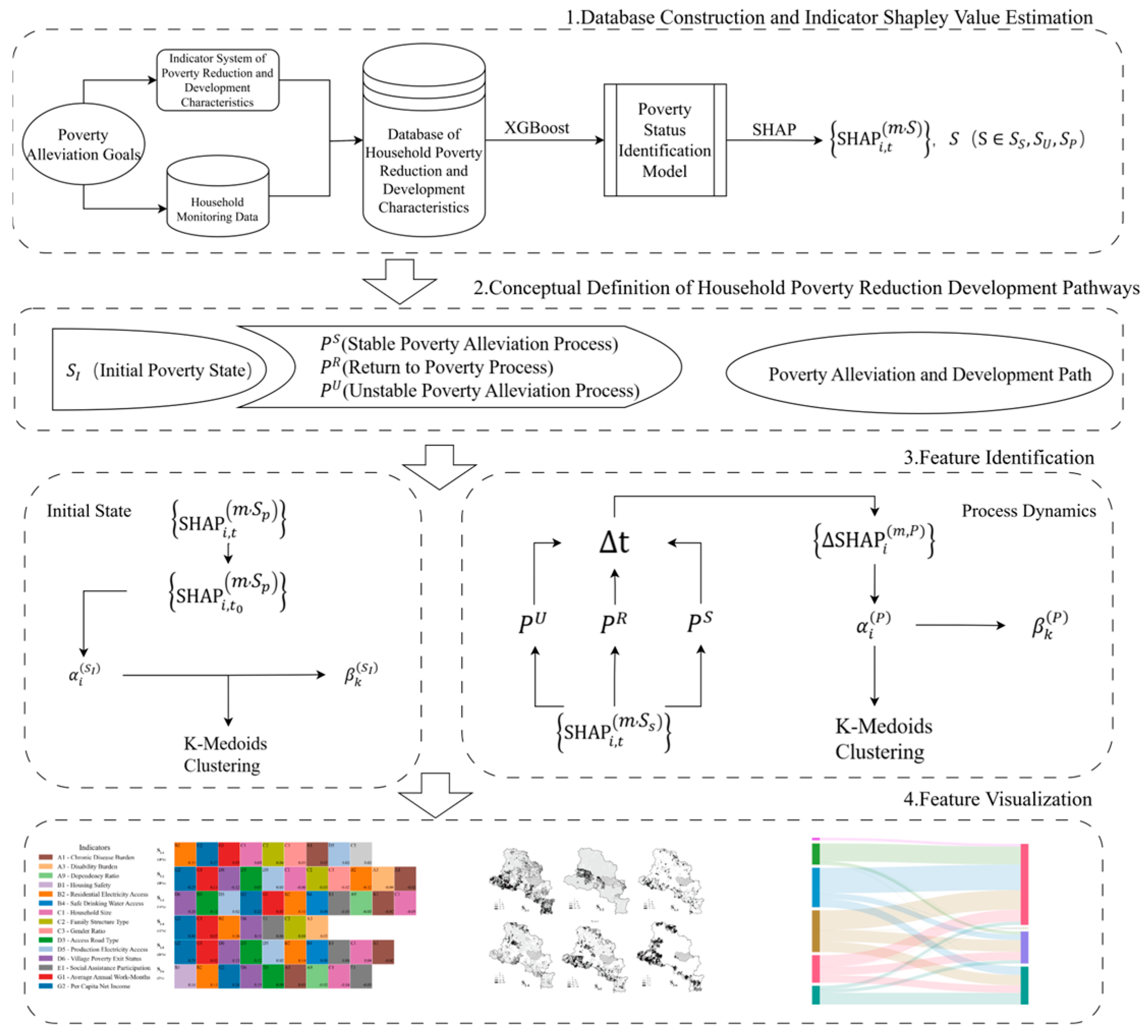
To effectively identify the characteristics of household poverty alleviation and development paths, this study introduces the Rural Household Poverty Alleviation and Development Path Identification Framework (Figure 2). Building on the strengths of the SHAP (Shapley Additive Explanations) method in providing interpretable insights, the framework utilizes multi-stage data processing, model training, and feature attribution analysis to uncover both the key influencing factors and the dynamic characteristics embedded in households′ poverty reduction and development paths. The framework consists of four key components. First, it involves constructing the database and calculating SHAP-based indicator indices. Second, it focuses on identifying the initial household states. Third, it includes recognizing the poverty reduction processes. Finally, it integrates state identification and process recognition to perform a comprehensive analysis of path features, thereby revealing the full structure of household poverty reduction and development paths.

2.4.1. Database Construction and SHAP Value Estimation of Indicators

Based on the proposed indicator system for household poverty alleviation and development paths, the original monitoring data were first cleaned and preprocessed. This stage involved handling missing values, removing outliers, and normalizing variables, which together resulted in the creation of the Feature Database. Missing values were handled through listwise deletion to maintain data integrity. Outliers in numerical variables (e.g., income) were treated using winsorization at the 1st and 99th percentiles. All continuous numerical variables (e.g., income) were standardized to a mean of 0 and standard deviation of 1 to mitigate the influence of varying scales.
Building on this foundation, we employed the XGBoost algorithm for multi-class classification of household poverty states. To benchmark its performance, we also implemented Random Forest and Decision Tree classifiers using scikit-learn. The hyperparameters for all models were optimized through an iterative process of manual tuning combined with cross-validation, aimed at maximizing the macro-average AUC. Hyperparameters were tuned via stratified cross-validation with early stopping, using Macro-F1 on validation folds for model selection; complete configurations and search ranges for XGBoost, Random Forest, and Decision Tree are reported in Appendix A Table A2. A comparative analysis of all models′ performance is provided in Section 3.1.
Feature attributions were then obtained from the optimized XGBoost model using the SHAP TreeExplainer with feature_perturbation = “interventional” to calculate exact SHAP values, capturing both the magnitude and direction of each feature′s contribution. In this study, each household is assessed annually and assigned to one of three possible states: S (where S S S , S U , S P ). For a given household m in year t, we obtain three sets of SHAP values for each indicator, denoted as S H A P i , t ( m , S ) . These values reflect the relative contribution of individual indicators to the classification of each state, thereby providing a quantitative foundation for subsequent feature identification and clustering analysis.

2.4.2. Identification of Initial State Characteristics

The initial state S I represents the point at which rural households are first incorporated into the monitoring and assistance system. The poverty characteristics observed at this stage determine the type of policy interventions that households may receive, and they also play a decisive role in shaping subsequent outcomes and the trajectory toward stable poverty alleviation.
For the purpose of initial-state identification, this study focuses on the poverty-class state ( S P ). Specifically, for household m at the initial time point t 0 , we select the corresponding SHAP value vector S H A P i , t 0 ( m , S p ) . This set of values provides the quantitative basis for identifying and analyzing the key characteristics of households’ starting poverty conditions, which in turn supports the subsequent recognition of development paths.
First, for each indicator, we calculate the Indicator SHAP Influence Coefficient α i ( S I ) under the initial state. This coefficient is obtained by normalizing the absolute SHAP values while retaining their original signs, thereby ensuring that the direction of influence is consistent with the sign of the SHAP attribution. The formula is expressed as follows:
α i S I = S H A P i S P j = 1 n   S H A P j S P , i   = 1,2 , , n
where S H A P i S P denotes the SHAP value of the i -th indicator under the poverty state S P , and n is the total number of indicators. This formulation normalizes the SHAP values across all indicators, thereby quantifying the relative influence of each indicator on the model’s classification of household states, while preserving the directional information encoded in the sign. A positive coefficient indicates that the indicator tends to classify the household as being in poverty, reflecting poverty-specific characteristics, whereas a negative coefficient suggests that the indicator is associated with poverty alleviation, highlighting a trend toward development.
Subsequently, we compute the Dimension-level SHAP Influence Coefficient β k S I for each dimension. For a given dimension k , the coefficient is defined as the sum of the absolute values of the indicator-level influence coefficients within that dimension:
β k S I = i D k   α i S I , k   = 1,2 , , K
where D k denotes the set of indicators belonging to dimension k , and K represents the total number of dimensions. This coefficient effectively captures the relative importance of each dimension in the identification of initial-state poverty characteristics.
After obtaining the indicator influence coefficients α i ( S I ) at the initial state, we applied the K-Medoids clustering algorithm to group the household samples. K-Medoids is a widely used unsupervised learning method that is particularly suitable for high-dimensional datasets containing multiple features. The cluster medoids derived from the algorithm represent the typical poverty characteristics of households within each group. To determine the optimal number of clusters, we employed a combination of the Elbow Plot and the Silhouette Coefficient, complemented by domain knowledge, to ensure a robust and substantively meaningful clustering solution. To further assess robustness, we conducted bootstrap resampling and calculated the Adjusted Rand Index (ARI), which confirmed the consistency of cluster assignments.
Finally, we applied a cumulative selection rule by ranking the absolute values of the indicator influence coefficients in descending order and retaining indicators until the cumulative contribution reached 0.9. For each cluster medoid, we then ranked the dimensions according to their dimension-level influence coefficients, and further ordered the indicators within each dimension by the absolute values of their indicator-level coefficients. Based on these rankings, we constructed heatmaps to visualize the differences in initial-state poverty characteristics across household categories and dimensions. In combination with spatial visualization, this approach allows for a more comprehensive analysis of the spatial distribution of households with distinct initial poverty profiles.

2.4.3. Identification of Process Dynamics Feature

Poverty reduction and development paths primarily reflect the dynamic transitions that households undergo across multiple stages in the pursuit of stable poverty alleviation. To analyze these processes, this study relies on the set of SHAP values corresponding to the stable poverty alleviation state S S , denoted as S H A P i , t ( m , S S ) , which serves as the data foundation for process-level identification. For each household, the complete path is first divided into distinct process stages, with both the starting and ending time points of each stage clearly defined. We then calculate the change in SHAP values for each indicator between the beginning and end of a given process, expressed as Δ S H A P i ( m , P ) . This change measures the variation in the relative contribution of indicator i during process P . A positive change indicates that the indicator facilitates the household’s transition toward stable poverty alleviation, whereas a negative change reflects an inhibiting effect that heightens the risk of falling back into poverty. Such differential analysis highlights the increasing or decreasing influence of key features along the evolution of poverty reduction and development paths, thereby providing interpretable evidence to support the examination of dynamic processes across different path types.
To facilitate both cross-sectional comparison and longitudinal trend analysis, we further calculated the indicator-level SHAP influence coefficients α i ( P ) and the dimension-level SHAP influence coefficients β k ( P ) , following the same procedure used in the identification of initial-state features. A larger α i ( P ) indicates that indicator i plays a more critical role in supporting households’ transition toward stable poverty alleviation during the corresponding stage, whereas a smaller or negative value implies a constraining effect. In parallel, β k ( P ) captures the dominant role of dimension k within that process stage, thereby providing a clearer understanding of how different dimensions contribute to the evolution of household poverty reduction and development paths.
Based on the indicator-level influence coefficients α i ( P ) , we applied the K-Medoids clustering algorithm to classify the process-level changes. The number of clusters was determined through a combined assessment using the Elbow Plot, the Silhouette Coefficient, and expert domain knowledge. Following the same ranking principles as in the initial-state analysis, we ordered the dimensions according to their aggregated influence coefficients and then ranked the indicators within each dimension by the magnitude of their α i ( P ) . On this basis, we constructed heatmaps to visualize the characteristic differences across process categories and further mapped their spatial distributions. This procedure enables a clear identification of how key dimensions and indicators vary dynamically during different poverty reduction and development processes, while also providing insights into the spatial patterns of diverse household trajectories.

2.4.4. Recognition and Analysis of Poverty Reduction and Development Path Features

By combining the results of initial-state feature identification with the analysis of process-level dynamics, this study obtains complementary information on the key characteristics of households at both the starting point and during subsequent transitions. Integrating these two sources of information enables us to systematically capture the full set of feature patterns that characterize the evolution from the initial poverty state through all intermediate processes to the attainment of stable poverty alleviation. This comprehensive recognition of poverty reduction and development path features not only provides a holistic understanding of the dynamic mechanism of household poverty alleviation, but also establishes a solid foundation for subsequent path classification and the design of differentiated policy measures.
To provide an intuitive representation of path transitions, this study employs the Sankey Diagram as the primary visualization tool to depict the flows and proportions of transitions across different states. On the left side of the diagram, the initial state categories of households at the time of their inclusion in the poverty reduction monitoring system are displayed, while the subsequent process types are shown sequentially from left to right. The width of each flow line directly reflects the magnitude of transitions between categories, thereby revealing the dominant trends through which households move from their initial states into different processes. Building on this overall visualization of transition patterns, we further select several representative paths and conduct spatial distribution analyses. This approach allows for a more detailed deconstruction of household poverty reduction and development path features, as well as a deeper understanding of their spatial differentiation.

3. Results

3.1. Overall Characteristics of Key Indicators Across the Three States

The household poverty reduction and development state classification model was developed using the XGBoost algorithm, which demonstrated superior performance (macro-average AUC = 0.97) compared to Random Forest (0.95) and Decision Tree (0.91) benchmarks. The model exhibited strong performance in distinguishing among the three states. Specifically, the area under the ROC curve (AUC) for the poverty state ( S P ) is 0.99, indicating highly precise identification. The stable poverty alleviation state ( S S ) and the unstable poverty alleviation state ( S U ) achieved AUC values of 0.96 and 0.94, respectively. Although slightly lower, these values still reflect robust classification performance. The identification of absolute poverty is based on a well-defined national poverty standard, which provides clear and consistent criteria. In contrast, the classification of stable and unstable poverty alleviation states depends more heavily on the subjective judgment and practical experience of local officials and field workers, which increases similarity between these two categories in the feature space. Nevertheless, the model maintains high recognition accuracy across all states, enabling us to reliably map states and processes that are directly relevant to sustainable poverty alleviation.
Building on this validated performance, we further employed the SHAP method to examine feature importance. Figure 3 presents the ten most influential indicators for each state, along with the distribution of SHAP values and the corresponding effects of different feature values. Specifically, the upper X-axis in each figure denotes the absolute mean SHAP contribution of each indicator across all samples, while the lower X-axis illustrates the distribution of SHAP values associated with different feature levels. This visualization highlights both the relative importance of indicators under different states and the directional nature of their contributions, providing an intuitive understanding of the feature differences that characterize poverty reduction and development states and how these differences underpin (un)sustainable trajectories.
In the poverty state ( S P ), access to safe drinking water (B4) emerges as a distinctive indicator relative to the stable ( S S ) and unstable ( S U ) poverty alleviation states. Regarding the distribution of SHAP values, both per capita net income (G2) and residential electricity access (B2) display wide variation in both positive and negative directions. Indicators such as social assistance participation (E1), household size (C1), and village poverty exit status (D6) show broadly positive SHAP distributions, whereas household size (C1) and access road type (D3) exhibit stronger negative contributions. For most indicators, SHAP values change monotonically with feature levels, but disability burden (A3) and access road type (D3) present more complex, non-monotonic patterns. Overall, the classification of poverty states relies primarily on clearly defined indicators linked to basic living burdens (Category A), emphasizing fundamental livelihood needs whose remediation constitutes the necessary baseline for any sustainable poverty alleviation.
In the unstable poverty alleviation state ( S U ), several policy-related support indicators are uniquely important, including photovoltaic project participation (E3), agro-processing assistance (F2), and the dilapidated housing renovation project (B3). In terms of SHAP value distributions, the allowance for needy families (E1) shows wide variation in both directions. Public welfare employment participation (E2), photovoltaic project participation (E3), and household size (C1) display higher contributions on the positive side, whereas residential electricity access (B2), per capita net income (G2), and access road type (D3) show stronger negative contributions. Notably, indicators such as public welfare employment participation (E2), allowance for needy families (E1), agro-processing assistance (F2), household size (C1), and the dilapidated housing renovation project (B3) exhibit complex and heterogeneous relationships with SHAP values. To promote stable poverty alleviation among households in the unstable poverty reduction state, the provision of public welfare employment opportunities and industrial support during periods of unstable development or insecure income sources provides the necessary buffer conditions that bridge unstable conditions toward sustainable poverty alleviation, especially when livelihoods are intermittently insecure.
In the stable poverty alleviation state ( S S ), distinctive indicators include production electricity access (D5), gender ratio (C3), and the education level of the labor force (C5). The access road type (D3) rises sharply in importance, ranking highest with a broad positive contribution range. Meanwhile, per capita net income (G2) shows wide variation in both positive and negative directions, while residential electricity access (B2) exhibits more extensive negative distributions. Moreover, indicators such as disability burden (A3), public welfare employment participation (E2), and gender ratio (C3) display diverse and non-linear contribution trends as their feature values increase. The determination of the stable poverty alleviation state is shaped mainly by indicators of the production environment (Category D) and human capital (Category C), suggesting that strengthening both human resources and production conditions is essential to secure lasting and sustainable poverty alleviation outcomes by enhancing household resilience to shocks.
Overall, per capita net income (G2), residential electricity access (B2), access road type (D3), and village poverty exit status (D6) consistently rank among the top ten indicators across all three states in terms of SHAP values. From the perspective of indicator composition, as households transition from the poverty state toward the stable poverty alleviation state, the top ten indicators shift in emphasis—from those primarily reflecting housing facilities and living burdens to those highlighting development-support measures and production resources.

3.2. Identification of Initial State and Dynamic Process Features

The optimal cluster numbers for the initial state and the three poverty alleviation processes were determined by jointly considering the Elbow Plot, the Silhouette Coefficient, and the interpretability of the results. The analysis identified six clusters for the initial state, seven for the stable poverty alleviation process, three for the return-to-poverty process, and four for the unstable poverty alleviation process.
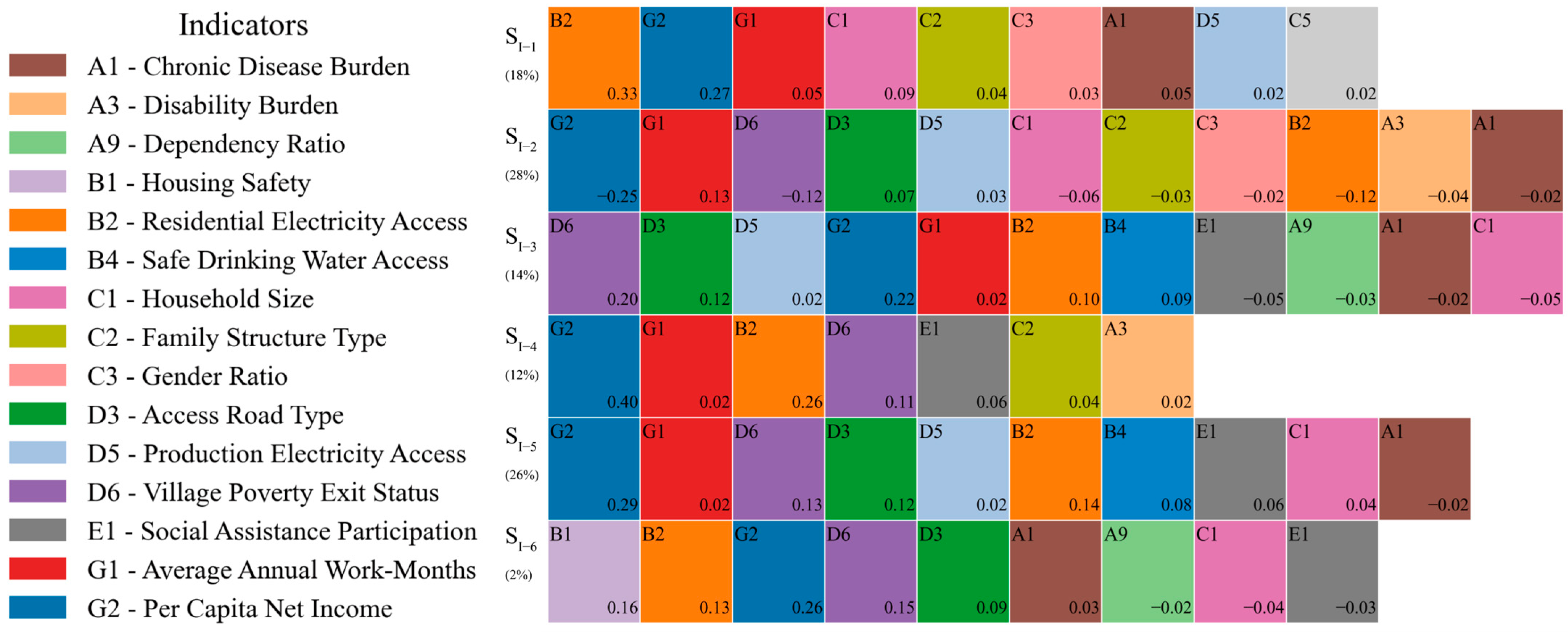
As shown in Figure 4 and Figure 5, the cluster centers of the initial state and their spatial distributions are presented. In the heatmaps, positive SHAP values indicate features contributing to the classification of households as being in the poverty state ( S p ), whereas negative values represent advantageous features that facilitate poverty alleviation and signal higher potential for sustainability if maintained or strengthened.
Regarding group size, S I 2 and S I 5 account for the largest shares, at 28% and 26% respectively, while S I 6 represents the smallest cluster. In terms of overall feature differences, S I 2 is clearly distinct from the others: most of its indicator influence coefficients are negative, suggesting relative advantages in poverty alleviation, although it is still identified as part of the unstable poverty alleviation state. The key poverty-related features of this cluster are primarily associated with G1: Average Annual Work-Months and D3: Access Road Type.
For the remaining clusters, the most influential features are concentrated in the Housing & Infrastructure dimension (B2: Residential Electricity Access, B4: Safe Drinking Water Access), the Production Resources dimension (D5: Production Electricity Access, D6: Village Poverty Exit Status), and the Labor & Income dimension (G1: Average Annual Work-Months, G2: Per Capita Net Income). More specifically:
  • S I 1 shows pronounced poverty-related characteristics in the Human Capital dimension (C1: Household Size, C2: Family Structure Type).
  • S I 3 demonstrates relative advantages within the Social Protection Measures dimension (E1: Allowance for Needy Families) and several indicators of the Living Burdens dimension (A1: Chronic Disease Burden, A9: Dependency Ratio), yet still exhibits a poverty-related feature in B4: Safe Drinking Water Access (Housing & Infrastructure).
  • S I 4 and S I 5 are both strongly associated with E1: Allowance for Needy Families (Social Protection Measures). However, S I 4 shows additional poverty-related characteristics in C2: Family Structure Type (Human Capital) and A3: Disability Burden (Living Burdens), whereas S I 5 is characterized by poverty in C1: Household Size (Human Capital) and B4: Safe Drinking Water Access (Housing & Infrastructure), but displays an alleviation advantage in A1: Chronic Disease Burden (Living Burdens).
  • S I 6 exhibits advantages across multiple dimensions, yet still shows a relatively high poverty-related feature in B1: Housing Safety (Housing & Infrastructure).
From a spatial perspective, households in all clusters are predominantly concentrated in mountainous and resource-dependent areas. Within this distribution, S I 1 and S I 4 are more prevalent in regions with abundant arable land resources, while S I 3 , S I 5 , and S I 6 exhibit more spatially clustered patterns.
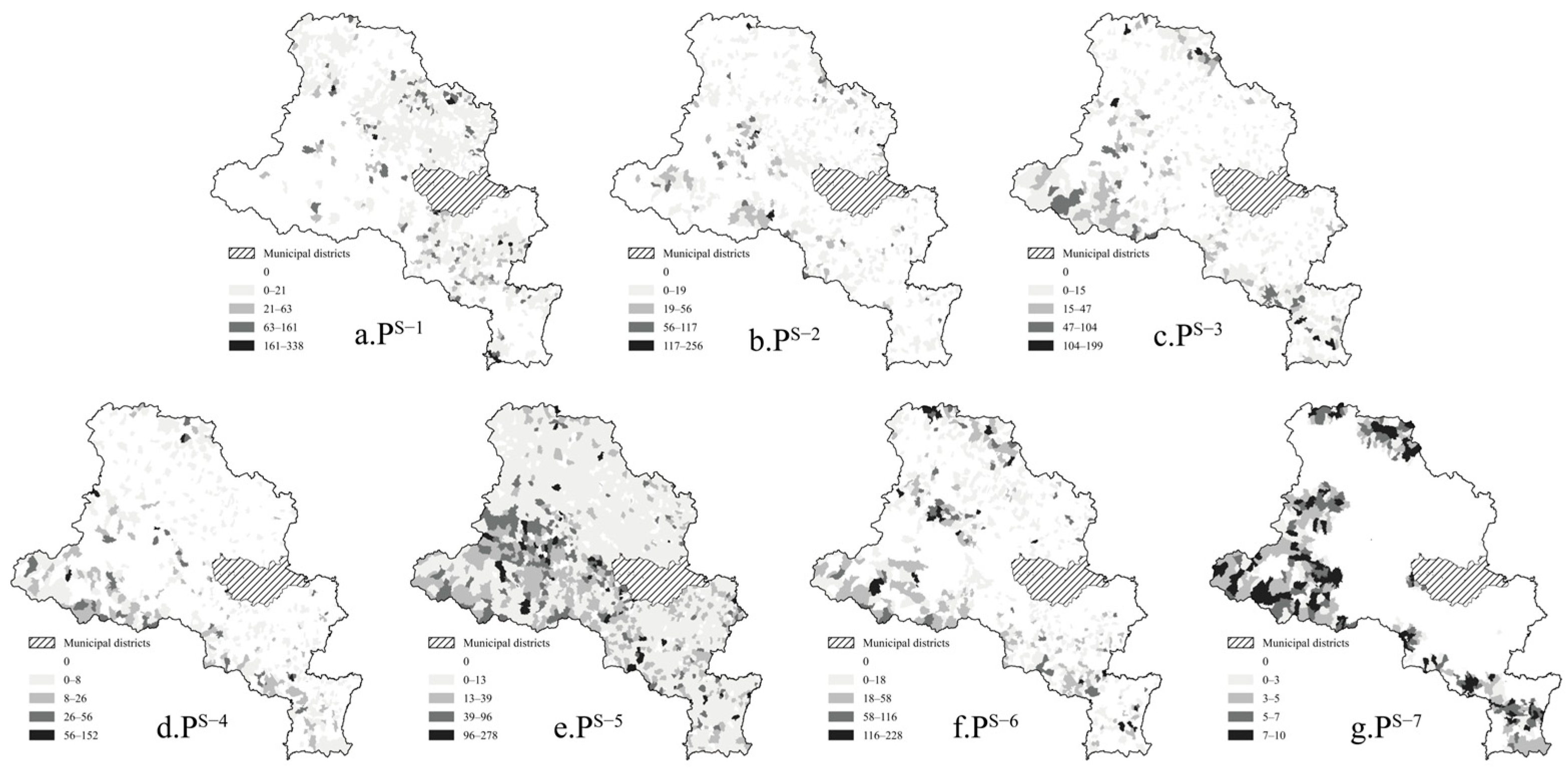
As shown in Figure 6 and Figure 7, the cluster centers of the stable poverty alleviation process ( P S ) and their spatial distributions are illustrated. In terms of group size, P S 1 (20%), P S 5 (38%), and P S 6 (18%) constitute the major pathways through which households achieve stable poverty alleviation. Regarding feature dynamics, all cluster centers exhibit positive changes in their dominant dimensions. Among them, P S 2 , P S 3 , P S 4 ,and P S 7 are primarily characterized by improvements in the Production Resources dimension (Category D), while P S 1 , P S 5 , and P S 6 display more significant changes in the Labor & Income dimension (Category G). With respect to specific indicator composition:
  • P S 1 shows marked changes in D1: Cultivated Land Area (Production Resources), C1: Household Size (Human Capital), and C2: Family Structure Type (Human Capital).
  • Both P S 2 and P S 4 exhibit positive changes in D2: Other Agricultural Land Area (Production Resources), indicating that households in these clusters primarily rely on diversified farmland resources—such as forestry, orchards, and aquaculture—for achieving stable poverty alleviation. Beyond this common foundation, their feature dynamics diverge: P S 2 is mainly characterized by improvements in F2: Agro-processing Assistance (Industry-Assisted Measures), C1: Household Size (Human Capital), and C3: Gender Ratio (Human Capital), whereas P S 4 shows positive changes in D5: Production Electricity Access (Production Resources), C6: Skilled Labor Share (Human Capital), and C8: Participation in Education Aid Programs (Human Capital).
  • P S 3 is characterized by improvements in D4: Distance to Main Village Road (Production Resources), D6: Village Poverty Exit Status (Production Resources), G2: Per Capita Net Income (Labor & Income), and C2: Family Structure Type (Human Capital).
  • P S 5 is more strongly associated with positive changes in G2: Per Capita Net Income (Labor & Income), G1: Average Annual Work-Months (Labor & Income), and C2: Family Structure Type (Human Capital).
  • Both P S 6 and P S 7 exhibit substantial positive changes in the Social Protection Measures dimension (Category E), underscoring the importance of policy-driven support in sustaining poverty alleviation. Their specific feature dynamics, however, differ: P S 6 is characterized by improvements in E1: Allowance for Needy Families and E2: Public Welfare Employment Participation, accompanied by gains in G2: Per Capita Net Income (Labor & Income), whereas P S 7 is distinguished by notable changes in E3: Photovoltaic Project Participation and E4: Ecological Compensation Participation, along with a significant improvement in B1: Housing Safety (Housing & Infrastructure). This comparison suggests that while both clusters rely heavily on social protection programs, P S 6 reflects a pathway centered on livelihood security through cash and employment support, whereas P S 7 highlights ecological and infrastructural interventions as key drivers of stable poverty alleviation with co-benefits for sustainable development.
From a spatial perspective, households in P S 1 to P S 4 are relatively more concentrated in areas with abundant arable land resources or within the plains, compared with other clusters, whereas the distributions of P S 5 to P S 7 broadly correspond to the overall settlement pattern of poor households in the study area.
Figure 6. Heatmap of Cluster Centers in the Stable Poverty Alleviation Process.
Sustainability 17 09704 g006
Figure 7. Spatial Distribution of Clustering Results in the Stable Poverty Alleviation Process.
Sustainability 17 09704 g007
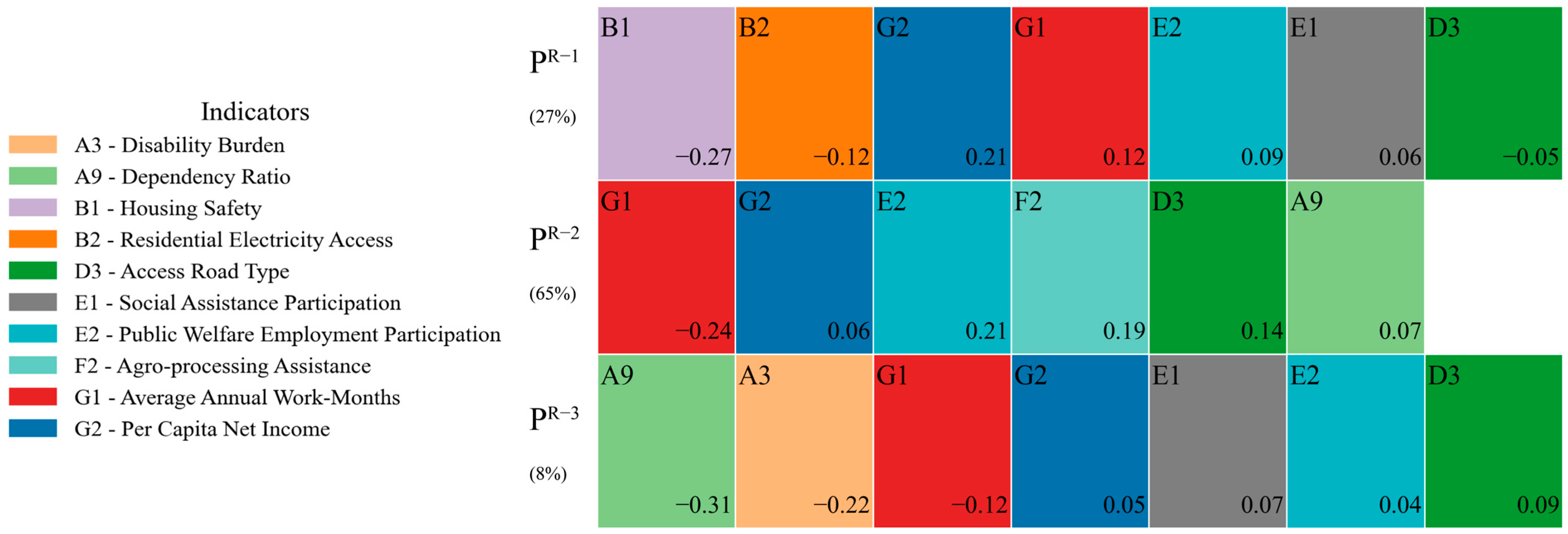
As shown in Figure 8 and Figure 9, the cluster centers of the return-to-poverty process ( P R ) and their spatial distributions are illustrated. Overall, households experiencing re-poverty are primarily associated with disadvantages in the Living Burdens dimension (Category A), the Labor & Income dimension (Category G), and the Housing & Infrastructure dimension (Category B). Among these, P R 2 is the dominant type, accounting for 65% of the households undergoing this process.
In terms of structural characteristics, P R 1 is mainly characterized by vulnerabilities in housing and infrastructure conditions, particularly B2: Residential Electricity Access, B1: Housing Safety, and D3: Access Road Type. The re-poverty features of P R 2 are reflected in strong fluctuations in employment and income indicators, namely G1: Average Annual Work-Months and G2: Per Capita Net Income. By contrast, P R 3 is closely associated with disadvantages in living burdens, especially A3: Disability Burden.
From a spatial perspective, households in P R 1 are relatively more concentrated in mountainous and hilly areas, whereas those in P R 2 and P R 3 are more dispersed across the study area. The results suggest that re-poverty risks exhibit pronounced spatial patterns in relation to housing and infrastructure conditions, whereas the spatial differentiation of other livelihood-related factors is relatively weak.
As shown in Figure 10 and Figure 11, the cluster centers of the unstable poverty alleviation process ( P U ) and their spatial distributions are presented. Overall, with the exception of P U 3 , most cluster centers are dominated by positive changes in indicators from the Production Resources dimension (Category D) and the Labor & Income dimension (Category G). In contrast, P U 3 is mainly characterized by re-poverty features associated with increases in the Living Burdens dimension (Category A, e.g., A1: Chronic Disease Burden; A3: Disability Burden) and reductions in G1: Average Annual Work-Months (Labor & Income).
In terms of structural differences, P U 1 and P U 2 are distinguished by the positive role of Social Protection Measures (Category E) combined with improvements in the Living Burdens dimension (Category A) in facilitating transitions toward stable poverty alleviation. Specifically, P U 1 is characterized by contributions from E2: Public Welfare Employment Participation together with improvements in disease-related burdens (A1: Chronic Disease Burden; A3: Disability Burden), whereas P U 2 is more strongly associated with E4: Ecological Compensation Participation, alongside contributions from G2: Per Capita Net Income and G1: Average Annual Work-Months. By contrast, P U 4 highlights improvements in the Human Capital dimension (Category C), particularly C2: Family Structure Type and C8: Participation in Education Aid Programs, reflecting enhanced labor quality and educational support. Among the P U types, P U 1 and P U 2 serve as policy-enabled transitions toward sustainability, whereas P U 3 flags medical and dependency burdens that erode sustainability unless addressed.
From a spatial perspective, households in P U 2 and P U 4 are relatively more concentrated in mountainous and hilly regions, whereas those in P U 1 and P U 3 are more scattered, indicating stronger spatial heterogeneity in unstable poverty alleviation pathways.

3.3. Identification of Poverty Alleviation and Development Path Features

The clustering results of the initial state ( S I ) and different process types ( P S , P R , P U ) reveal the key characteristics and categorical differences in households’ poverty alleviation and development. However, feature extraction based on a single state or a single process is insufficient to fully uncover the underlying mechanisms of the complete trajectory. Instead, households’ poverty alleviation and development paths are composed of dynamic combinations of multiple states and processes, exhibiting distinct stage-specific patterns and household-level heterogeneity. Therefore, building on the preceding identification results, this section integrates households’ initial states and dynamic processes, constructs path representations and typologies, and identifies characteristic patterns of path variation.
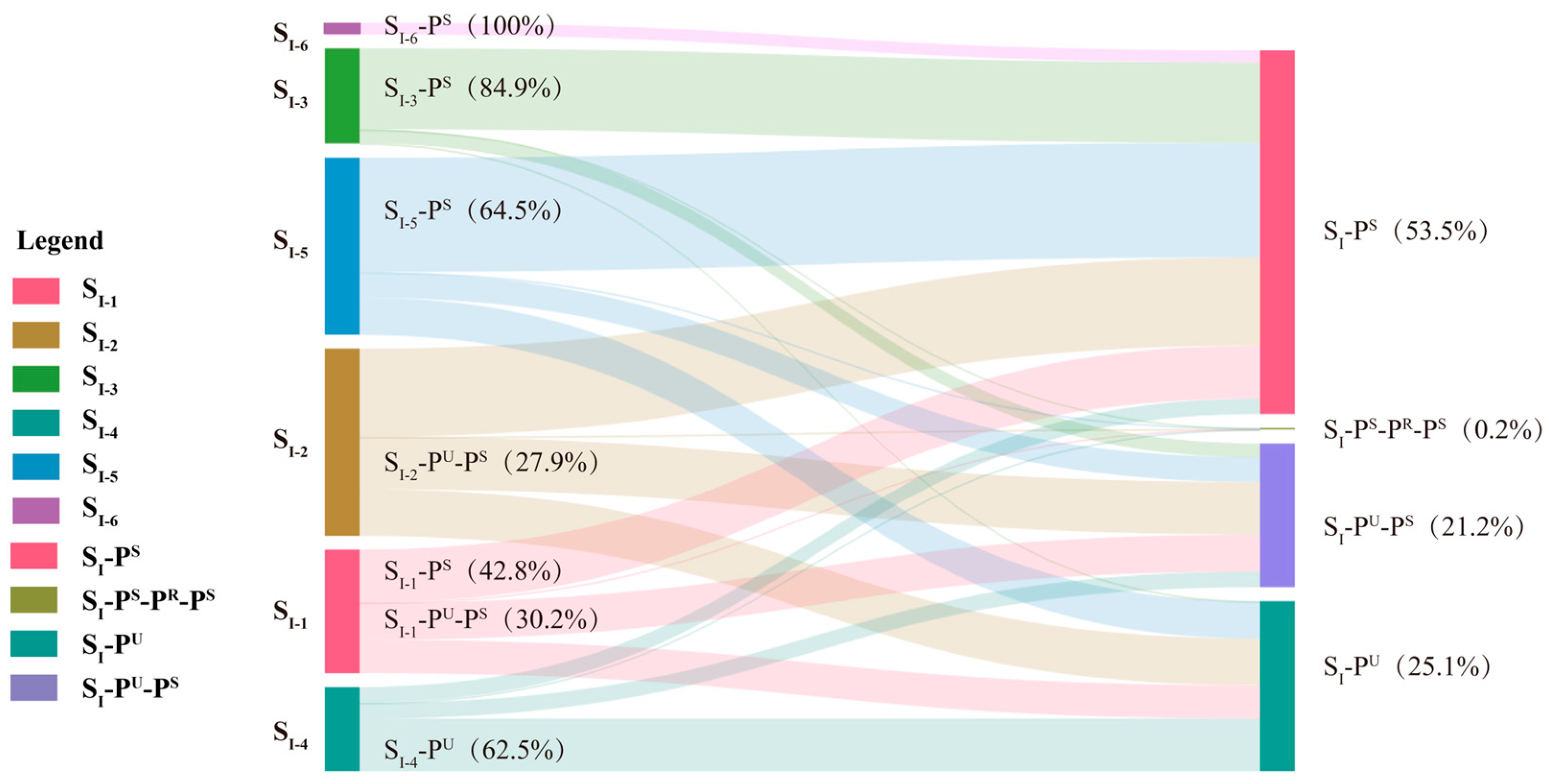
Figure 12 illustrates the overall distribution of different household poverty reduction and development path types. In general, the trajectories can be classified into four categories: S I P S (53.5%), S I P U (25.1%), S I P U P S (21.2%), and S I P S P R P S (0.2%). Examining the preferences across different initial states, the S I P S path type is most prevalent among households in S I 6 (100%), S I 3 (84.9%), S I 5 (64.5%), and S I 1 (42.8%), indicating a greater tendency for these groups to achieve stable poverty alleviation directly. In the S I P U P S category, households in S I 1 (30.2%) and S I 2 (27.9%) account for the largest shares, suggesting that these groups tend to pass through an unstable poverty alleviation stage before attaining stability. By contrast, within the S I P U type, S I 4 represents the dominant group (62.5%), which remains in an unstable poverty alleviation state at present.
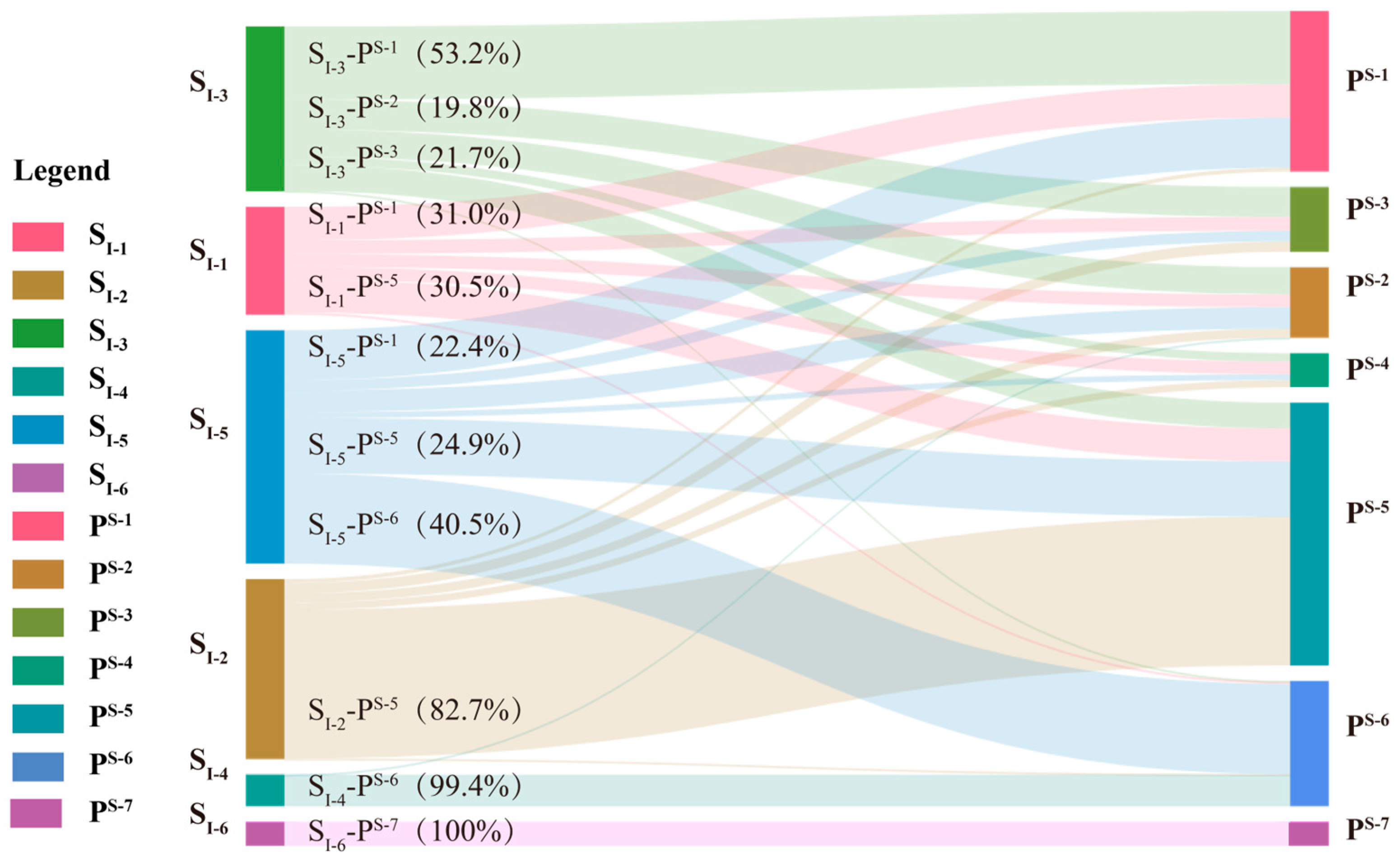
Figure 13 illustrates the variation within the S I P S path type. In terms of distribution across P S subcategories, P S 5 accounts for the largest share (35.4%), followed by P S 1 (21.6%) and P S 6 (16.9%). Across different initial states, households in S I 2 , S I 4 , and S I 6 tend to rely on a single P S subtype to achieve stable poverty alleviation, whereas those in S I 1 , S I 3 , and S I 5 display more diversified pathways toward stability. The predominance of P S 5 and P S 1 within S I P S indicates that stable income and capability accumulation are central to sustainable exits.
Figure 14 illustrates the variation relationships within the S I P U and S I P U P S path types. Regarding the correspondence from the initial state to the unstable poverty alleviation process, 88.5% of S I 4 households transition into P U 1 , while the majority of S I 5 (68.9%) transition into P U 2 . Most households in S I 2 (89.6%) and S I 3 (93.9%) are associated with P U 4 , whereas S I 1 is more evenly distributed between P U 2 (38.8%) and P U 4 (43.7%). In terms of transitions from the unstable poverty alleviation process to the stable poverty alleviation process, both P U 3 and P U 4 primarily shift to P S 5 (51.3% and 57.8%, respectively) and P S 1 (22.3% and 13.0%). P U 1 is predominantly linked to P S 6 (85.7%). By contrast, P U 2 shows a more diverse transition pattern, with 32.7% shifting to P S 6 , 26.0% to P S 1 , and 21.3% to P S 5 . Overall, the preferences of different initial states in selecting P S categories for achieving stable poverty alleviation are broadly consistent with the patterns observed in the direct S I P S pathways. Transitions from P U 1 , P U 2 , and P U 4 into P S 5 , P S 1 , and P S 6 reveal concrete bridging routes to sustainability, while P U 3 requires burden-reduction policies to avoid relapse.
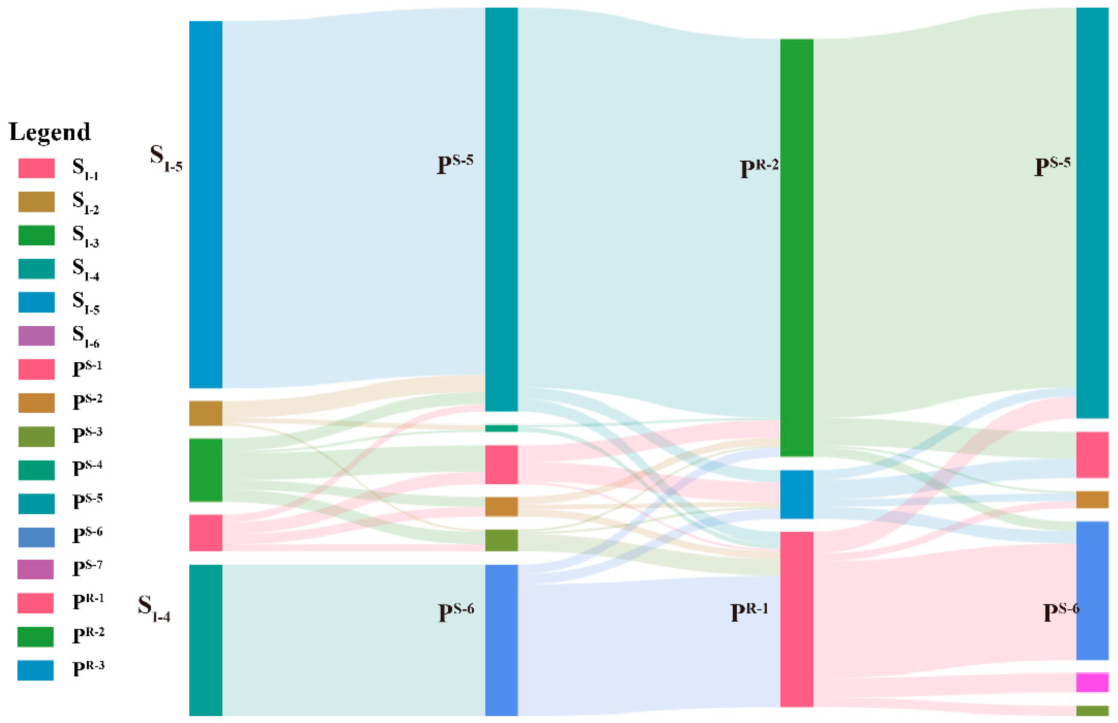
Within the S I P S P R P S path type (Figure 15), a total of 264 households were identified. Among them, S I 5 P S 5 P R 2 P S 5 constitutes the largest group (57%), followed by S I 4 P S 6 P R 1 P S 6 (18%), which together represent the dominant patterns of this trajectory. In terms of structural characteristics, a notable feature of this path type is that the two P S subcategories at the beginning and end remain identical, indicating a relatively stable configuration of poverty alleviation processes and suggesting that re-establishing the same P^S subtype can effectively reconsolidate sustainability after shocks.

3.4. Characteristics of Typical Poverty Alleviation and Development Paths

The formation of household poverty reduction and development paths is influenced by multiple factors, including initial characteristics, natural–social environments, and external policy and industrial conditions. Consequently, these paths show high complexity and heterogeneity. To capture their essential patterns, this section focuses on representative groups with significant features, analyzing their main path variations and spatial distribution characteristics.
The S I 4 and S I 5 groups, both identified at the initial state as households receiving minimum living allowances, exhibit markedly different outcomes in their subsequent poverty reduction and development paths. S I 4 forms the largest cluster still trapped in the unstable poverty alleviation process ( P U ), with 62.5% of households yet to achieve stability. In contrast, S I 5 demonstrates a relatively high level of stability, with 78.5% of households having successfully transitioned into the stable poverty alleviation state ( S s ). Among the remaining groups, S I 1 and S I 3 display pronounced differences in the Human Capital dimension (Category C), which are reflected in their divergent path outcomes: while 99.5% of households in S I 3 have achieved stable poverty alleviation, 27% of those in S I 1 remain in the unstable state. Accordingly, these four initial-state groups are selected as representative cases to contrast sustainability potentials, dependencies, and failure risks across pathways for further analysis of poverty reduction and development path features.
From the perspective of poverty reduction and development paths, both S I 4 (37%) and S I 5 (31.2%) primarily rely on the P S 6 pathway to achieve stable poverty alleviation. However, the S I 5 group also attains stability through more diversified routes, including P S 5 (19.3%), P S 1 (15.8%), and P S 2 (7.2%), reflecting a broader range of path choices. With regard to unstable poverty alleviation processes, 71.4% of S I 4 households transitioned through P U 1 , of which 16.6% ultimately reached stable poverty alleviation; in contrast, 24.1% of S I 5 households experienced P U 2 , with 9.6% eventually achieving stability. Overall, the S I 4 group depends heavily on policy-oriented measures such as public welfare employment (E2) and social assistance (E1), indicating a poverty reduction and development path that is strongly reliant on external support and therefore exhibits weaker sustainability due to limited endogenous capacity. By comparison, the S I 5 group, mainly located in mountainous areas (Figure 5), demonstrates relative advantages in human resources and is thus better positioned to integrate local resource endowments and achieve stable poverty alleviation through industry-driven development that strengthens endogenous resilience and long-term sustainability.
In terms of the pathways leading to stable poverty alleviation, S I 1 households are more likely to experience the P U process before achieving stability, with a relatively balanced distribution between S I 1 P S (42.8%) and S I 1 P U P S (30.2%). By contrast, S I 3 households predominantly achieve stability directly through S I P S (84.9%). Regarding the choice of P S subtypes, S I 1 mainly follows P S 1 (24.0%) and P S 5 (21.4%), whereas S I 3 relies more heavily on P S 1 (43.2%) and P S 5 (16.0%), with additional contributions from P S 2 (17.7%) and P S 3 (17.4%). In terms of livelihood strategies, crop cultivation and off-farm wage employment constitute the predominant options for most poor households. Benefiting from stronger human capital, however, S I 3 households are able to combine policy support with local resources to pursue more diversified development pathways. For P U subtype selection across initial states, S I 3 shows a preference for P U 4 (14.1%), while S I 1 is more inclined toward P U 2 (22.2%) and P U 4 (25.0%). Notably, the share of S I 1 P U 2 P S (10.8%) is substantially lower than that of S I 1 P U 4 P S (14.2%) and S I 3 P U 4 P S (13.7%), suggesting that improvements in labor skills play a more decisive role in promoting stable poverty alleviation and in converting fragile transitions into sustainable, non-relapse outcomes.
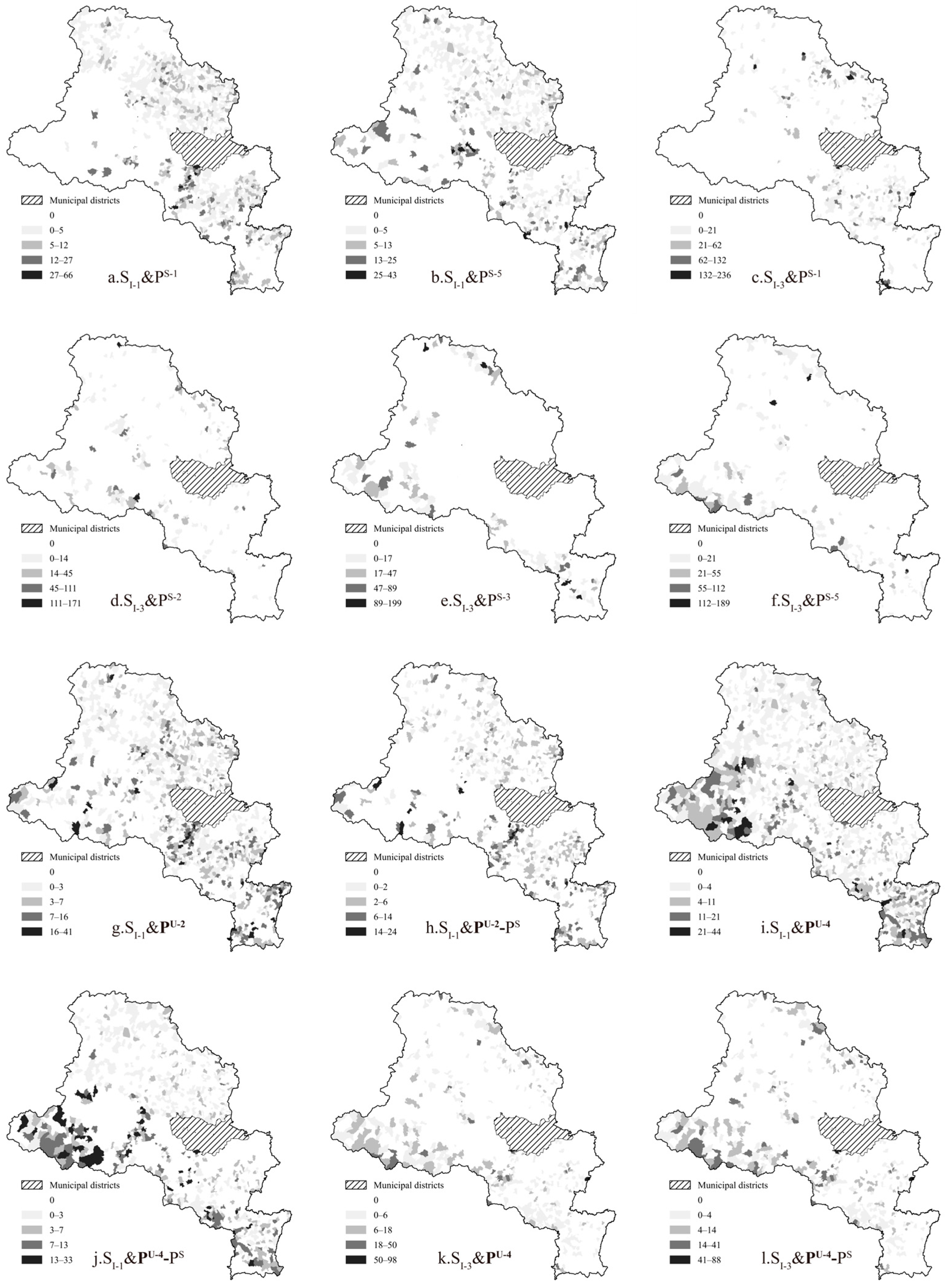
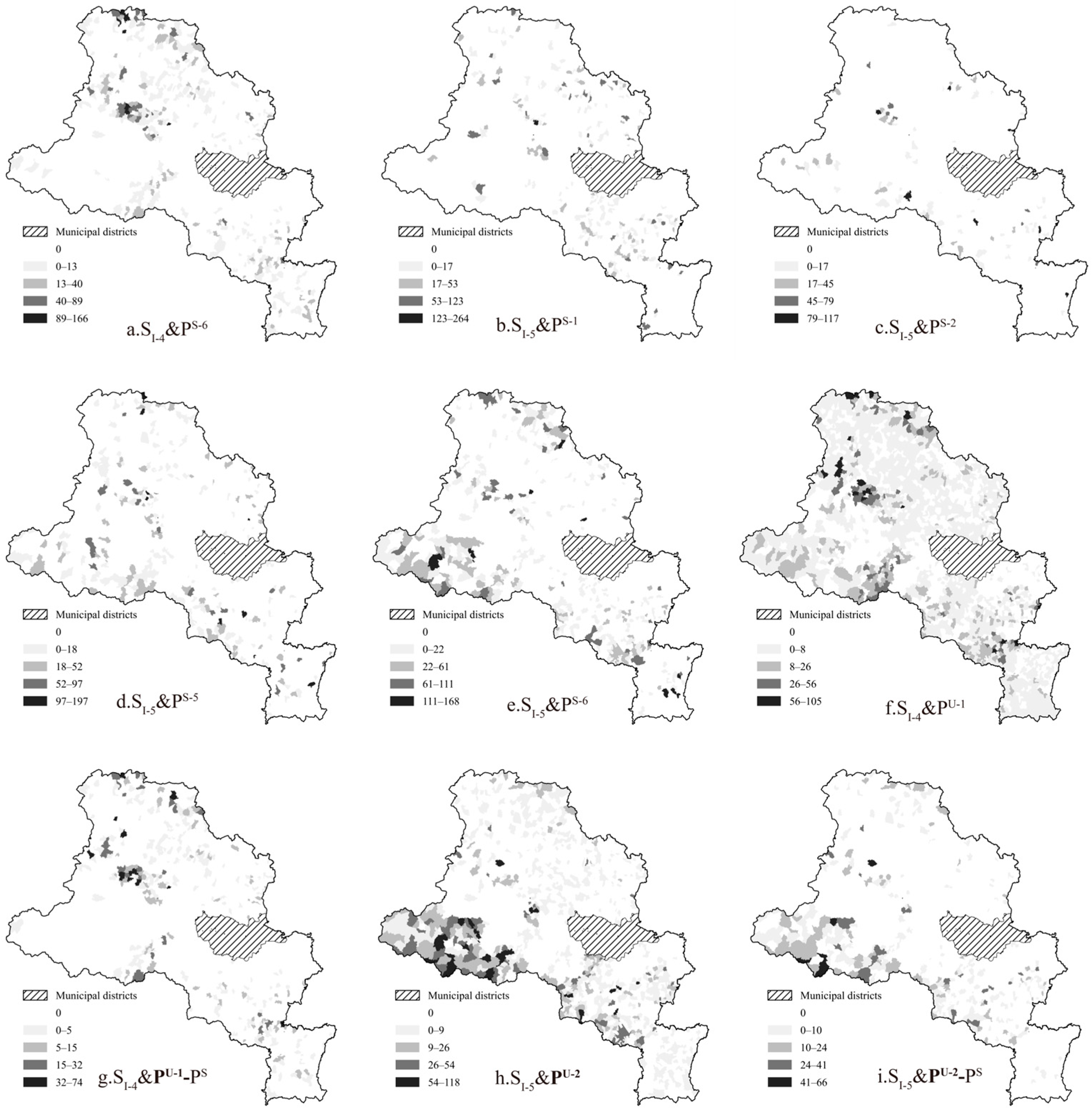
From the perspective of the spatial distribution of pathways to stable poverty alleviation across the four initial states (Figure 16 and Figure 17), P S 1 , P S 2 , P S 3 and P S 6 show similar spatial patterns despite differences in their realization rates among household types. In contrast, the spatial distribution of P S 5 exhibits a certain degree of randomness. Moreover, the distribution of rural livelihoods dominated by agriculture and sideline industries is largely shaped by regional resource endowments. The spatial distribution of households’ livelihood development pathways reflects the same pattern.
From the perspective of spatial differences in the number of pathways to stable poverty alleviation, S I 3 , S I 4 , and S I 5 generally exhibit more significant spatial clusters of high values across different pathways, whereas S I 1 shows relatively fewer. S I 3 and S I 5 , with relative advantages in human capital and lighter household burdens, often enable poor households within resource-rich villages and under policy support to achieve stable poverty alleviation through similar pathways. S I 4 , which achieves stable poverty alleviation mainly through P S 6 , relies heavily on government protective support policies and regional public welfare positions. In mining areas and ecological protection zones in particular, these regions provide more welfare positions and financial assistance, thereby generating higher numbers of households lifted out of poverty through this specific pathway. In contrast, S I 1 , which is more spatially dispersed, commonly faces serious human capital constraints. Since the conditions of these households largely fall outside the coverage of protective support policies and they lack competitiveness, their stable poverty alleviation is more often achieved through crop cultivation and off-farm wage employment. Spatial clusters where policy-led P S 6 dominates signal sustainability contingent on institutional support, whereas clusters with income-/capability-led P S 1 and P S 5 indicate stronger endogenous sustainability.

4. Discussion and Implications

4.1. Mechanisms of Pathways to Stable Poverty Alleviation

(1)
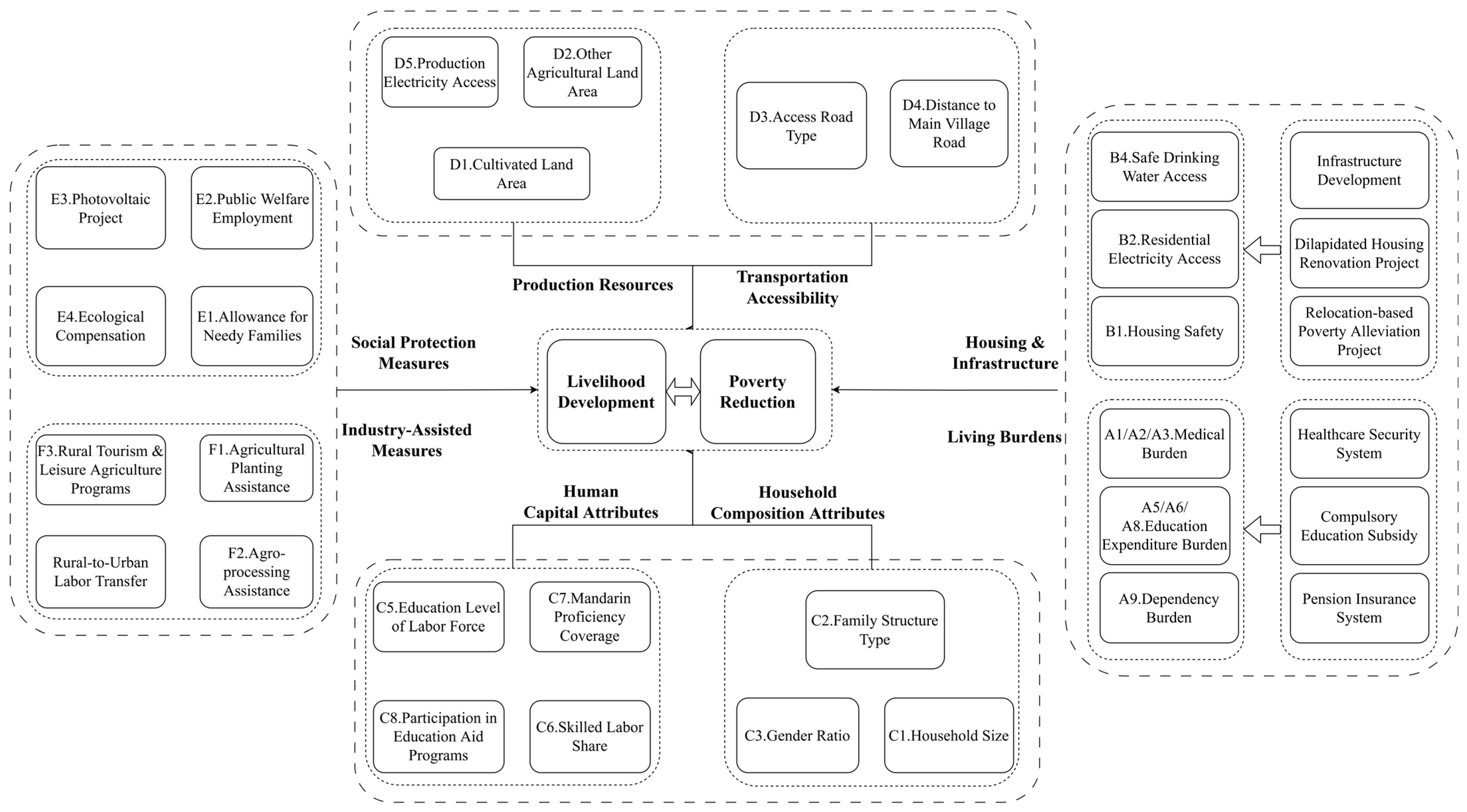
The process of achieving stable poverty alleviation consistently centers on the fundamental goal of eradicating poverty (Figure 18). Accurate identification of households’ initial poverty characteristics is a prerequisite for formulating effective policies and implementing targeted interventions. During China’s stage of Targeted Poverty Alleviation, the standard of poverty identification was established as the basic criterion for evaluating household poverty status [59,60]. This standard consisted of two major aspects: the minimum guarantee of basic living conditions, including food and essential daily necessities; and the assurance of access to fundamental public services, particularly in education, healthcare, and housing.
In terms of initial states, most households face two major constraints: deficits in Housing and Infrastructure and burdens in Living Burdens. Deficits in Housing and Infrastructure are mainly reflected in inadequate access to B4. Safe Drinking Water Access, B2. Residential Electricity Access, and B1. Housing Safety. With the implementation of the New Rural Construction Program, these problems have been effectively alleviated or largely resolved for many households [61,62], a pattern also reflected in Korea’s Saemaul Undong, where improvements in rural housing and infrastructure were closely linked with community mobilization to address structural disadvantages and promote sustainable development [63]. Nevertheless, some households ( S I 6 ) still rely on protective support measures—most notably relocation-based poverty alleviation projects and large-scale dilapidated housing renovation programs that targeted over 7.9 million rural households ( P S 7 )—to achieve stable poverty alleviation [64]. However, such reliance on relocation and large-scale housing renovation indicates a policy-dependent form of stability, raising questions about the long-term sustainability of these outcomes once intensive interventions are withdrawn. To secure long-term resilience for these households, subsequent efforts should integrate an asset-building approach into project designs. For instance, pairing housing improvements with skills training for home-based businesses or support for courtyard economies can help transform fixed assets into sustainable income-generating capabilities.
Living Burdens are primarily associated with medical, educational, and dependency-related pressures. Within this dimension, A5/A6/A8: Education Expenditure Burden and A2: Major Illness Burden are less dominant features of households’ initial poverty states, largely due to China’s nine-year compulsory education policy and catastrophic-illness insurance, which have substantially reduced these costs [65,66]. During the targeted poverty alleviation stage, for instance, more than 20 million impoverished patients received medical treatment, significantly reducing the medical burden on poor households [67]. By contrast, A1: Chronic Disease Burden, A3: Disability Burden, and A9: Dependency Burden remain significant for many households. In addition, household demographic characteristics within the Human Capital dimension—such as C1: Household Size, C2: Family Structure Type, and C3: Gender Ratio—further reinforce these burdens. A subset of households (notably S I 4 and S I 6 ) remain dependent on protective policy measures—such as E1: Allowance for Needy Families and E2: Public Welfare Employment Participation—to achieve stable poverty alleviation. Nationwide, nearly 20 million poor people were covered by subsistence allowances and extreme poverty support during the targeted poverty alleviation stage, underscoring the critical role of protective transfers for these vulnerable households [68]. For this group, future support should maintain safety-net continuity while building “capability escalators.” A practical approach is to redesign public-welfare jobs (E2) as paid apprenticeships that integrate targeted vocational training and create clear pathways into the open labor market.
(2)
Achieving stable poverty alleviation not only requires mitigating or eliminating poverty itself, but also relies on stable Livelihood to sustain continuous improvements in living standards. From the perspective of livelihood development, two types can be distinguished: Social Protection Measures and Industry-Assisted Measures.
Pathways under Social Protection Measures ( P S 6 ) are generally characterized by reliance on E1: Allowance for Needy Families and E2: Public Welfare Employment Participation, which provide essential assistance for groups facing heavy livelihood burdens and limited labor capacity [59,68]. Comparable to Ethiopia’s Productive Safety Net Program (PSNP), these social protection pathways highlight the critical role of short-term safety nets in preventing immediate deprivation, while also revealing their limited capacity to ensure long-term resilience [69,70]. Development trajectories of the P S 7 type highlight the importance of locally distinctive resource-based initiatives—such as E3: Photovoltaic Project Participation and E4: Ecological Compensation Participation—in supporting poverty alleviation in disadvantaged mountainous and ecological protection areas [71,72,73]. In practice, more than 1.1 million poor individuals were employed as ecological forest rangers nationwide, providing stable income opportunities for groups with limited labor capacity [74]. These pathways highlight the irreplaceable role of safety nets, but also underscore that without parallel capacity-building, their sustainability remains fragile. Unstable poverty alleviation processes ( P U 1 , P U 2 , P U 4 ) further reveal the transitional role of short-term employment and subsidy support, combined with improvements in labor skills (C5: Education Level of Labor Force, C6: Skilled Labor Share), in facilitating households’ eventual movement from unstable to stable poverty alleviation through the S I P U P S pathway. These approaches remain highly dependent on policy interventions and exhibit limited resilience to external shocks, thereby retaining unstable characteristics. Similar forms of dependence on protective support and locally embedded resource utilization have also been documented in other poverty alleviation studies, underscoring the broader relevance of these mechanisms beyond the local context [75,76,77]. This finding underscores the need to establish clear “graduation pathways.” These pathways would bundle conditional transfers with mandatory skills upgrading, setting clear timelines and expectations to guide households from temporary assistance toward stable employment or entrepreneurship.
Industry-Assisted Development pathways primarily target households with development potential, who make livelihood choices based on their production resources and environmental conditions. These choices include crop cultivation, agro-processing activities, rural tourism and leisure agriculture, and off-farm employment through rural-to-urban labor transfer [78,79,80]. For the majority of poor households, improvements in C5: Education Level of Labor Force and C6: Skilled Labor Share enable them to achieve stable poverty alleviation through a combination of crop cultivation and nearby wage employment ( P S 1 , P S 5 ). Under the household contract responsibility system, land provides households with essential livelihood and income security. In the absence of a comprehensive rural social security system, land income—derived from either self-cultivation or land transfer—also serves as a substitute form of social protection [81,82]. For households with limited farmland resources, alternative livelihood pathways are often pursued, including cash crop cultivation (e.g., fruit trees), sideline agricultural activities, and rural tourism programs ( P S 2 , P S 3 , P S 4 ). However, these pathways generally require both industry assistance and improvements in labor skills as prerequisites. This resonates with the Philippines’ land reform experience, which demonstrated that land tenure security—rather than redistribution alone—was the critical factor shaping households’ productive use of land resources and ensuring the sustainability of poverty reduction [83,84]. This highlights that industry-assisted development is not only a growth pathway, but also a resilience-building mechanism that underpins long-term sustainability. In terms of stability, groups such as S I 2 that rely primarily on wage employment can rapidly increase their income and achieve poverty alleviation, but they are simultaneously more vulnerable to external shocks (e.g., pandemics), revealing a tension between rapid exit and sustainable exit. Building resilience for these households requires income diversification (for example, local agro-processing during agricultural slack periods) and risk buffers tailored to flexible workers, such as emergency micro-credit and more inclusive social-insurance products.
(3)
From an overall perspective (Figure 18), the internal mechanisms through which rural households achieve stable poverty alleviation can be broadly categorized into two dimensions: “poverty alleviation” and “livelihood development.” First, poverty alleviation is guided by multidimensional poverty standards, which provide the basis for targeted interventions. Its primary focus is on reducing household burdens—particularly those related to healthcare, education, and dependency—and on improving basic living conditions such as safe drinking water and housing security. Second, livelihood development represents the core pathway for sustained income growth and long-term stability. This includes Social Protection Measures for households with special needs or disadvantaged environments, as well as Industry-Assisted Measures that support diversified pathways in agriculture, agro-processing, and rural services. Overall, while targeted poverty alleviation reduces immediate burdens, livelihood development determines households’ ability to sustain poverty reduction. The interaction of these two dimensions—protective transfers and endogenous development—constitutes the fundamental mechanism through which stable poverty alleviation evolves into sustainable, long-term resilience.

4.2. Spatial Heterogeneity and Underlying Mechanisms of Household Poverty Alleviation Pathways

Although previous studies have deepened our understanding of the spatial distribution and drivers of poverty, they have paid little attention to whether poverty alleviation pathways themselves exhibit spatial dependence and heterogeneity. In this study, spatial visualization of household poverty alleviation pathways reveals distinct patterns across regions. These patterns also demonstrate how local environmental and socioeconomic contexts shape households’ capacity to achieve not only poverty exit but also sustained poverty alleviation. Building on these findings, we explore how the characteristics of poverty alleviation pathways interact across mountainous areas, agricultural plains, and mining or peri-urban regions.
Mountainous areas, where natural resource development is constrained and infrastructure remains weak, have long been the focus of China’s poverty alleviation policies [85,86]. Due to limited regional endowments, some poor households ( S I 5 , S I 6 ) are included in the minimum living guarantee system even though they do not exhibit typical poverty traits such as severe labor shortages or heavy dependency burdens. This phenomenon reflects structural disadvantages commonly observed in mountainous regions, including scarce arable land, fragmented terrain, frequent natural disasters, and poor transportation access, which collectively hinder the development of sustainable livelihoods and stable employment opportunities. As a result, housing security and inadequate infrastructure have emerged as the primary manifestations of poverty in these areas [87,88]. In the poverty alleviation process, targeted policies have played a decisive role. On one hand, employment-oriented programs have facilitated labor transfer; on the other hand, public welfare positions, including ecological protection schemes and photovoltaic projects, have provided sustainable income sources for groups with weaker labor capacity. Together, these measures compensate for households’ disadvantages in the labor market and enable them to gradually achieve stable poverty alleviation. This highlights a policy-driven compensation mechanism that offsets the environmental constraints characteristic of mountainous regions. However, because such pathways rely heavily on external transfers rather than endogenous resource advantages, their long-term sustainability remains contingent on continuous policy input. Consequently, the strategic focus should shift from consumption subsidies to fostering endogenous industrial drivers. Developing localized value chains around specialty products (e.g., medicinal herbs, high-mountain tea) and ecotourism can provide sustainable livelihoods that leverage—rather than are limited by—the local environment.
Agricultural plains are generally characterized by abundant farmland and diverse livelihood opportunities, which have provided households with favorable conditions for development. Consequently, most households in these areas have successfully escaped poverty. However, the regional environment also exerts a selective effect. A subset of households ( S I 4 ) with limited labor supply or low labor efficiency, compounded by heavy structural burdens such as childcare responsibilities or disabled members, have struggled to achieve stable poverty alleviation. For these households, livelihood security relies primarily on social assistance and minimum living guarantee schemes ( P S 6 ). At the same time, the level of collective economic development shapes the pace of poverty alleviation. In some agricultural regions, township enterprises and village-level dividends have created a “shared dividends” mechanism that provides additional economic support to the most disadvantaged households [89,90]. This reflects a resource-advantaged but selectively differentiated pathway, in which institutional compensation mechanisms play a crucial role in sustaining vulnerable households. In the long run, the abundance of farmland and collective economic resources provides stronger conditions for sustainable poverty alleviation, yet the persistence of structurally disadvantaged groups also reveals the limits of resource advantages without inclusive institutional arrangements. Hence, plains regions should emphasize inclusion. Village collective economic organizations can use their revenues to pay medical insurance premiums for S I 4 households, provide universal childcare services, or offer land trusteeship for households with severe disability—turning regional resource advantages into precise support for the most vulnerable.
Households in mining and peri-urban areas ( S I 2 ), whose livelihoods rely heavily on migrant labor, are particularly vulnerable to fluctuations in the labor market. Their income is highly sensitive to external shocks such as economic downturns or the COVID-19 pandemic, which can trigger both a reduction in employment opportunities and a decline in wages. These dual pressures often lead to fewer working hours or outright unemployment, eventually pushing households back into poverty. Compared with households in agricultural or mountainous areas, this group can achieve income growth more quickly in the short term, but their earnings are far more volatile. Although they lack a stable agricultural resource base, they do possess certain labor advantages. As a result, their pathway to stable poverty alleviation typically requires intermediate stages of vocational training and targeted policy support ( P U 2 ), which ultimately enable them to secure steady employment or sustainable livelihoods. This reflects a labor-based but market-vulnerable pathway, in which policy interventions in skill training and employment support are essential for sustaining poverty alleviation. Because households in these regions lack secure agricultural assets, their sustainable poverty reduction depends critically on stabilizing non-farm employment and building resilience against labor market fluctuations. Priority should be given to strengthening labor-market resilience. This can be achieved by developing localized job-matching platforms to reduce search costs, providing advanced training for shock-resistant sectors (e.g., logistics, equipment repair), and improving the portability of social benefits for migrant workers to facilitate smoother labor mobility.
The comparative analysis of mountainous, agricultural, and mining or peri-urban areas reveals that, across different spatial contexts, household poverty alleviation pathways are shaped by three distinctive mechanisms: policy compensation for environmental constraints, institutional support to offset resource-based differentiation, and policy-assisted stabilization of labor-dependent but market-vulnerable livelihoods. Together, these mechanisms underscore the inherent spatial heterogeneity of poverty alleviation processes, driven by the interplay of environmental conditions, resource endowments, and labor market dynamics. Achieving sustainable poverty alleviation therefore hinges on accurately matching household livelihood demands with local industrial and employment opportunities. Future policy should move beyond generalized strategies toward region-specific approaches that integrate spatial heterogeneity with household characteristics. In particular, mountainous regions require sustained policy transfers, agricultural plains demand inclusive use of collective resources, and mining/peri-urban areas need labor-market stabilization measures—together illustrating how spatial characteristics shape the sustainability of household poverty alleviation pathways.

4.3. Research Limitations and Future Directions

While this study demonstrates the utility of explainable machine learning in mapping household poverty pathways, several limitations should be acknowledged. First, the findings are based on household-level data from a single prefecture in central China. Although the dataset is substantial, its regional specificity limits external validity and the direct generalizability of the results to other socioeconomic or policy contexts. Caution is therefore warranted when extrapolating the identified pathways and mechanisms to regions with markedly different geographic conditions, resource endowments, or institutional settings.
Future research could extend this work in several promising directions. To enhance external validity, subsequent studies should expand the sample to cover diverse geographic environments, resource bases, and developmental conditions. This would help build a more representative knowledge system of poverty alleviation and development. Furthermore, while the unsupervised clustering approach effectively identified broad typologies of household pathways, its capacity for fine-grained analysis of complex feature interactions remains limited. To address this, future work could incorporate more advanced techniques, such as graph representation learning, to better model the intricate relationships between household characteristics and their environments.
Beyond methodological refinements, a critical next step involves deepening the spatial and dynamic dimensions of the analysis. This study primarily relied on visualization and descriptive analysis to explore spatial patterns. A more rigorous approach would be to formally integrate multi-source spatial data—such as topography, infrastructure, and resource accessibility—into the modeling framework to construct a spatially-aware, context-responsive analysis. Finally, as dynamic data become increasingly available, future research should also explore predictive and simulation modeling to better understand poverty relapse risks and forecast the long-term evolution of household pathways under different policy scenarios.

5. Conclusions

Understanding the dynamic mechanisms of household poverty alleviation and development provides theoretical support for achieving stable and sustainable poverty reduction and for preventing poverty relapse. These pathways are shaped not only by household characteristics but also by the joint influences of natural–social environments and policy interventions. Effectively uncovering these processes is therefore of great practical significance and theoretical value for promoting resilient and sustainable rural development.
To address this, the study develops an explainable machine learning framework that integrates multidimensional poverty theory with a dynamic poverty perspective. By combining XGBoost and SHAP, the framework identifies and interprets household poverty alleviation and development pathways, using monitoring data from 107,637 households in Pingdingshan City over a 12-year period for empirical validation.
The main contributions of this study are as follows:
  • Introducing the concept of household poverty alleviation and development pathways, which integrates both “poverty states” and ‘process dynamics’. This conceptualization addresses the temporal fragmentation problem in existing studies that analyze either states or processes in isolation, and enables a more comprehensive understanding of the dynamic evolution of poverty alleviation and development;
  • Constructing an explainable machine learning framework that combines XGBoost and SHAP methods to identify the evolutionary features of household “state–process” transitions, providing a methodological foundation for analyzing the mechanisms of poverty alleviation and development;
  • Empirically validating the framework with large-scale household monitoring data to reveal fine-grained differences in state transitions and pathway choices;
  • Analyzing the role of policy measures during China’s targeted poverty alleviation phase, thereby linking empirical findings with theoretical insights.
  • Building on this foundation, the analysis yields several key findings regarding pathway dynamics:
First, household pathways are strongly predicted by their initial typology. Our results reveal distinct trajectory patterns: households initially characterized by heavy burdens and limited labor capacity ( S I 4 ) predominantly remained in unstable states (62.5%), relying on social protection ( P S 6 ). In contrast, those with relative human capital advantages ( S I 3 , S I 6 ) achieved stable poverty alleviation directly at rates of 84.9% and 100%, respectively. Households dependent on migrant labor ( S I 2 ) were highly vulnerable to market shocks, with 33.8% following unstable pathways ( P U 2 ).
Second, the transition from instability to stability follows discernible bridging mechanisms. Pathways reliant on skill upgrading (e.g., from P U 4 to P S 5 / P S 1 ) proved more decisive in securing long-term stability than those dependent solely on short-term subsidies. This underscores that enhancing human capital and employability is critical for converting fragile transitions into resilient outcomes.
Third, pathways are intrinsically shaped by spatial context, creating a geography of opportunity and risk. In mountainous areas, stability was achieved primarily through policy compensation mechanisms ( P S 7 ). Agricultural plains, benefiting from better resources, supported more diversified pathways but required inclusive institutional arrangements to support vulnerable groups. Mining and peri-urban regions exhibited high sensitivity to labor market fluctuations, necessitating targeted stabilization policies.
In summary, this study demonstrates that sustainable poverty alleviation hinges on aligning interventions with both initial household profiles and regional contexts. The central policy implication is that geographic disadvantages and development opportunities coexist. Effective strategies must therefore not only address immediate constraints but also actively transform local conditions, balancing safety nets with capacity-building to create equitable development pathways across diverse regions.

Author Contributions

Conceptualization, S.J. and W.Z.; methodology, S.J.; software, S.J.; validation, S.J., Q.L. and Y.W.; formal analysis, S.J. and Y.W.; resources, Q.L.; data curation, S.J. and Q.L.; writing—original draft preparation, S.J.; writing—review and editing, S.J., Q.L., Y.W. and W.Z.; visualization, S.J. and Y.W.; supervision, W.Z.; project administration, W.Z.; funding acquisition, Y.W. All authors have read and agreed to the published version of the manuscript.

Funding

This research was funded by the National Natural Science Foundation of China (NSFC), grant number 42171224.

Institutional Review Board Statement

Not applicable.

Informed Consent Statement

Not applicable.

Data Availability Statement

The household monitoring data analyzed in this study were obtained from government poverty alleviation and development monitoring systems and are subject to confidentiality agreements. The data are therefore not publicly available. Access to these data may be requested from the authors, subject to approval by the relevant authorities.

Conflicts of Interest

The authors declare no conflicts of interest.

Appendix A

Table A1. Indicator System for Household Poverty Alleviation and Development Pathways.
DimensionIndicator CodeIndicatorCalculation MethodFeature Value
Living BurdensA1Chronic Disease BurdenProportion of household members with chronic illness1: [0, 0.2), 2: [0.2, 0.4), 3: [0.4, 0.6), 4: [0.6, 0.8), 5: [0.8, 1.0]
A2Major Illness BurdenProportion of household members with serious illness1: [0, 0.2), 2: [0.2, 0.4), 3: [0.4, 0.6), 4: [0.6, 0.8), 5: [0.8, 1.0]
A3Disability BurdenProportion of household members with disabilities1: [0, 0.2), 2: [0.2, 0.4), 3: [0.4, 0.6), 4: [0.6, 0.8), 5: [0.8, 1.0]
A4Major Illness Medical CoverageProportion of household members participating in serious-illness medical schemes1: [0, 0.2), 2: [0.2, 0.4), 3: [0.4, 0.6), 4: [0.6, 0.8), 5: [0.8, 1.0]
A5Compulsory Education Enrollment RateProportion of population enrolled in compulsory education1: [0, 0.2), 2: [0.2, 0.4), 3: [0.4, 0.6), 4: [0.6, 0.8), 5: [0.8, 1.0]
A6Higher Education Enrollment RateProportion of population enrolled in higher education1: [0, 0.2), 2: [0.2, 0.4), 3: [0.4, 0.6), 4: [0.6, 0.8), 5: [0.8, 1.0]
A7School-Age Enrollment RateProportion of school-age children enrolled1: [0, 0.2), 2: [0.2, 0.4), 3: [0.4, 0.6), 4: [0.6, 0.8), 5: [0.8, 1.0]
A8Enrollment Share of PopulationProportion of household population currently in school1: [0, 0.2), 2: [0.2, 0.4), 3: [0.4, 0.6), 4: [0.6, 0.8), 5: [0.8, 1.0]
A9Dependency RatioRatio of non-working-age population to working-age population1: Low Dependency Ratio Household (≤0.5), 2: Medium Dependency Ratio Household (0.5−1), 3: High Dependency Ratio Household (≥1), 4: Household Without Labor Force
Housing & InfrastructureB1Housing SafetyHousehold in dilapidated housing (yes/no)1: True, 2: False
B2Residential Electricity AccessHousehold with residential electricity (yes/no)1: True, 2: False
B3Dilapidated Housing Renovation ProjectNumber of times household participated in dilapidated-housing renovation programs0, 1, 2, 3
B4Safe Drinking Water AccessHousehold with safe drinking water access (yes/no)1: True, 2: False
Human CapitalC1Household SizeTotal number of household members1, 2, 3, 4, 5, 6, ≥7
C2Family Structure TypeCategorical family structure typeSingle-Parent Nuclear Family, Single-Person Household, Composite Family, Standard Nuclear Family, Extended Family (Direct Lineage), Skip-Generation Family
C3Gender RatioProportion of male members in the household1: [0, 0.2), 2: [0.2, 0.4), 3: [0.4, 0.6), 4: [0.6, 0.8), 5: [0.8, 1.0]
C4Ethnic Minority ShareProportion of ethnic minority members1: [0, 0.2), 2: [0.2, 0.4), 3: [0.4, 0.6), 4: [0.6, 0.8), 5: [0.8, 1.0]
C5Education Level of Labor ForceAverage years of schooling of working-age members1: [0, 3), 2: [3, 6), 3: [6, 9), 4: [9, 12), 5: [12, 15), 6: [15, +∞)
C6Skilled Labor ShareProportion of labor force with vocational/technical skills1: [0, 0.2), 2: [0.2, 0.4), 3: [0.4, 0.6), 4: [0.6, 0.8), 5: [0.8, 1.0]
C7Mandarin Proficiency CoverageHousehold members able to speak Mandarin (yes/no)1: [0, 0.2), 2: [0.2, 0.4), 3: [0.4, 0.6), 4: [0.6, 0.8), 5: [0.8, 1.0]
C8Participation in Education Aid ProgramsNumber of times household participated in education poverty-alleviation programs0, 1, 2, 3, 4, 5
Production ResourcesD1Cultivated Land Area (mu)Total cultivated land area (mu)1: [0, 3), 2: [3, 6), 3: [6, 9), 4: [9, 12), 5: [12, 15), 6: [15, +∞)
D2Other Agricultural Land Area (mu)Total other agricultural land area (mu)1: [0, 3), 2: [3, 6), 3: [6, 9), 4: [9, 12), 5: [12, 15), 6: [15, +∞)
D3Access Road TypeType of household access road1: Dirt Road, 2: Gravel Road, 3: Paved Road
D4Distance to Main Village Road (km)Distance from household to main village road (km)1: [0, 0.5), 2: [0.5, 1), 3: [1, 1.5), 4: [1.5, 2), 5: [2, +∞)
D5Production Electricity AccessHousehold with production-use electricity (yes/no)1: True, 2: False
D6Village Poverty Exit StatusWhether the village has been lifted out of poverty (yes/no)1: True, 2: False
Social Protection MeasuresE1Allowance for Needy FamiliesNumber of household members receiving minimum living allowance0, 1, 2, 3, 4, 5, 6
E2Public Welfare Employment ParticipationNumber of times household participated in public welfare job programs0, 1, 2, 3, 4
E3Photovoltaic Project ParticipationNumber of times household participated in photovoltaic projects0, 1, 2, 3, 4, 5
E4Ecological Compensation ParticipationNumber of times household participated in ecological compensation programs0, 1
Industry-Assisted MeasuresF1Agricultural Planting AssistanceNumber of times household participated in agricultural planting support programs0, 1, 2, 3, 4, 5, 6
F2Agro-processing AssistanceNumber of times household participated in agro-processing support programs0, 1, 2, 3, 4, 5, 6
F3Rural Tourism & Leisure Agriculture Programs ParticipationNumber of times household participated in rural tourism/leisure agriculture projects0, 1, 2, 3, 4
Labor & IncomeG1Average Annual Work-MonthsAverage number of months per year that household labor force works away1: [0, 3), 2: [3, 6), 3: [6, 9), 4: [9, 12), 5: [12, +∞)
G2Per Capita Net IncomeHousehold net income per capita1: [0, 1), 2: [1, 3), 3: [3, 5), 4: [5, 8), 5: [8, 11), 6: [11, 14), 7: [14, 20), 8: [20, 25), 9: [25, +∞)
Note: In this study, household structure is classified into six categories: single-person households (one family member), single-parent nuclear families (one parent with unmarried children), standard nuclear families (both parents with unmarried children), lineal or extended families (one or both parents living with a child, a child’s spouse, and/or grandchildren), joint families (one or both parents living with two or more married children and their offspring), and skipped-generation families (one or both grandparents living with grandchildren).
Table A2. Hyperparameter Configurations for All Models.
ModelKey HyperparametersValueDescription
XGBoostobjectivemulti:softprobMulti-class classification with probability outputs
num_class3Three poverty states
learning_rate0.05Step size shrinkage
max_depth8Maximum tree depth
n_estimators200Number of boosting rounds
early_stopping_rounds20Early stopping patience
subsample0.8Data sampling ratio
colsample_bytree0.8Feature sampling ratio
lambda1L2 regularization term
tree_methodhistHistogram-based algorithm
devicecudaGPU acceleration
Random Forestn_estimators100Number of trees in the forest
max_depth15Maximum tree depth
min_samples_split5Minimum samples required to split
random_state42Random seed for reproducibility
Decision Treemax_depth10Maximum tree depth
min_samples_leaf4Minimum samples at leaf node
random_state42Random seed for reproducibility
Note: All models were implemented in Python 3.11 (Python Software Foundation, Wilmington, DE, USA). The XGBoost classifier used XGBoost v2.1.1; baseline models (Random Forest and Decision Tree) used scikit-learn v1.3.2; interpretability analysis employed SHAP v0.44.0; clustering was conducted using scikit-learn-extra v0.3.0 (K-Medoids algorithm); and visualization used Plotly v5. Computations were performed on a workstation equipped with an NVIDIA RTX 4090 GPU (NVIDIA Corporation, Santa Clara, CA, USA).

References

  1. United Nations. The Sustainable Development Goals Report 2023; United Nations: New York, NY, USA, 2023. [Google Scholar]
  2. Sachs, J.D. The Age of Sustainable Development; Columbia University Press: New York, NY, USA, 2015; 544p, ISBN 978-0-231-17314-8. [Google Scholar]
  3. UNDP; OPHI. Global Multidimensional Poverty Index 2024: Poverty Amid Conflict; United Nations Development Programme: New York, NY, USA; Oxford Poverty and Human Development Initiative: Oxford, UK, 2024. [Google Scholar]
  4. Saccone, D.; Vallino, E. Global Food Security in a Turbulent World: Reviewing the Impacts of the Pandemic, the War and Climate Change. Agric. Food Econ. 2025, 13, 47. [Google Scholar] [CrossRef]
  5. Desalegn, G.; Ali, S.N. Review of the Impact of Productive Safety Net Program (PSNP) on Rural Welfare in Ethiopia; Center for Development Research, University of Bonn: Bonn, Germany, 2018. [Google Scholar] [CrossRef]
  6. Abay, K.A.; Abay, M.H.; Berhane, G.; Chamberlin, J. Social Protection and Resilience: The Case of the Productive Safety Net Program in Ethiopia. Food Policy 2022, 112, 102367. [Google Scholar] [CrossRef]
  7. Li, E.; Deng, Q.; Zhou, Y. Livelihood Resilience and the Generative Mechanism of Rural Households out of Poverty: An Empirical Analysis from Lankao County, Henan Province, China. J. Rural Stud. 2022, 93, 210–222. [Google Scholar] [CrossRef]
  8. Ravallion, M. Poverty Comparisons. In Fundamentals of Pure and Applied Economics; Harwood Academic Publishers: Chur, Switzerland, 1994; Volume 56. [Google Scholar]
  9. Lipton, M.; Ravallion, M. Poverty and Policy. In Handbook of Development Economics; Behrman, J., Srinivasan, T.N., Eds.; Elsevier: Amsterdam, The Netherlands, 1995; Volume 3B, pp. 2551–2657. [Google Scholar]
  10. Laderchi, C.R.; Saith, R.; Stewart, F. Does It Matter That We Do Not Agree on the Definition of Poverty? A Comparison of Four Approaches. Oxf. Dev. Stud. 2003, 31, 243–284. [Google Scholar] [CrossRef]
  11. Townsend, P. Poverty in the United Kingdom: A Survey of Household Resources and Standards of Living; University of California Press: Berkeley, CA, USA, 1979. [Google Scholar]
  12. Foster, J.E. Absolute versus Relative Poverty. Am. Econ. Rev. 1998, 88, 335–341. [Google Scholar]
  13. Ravallion, M.; Chen, S. Global Poverty Measurement When Relative Income Matters. J. Public Econ. 2019, 177, 104046. [Google Scholar] [CrossRef]
  14. Sen, A. Inequality Reexamined; Clarendon Press: Oxford, UK, 1995. [Google Scholar]
  15. Sen, A. Development as Freedom; Alfred A. Knopf Inc.: New York, NY, USA, 1999. [Google Scholar]
  16. Sen, A. The Idea of Justice; Allen Lane: London, UK, 2009. [Google Scholar]
  17. Liu, M.; Yuan, L.; Zhao, Y. Risk of Returning to Multidimensional Poverty and Its Influencing Factors among Relocated Households for Poverty Alleviation in China. Agriculture 2024, 14, 954. [Google Scholar] [CrossRef]
  18. Li, C. Vulnerability and Livelihood Restoration of Landless Households after Land Acquisition: Evidence from Peri-Urban China. Habitat Int. 2018, 79, 109–115. [Google Scholar] [CrossRef]
  19. Liu, T.; Yu, L.; Chen, X.; Li, X.; Du, Z.; Yan, Y.; Peng, D.; Gong, P. Utilizing Nighttime Light Datasets to Uncover the Spatial Patterns of County-Level Relative Poverty-Returning Risk in China and Its Alleviating Factors. J. Clean. Prod. 2024, 448, 141682. [Google Scholar] [CrossRef]
  20. Zhou, D.; Cai, K.; Zhong, S. A Statistical Measurement of Poverty Reduction Effectiveness: Using China as an Example. Soc. Indic. Res. 2021, 153, 39–64. [Google Scholar] [CrossRef]
  21. Wang, H.; Huang, W.; Yu, Z.; Han, J. Prediction and Pattern Recognition of the Large-Scale Poverty-Returning Risks: Empirical Evidence from Machine Learning. Int. Food Agribus. Manag. Rev. 2024, 28, 357–374. [Google Scholar] [CrossRef]
  22. Liu, W.; Liu, J.; Xu, J.; Li, J.; Feldman, M. Examining the Links between Household Livelihood Resilience and Vulnerability: Disaster Resettlement Experience from Rural China. Front. Environ. Sci. 2024, 11, 1340113. [Google Scholar] [CrossRef]
  23. Bonanno, G.; Chies, L.; Podrecca, E. The Determinants of Poverty Exits and Entries and the Role of Social Benefits: The Italian Case. Econ. Polit. 2023, 40, 931–969. [Google Scholar] [CrossRef]
  24. Ge, Y.; Liu, M.; Hu, S.; Ren, Z. The Application and Prospect of Spatiotemporal Statistics in Poverty Research. J. Geo-Inf. Sci. 2021, 23, 58–74. [Google Scholar] [CrossRef]
  25. Zhou, Y.; Liu, Y. The Geography of Poverty: Review and Research Prospects. J. Rural Stud. 2022, 93, 408–416. [Google Scholar] [CrossRef]
  26. Alkire, S.; Foster, J. Counting and Multidimensional Poverty Measurement. J. Public Econ. 2011, 95, 476–487. [Google Scholar] [CrossRef]
  27. Alkire, S.; Santos, M.E. Measuring Acute Poverty in the Developing World: Robustness and Scope of the Multidimensional Poverty Index. World Dev. 2014, 59, 251–274. [Google Scholar] [CrossRef]
  28. D’Attoma, I.; Matteucci, M. Multidimensional Poverty: An Analysis of Definitions, Measurement Tools, Applications and Their Evolution over Time through a Systematic Review of the Literature up to 2019. Qual. Quant. 2024, 58, 3171–3213. [Google Scholar] [CrossRef]
  29. Zou, W.; Cheng, X.; Fan, Z.; Yin, W. Multidimensional Relative Poverty in China: Identification and Decomposition. Sustainability 2023, 15, 4869. [Google Scholar] [CrossRef]
  30. Wang, B.; Luo, Q.; Chen, G.; Zhang, Z.; Jin, P. Differences and Dynamics of Multidimensional Poverty in Rural China from Multiple Perspectives Analysis. J. Geogr. Sci. 2022, 32, 1383–1404. [Google Scholar] [CrossRef]
  31. Wardana, W.W.; Sari, D.W. Dynamic Poverty Study: Chronic and Transient Poverty in Indonesia. Int. J. Innov. Creat. Change 2020, 11, 600–622. [Google Scholar]
  32. Ding, J.; Leng, Z. Regional Poverty Analysis in a View of Geography Science. Acta Geogr. Sin. 2018, 73, 232–247. [Google Scholar] [CrossRef]
  33. Sachs, J.D. The End of Poverty; Penguin Press: New York, NY, USA, 2005. [Google Scholar]
  34. Luo, X.; Zhang, Z.; Wan, Q.; Jin, G. Spatial Poverty Traps in Rural China: Aggregation, Persistence, and Reinforcement. Area 2021, 53, 56–66. [Google Scholar] [CrossRef]
  35. Liu, M.; Ge, Y.; Hu, S.; Hao, H. The Spatial Effects of Regional Poverty: Spatial Dependence, Spatial Heterogeneity and Scale Effects. ISPRS Int. J. Geo-Inf. 2023, 12, 501. [Google Scholar] [CrossRef]
  36. Liu, Y.; Liu, J.; Zhou, Y. Spatio-Temporal Patterns of Rural Poverty in China and Targeted Poverty Alleviation Strategies. J. Rural Stud. 2017, 52, 66–75. [Google Scholar] [CrossRef]
  37. Fan, C.C.; Sun, M. Regional Inequality in China, 1978–2006. Eurasian Geogr. Econ. 2008, 49, 1–18. [Google Scholar] [CrossRef]
  38. Jalan, J.; Ravallion, M. Geographic Poverty Traps? A Micro Model of Consumption Growth in Rural China. J. Appl. Econom. 2002, 17, 329–346. [Google Scholar] [CrossRef]
  39. Ellis, F. Rural Livelihoods and Diversity in Developing Countries; Oxford University Press: Oxford, UK, 2000; ISBN 978-0-19-829696-6. [Google Scholar]
  40. Scoones, I. Sustainable Rural Livelihoods: A Framework for Analysis; Institute of Development Studies: Brighton, UK, 1998. [Google Scholar]
  41. Long, H.; Liu, Y.; Li, X.; Chen, Y. Building New Countryside in China: A Geographical Perspective. Land Use Policy 2010, 27, 457–470. [Google Scholar] [CrossRef]
  42. Hall, O.; Dompae, F.; Wahab, I.; Dzanku, F.M. A Review of Machine Learning and Satellite Imagery for Poverty Prediction: Implications for Development Research and Applications. J. Int. Dev. 2023, 35, 1753–1768. [Google Scholar] [CrossRef]
  43. Jean, N.; Burke, M.; Xie, M.; Davis, W.M.; Lobell, D.B.; Ermon, S. Combining Satellite Imagery and Machine Learning to Predict Poverty. Science 2016, 353, 790–794. [Google Scholar] [CrossRef]
  44. Shi, K.; Chang, Z.; Chen, Z.; Wu, J.; Yu, B. Identifying and Evaluating Poverty Using Multisource Remote Sensing and Point of Interest (POI) Data: A Case Study of Chongqing, China. J. Clean. Prod. 2020, 255, 120245. [Google Scholar] [CrossRef]
  45. Sohnesen, T.P.; Stender, N. Is Random Forest a Superior Methodology for Predicting Poverty? An Empirical Assessment. Poverty Public Policy 2017, 9, 118–133. [Google Scholar] [CrossRef]
  46. Zhao, X.; Yu, B.; Liu, Y.; Chen, Z.; Li, Q.; Wang, C.; Wu, J. Estimation of Poverty Using Random Forest Regression with Multi-Source Data: A Case Study in Bangladesh. Remote Sens. 2019, 11, 375. [Google Scholar] [CrossRef]
  47. Head, A.; Manguin, M.; Tran, N.; Blumenstock, J.E. Can Human Development Be Measured with Satellite Imagery? In Proceedings of the Ninth International Conference on Information and Communication Technologies and Development, Lahore, Pakistan, 16–19 November 2017; Association for Computing Machinery: New York, NY, USA, 2017; pp. 1–11. [Google Scholar]
  48. Huang, L.Y.; Hsiang, S.; Gonzalez-Navarro, M. Using Satellite Imagery and Deep Learning to Evaluate the Impact of Anti-Poverty Programs. SSRN Electron. J. 2021. [Google Scholar] [CrossRef]
  49. Dave, D.; Naik, H.; Singhal, S.; Patel, P. Explainable AI Meets Healthcare: A Study on Heart Disease Dataset. arXiv 2020. [Google Scholar] [CrossRef]
  50. Ribeiro, M.T.; Singh, S.; Guestrin, C. “Why Should I Trust You?”: Explaining the Predictions of Any Classifier. arXiv 2016. [Google Scholar] [CrossRef]
  51. Lundberg, S.M.; Lee, S.-I. A Unified Approach to Interpreting Model Predictions. In Proceedings of the 31st International Conference on Neural Information Processing Systems (NIPS 2017), Long Beach, CA, USA, 4–9 December 2017; Curran Associates, Inc.: Red Hook, NY, USA, 2017; pp. 4768–4777. [Google Scholar]
  52. O’Brien Quinn, H.; Sedky, M.; Francis, J.; Streeton, M. Literature Review of Explainable Tabular Data Analysis. Electronics 2024, 13, 3806. [Google Scholar] [CrossRef]
  53. Loh, H.W.; Ooi, C.P.; Seoni, S.; Barua, P.D.; Molinari, F.; Acharya, U.R. Application of Explainable Artificial Intelligence for Healthcare: A Systematic Review of the Last Decade (2011–2022). Comput. Methods Programs Biomed. 2022, 226, 107161. [Google Scholar] [CrossRef]
  54. Li, Y.; Yan, K. Prediction of Bank Credit Customers Churn Based on Machine Learning and Interpretability Analysis. Data Sci. Finance Econ. 2025, 5, 19–34. [Google Scholar] [CrossRef]
  55. Aas, K.; Jullum, M.; Løland, A. Explaining Individual Predictions When Features Are Dependent: More Accurate Approximations to Shapley Values. Artif. Intell. 2021, 298, 103502. [Google Scholar] [CrossRef]
  56. Li, Z. Extracting Spatial Effects from Machine Learning Model Using Local Interpretation Method: An Example of SHAP and XGBoost. Comput. Environ. Urban Syst. 2022, 96, 101845. [Google Scholar] [CrossRef]
  57. Alkire, S.; Seth, S. Multidimensional Poverty Reduction in India between 1999 and 2006: Where and How? World Dev. 2015, 72, 93–108. [Google Scholar] [CrossRef]
  58. Banerjee, A.V.; Duflo, E.; Kremer, M. The Influence of Randomized Controlled Trials on Development Economics Research and on Development Policy. In The State of Economics, the State of the World; Basu, K., Rosenblatt, D., Sepúlveda, C., Eds.; The MIT Press: Cambridge, MA, USA, 2020; pp. 439–487. ISBN 978-0-262-35347-2. [Google Scholar]
  59. Guo, Y.; Zhou, Y.; Liu, Y. Targeted Poverty Alleviation and Its Practices in Rural China: A Case Study of Fuping County, Hebei Province. J. Rural Stud. 2022, 93, 430–440. [Google Scholar] [CrossRef]
  60. Long, H.; Tu, S.; Ge, D.; Li, T.; Liu, Y. The Allocation and Management of Critical Resources in Rural China under Restructuring: Problems and Prospects. J. Rural Stud. 2016, 47, 392–412. [Google Scholar] [CrossRef]
  61. Liu, Y.; Li, Y. Revitalize the World’s Countryside. Nature 2017, 548, 275–277. [Google Scholar] [CrossRef]
  62. Long, H.; Zou, J.; Liu, Y. Differentiation of Rural Development Driven by Industrialization and Urbanization in Eastern Coastal China. Habitat Int. 2009, 33, 454–462. [Google Scholar] [CrossRef]
  63. Douglass, M. The Saemaul Undong in Historical Perspective and in the Contemporary World. In Learning from the South Korean Developmental Success: Effective Developmental Cooperation and Synergistic Institutions and Policies; Yi, I., Mkandawire, T., Eds.; Palgrave Macmillan UK: London, UK, 2014; pp. 136–171. ISBN 978-1-137-33948-5. [Google Scholar]
  64. Xinhua News Agency. Poverty Alleviation: China’s Experience and Contribution; The State Council Information Office of the People’s Republic of China: Beijing, China, 2021. [Google Scholar]
  65. Yip, W.; Hsiao, W.C. What Drove the Cycles of Chinese Health System Reforms? Health Syst. Reform 2015, 1, 52–61. [Google Scholar] [CrossRef]
  66. Hannum, E.; Wang, M. Geography and Educational Inequality in China. China Econ. Rev. 2006, 17, 253–265. [Google Scholar] [CrossRef]
  67. Tao, W.; Zeng, Z.; Dang, H.; Lu, B.; Chuong, L.; Yue, D.; Wen, J.; Zhao, R.; Li, W.; Kominski, G.F. Towards Universal Health Coverage: Lessons from 10 Years of Healthcare Reform in China. BMJ Glob. Health 2020, 5, e002086. [Google Scholar] [CrossRef]
  68. Gao, Q.; Garfinkel, I.; Zhai, F. Anti-Poverty Effectiveness of the Minimum Living Standard Assistance Policy in Urban China. Rev. Income Wealth 2009, 55, 630–655. [Google Scholar] [CrossRef]
  69. Tesfay, G.; Berhane, G.; Hoddinott, J.; Kumar, N. The Impact of Ethiopia’s Productive Safety Net Programme on the Nutritional Status of Children: 2008–2012; International Food Policy Research Institute (IFPRI): Washington, DC, USA, 2017. [Google Scholar]
  70. Gilligan, D.O.; Hoddinott, J.; Taffesse, A.S. The Impact of Ethiopia’s Productive Safety Net Programme and Its Linkages. J. Dev. Stud. 2009, 45, 1684–1706. [Google Scholar] [CrossRef]
  71. Huan, Q.; Chen, Y.; Huan, X. A Frugal Eco-Innovation Policy? Ecological Poverty Alleviation in Contemporary China from a Perspective of Eco-Civilization Progress. Sustainability 2022, 14, 4570. [Google Scholar] [CrossRef]
  72. Tao, Y.; Wu, Y.; Wu, M.; Luo, X.; He, F.; Gao, R.; Zhang, L. Multi-Criteria Decision Making for Comprehensive Benefits Assessment of Photovoltaic Poverty Alleviation Project under Sustainability Perspective: A Case Study in Yunnan, China. J. Clean. Prod. 2022, 346, 131175. [Google Scholar] [CrossRef]
  73. Huang, F.; Wang, Z.; Liu, J.; Shuai, C.; Li, W. Exploring Rural Energy Choice from the Perspective of Multi-Dimensional Capabilities: Evidence from Photovoltaic Anti-Poverty Areas in Rural China. J. Clean. Prod. 2021, 283, 124586. [Google Scholar] [CrossRef]
  74. Cao, S. Impact of China’s Large-Scale Ecological Restoration Program on the Environment and Society in Arid and Semiarid Areas of China: Achievements, Problems, Synthesis, and Applications. Crit. Rev. Environ. Sci. Technol. 2011, 41, 317–335. [Google Scholar] [CrossRef]
  75. Belcher, B.M. Forest Product Markets, Forests and Poverty Reduction. Int. For. Rev. 2005, 7, 82–89. [Google Scholar] [CrossRef]
  76. Barham, B.L.; Melo, A.P.; Hertz, T. Earnings, Wages, and Poverty Outcomes of US Farm and Low-Skill Workers. Appl. Econ. Perspect. Policy 2020, 42, 307–334. [Google Scholar] [CrossRef]
  77. Chrisinger, C.K.; Fowler, C.S.; Kleit, R.G. Shared Skills: Occupation Clusters for Poverty Alleviation and Economic Development in the US. Urban Stud. 2012, 49, 3403–3425. [Google Scholar] [CrossRef]
  78. Dou, Y.; Wu, J.; Li, Y.; Chen, X.; Zhao, X. Has the Development of the Non-Timber Forest Products Industry Achieved Poverty Alleviation? Evidence from Lower-Income Forest Areas in Yunnan Province. Forests 2023, 14, 776. [Google Scholar] [CrossRef]
  79. Yang, G.; Zhou, C.; Zhang, J. Does the Synergy among Agriculture, Industry, and the Service Industry Alleviate Rural Poverty? Evidence from China. Appl. Econ. Lett. 2023, 30, 1417–1421. [Google Scholar] [CrossRef]
  80. Yang, G.; Zhou, C.; Zhang, J. Does Industry Convergence between Agriculture and Related Sectors Alleviate Rural Poverty: Evidence from China. Environ. Dev. Sustain. 2023, 25, 12887–12914. [Google Scholar] [CrossRef]
  81. Wang, X.; Weaver, N.; You, J. The Social Security Function of Agriculture in China. J. Int. Dev. 2013, 25, 1–10. [Google Scholar] [CrossRef]
  82. Oladehinde, G.J.; Olayiwola, L.M.; Popoola, K.O. Security of Land Tenure: A Comparative Analysis among Sub-Ethnic Groups in Rural Communities of Oyo State, Nigeria. Land Use Policy 2024, 138, 107035. [Google Scholar] [CrossRef]
  83. Borras, S.M., Jr.; Carranza, D.; Franco, J.C. Anti-Poverty or Anti-Poor? The World Bank’s Market-Led Agrarian Reform Experiment in the Philippines. Third World Q. 2007, 28, 1557–1576. [Google Scholar] [CrossRef]
  84. Deininger, K.; Feder, G. Land Registration, Governance, and Development: Evidence and Implications for Policy. World Bank Res. Obs. 2009, 24, 233–266. [Google Scholar] [CrossRef]
  85. Luo, G.; Wang, B.; Luo, D.; Wei, C. Spatial Agglomeration Characteristics of Rural Settlements in Poor Mountainous Areas of Southwest China. Sustainability 2020, 12, 1818. [Google Scholar] [CrossRef]
  86. Wang, X. Research on Rural Households’ Poverty Vulnerability in Poor Mountainous Areas: An Empirical Analysis in the Upper Reaches of the Min River, China. Sustainability 2025, 17, 4568. [Google Scholar] [CrossRef]
  87. Qin, X.; Wu, H.; Shan, T. Rural Infrastructure and Poverty in China. PLoS ONE 2022, 17, e0266528. [Google Scholar] [CrossRef]
  88. Burlinson, A.; Giulietti, M.; Battisti, G. The Elephant in the Energy Room: Establishing the Nexus between Housing Poverty and Fuel Poverty. Energy Econ. 2018, 72, 135–144. [Google Scholar] [CrossRef]
  89. Zhang, X.; Sun, Y.; Gao, Y.; Dong, Y. Paths out of Poverty: Social Entrepreneurship and Sustainable Development. Front. Psychol. 2022, 13, 1062669. [Google Scholar] [CrossRef]
  90. Liu, J.; Yang, M.; Zhang, Z. Can Rural Cooperatives Reduce Poverty Vulnerability of Smallholder Households? Evidence from Rural Western China. Front. Sustain. Food Syst. 2023, 7, 1222455. [Google Scholar] [CrossRef]
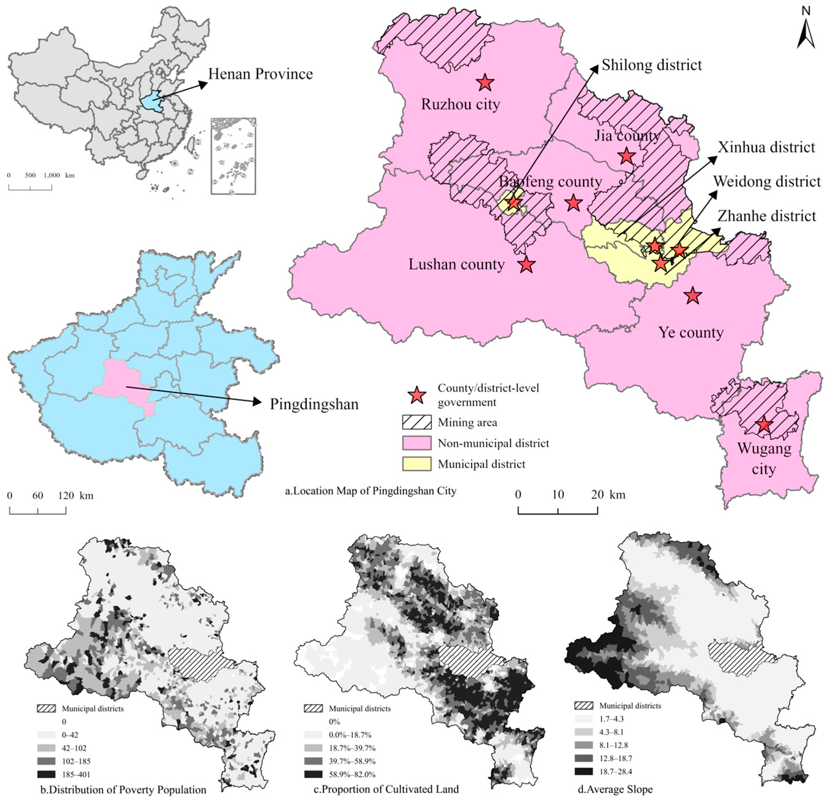
Figure 1. Study Area and Village-Level Spatial Characteristics of Pingdingshan City.
Sustainability 17 09704 g001
Figure 2. Rural Household Poverty Alleviation and Development Path Identification Framework.
Sustainability 17 09704 g002
Figure 3. Feature Importance and SHAP Value Distributions of Key Indicators. Color represents the feature value from low (blue) to high (red). Grey rectangles indicate the mean absolute SHAP values (feature importance), and the grey vertical line denotes the baseline (SHAP = 0).
Sustainability 17 09704 g003
Figure 4. Heatmap of Cluster Centers in the Initial State.
Sustainability 17 09704 g004
Figure 5. Spatial Distribution of Clustering Results in the Initial State.
Sustainability 17 09704 g005
Figure 8. Heatmap of Cluster Centers in the Return-to-Poverty Process.
Sustainability 17 09704 g008
Figure 9. Spatial Distribution of Clustering Results in the Return-to-Poverty Process.
Sustainability 17 09704 g009
Figure 10. Unstable Poverty Alleviation Process: Heatmap of Cluster Centers.
Sustainability 17 09704 g010
Figure 11. Unstable Poverty Alleviation Process: Spatial Distribution of Clustering Results.
Sustainability 17 09704 g011
Figure 12. Overall Distribution of Household Poverty Alleviation and Development Pathways.
Sustainability 17 09704 g012
Figure 13. Variation within the S I P S Pathway.
Sustainability 17 09704 g013
Figure 14. Variation within the S I P U and S I P U P S Pathways.
Sustainability 17 09704 g014
Figure 15. Variation within the S I P S P R P S Pathway.
Sustainability 17 09704 g015
Figure 16. Spatial Distribution of Poverty Alleviation Pathways for S I 1 and S I 3 across Different Processes.
Sustainability 17 09704 g016
Figure 17. Spatial Distribution of Poverty Alleviation Pathways for S I 4 and S I 5 across Different Processes.
Sustainability 17 09704 g017
Figure 18. Mechanisms of Pathways to Stable Poverty Alleviation.
Sustainability 17 09704 g018
Table 1. Symbols, states, and processes in household poverty alleviation and development pathways.
SymbolTypeEnglish TermDefinition
S P StatePoverty StateHousehold has not yet escaped poverty
S S StateStable Poverty Alleviation StateHousehold has escaped poverty and is unlikely to fall back
S U StateUnstable Poverty Alleviation StateHousehold has escaped poverty but remains at risk of returning
S I StateInitial StateHousehold’s status when first included in monitoring and support system
P S ProcessStable Poverty Alleviation ProcessTransition from S P or S U to S S , with sustained stability
P R ProcessReturn to Poverty ProcessTransition from S S back to S P or S U due to internal or external shocks
P U ProcessUnstable Poverty Alleviation ProcessFluctuation between S P and S U without reaching S S
Disclaimer/Publisher’s Note: The statements, opinions and data contained in all publications are solely those of the individual author(s) and contributor(s) and not of MDPI and/or the editor(s). MDPI and/or the editor(s) disclaim responsibility for any injury to people or property resulting from any ideas, methods, instructions or products referred to in the content.