Abstract
Air density and pressure above the Earth’s surface in the tropospheric region depend on altitude relative to sea level. When a given amount of pollutant gas enters the atmosphere at sea level, it produces a contaminated air mixture; if the same amount of pollutant gas enters the atmosphere at a location situated at higher altitude, atmospheric pollution certainly also occurs. However, the relative compositions are not the same in both cases due to the greater air density present at sea level compared to the air density at higher altitude. Current regulatory frameworks, including the National Ambient Air Quality Standards (NAAQS) of the United States Environmental Protection Agency and the Air Quality Guidelines (AQG) of the World Health Organization, establish constant numerical values for air quality standards uniformly applicable at all geographic locations, regardless of altitude, resulting in inadequate health protection for millions of people. To address this critical gap, a universal adjustment factor for atmospheric pollutant gas concentrations at different altitudes has been derived from first principles of atmospheric physics; this factor is , where h is expressed in meters, assuming air at constant temperature given that small temperature variations do not substantially influence atmospheric density and pressure or pollutant concentrations at different altitudes. The factor was systematically applied to the NAAQS and WHO AQG, demonstrating that for altitudes of 3500 m, representative of cities such as Cusco, Peru, the adjusted standards are approximately 67% of the nominal values established at sea level, preserving the gaseous pollutant–air proportionality. Experimental measurements of atmospheric density in six Peruvian cities distributed along an altitudinal gradient of 0–3826 m validated the theoretical model with relative deviations less than 5%, confirming the physical consistency of the derived factor. The importance of this research lies in adequately regulating air quality standards related to public health and the environment, supporting the implementation of equitable environmental policies aligned with the United Nations (UN) 2030 Sustainable Development Goals, and establishing that the constant values defined at sea level must be adjusted according to the aforementioned factor when geographic altitude is considered.
1. Introduction
Regulations on atmospheric air quality constitute the primary framework for protecting public health against airborne pollutants globally [1,2,3]. The National Ambient Air Quality Standards (NAAQS) established by the United States Environmental Protection Agency (EPA) and the Air Quality Guidelines (AQG) developed by the World Health Organization (WHO) define concentration thresholds for criteria pollutants that, when exceeded, represent significant health risks. The WHO estimates that 99% of the world’s population breathes air that exceeds guideline values, contributing to more than 6 million premature deaths annually [1,4,5]. Epidemiological evidence demonstrates that exposure to air pollution increases human morbidity and mortality, with spatial and temporal trends in the disease burden attributable to air pollution showing significant variations between regions and periods from 1990 to 2015 [6]. However, the current implementation of these regulatory frameworks assumes uniform applicability in all geographic locations, regardless of altitude. This assumption is problematic because approximately 500 million people, representing 6.58% of the world’s population, reside above 1500 m above sea level (m.a.s.l.), where atmospheric pressure and density differ substantially from sea-level conditions [7]. High-altitude cities such as La Paz, Bolivia (3640 m.a.s.l.), Quito, Ecuador (2800 m.a.s.l.), and Cusco, Peru (3400 m.a.s.l.), apply identical numerical standards to those of coastal cities despite fundamental differences in the atmospheric physics governing the behavior of atmospheric pollutants and human exposure to such pollutants [8,9,10]. This regulatory omission may misrepresent the actual health risks to high-altitude populations and compromise public health protection in these regions. Addressing this gap is essential for achieving equitable environmental governance aligned with the UN 2030 Sustainable Development Goals, particularly SDG 3 (Good Health and Well-being), SDG 10 (Reduced Inequalities), and SDG 11 (Sustainable Cities and Communities) [11,12].
The physical basis for altitude-dependent variation in pollutant concentrations derives from the exponential decrease in atmospheric pressure with elevation, described by the barometric equation, where atmospheric pressure at 3000 m.a.s.l. approximates 70% of sea-level values [13,14,15]. This pressure reduction directly affects air density, which determines the mass of atmospheric constituents per unit volume. Çengel and Cimbala [16] demonstrate that air density decreases exponentially with altitude following a similar exponential dependence. When regulatory agencies establish concentration-based standards (μg/m3, ppm, or ppb), they implicitly reference sea-level atmospheric conditions as defined by international standards organizations: the International Union of Pure and Applied Chemistry (IUPAC), the National Institute of Standards and Technology (NIST), and the Environmental Protection Agency (EPA) specify standard temperature and pressure conditions [17,18,19]. A given mass of pollutant dispersed in one cubic meter at high altitude occupies the same volume but within less dense air compared to the same mass of pollutant and same unit volume at sea level, producing different relative compositions in the air–pollutant mixture. Health implications depend on the relationship between pollutant mass and air mass, the actual exposure metric, rather than solely on volumetric concentrations [20]. This fundamental physical discrepancy between concentration measurement conventions and physical principles of gaseous pollutant–air proportionality creates a systematic bias in altitude regulatory applications.
Despite its early recognition, research addressing the effects of altitude on air quality standards remains limited. The U.S. EPA [21] identified altitude as a factor influencing air pollution due to atmospheric pressure variation but provided no quantitative adjustment framework. Bravo and Urone [22] recommended using dose relationships or respiratory rates to adjust U.S. air quality standards to ensure adequate health protection in high-altitude cities, noting that numerically appropriate AQS values at altitude should be lower than sea-level standards. More recently, Bravo Alvarez et al. [23] demonstrated that air quality standards for particulate matter (PM) require altitude-specific adjustment, proposing empirical correction factors for nine high-altitude Latin American cities. Their methodology, based on ideal gas law principles and concentration definitions, established that PM standards must account for each city’s specific elevation. However, their approach was limited to particulate matter and discrete urban centers, lacking a universal theoretical framework applicable to all altitudes and pollutant types. A recent scoping review by Rueda-Torres et al. [8] comprehensively examined altitude adjustment criteria for air quality standards, analyzing the existing literature on proposed adjustments, regulatory frameworks in high-altitude countries, and altitude-influenced pollutants. This review identified critical research gaps and the absence of systematic regulatory incorporation of altitude corrections despite documented physical necessity.
Analogous altitude considerations appear in related fields, but environmental regulations have not systematically incorporated such corrections. Aeronautical medicine adjusts oxygen requirements with elevation [24], exercise physiology modifies prescription parameters for altitude training [25], and meteorology routinely corrects pressure measurements to their sea-level equivalents for standardized reporting [26]. Engineering applications recognize altitude-dependent effects on atmospheric density: Yu et al. [27] demonstrated that diesel and biodiesel consumption in engines increases with altitude due to reduced intake air mass flow at elevation, while Perez and Boehman [28] showed that turbochargers in single-cylinder diesel engines for unmanned aerial vehicles compensate for lower air density at high altitudes through electromechanical systems. Despite these precedents across multiple disciplines, current regulatory frameworks including the EPA NAAQS [29] and WHO guidelines [1] specify fixed concentration limits without altitude considerations, potentially leaving high-altitude populations insufficiently protected or imposing inefficient restrictions on industrial and transportation activities.
This regulatory gap affects millions of inhabitants of mountainous regions in the Andes, Himalayas, Alps, and Rocky Mountains. In Latin America alone, millions live at elevations above 2500 m.a.s.l. [30,31], where atmospheric density approximates 75% of sea-level values. Application of unadjusted standards at such altitudes leads to systematic underestimation of actual pollutant exposure, i.e., the physicochemical proportionality of the gaseous pollutant–air mixture is not being taken into account. Currently, no universal altitude adjustment factor based on fundamental principles of atmospheric physics exists to translate sea-level air quality standards to altitude-appropriate values.
This study addresses this critical gap by deriving a universal altitude adjustment factor for gaseous pollutant air quality standards from first principles of atmospheric physics. Our specific contributions include the following: (1) a rigorous mathematical derivation of the adjustment factor from hydrostatic equilibrium and ideal gas law principles, incorporating standard conditions established by IUPAC, EPA, and NIST; (2) demonstration of the factor’s applicability to gaseous criteria pollutants across different regulatory frameworks (EPA NAAQS, WHO guidelines); and (3) quantification of adjustment magnitudes for representative high-altitude population centers.
Implementation of altitude-adjusted air quality standards could significantly impact environmental policy and public health protection for the ∼500 million inhabitants residing above 1500 m globally. By providing a universally applicable correction factor, this work enables regulatory agencies to establish elevation-appropriate concentration limits that maintain equivalent health protection across the entire range of human habitation altitudes, from sea level to cities even exceeding 5000 m.a.s.l.
2. Methodology
2.1. Analysis of Atmospheric Pressure Variation with Altitude
Rigorous quantification of atmospheric pressure and density variation with altitude constitutes the physical foundation for understanding how effective concentrations of gaseous pollutants are modified with geographic elevation. The analytical development begins from the hydrostatic equilibrium of a differential atmospheric fluid element (Figure 1), whose vertical force balance establishes that the pressure gradient must equilibrate the weight of the air column:
where p represents atmospheric pressure (Pa), h the altitude above sea level (m), the air density (kg/m3), and g the gravitational acceleration (9.80 m/s2). This fundamental differential equation requires a constitutive relationship for its resolution. The ideal gas equation of state provides the necessary thermodynamic closure:
where p represents the atmospheric pressure (Pa), V the volume (m3), n the number of moles of gas, R the universal gas constant (8.314 J/mol·K), and T the absolute temperature (K).
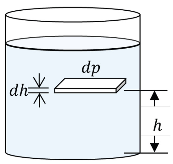
Figure 1.
Differential atmospheric fluid element in hydrostatic equilibrium showing vertical pressure gradient.
The molar mass of air M (kg/mol) relates total mass to the number of moles:
where m denotes the total mass of air (kg) and n the number of moles (mol).
Density is defined as
where represents the air density (kg/m3), m the mass (kg), and V the volume (m3). The combination of Equations (2)–(4) establishes the fundamental relationship between density, pressure, and temperature that characterizes the thermodynamic behavior of atmospheric air:
Substituting Equation (5) into Equation (1) yields
Integration of Equation (6) requires specifying the temperature profile with altitude. For analysis of regulatory standards in the troposphere, where temperature variations (−6.5 °C/km according to [26]) are moderate compared to absolute temperature (∼300 K), the isothermal approximation is adopted. This simplification, used in first-order barometry [32], leads to the exponential solution
where represents atmospheric pressure at sea level, whose adopted standard value is
This barometric solution describes the exponential decay of pressure with altitude, a result validated empirically [13,14,15].
Numerical evaluation of the barometric exponent depends on standard temperature and pressure conditions adopted by different organizations. Table 1 summarizes definitions and resulting coefficients.

Table 1.
Standard temperature and pressure conditions and barometric coefficients.
For IUPAC ():
For NIST ():
For EPA ():
Figure 2 shows these curves. To quantify differences, Table 2 presents relative errors between standards at various altitudes.
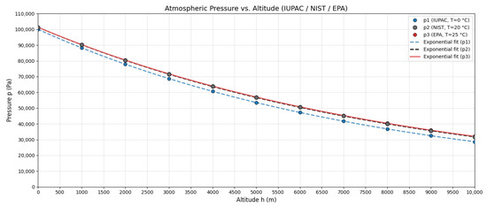
Figure 2.
Atmospheric pressure as a function of altitude for IUPAC (T = 273.15 K), NIST (T = 293.15 K), and EPA (T = 298.15 K) standards according to Equations (12)–(14).
Table 2.
Relative errors (%) between pressures calculated with different standards.
EPA vs. NIST differences remain < 1% up to 5000 m, validating the use of EPA standards for subsequent development, consistent with regulatory practices.
2.2. Atmospheric Density as a Function of Altitude
Atmospheric density follows a law analogous to that of pressure [14]. From Equations (5) and (7),
Adopting EPA standards (T = 298.15 K):
According to Çengel and Cimbala [16], the reference value for air at 1 atm and 20 °C is
Therefore,
Figure 3 illustrates this variation.
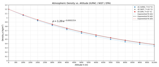
Figure 3.
Atmospheric density as a function of altitude according to the exponential model (Equation (18)).
Since
then if we assume that V = 1 m3, the mass at sea level is m0 = 1.20 kg, which means that the air mass as a function of altitude is given by
2.3. Composition of Tropospheric Air and Population Distribution by Altitude
Tropospheric air composition is remarkably constant up to ∼10–11 km (troposphere boundary) [32,33]. This validates treating air as a homogeneous ideal mixture in the air quality context. Table 3 presents mass percentages of the main components (standard conditions, 1 m3 at 20 °C, 1 atm) [13,34], and Table 4 shows volume percentages [34].
Table 3.
Mass percentages of the main components of dry air under standard conditions (1 m3 at 20 °C, 1 atm).
Table 4.
Volume percentages of the main components of dry air under standard conditions.
Figure 4 shows the constancy of these proportions in the troposphere.
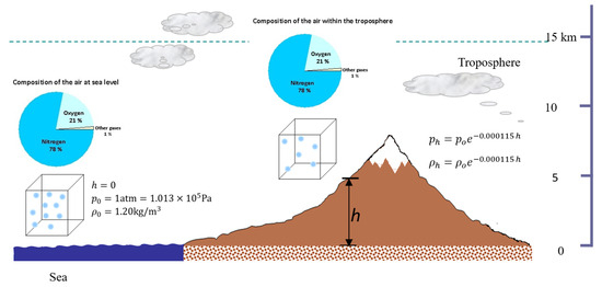
Figure 4.
Volume percentage composition of air (N2 78%, O2 21%, others 1%) constant at different tropospheric altitudes.
The practical relevance of the above is evidenced by population distribution by altitude: ∼93.42% of the world’s population inhabits between 0 and 1500 m, while ∼500 million (6.58%) reside above 1500 m [7]. Figure 5 highlights that at >1500 m, atmospheric density and pressure are <82% of sea-level values, with direct implications for effective pollutant exposure.
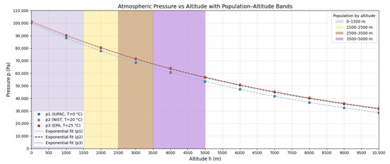
Figure 5.
World population distribution by altitude ranges: 93.42% resides between 0–1500 m and 6.58% above 1500 m.
2.4. Derivation of the Adjustment Factor Using the Proportions Method
The adjustment approach recognizes that equivalent health protection in chronic exposure requires maintaining constant mass fraction of the pollutant in the inhaled air–pollutant mixture. This principle is founded on the fact that cumulative inhaled dose (determinant in chronic effects) is proportional to the product of the pollutant mass fraction in the breathed mixture and total ventilatory volume. Unlike acute effects (where partial pressure governs immediate alveolar diffusion), prolonged exposure, the basis of regulatory hourly/daily/annual averages, is determined by total inhaled mass. This analysis requires conservation of mass proportions between altitudes.
Figure 6 illustrates the 1 m3 control volume at sea level and at altitude h, with partition between clean air mass and pollutant mass. The total masses are
where the subscripts a and s denote clean air and pollutant substance; 0 and h indicate sea level and altitude h.
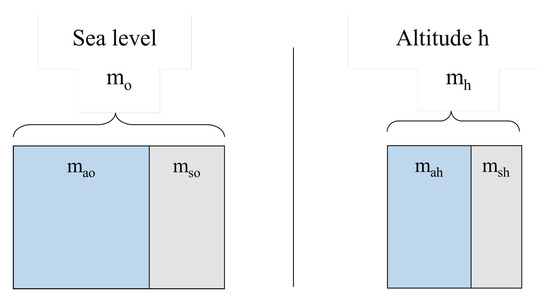
Figure 6.
Unit control volume (1 m3) showing air–pollutant mass partition at sea level (, ) and at altitude h (, ).
Air is a homogeneous gas mixture [13]. If, additionally, a gaseous pollutant enters a control volume, the gaseous pollutant–air mixture maintains a uniform composition; therefore, any extracted portion is representative of the whole. This physicochemical foundation enables mathematical proportionality between the sea-level case and the case at altitude h. Specifically, if at sea level the ratio between pollutant mass and total mixture mass is , and at altitude h the corresponding ratio is ; the homogeneity of the mixture implies that these ratios are equal:
Rearranging,
Substituting Equations (21) and (22),
and expanding them,
from which
Solving for ,
Using Equation (20) for air masses,
and therefore,
Dividing by m3,
Defining the mass concentration ,
Thus, the universal conversion (adjustment) factor is
with h in meters. This central result establishes that, to preserve equivalent health protection between altitudes, mass concentration limits must decrease exponentially with elevation.
3. Results and Discussion
3.1. Application of the Adjustment Factor to International Regulatory Frameworks
Application of the obtained adjustment factor to air quality standards was performed by direct multiplication (Equation (33)). Table 5 and Table 6 show systematic application of the factor to the National Ambient Air Quality Standards (NAAQS) of the EPA and to the Air Quality Guidelines of the WHO for representative altitudes.
Table 5.
EPA standards (NAAQS) at sea level and adjusted by altitude (criteria gases).
Table 6.
WHO guidelines (2021) at sea level and adjusted by altitude (gases).
For altitudes of 3500 m (e.g., Cusco ∼3400 m and La Paz ∼3640 m), adjusted standards are ∼67% of nominal values. This does not imply lower protection but rather proportionality in the (gaseous pollutant–air) mixture; maintaining 100 ppb of NO2 without adjustment at 3500 m elevates the NO2/air mass fraction by around 50% relative to sea level, and adjustment to 66.86 ppb preserves the original fraction.
Figure 7 illustrates the fundamental principle of altitude adjustment: for any gaseous pollutant entering the air, concentration decreases exponentially with geographic elevation according to Equation (32). This general relationship is independent of the pollutant type, regulatory framework (EPA, WHO, national regulations), and unit system employed (volumetric such as ppm/ppb or mass-based such as μg/m3/mg/m3), since the factor f is dimensionless and derives exclusively from the variation in atmospheric density with altitude.
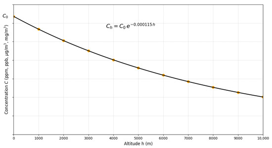
Figure 7.
Universal variation in gaseous pollutant concentration with altitude according to . The vertical axis represents concentration in arbitrary units (ppm, ppb, μg/m3, mg/m3), applicable to any gaseous criteria pollutant. Markers illustrate altitudes of representative high-altitude cities.
Quantitative implications are significant across the pollutant spectrum. For O3 (peak season, WHO guideline of 60 μg/m3), at 3500 m the adjusted value is 40.12 μg/m3 (33.1% reduction), consistent with . For annual NO2 (WHO guideline of 10 μg/m3), the adjusted standard decreases to 6.69 μg/m3 (3500 m) and 5.96 μg/m3 (4500 m). Markers in the figure correspond to altitudes of representative urban centers, Quito (2850 m), Cusco (3400 m), and La Paz (3640 m), evidencing that, for these cities, adjusted standards vary between 67 and 75% of nominal sea-level values. At 1500 m, (reduction ∼16%); above 2500 m, corrections exceed 25%, magnitudes that are critical given that air quality standards are based on narrow margins of public health protection [6], where ignoring these corrections would lead to consequent risks.
The universality of the adjustment factor allows its direct application through simple multiplication of the nominal standard by for the local altitude, without need for pollutant-specific empirical recalibration. This property contrasts with previous approaches requiring discrete city-by-city adjustments [23] and underscores the advantage of a derivation based on first physical principles over ad hoc methodologies. Nevertheless, the model’s scope is delimited to gaseous criteria pollutants (CO, NO2, O3, SO2) that exhibit ideal gas behavior under tropospheric conditions.
The isothermal approximation (Equation (7)) introduces quantifiable uncertainties. With the actual thermal gradient of −6.5 °C/km [26], up to 5000 m, deviation in remains below 10%; propagated to the factor f, this uncertainty translates to ±2% (2500 m) and ±5% (5000 m), magnitudes comparable to seasonal meteorological variability and substantially smaller than the 35% effect induced by altitude.
3.2. Application to High-Altitude Urban Centers in Peru and Experimental Validation
The Peruvian altitudinal gradient (0–3826 m) allows a representative test. Table 7 summarizes in situ measurements (altitude, h; temperature, ; pressure, ; humidity, ) and density inferred via .
Table 7.
Atmospheric magnitudes measured in cities of southern Peru.
Density decreases from 1.18 to 0.77 kg/m3 (35% reduction), consistent with theory (Equation (18)). As shown in Figure 8, the fit between the experimental data (points) and theoretical model (line) presents deviations < 5%; the discrepancy in Mollendo is attributed to humidity (humid air is less dense).
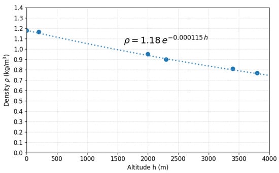
Figure 8.
Experimental atmospheric density (points) versus theoretical model (line) for six Peruvian cities along a 0–3826 m gradient.
Figure 9 visualizes the variation in air mass contained in 1 m3 as a function of altitude, showing exponential decay from kg (Mollendo) to kg (Puno). This 35% reduction in air mass available to dilute pollutants has direct implications: if a source emits equal mass, , in Mollendo and Puno, mass concentration in Puno will be ∼1.53 times higher solely due to less diluting air. For Puno ( m), , so limits must be 65.3% of nominal values for equivalence.
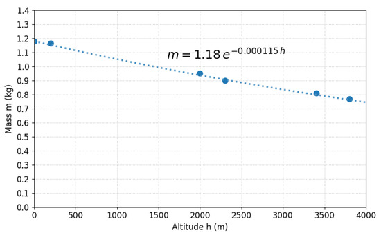
Figure 9.
Air mass in unit volume (1 m3) versus altitude for Peruvian cities. Exponential decay from 1.18 kg (Mollendo) to 0.77 kg (Puno).
Figure 10 presents a schematic diagram with the relative location of the six cities on the Andean altitudinal profile, with 1 m3 cubes representing the control volume at each location. Although volume remains constant (geometric invariance), air masses vary exponentially, as quantified in Table 7.
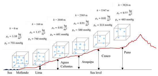
Figure 10.
Location of Peruvian cities on Andean altitudinal profile with constant control volume (1 m3) and variable air masses.
Coherence between data (Table 7) and isothermal model validates the approximation: recalculating with measured T (non-isothermal model), differences versus constant T of 298.15 K are <4% (average 2.1%). Humidity (41–80%) reduces by 2–3% depending on conditions, a minor effect compared to the 35% due to altitude.
In regulatory terms, applying nominal standards to Cusco (3347 m, ) would imply mass fractions ∼1.49 times higher than those at sea level for the same numerical limit, compromising the intended protection.
Model scope: is for the criterion gases (CO, NO2, O3, SO2) under tropospheric conditions. Extension to PM requires other physicochemical processes [23]; in general, the factor for gases is a lower bound for particles. Future work should address aerosol dynamics coupled to density variation, together with measurements along altitudinal gradients (Table 8).
Table 8.
Altitude-adjusted standards for Peruvian cities ().
4. Conclusions
Based on rigorous physical foundations grounded in hydrostatic equilibrium and ideal gas thermodynamics, a universal altitude adjustment factor for air quality standards of gaseous pollutants has been derived:
where h is altitude in meters. This factor compensates for the exponential decay of atmospheric density with geographic elevation and preserves gaseous pollutant–air proportionality at different altitudes. Systematic application to the National Ambient Air Quality Standards (NAAQS) of the EPA and the Air Quality Guidelines (AQG) of the WHO showed that, for altitudes of 3500 m (e.g., Cusco, La Paz), adjusted standards should be approximately 67% of nominal values defined at sea level, in order to sustain an equivalent level of health protection. Experimental validation through atmospheric density measurements in six Peruvian cities along 0–3826 m confirmed the consistency of the theoretical model, with relative deviations below 5%, which supports the isothermal approximation employed.
A critical finding is that direct application of unadjusted standards in high-altitude cities results in inadequate protection: maintaining a limit of 100 ppb of NO2 at ∼3400 m implies cumulative exposure approximately 49% higher relative to that intended at sea level, compromising public health objectives. Unlike previous empirical approaches limited to specific pollutants or cities, the proposed factor is founded on invariant physical properties of the atmosphere, allowing its universal application to gaseous pollutants (CO, NO2, O3, SO2) independent of the regulatory framework or unit system.
Incorporation of this factor into national and international environmental legislation will enable equivalent health protection for the ∼500 million inhabitants residing above 1500 m globally, contributing to sustainable and equitable environmental governance. This work directly supports the UN 2030 Agenda for Sustainable Development by providing science-based tools for environmental policy-making that address health inequities across diverse geographic contexts, particularly advancing SDG 3 (Good Health and Well-being), SDG 10 (Reduced Inequalities), and SDG 11 (Sustainable Cities and Communities). By enabling altitude-appropriate air quality regulations, this research promotes environmental justice and long-term public health sustainability in high-altitude regions worldwide. Future work should extend the model to particulate matter and integrate these findings into comprehensive sustainability frameworks for mountainous communities.
Author Contributions
Conceptualization, J.W., A.O., R.C., and B.W.; methodology, J.W., A.O., R.C., B.W., and A.Z.; validation, J.W., A.O., R.C., and A.Z.; formal analysis, J.W., R.C., B.W., and A.Z.; investigation, J.W., A.O., R.C., B.W., and A.Z.; writing—original draft preparation, J.W., R.C., and B.W.; writing—review and editing, J.W., A.O., B.W., and A.Z.; visualization, J.W.; supervision, J.W., A.O., R.C., B.W., and A.Z. All authors have read and agreed to the published version of the manuscript.
Funding
This research received no external funding.
Institutional Review Board Statement
Not applicable.
Informed Consent Statement
Not applicable.
Data Availability Statement
The data presented in this study are available on request from the corresponding author.
Acknowledgments
We are grateful to Universidad Nacional de San Antonio Abad del Cusco and to the Centro de Investigación de Energía y Atmósfera for providing the facilities and resources necessary to develop the theoretical and practical aspects of this research.
Conflicts of Interest
The authors declare no conflicts of interest.
References
- World Health Organization. WHO Global Air Quality Guidelines: Particulate Matter (PM2.5 and PM10), Ozone, Nitrogen Dioxide, Sulfur Dioxide and Carbon Monoxide; Technical report; World Health Organization: Geneva, Switzerland, 2021. [Google Scholar]
- Siddique, A.; Al-Shamlan, M.Y.M.; Al-Romaihi, H.E.; Khwaja, H.A. Beyond the outdoors: Indoor air quality guidelines and standards— Challenges, inequalities, and the path forward. Rev. Environ. Health 2025, 40, 21–35. [Google Scholar] [CrossRef] [PubMed]
- Tewari, S.; Pandey, N.; Dong, J. Air Quality Legislation in Australia and Canada—A Review. Challenges 2024, 15, 43. [Google Scholar] [CrossRef]
- Raza, W.A.; Mahmud, I.; Rabie, T.S. Breathing Heavy: New Evidence on Air Pollution and Health in Bangladesh; International Development in Focus, World Bank: Washington, DC, USA, 2023. [Google Scholar] [CrossRef]
- Khomenko, S.; Cirach, M.; Pereira-Barboza, E.; Mueller, N.; Barrera-Gómez, J.; Rojas-Rueda, D.; de Hoogh, K.; Hoek, G.; Nieuwenhuijsen, M. Premature mortality due to air pollution in European cities: A health impact assessment. Lancet Planet. Health 2021, 5, e121–e134. [Google Scholar] [CrossRef] [PubMed]
- Cohen, A.J.; Brauer, M.; Burnett, R.; Anderson, H.R.; Frostad, J.; Estep, K.; Balakrishnan, K.; Brunekreef, B.; Dandona, L.; Dandona, R.; et al. Estimates and 25-year trends of the global burden of disease attributable to ambient air pollution: An analysis of data from the Global Burden of Diseases Study 2015. Lancet 2017, 389, 1907–1918. [Google Scholar] [CrossRef] [PubMed]
- Tremblay, J.C.; Ainslie, P.N. Global and country-level estimates of human population at high altitude. Proc. Natl. Acad. Sci. USA 2021, 118, e2102463118. [Google Scholar] [CrossRef] [PubMed]
- Rueda-Torres, L.V.; Warthon-Ascarza, J.; Pacsi-Valdivia, S. Adjustment Criteria for Air-Quality Standards by Altitude: A Scoping Review with Regulatory Overview. Int. J. Environ. Res. Public Health 2025, 22, 1053. [Google Scholar] [CrossRef] [PubMed]
- Parra, R. Modeling PM2.5 Levels Due to Combustion Activities and Fireworks in Quito (Ecuador) for Forecasting Using WRF-Chem. Atmosphere 2025, 16, 495. [Google Scholar] [CrossRef]
- Warthon, J.; Zamalloa, A.; Olarte, A.; Warthon, B.; Miranda, I.; Zamalloa-Puma, M.M.; Ccollatupa, V.; Ormachea, J.; Quispe, Y.; Jalixto, V.; et al. A Comprehensive Assessment of PM2.5 and PM10 Pollution in Cusco, Peru: Spatiotemporal Analysis and Development of the First Predictive Model (2017–2020). Sustainability 2025, 17, 394. [Google Scholar] [CrossRef]
- United Nations, Department of Economic and Social Affairs, Division for Sustainable Development Goals (DSDG). The 17 Goals|Sustainable Development, 2015. Official United Nations Page for the Sustainable Development Goals. Available online: https://sdgs.un.org/goals (accessed on 17 October 2025).
- United Nations. Transforming Our World: The 2030 Agenda for Sustainable Development. United Nations Sustainable Development Goals (website), 2015. Adopted by the UN General Assembly in September 2015. Available online: https://sdgs.un.org/2030agenda (accessed on 17 October 2025).
- Andrews, D.G. An Introduction to Atmospheric Physics, 2nd ed.; Cambridge University Press: Cambridge, UK, 2010; p. 248. [Google Scholar] [CrossRef]
- Sears, F.W.; Zemansky, M.W.; Young, H.D.; Freedman, R.A. University Physics with Modern Physics, 11th ed.; Pearson Addison Wesley: San Francisco, CA, USA, 2004; p. 1374. [Google Scholar]
- Tipler, P.A.; Mosca, G. Physics for Scientists and Engineers, 6th ed.; W. H. Freeman: New York, NY, USA, 2007; p. 1172. [Google Scholar]
- Çengel, Y.A.; Cimbala, J.M. Fluid Mechanics: Fundamentals and Applications, 1st ed.; McGraw-Hill Series in Mechanical Engineering; McGraw-Hill: New York, NY, USA, 2006; p. 992. [Google Scholar]
- Levine, I.N. Physical Chemistry, 6th ed.; McGraw-Hill Education: New York, NY, USA, 2009; p. 1008. [Google Scholar]
- Doiron, T.D. 20 °C—A Short History of the Standard Reference Temperature for Industrial Dimensional Measurements. J. Res. Natl. Inst. Stand. Technol. 2007, 112, 1–23. [Google Scholar] [CrossRef] [PubMed]
- U.S. Environmental Protection Agency. National Primary and Secondary Ambient Air Quality Standards. 40 CFR Part 50, 1998. Federal Register, Volume 63, No. 25, pp. 7274–7275, 6 February 1998. Available online: https://www.govinfo.gov/content/pkg/FR-1998-02-06/pdf/98-2957.pdf (accessed on 9 September 2025).
- Baird, C.; Cann, M. Química Ambiental, 2nd ed.; Editorial Reverté: Barcelona, Spain, 2014. [Google Scholar]
- U.S. Environmental Protection Agency. Altitude as a Factor in Air Pollution; Technical Report EPA/600/9-78/015; U.S. Environmental Protection Agency: Washington, DC, USA, 1978. [Google Scholar]
- Bravo, A.; Urone, P. The Altitude: A Fundamental Parameter in the Use of Air Quality Standards. J. Air Pollut. Control Assoc. 1981, 31, 264–265. [Google Scholar] [CrossRef]
- Bravo Alvarez, H.; Sosa Echeverria, R.; Sanchez Alvarez, P.; Krupa, S. Air Quality Standards for Particulate Matter (PM) at high altitude cities. Environ. Pollut. 2013, 173, 255–256. [Google Scholar] [CrossRef] [PubMed]
- Shaw, D.M.; Cabre, G.; Gant, N. Hypoxic Hypoxia and Brain Function in Military Aviation: Basic Physiology and Applied Perspectives. Front. Physiol. 2021, 12, 665821. [Google Scholar] [CrossRef] [PubMed]
- Doutreleau, S.; Ulliel-Roche, M.; Hancco, I.; Bailly, S.; Oberholzer, L.; Robach, P.; Brugniaux, J.V.; Pichon, A.; Stauffer, E.; Perger, E.; et al. Cardiac remodelling in the highest city in the world: Effects of altitude and chronic mountain sickness. Eur. J. Prev. Cardiol. 2022, 29, 2154–2162. [Google Scholar] [CrossRef] [PubMed]
- NOAA; NASA; USAF. U.S. Standard Atmosphere, 1976; Technical Memorandum NOAA-S/T-76-1562, NASA-TM-X-74335, National Oceanic and Atmospheric Administration, National Aeronautics and Space Administration, United States Air Force: 1976. Available online: https://ntrs.nasa.gov/citations/19770009539 (accessed on 8 September 2025).
- Yu, L.; Ge, Y.; Tan, J.; He, C.; Wang, X.; Liu, H.; Zhao, W.; Guo, J.; Fu, G.; Feng, X.; et al. Experimental investigation of the impact of biodiesel on the combustion and emission characteristics of a heavy duty diesel engine at various altitudes. Fuel 2014, 115, 220–226. [Google Scholar] [CrossRef]
- Perez, P.L.; Boehman, A.L. Performance of a single-cylinder diesel engine using oxygen-enriched intake air at simulated high-altitude conditions. Aerosp. Sci. Technol. 2010, 14, 83–94. [Google Scholar] [CrossRef]
- U.S. Environmental Protection Agency. NAAQS Table. Criteria Air Pollutants, 2022. National Ambient Air Quality Standards for Six Criteria Pollutants. Available online: https://www.epa.gov/criteria-air-pollutants/naaqs-table (accessed on 8 September 2025).
- Richalet, J.P.; Hermand, E.; Lhuissier, F.J. Cardiovascular physiology and pathophysiology at high altitude. Nat. Rev. Cardiol. 2024, 21, 75–88. [Google Scholar] [CrossRef] [PubMed]
- Sharma, P.; Mohanty, S.; Ahmad, Y. A study of survival strategies for improving acclimatization of lowlanders at high-altitude. Heliyon 2023, 9, e14929. [Google Scholar] [CrossRef] [PubMed]
- Manahan, S.E. Environmental Chemistry, 7th ed.; Lewis Publishers: Boca Raton, FL, USA, 2000; p. 912. [Google Scholar]
- Chang, R.; Goldsby, K.A. Química, 11th ed.; McGraw-Hill Interamericana: Mexico City, Mexico, 2013; p. 1107. [Google Scholar]
- Saha, K. The Earth’s Atmosphere: Its Physics and Dynamics, 1st ed.; Springer: Berlin/Heidelberg, Germany, 2008; p. 367. [Google Scholar] [CrossRef]


Disclaimer/Publisher’s Note: The statements, opinions and data contained in all publications are solely those of the individual author(s) and contributor(s) and not of MDPI and/or the editor(s). MDPI and/or the editor(s) disclaim responsibility for any injury to people or property resulting from any ideas, methods, instructions or products referred to in the content. |
© 2025 by the authors. Licensee MDPI, Basel, Switzerland. This article is an open access article distributed under the terms and conditions of the Creative Commons Attribution (CC BY) license (https://creativecommons.org/licenses/by/4.0/).