Abstract
Urban rail transit, as a green, environmentally friendly, safe, and efficient mode of transportation, plays a crucial role in urban sustainable development. However, the influencing mechanism of build environment factors on rail transit ridership still needs to be further investigated. Also, the interaction effects between these factors have not been considered. This study aims to explore the relationship and impact of built environmental factors on metro ridership. The research employs the Multiscale Geographically Weighted Regression (MGWR) model to analyze the temporal and spatial effects of built environmental factors on the rail transit ridership. The GeoDetector model is utilized to investigate the interactive effects of these factors on rail transit ridership. The Shanghai Metro ridership data and built environment data are applied to validate the model. Based on data analysis results, we found that Food & Beverages and Accommodation services, respectively, have the greatest impact on metro ridership on weekdays and weekends. Furthermore, the interaction effects between other variable and Land use diversity significantly enhance rail transit ridership, validating the promoting effect of land use diversity on metro ridership. By proposing recommendations for relevant urban planning and policy formulation, we can foster the sustainable development of urban rail transit.
1. Introduction
In recent years, rapid urbanization has triggered a surge in private vehicle adoption, exacerbating traffic congestion, elevated carbon emissions, and environmental degradation globally [1]. As a sustainable mobility solution, urban rail transit systems—characterized by speed, efficiency, and low carbon footprint—have proven effective in mitigating traffic congestion [2]. Consequently, many countries have embraced the public transit priority policy, spurring a surge in urban rail transit construction that is expanding from Western countries to emerging markets [3,4].
To optimize rail transit system planning, identifying determinants of ridership has become a focal research agenda in transportation and urban planning disciplines. Examining the correlation between rail transit ridership and built environment (BE) factors holds paramount importance across urban planning, rail transit design, and passenger flow management realms [5,6]. Consequently, numerous investigations have probed the links between urban rail transit ridership and BE factors employing diverse models. Regression-based Direct Ridership Models (DRMs) have been extensively utilized to scrutinize the influence of BE factors on rail transit ridership in metropolitan centers such as Seoul [7], Madrid [8], San Diego [9], Beijing [10] and Shanghai [11]. While DRMs are intuitive and offer strong explanatory ability, they assume that the observed values, such as passenger flow at each station, are independent of each other, implying that these values are spatially homogeneous. Nevertheless, Tobler’s first law of geography asserts that all entities are interconnected, yet those in closer proximity exhibit a stronger relationship than those situated farther apart. In other words, geographical samples tend to be more similar in nearby locations compared to distant ones [12]. When the spatial autocorrelation occurs, the relationship between rail transit ridership and BE factors varies across different locations and is not uniform globally. To overcome this constraint, spatial statistical techniques like Geographically Weighted Regression (GWR) and Geographically and Temporally Weighted Regression (GTWR) have been employed in certain cases [7,13]. An et al. employed the Multiscale Geographically Weighted Regression (MGWR) model to examine the impact of the built environment on public transportation usage among commuters within Wuhan [14].
Despite many studies exploring the links between rail transit ridership and BE factors, two key research gaps remain. Primarily, while some studies have advocated for MGWR over OLS and GWR for exploring spatial heterogeneity [14,15], this model’s rarity in studies on spatial–temporal BE impacts on metro ridership is evident. Secondly, prior research primarily focused on individual BE factor effects on rail transit ridership based on regression coefficients, sidelining interactive effects. To bridge these gaps, the MGWR model was applied to investigate the spatial–temporal BE impacts on metro ridership. It can better solve the heterogeneity influence level of different parameters to facilitate the deeper understanding of the metro ridership change. Moreover, the GeoDetector model was utilized to scrutinize interactive BE factor effects on metro ridership. The conclusions drawn can offer empirical backing to local governments on tailoring context-specific policies to enhance metro system utilization.
2. Literature Review
2.1. Built Environment Factors
Abundant literature has demonstrated that passenger flows at rail transit stations are influenced by surrounding built environment factors. The influencing factors considered in existing research can be broadly grouped into three categories: (1) demographic variables, (2) land use diversity, and (3) transport integration and station characteristics [16].
Population density stands out as one of the most widely utilized variables within social-economic and demographic contexts [17,18,19]. In early studies, population density data primarily relied on governmental statistics due to limitations in data collection methods [8,20]. These sources were costly, slow to update, and often failed to accurately reflect the actual distribution of populations. In recent years, the emergence of big data has facilitated the acquisition of real-time dynamic population distribution data through sources such as mobile phone signals [21] and social media data [22]. The effectiveness of these data sources has been proven in mapping dynamic population distributions at high resolutions in both spatial and temporal scales, a pivotal aspect for studying the impact of rail transit passenger flows [5].
In terms of land use, previous studies have traditionally categorized land use types into residential, commercial, and industrial sectors [3]. However, due to limitations in data collection methods, this classification of land use is rather rudimentary and fails to explore the impact of more detailed land use types closely related to travel purposes on passenger traffic flow. With the advancement of geographic spatial big data technologies, some studies have started utilizing open-source Points of Interest (POIs) data to estimate the quantities of different functional facilities and correlate them with passenger traffic flow [23,24]. Variables such as dining, leisure, sports, government institutions, accommodation services, tourist attractions, medical facilities, and educational institutions are increasingly being considered to comprehensively investigate the factors influencing metro ridership [11,14,23]. A wealth of research results indicates that conducting joint analysis of Points of Interest (POI) and travel purposes holds significant importance in studying factors influencing metro ridership, aiding in a comprehensive understanding of the determinants of metro ridership.
Regarding transport integration and station characteristics, most studies have taken into account the influence of variables related to transportation interchanges, including bus stations [20,25], parking lots [26,27], and high-speed rail stations. The majority of studies suggest that multimodal transportation integration has a positive impact on metro ridership. Additionally, in terms of station characteristics, road density [23,28] is often considered a key variable that correlates positively with urban rail transit passenger volume.
2.2. Models and Methods
Existing literature mainly employs two types of models: global regression models and local regression models. Taking Ordinary Least Squares (OLS) as an example, in global regression models, parameters are assumed to be constant, and computed coefficients do not exhibit significant spatial differences [29]. However, in real-world scenarios, estimates of the impact of factors on rail transit ridership may vary across different spatial units. To address this issue, some studies utilize GWR models and other local regression models to explore spatial variations [7,30,31]. GWR is a geographically based local regression method that considers spatial instability, showing spatial heterogeneity in parameter estimates, and has been proven to better fit data compared to global OLS model. GWR models assign a uniform search bandwidth to all independent variables, overlooking the various effects scales of different independent variables. With the development of the methodology, the extensions of GWR have been employed to address the spatiotemporal heterogeneity of variables, such as Geographically and temporally weighted regression (GTWR), Similarity and Geographically Weighted Regression (SGWR), and MGWR [32,33,34]. GTWR is a local linear regression model, which can consider both spatial and temporal non stationarity. The SGWR introduces the data attribute similarity into the conventional geographically weighted matrix to improve the model performance. Compared with GWR and the extensions, the MGWR can better solve the heterogeneity influence level of different parameters with allocating different bandwidth [35]. This is particularly crucial for metro ridership analysis where factors like population density might exert highly localized influences within a few hundred meters, while transportation connectivity or commercial development could have effects spanning several kilometers. The MGWR model facilitates varying conditional relationships between the response variable and different predictor variables across different spatial scales, thus enabling a more tailored bandwidth selection. By allowing each variable to find its own optimal bandwidth, MGWR can capture both fine-grained local variations and broader regional patterns simultaneously, providing more accurate and nuanced insights into how different built environment factors influence metro ridership. Therefore, this model can further facilitate discussions on the spatial non-stationarity and scale effects of built environment on public transportation.
With respect to analyzing the nexus between rail transit ridership and built environmental aspects, preceding investigations have predominantly concentrated on individual factor impacts on metro ridership, hinged on regression coefficients, neglecting interaction ramifications. Rail transit ridership is influenced by multiple factors that may interact and have complex relationships, which should not be independently and simplistically explained for each factor. Therefore, by studying the interactions among influencing factors, a more comprehensive understanding of the spatiotemporal patterns of rail transit ridership can be achieved, providing more effective decision support for metro operation and planning to enhance system efficiency and service levels.
In studying the interaction effects among influencing factors, the team led by Jingfeng Wang proposed a novel statistical method: GeoDetector, which measures the degree of spatial differentiation, conducts significance tests, and performs attribution analysis [15,36]. This method has been widely applied in other fields such as research on factors influencing spatial distribution of soil heavy metals [37], the impact of natural factors on vegetation NDVI variations [38], evaluation of interactions affecting urban contraction [39], studies on determinants of housing prices [40], and health risk assessments [41]. However, there have been limited studies applying geographical detectors to analyze the interaction effects among influencing factors on rail transit ridership.
Existing investigations into metro ridership influencing factors have evolved from preliminary demographic approximations to incorporating real-time population distribution data through big data analysis, coupled with open-source POI datasets for granular analysis of functional facilities (e.g., catering, recreation, sports). Methodologically, enhanced regression modeling has progressively addressed spatial heterogeneity and scale effects. However, predominant focus remains on individual factor effects, with insufficient attention to interaction mechanisms among determinants, thereby overlooking their complex interdependencies. While GeoDetector has gained extensive traction in multidisciplinary applications, its implementation in deciphering interactive effects on metro passenger flow determinants warrants methodological extension and theoretical refinement.
3. Data
3.1. Study Area
Shanghai serves as a major financial and commercial center in East Asia. The Shanghai Metro is an urban rail transit system serving the city of Shanghai and the Shanghai metropolitan area in China. As of December 2023, the Shanghai Metro operates a total of 20 lines with 508 stations, covering a total operational distance of 831 km. The annual passenger volume in 2023 reached 3.661 billion. The substantial metro ridership may lead to issues such as congestion, delays, safety hazards, and increased management challenges. Therefore, it is of great importance to model and analyze the factors that influence metro ridership across various time periods and regions within Shanghai.
The pedestrian catchment area (PCA) entails the realm of influence surrounding a metro station delineated by the maximum walking range for pedestrians. Typically utilized as the fundamental spatial measure for scrutinizing metro ridership at the station level [3], the PCA features a 500 m radius that garners widespread acceptance among both metro commuters and planners [42,43]. We collected and processed PCA for variables within 500 m of 272 metro stations in Shanghai, as shown in Table 1 below.

Table 1.
Description and Statistics of Variables.
3.2. Date Resource
We collected the July 2016 Shanghai Metro Smart Card Data (SCD) to validate the model. The SCD is collected when the cardholder enters and leaves the station to swipe his/her card, recording their ID, the time, and place. The SCD data consists of the information as below.
SCD = {cardId, inDate, inTime, inStationId, outDate, outTime, outStationId}
The passenger flow during the morning peak, evening peak, and off-peak hours on weekdays and weekends are separately analyzed. We extracted nine built environment statistics from Amap, population density data from WorldPop, land use diversity data from PCL (Peng Cheng Laboratory), and road density data from OpenStreetMap. Table 1 offers detailed descriptions of the data.
4. Methodology
4.1. Multiscale Geographically Weighted Regression (MGWR)
The global model posits that the relationship between the response variable and the explanatory variables remains consistent and unchanged throughout the entire study area. GWR was formally introduced by Fotheringham in 1996. An approach entailing GWR revolves around a localized linear regression methodology founded on the portrayal of spatially varying associations, crafting a regression model delineating localized correlations at each site within the scrutinized region. It relaxes the steady-state assumption, allowing for a better explanation of the local spatial relationships and spatial heterogeneity of variables. The formula for GWR is presented as follows:
where is the j-th predictor variable, is the j-th coefficient, is the error term, and is the response variable.
Compared to the classical GWR model, MGWR refines its bandwidth specificity by accommodating variable conditional relationships between the response variable and assorted predictor variables that shift across diverse spatial extents. This enhancement rectifies the limitation inherent in GWR, where the optimal bandwidth for all variables is confined to uniformity, rendering the spatial models birthed by this multi-bandwidth technique more authentic and advantageous. Hence, this analysis embraces the MGWR model to delve into the differentiation within space and varying spatial scales concerning passenger flow on the Shanghai Metro. The MGWR formula stands as follows:
where bwj in represents the bandwidth employed to calibrate the j-th conditional relationship.
4.2. Geographical Detectors
The geographic detector, an innovative spatial statistical framework introduced by Wang, serves as a tool for assessing and pinpointing Spatially Stratified Heterogeneity (SSH) within data. It plays a crucial role in examining the interplay between two variables, Y and X, signifying their tangible relevance. Moreover, the model delves into the broader dynamics among two explanatory variables, X1 and X2, alongside a response variable, Y.
Comprising four distinct sub-models—namely, risk detector, factor detector, ecological detector, and interaction detector—the geographic detector model is designed to unravel the determinants of metro ridership and the intricate interdependencies among varied factors. The factor detector and interaction detector were specifically employed to scrutinize the pivotal factors influencing rail transit ridership and the degree of interplay among these factors.
4.2.1. Factor Detector
The factor detector assesses the impact of each factor on metro ridership by comparing the ratio of accumulated dispersion variance in each subregion to the total dispersion variance in the entire study area. In this study, the q-value proposed by Wang [10] is employed for measurement, with the calculation formula as follows:
where N represents the number of units in the study area; and denote the global variance of the dependent variable of the study area and the variance of the dependent variable in the sub-areas, respectively; SSW and SST represent within sum of squares and total sum of squares. A larger q-value indicates a greater contribution of the factor to rail transit ridership.
4.2.2. Interaction Detector
The interaction detector can compare the sum of the impact contributions to rail transit ridership from two individual attributes with the contribution when both attributes are considered together. The model categorizes the interaction between the two factors into the following five types.
- (1)
- Weaken, nonlinear: .
- (2)
- Weaken, uni-: .
- (3)
- Enhance, bi-: .
- (4)
- Independent: .
- (5)
- Enhance, nonlinear: .
5. Results and Discussion
5.1. Spatial–Temporal Variability of Metro Ridership
The 12 variables selected in Table 1 were used as independent variables, with the peak and off-peak metro ridership on weekdays and weekends as dependent variables. An OLS model was employed for modeling, and the modeling results are presented in Table 2. The variance inflation factors (VIF) were all below 10, indicating the absence of significant collinearity among the independent variables. Since the p-values for medical service and education were both greater than 0.05, indicating no significant impact on metro ridership, these two variables were excluded from further analysis, leaving the remaining 10 variables for consideration in subsequent modeling.
Table 2.
Regression Results of OLS Model.
The Moran’s I index is used to conduct a spatial autocorrelation test on the variables; the results are shown in Table 3. All variables passed the test for spatial autocorrelation, indicating the possibility of utilizing GWR and MGWR for spatial heterogeneity analysis. Among them, metro ridership exhibits spatiotemporal heterogeneity, where off-peak hours show stronger heterogeneity compared to peak hours, and weekdays exhibit stronger heterogeneity compared to non-weekdays.
Table 3.
Moran’s I Analysis of Variables.
5.2. The Comparison of Different Models
Models of OLS, GWR, and MGWR were established for the morning peak, evening peak, and off-peak periods on both weekdays and non-weekdays, with the modeling results presented in Table 4. Combining the data in the table, for instance, in the morning peak period on weekdays, the Residual Sum of Squares (RSS) for OLS, GWR, and MGWR models are 127.824, 97.682, and 97.087, respectively. It is evident that the residuals of the MGWR model are generally smaller compared to OLS and GWR models. The R-squared values for GWR and MGWR models are 0.641 and 0.643, respectively, with the MGWR model showing lower variance compared to the GWR model. Similar conclusions can be drawn for other time periods. In summary, the MGWR model demonstrates better fitting performance.
Table 4.
Comparison of OLS, GWR, MGWR Results.
5.3. Spatial Variation in Coefficients from MGWR Model
In Table 5 and Table 6, we compared the bandwidth and regression coefficients of the GWR and MGWR models established for weekdays and non-weekdays. As shown in the tables, the GWR model sets a fixed bandwidth for each variable, assuming spatial correlations are consistent across the entire study area. In contrast, the MGWR model assigns different bandwidths for each variable. Taking the weekday modeling data as an example, except for the “Food & Beverages” variable, the bandwidth of the GWR model is significantly smaller than that of the MGWR model for the remaining variables. In practical research, there exists spatial heterogeneity in the relationships among different independent variables. The MGWR model can adjust the range of the regression neighborhood based on the characteristics of each variable, capturing local spatial variations and heterogeneity more effectively, enabling a finer modeling approach and thus providing more accurate and reliable estimation results.
Table 5.
Summary Statistics of Regression Coefficients for GWR and MGWR on Weekdays.
Table 6.
Summary Statistics of Regression Coefficients for GWR and MGWR on Weekend.
In Table 5 and Table 6, except for Sports & Recreation and Government agency, the remaining eight variables all show positive effects on metro ridership. By comparing the variable coefficients of the MGWR model across different time periods and regions, it is observed that environmental variables exhibit significantly different impacts on metro ridership under various spatiotemporal conditions.
Transportation services include transportation hubs such as airports, railway stations, bus stations and parking lots, all of which have a positive impact on metro ridership. The coefficients of the variables for different time periods are shown in Figure 1, with darker colors indicating a greater degree of their influence. It indicates that the transportation service has the greatest impact on metro ridership at the morning peak hour. This could be attributed to the commuting needs of office workers during the morning rush hour, who may opt for convenient transfers near metro stations at bus stops and parking lots. Airports and railway stations are typically directly connected to the metro, facilitating intra-city commuting for out-of-town travelers, thereby boosting metro ridership through long-distance passengers. Bus stations complement the metro system, providing transfer opportunities, expanding the reach of the metro’s services. Bus stations offer advantages in terms of flexibility and cost-effectiveness, attracting more passengers to choose metro travel. In order to address the “first and last mile” issue, urban rail transit operators have constructed transfer parking lots at most stations. Existing literature indicates that Park and Ride (P + R) facilities play a promotional role in increasing public transportation ridership [23]. In Shanghai, there are a total of 20 Park and Ride facilities across 9 metro lines, providing a combined total of 5759 parking spaces. These facilities primarily cater to commuters from areas outside the city center with inadequate public transportation services. By offering certain parking fee discounts, these facilities encourage individuals in these areas to park their vehicles and transfer to public transportation. The well-developed comprehensive system consisting of a high-density road network and parking facilities enhances travel efficiency while increasing the attractiveness of public transportation. This integration of infrastructure contributes to promoting urban rail ridership by leveraging the spatial heterogeneity of the built environment.
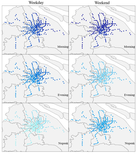
Figure 1.
Distribution of the Impact of Transportation service (darker colors indicate a greater degree of their influence).
Food & Beverages includes Chinese food restaurants, foreign food restaurants, fast food restaurants, coffee houses, dessert houses, and similar establishments. The coefficients of the variables for different time periods are shown in Figure 2, with darker colors indicating a greater degree of their influence. The impact on weekdays is significantly higher than that on non-weekdays, possibly because there are usually more dining options near metro stations. People often choose nearby dining establishments to save commuting time, thereby contributing to increased metro ridership.
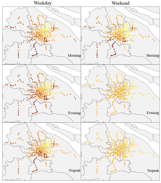
Figure 2.
Distribution of the Impact of Food & Beverages (darker colors indicate a greater degree of their influence).
Sports & Recreation have a negative impact on metro ridership. Places such as sports stadiums, recreation centers, theaters, and cinemas are not typically located near metro stations. People usually choose to drive or walk when going to these venues, which does not contribute to an increase in metro ridership.
Population density has a positive impact on metro ridership. The greater the population density, the higher the demand for residents to travel, thus promoting an increase in metro ridership.
The impact of Commercial & Industrial places is shown in Figure 3, with darker colors indicating a greater degree of their influence. Commercial & Industrial places have a positive impact on metro ridership, with a higher impact on weekdays than on non-weekdays, and a greater impact in the northeast compared to the southwest (Figure 3). Commercial and industrial areas typically concentrate numerous businesses and office spaces, attracting a large number of employees to work in these areas. The metro system, as a fast and efficient commuting option, provides convenient transportation services, helping employees reach their workplaces and return home quickly, thereby increasing metro ridership.
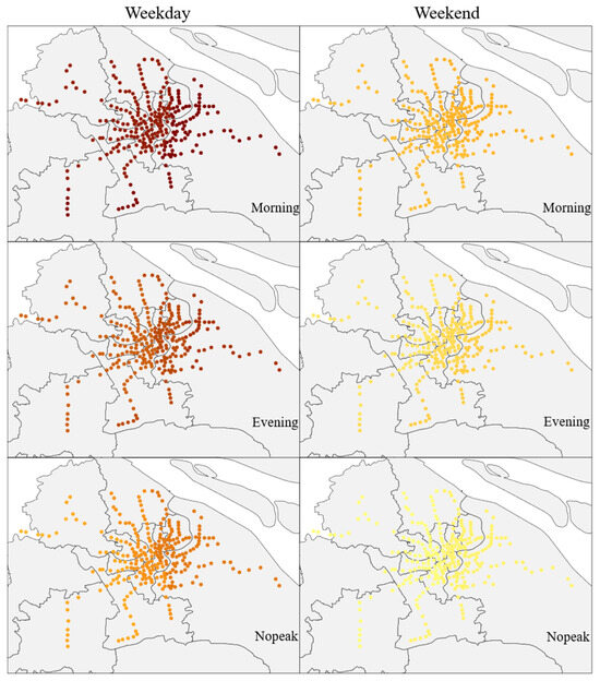
Figure 3.
Distribution of the Impact of Commercial & Industrial places (darker colors indicate a greater degree of their influence).
Government agencies mainly include government offices, public security and judicial agencies, industrial and commercial tax authorities, etc., typically serving as workplaces for government personnel, resulting in an overall negative impact on metro ridership.
Accommodation services have an overall positive impact on metro ridership. The more hotels, guesthouses, and similar establishments are distributed, the greater the metro ridership. Since those in need of accommodation services are often travelers from out of town or business professionals, considering the need for public transportation, they tend to choose hotels located near metro stations, thereby increasing metro ridership. In terms of temporal and spatial distribution, the impact on non-weekdays is noticeably higher than on weekdays, with the impact gradually increasing from north to south (Figure 4).
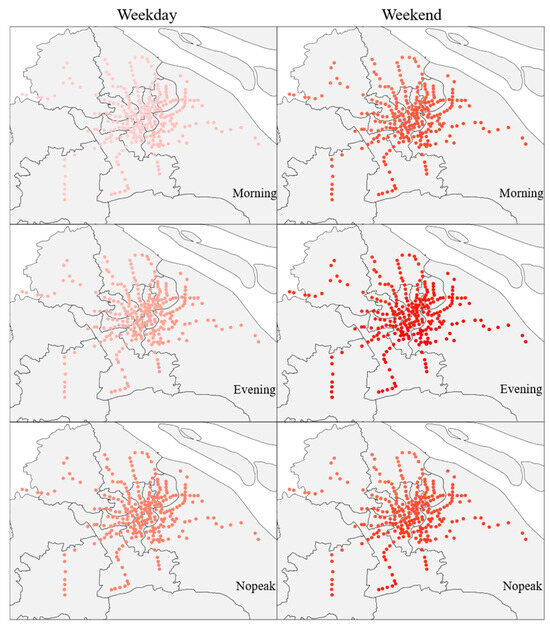
Figure 4.
Distribution of the Impact of Accommodation services (darker colors indicate a greater degree of their influence).
Scenic spots have a positive impact on metro ridership. Tourist attractions typically attract a large number of visitors and are often located around metro stations. As a convenient mode of transportation, the metro can efficiently transport tourists directly to their destinations, attracting more people to choose the metro to travel to scenic spots, thereby increasing metro ridership. In terms of time distribution, the impact of non-working days is greater than that of working days, with the least impact during the morning rush hour period. This is because people typically visit tourist attractions during non-working hours, indicating a relatively active leisure lifestyle in Shanghai [11]. In terms of spatial distribution, the impact gradually strengthens from south to north.
Land use diversity has an overall positive impact on metro ridership [5]. The greater the diversity in land use, with multiple functional zones indicating the presence of commercial, office, residential, cultural, tourism, educational, and other various types of areas, the metro, as a convenient and efficient mode of public transportation, can meet the travel needs of different groups, thereby promoting an increase in metro ridership.
Road density has a positive impact on metro ridership, indicating that a well-connected street network with convenient pathways can increase the number of metro passengers. Existing research has also confirmed this relationship [6]. A higher road network density indicates a well-developed road network in the area, connecting multiple functional zones and possibly being positioned as a transportation hub that attracts residents. Additionally, the transportation environment in the area is complex, with a significant volume of traffic, leading to prominent issues of vehicle congestion. Residents tend to prefer the timely and efficient metro as their mode of transportation in such areas.
5.4. The Interaction Influence of Factors
By using factor analysis, an analysis was conducted on the impact of various variables on metro ridership changes during different time periods. Figure 5 compares the q-values of different environmental variables during weekdays and weekends at different time periods. From the graph, it is evident that there are differences in the q-values of different environmental variables during various time periods. Apart from Road density, most variables have the highest q-values during off-peak hours and the lowest q-values during peak hours.
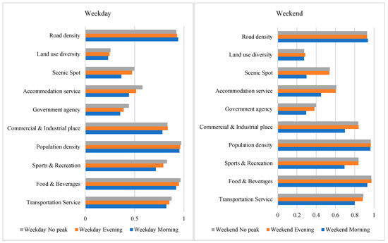
Figure 5.
Distribution of q-values for each variable at different time periods.
Furthermore, the q-values of the single-factor impact levels of road density, population density, and food & beverages all exceed 0.9, making them some of the variables with the greatest impact on changes in metro ridership. To facilitate subsequent analysis of two-factor impact levels, these variables will be excluded.
Interactions detectors are used to check whether two influencing factors work independently and further determine the type of interaction. This method has been applied in detecting influencing factors in traffic accidents research [44]. It was found that all factors mutually reinforce each other to increase their impact on metro ridership, involving two types of interactions: nonlinear enhancement and bi-enhancement. When any two factors work together, their combined explanatory power on metro ridership is greater than that of individual factors.
In terms of explanatory power ranking, the details of the top three interaction effects during each time period are shown in Table 7. It was observed that the factors with influence exceeding 0.7 in univariate analysis are transportation service, commercial & industrial place, and sports & recreation in Table 7. The strongest explanations in bivariate interaction effects come from interactions between three main factors and other factors. Specifically, while the univariate impact of Land use diversity does not exceed 0.3, indicating it is insignificantly influential on metro ridership, its impact level reaches 0.99 when interacting with main factors.
Table 7.
The Interactive Detector Results.
Furthermore, in the context of bivariate interaction effects across six distinct time intervals, the majority manifest bi-enhancement proclivities, where the cumulative impact surpasses the maximum individual factor impact. Concurrently, interactions involving Land use diversity and other factors, namely Government agency, Accommodation Service, and Scenic Spot, all adopt nonlinear enhancement characteristics. It significantly escalates the combined explanatory prowess in such scenarios. The interaction effects revealed by GeoDetector analysis provide actionable insights for integrated urban planning. The synergistic enhancement between land use diversity and other factors suggests that mixed-use development policies should be implemented as part of comprehensive packages rather than isolated interventions. For instance, when developing new metro stations, simultaneously introducing diverse commercial facilities, improving road connectivity, and ensuring adequate public service provisions can generate multiplicative effects on ridership. This finding challenges the conventional single-factor optimization approach and advocates for coordinated multi-sectoral planning strategies. Urban planners should leverage these interaction effects by creating policy bundles that combine transportation infrastructure investments with targeted land use regulations and public facility allocations, thereby maximizing the return on public transit investments.
6. Conclusions
Based on the case study of Shanghai, this research investigates the impact of BE factors on metro ridership. We employed the MGWR model with a more flexible bandwidth setting to analyze spatial heterogeneity of BE on metro ridership. By comparing the modeling results with GWR and OLS models, we validated the potential application value of the MGWR model in analyzing factors influencing rail transit ridership. The analysis of single-factor effects on rail transit ridership indicates that variables such as Transportation Service, Food & Beverages, Population Density, Commercial & Industrial Places, Accommodation Service, and Scenic Spots all have a positive impact. Particularly, Food & Beverages and Accommodation services, respectively, have the greatest impact on metro ridership on weekday and weekend. Considering limited resources and feasibility of construction, it could be beneficial to increase connectivity by strategically locating transportation hubs near metro stations. Placing malls, office buildings, and other commercial establishments near metro stations can also boost rail transit ridership.
Following single-factor analysis, the GeoDetector was utilized to analyze the interactive effects of built environment factors. The findings revealed a significant improvement in explanatory power with the consideration of bivariate interaction effects. The results from the analysis of bivariate interaction effects reveal that in conjunction with Land Use Diversity and other variables, there is a significant enhancement in the impact on rail transit ridership. Thus, it is recommended to diversify land use near metro stations by implementing incentive measures to encourage the development of mixed-use buildings. This approach can create a diverse environment that caters to various needs and contributes to increasing rail transit ridership.
This study holds significant implications for sustainable urban development. The findings indicate that the metro ridership in central urban areas is primarily driven by commercial density, while suburban ridership is more sensitive to accessibility of public services. This necessitates differentiated policy interventions—prioritizing the allocation of hospitals, schools, and other essential facilities near suburban stations to mitigate spatial deprivation of public services. In addition, these research findings demonstrate that coordinated planning of transportation hubs and commercial facilities can increase the share of rail-based travel. By optimizing mixed-use development within an 800 m radius around metro stations (e.g., transit-oriented development (TOD) models), reliance on private vehicles for short-distance trips can be reduced.
Current limitations in data sources may introduce potential biases related to variable types and temporal coverage. While the 2016 data used in this study, the fundamental relationships between built environment characteristics and transit ridership patterns tend to remain stable over medium-term periods. Shanghai’s metro network expansion since 2016 has primarily occurred in peripheral areas, while the core network analyzed in this study has remained largely unchanged. Furthermore, the methodological framework we present—combining MGWR with GeoDetector for interaction analysis—remains valid and can be readily applied to more recent datasets as they become available. In future research, we aim to acquire a more diverse and comprehensive set of data variables to further refine our models. This will allow us to explore the factors influencing rail transit ridership more comprehensively and deeply, providing valuable insights and recommendations for sustainable transportation development.
Author Contributions
Conceptualization, Q.X. and Y.P.; methodology, Q.X. and L.C.; software, L.C. and Z.L.; validation, L.C., H.W. and Z.L.; formal analysis, H.W. and H.L.; investigation, H.L. and Y.P.; resources, Y.X.; data curation, Y.X.; writing—original draft preparation, L.C. and Z.L.; writing—review and editing, H.W. and H.L.; visualization, L.C. and Z.L.; supervision, Y.X. and Y.P.; project administration, Y.P.; funding acquisition, Q.X. and Y.X. All authors have read and agreed to the published version of the manuscript.
Funding
This research was funded by Natural Science Foundation of Jiangsu Province (BK20230893), Natural Science Foundation of Shanghai (22ZR1465500), and the National Natural Science Foundation of China (52302440).
Institutional Review Board Statement
Not applicable.
Informed Consent Statement
Not applicable.
Data Availability Statement
The raw data supporting the conclusions of this article will be made available by the authors on request.
Conflicts of Interest
The authors declare no conflict of interest.
References
- Ding, H.; Zhao, Z.; Wang, S.; Zhang, Y.; Zheng, X.; Lu, X. Quantifying the Impact of Built Environment on Traffic Congestion: A Nonlinear Analysis and Optimization Strategy for Sustainable Urban Planning. Sustain. Cities Soc. 2025, 122, 106249. [Google Scholar] [CrossRef]
- Li, S.; Liu, X.; Li, Z.; Wu, Z.; Yan, Z.; Chen, Y.; Gao, F. Spatial and Temporal Dynamics of Urban Expansion Along the Guangzhou–Foshan Inter-City Rail Transit Corridor, China. Sustainability 2018, 10, 593. [Google Scholar] [CrossRef]
- Zhao, J.; Deng, W.; Song, Y.; Zhu, Y. What Influences Metro Station Ridership in China? Insights from Nanjing. Cities 2013, 35, 114–124. [Google Scholar] [CrossRef]
- Lu, K.; Zhang, L.; Li, S.; Huang, Y.; Ding, X.; Hao, J.; Huang, S.; Li, X.; Lu, F.; Zhang, H. Urban Rail Transit in China: Progress Report and Analysis (2015–2023). Urban Rail Transit 2025, 11, 1–27. [Google Scholar] [CrossRef]
- Li, S.; Lyu, D.; Liu, X.; Tan, Z.; Gao, F.; Huang, G.; Wu, Z. The Varying Patterns of Rail Transit Ridership and Their Relationships with Fine-Scale Built Environment Factors: Big Data Analytics from Guangzhou. Cities 2020, 99, 102580. [Google Scholar] [CrossRef]
- Liu, M.; Liu, Y.; Ye, Y. Nonlinear Effects of Built Environment Features on Metro Ridership: An Integrated Exploration with Machine Learning Considering Spatial Heterogeneity. Sustain. Cities Soc. 2023, 95, 104613. [Google Scholar] [CrossRef]
- Jun, M.-J.; Choi, K.; Jeong, J.-E.; Kwon, K.-H.; Kim, H.-J. Land Use Characteristics of Subway Catchment Areas and Their Influence on Subway Ridership in Seoul. J. Transp. Geogr. 2015, 48, 30–40. [Google Scholar] [CrossRef]
- Gutiérrez, J.; Cardozo, O.D.; García-Palomares, J.C. Transit Ridership Forecasting at Station Level: An Approach Based on Distance-Decay Weighted Regression. J. Transp. Geogr. 2011, 19, 1081–1092. [Google Scholar] [CrossRef]
- Ryan, S.; Frank, L.F. Pedestrian Environments and Transit Ridership. J. Public Transp. 2009, 12, 39–57. [Google Scholar] [CrossRef]
- Sun, L.-S.; Wang, S.-W.; Yao, L.-Y.; Rong, J.; Ma, J.-M. Estimation of Transit Ridership Based on Spatial Analysis and Precise Land Use Data. Transp. Lett. 2016, 8, 140–147. [Google Scholar] [CrossRef]
- An, D.; Tong, X.; Liu, K.; Chan, E.H. Understanding the Impact of Built Environment on Metro Ridership Using Open Source in Shanghai. Cities 2019, 93, 177–187. [Google Scholar] [CrossRef]
- Tobler, W.R. A Computer Movie Simulating Urban Growth in the Detroit Region. Econ. Geogr. 1970, 46, 234–240. [Google Scholar] [CrossRef]
- Blainey, S. Trip End Models of Local Rail Demand in England and Wales. J. Transp. Geogr. 2010, 18, 153–165. [Google Scholar] [CrossRef]
- An, R.; Wu, Z.; Tong, Z.; Qin, S.; Zhu, Y.; Liu, Y. How the Built Environment Promotes Public Transportation in Wuhan: A Multiscale Geographically Weighted Regression Analysis. Travel Behav. Soc. 2022, 29, 186–199. [Google Scholar] [CrossRef]
- Li, M.; Kwan, M.-P.; Hu, W.; Li, R.; Wang, J. Examining the Effects of Station-Level Factors on Metro Ridership Using Multiscale Geographically Weighted Regression. J. Transp. Geogr. 2023, 113, 103720. [Google Scholar] [CrossRef]
- Ding, C.; Liu, T.; Yao, B.; Zhang, Y.; Qiao, X. Understanding the Time-Dependent Effect of Built Environment Attributes on Station-Level Metro Ridership Uncertainty in Beijing: A Big Data Analytic Approach. Tunn. Undergr. Space Technol. 2023, 137, 105148. [Google Scholar] [CrossRef]
- Eom, J.K.; Choi, J.; Park, M.S.; Heo, T.-Y. Exploring the Catchment Area of an Urban Railway Station by Using Transit Card Data: Case Study in Seoul. Cities 2019, 95, 102364. [Google Scholar] [CrossRef]
- He, Y.; Zhao, Y.; Tsui, K.L. Modeling and Analyzing Impact Factors of Metro Station Ridership: An Approach Based on a General Estimating Equation. IEEE Intell. Transp. Syst. Mag. 2020, 12, 195–207. [Google Scholar] [CrossRef]
- Merlin, L.A.; Singer, M.; Levine, J. Influences on Transit Ridership and Transit Accessibility in US Urban Areas. Transp. Res. Part A Policy Pract. 2021, 150, 63–73. [Google Scholar] [CrossRef]
- Wang, Z.; Song, J.; Zhang, Y.; Li, S.; Jia, J.; Song, C. Spatial Heterogeneity Analysis for Influencing Factors of Outbound Ridership of Subway Stations Considering the Optimal Scale Range of “7D” Built Environments. Sustainability 2022, 14, 16314. [Google Scholar] [CrossRef]
- Zhou, X.; Yeh, A.G.; Yue, Y. Spatial Variation of Self-Containment and Jobs-Housing Balance in Shenzhen Using Cellphone Big Data. J. Transp. Geogr. 2018, 68, 102–108. [Google Scholar] [CrossRef]
- Song, Y.; Huang, B.; He, Q.; Chen, B.; Wei, J.; Mahmood, R. Dynamic Assessment of PM2.5 Exposure and Health Risk Using Remote Sensing and Geo-Spatial Big Data. Environ. Pollut. 2019, 253, 288–296. [Google Scholar] [CrossRef] [PubMed]
- Li, X.Y.; Sinniah, G.K.; Li, R. Identify Impacting Factor for Urban Rail Ridership from Built Environment Spatial Heterogeneity. Case Stud. Transp. Policy 2022, 10, 1159–1171. [Google Scholar] [CrossRef]
- Shi, Z.; Zhang, N.; Liu, Y.; Xu, W. Exploring Spatiotemporal Variation in Hourly Metro Ridership at Station Level: The Influence of Built Environment and Topological Structure. Sustainability 2018, 10, 4564. [Google Scholar] [CrossRef]
- Gan, Z.; Yang, M.; Feng, T.; Timmermans, H.J. Examining the Relationship Between Built Environment and Metro Ridership at Station-to-Station Level. Transp. Res. Part D Transp. Environ. 2020, 82, 102332. [Google Scholar] [CrossRef]
- Chen, E.; Ye, Z.; Wang, C.; Zhang, W. Discovering the Spatio-Temporal Impacts of Built Environment on Metro Ridership Using Smart Card Data. Cities 2019, 95, 102359. [Google Scholar] [CrossRef]
- Fu, X.; Zhao, X.X.; Li, C.C.; Cui, M.Y.; Wang, J.W.; Qiang, Y.J. Exploration of the Spatiotemporal Heterogeneity of Metro Ridership Prompted by Built Environment: A Multi-Source Fusion Perspective. IET Intell. Transp. Syst. 2022, 16, 1455–1470. [Google Scholar] [CrossRef]
- Wang, J.; Wan, F.; Dong, C.; Yin, C.; Chen, X. Spatiotemporal Effects of Built Environment Factors on Varying Rail Transit Station Ridership Patterns. J. Transp. Geogr. 2023, 109, 103597. [Google Scholar] [CrossRef]
- Kim, D.; Ahn, Y.; Choi, S.; Kim, K. Sustainable Mobility: Longitudinal Analysis of Built Environment on Transit Ridership. Sustainability 2016, 8, 1016. [Google Scholar] [CrossRef]
- Tu, W.; Cao, R.; Yue, Y.; Zhou, B.; Li, Q.; Li, Q. Spatial Variations in Urban Public Ridership Derived from GPS Trajectories and Smart Card Data. J. Transp. Geogr. 2018, 69, 45–57. [Google Scholar] [CrossRef]
- Li, X. Analysis of Taxi Demand and Traffic Influencing Factors in Urban Core Area Based on Data Field Theory and GWR Model: A Case Study of Beijing. Sustainability 2024, 16, 7386. [Google Scholar] [CrossRef]
- Huang, B.; Wu, B.; Barry, M. Geographically and Temporally Weighted Regression for Modeling Spatio-Temporal Variation in House Prices. Int. J. Geogr. Inf. Sci. 2010, 24, 383–401. [Google Scholar] [CrossRef]
- Lessani, M.; Li, Z. SGWR: Similarity and Geographically Weighted Regression. Int. J. Geogr. Inf. Sci. 2024, 38, 1232–1255. [Google Scholar] [CrossRef]
- Fotheringham, A.S.; Yang, W.; Kang, W. Multiscale Geographically Weighted Regression (MGWR). Ann. Am. Assoc. Geogr. 2017, 107, 1247–1265. [Google Scholar] [CrossRef]
- Yu, H.; Fotheringham, A.S.; Li, Z.; Oshan, T.; Kang, W.; Wolf, L.J. Inference in Multiscale Geographically Weighted Regression. Geogr. Anal. 2020, 52, 87–106. [Google Scholar] [CrossRef]
- Wang, J.-F.; Zhang, T.-L.; Fu, B.-J. A Measure of Spatial Stratified Heterogeneity. Ecol. Indic. 2016, 67, 250–256. [Google Scholar] [CrossRef]
- Qiao, P.; Yang, S.; Lei, M.; Chen, T.; Dong, N. Quantitative Analysis of the Factors Influencing Spatial Distribution of Soil Heavy Metals Based on Geographical Detector. Sci. Total Environ. 2019, 664, 392–413. [Google Scholar] [CrossRef]
- Peng, W.; Kuang, T.; Tao, S. Quantifying Influences of Natural Factors on Vegetation NDVI Changes Based on Geographical Detector in Sichuan, Western China. J. Clean. Prod. 2019, 233, 353–367. [Google Scholar] [CrossRef]
- Peng, W.; Fan, Z.; Duan, J.; Gao, W.; Wang, R.; Liu, N.; Hua, S. Assessment of Interactions Between Influencing Factors on City Shrinkage Based on Geographical Detector: A Case Study in Kitakyushu, Japan. Cities 2022, 131, 103958. [Google Scholar] [CrossRef]
- Wang, Y.; Wang, S.; Li, G.; Zhang, H.; Jin, L.; Su, Y.; Wu, K. Identifying the Determinants of Housing Prices in China Using Spatial Regression and the Geographical Detector Technique. Appl. Geogr. 2017, 79, 26–36. [Google Scholar] [CrossRef]
- Wang, J.F.; Li, X.H.; Christakos, G.; Liao, Y.L.; Zhang, T.; Gu, X.; Zheng, X.Y. Geographical Detectors-Based Health Risk Assessment and Its Application in the Neural Tube Defects Study of the Heshun Region, China. Int. J. Geogr. Inf. Sci. 2010, 24, 107–127. [Google Scholar] [CrossRef]
- Pan, H.; Li, J.; Shen, Q.; Shi, C. What Determines Rail Transit Passenger Volume? Implications for Transit Oriented Development Planning. Transp. Res. Part D Transp. Environ. 2017, 57, 52–63. [Google Scholar] [CrossRef]
- Li, S.; Lyu, D.; Huang, G.; Zhang, X.; Gao, F.; Chen, Y.; Liu, X. Spatially Varying Impacts of Built Environment Factors on Rail Transit Ridership at Station Level: A Case Study in Guangzhou, China. J. Transp. Geogr. 2020, 82, 102631. [Google Scholar] [CrossRef]
- Zhang, Y.; Lu, H.; Qu, W. Geographical Detection of Traffic Accidents Spatial Stratified Heterogeneity and Influence Factors. Int. J. Environ. Res. Public Health 2020, 17, 572. [Google Scholar] [CrossRef] [PubMed]


Disclaimer/Publisher’s Note: The statements, opinions and data contained in all publications are solely those of the individual author(s) and contributor(s) and not of MDPI and/or the editor(s). MDPI and/or the editor(s) disclaim responsibility for any injury to people or property resulting from any ideas, methods, instructions or products referred to in the content. |
© 2025 by the authors. Licensee MDPI, Basel, Switzerland. This article is an open access article distributed under the terms and conditions of the Creative Commons Attribution (CC BY) license (https://creativecommons.org/licenses/by/4.0/).