Article

Modelling the Cyclical Variability of Nitrogen Dioxide in Urban Areas of Poland, 2001–2021

by
Szymon Ignaciuk
,
Dorota Domagała
* and
Małgorzata Szczepanik
*
Department of Applied Mathematics and Computer Science, University of Life Sciences in Lublin, ul. Akademicka 13, 20-950 Lublin, Poland
*
Authors to whom correspondence should be addressed.
Sustainability 2025, 17(21), 9456; https://doi.org/10.3390/su17219456 (registering DOI)
Submission received: 7 July 2025 / Revised: 2 October 2025 / Accepted: 17 October 2025 / Published: 24 October 2025
(This article belongs to the Section Air, Climate Change and Sustainability)

Abstract

High concentrations of NO2 in the air have a negative impact on human health, increasing the risk of cardiovascular diseases such as heart attacks and strokes, as well as causing pulmonary oedema and weak heartbeat. The aim of this study was to develop a mathematical model describing the cyclical variability of NO2 concentrations, which is crucial for risk assessment and preventive action planning. Based on long-term data from 47 measuring stations located throughout Poland, the sum of sines model was fitted, which reflected seasonal and cyclical fluctuations in NO2 concentrations and allowed the identification of periods with the highest NO2 values, especially in winter months and during traffic peaks. The results can be used to support environmental policy and decision-making on preventive measures, for example, related to traffic restrictions, as well as in sustainable urban planning and in the protection of public health and the environment, thereby contributing to the achievement of global sustainable development goals.

1. Introduction

Air pollution has a negative impact on human health and well-being [1,2,3,4,5,6,7] and adversely affects the environment: climate, water, soil, plants and animals [8,9]. It is a global phenomenon and, as such, constitutes a serious problem. Pollution is the result of natural processes such as forest fires, volcanic eruptions and human activities related to, among other things, road transport, fuels and energy production. Air pollution consists mainly of dust, carbon oxides, sulphur dioxide, hydrogen sulphide, fluorine, nitrogen oxides, hydrogen compounds and aromatic hydrocarbons. According to the WHO, environmental stress factors are responsible for 15–20% of all deaths in European countries, whereas the OECD notes that by 2050, pollution levels in cities will be the main cause of mortality worldwide [10]. This is not encouraging, especially since it is predicted that by that time the percentage of the population living in cities will increase to around 70% [11,12]. A nine-year-old Ella Adoo-Kissi-Debrah, the first person in the world whose death was officially attributed to air pollution in 2021, has become a symbol of the toxic impact of air pollution on human life [13]. The negative influence of air pollution on human health is also reflected in the economic situation, causing a decrease in worker productivity, an increase in healthcare costs and a reduction in life expectancy [14]. Particulate matter PM10 and PM2.5, nitrogen dioxide NO2 and ozone O3 are considered to be the most harmful to human health [14].
Much attention has been paid to particulate matter, which is responsible for the exacerbation of symptoms of respiratory diseases (asthma, weakened lung function, acute bronchitis) and cardiovascular diseases (vasculitis, atherosclerosis) as well as lung, larynx and throat cancer [3,5]. Moreover, they indirectly increase the risk of heart attack and stroke [15,16,17,18,19,20,21,22,23,24,25,26]. Thurston et al. have identified a link between excessive exposure to PMx and Alzheimer’s and Parkinson’s disease [27]. However, protection against particulate matter is possible. When particulate matter concentration limits are exceeded, it is recommended to limit outdoor activities and use good-quality anti-smog masks, and use air purifiers with the appropriate type of filter in closed rooms. To provide one of the examples, HEPA filters are capable of eliminating PMx particles with over 99% efficiency [28,29], but they are not able to stop gaseous pollutants.
One of the most dangerous air pollutants, particularly detrimental to human health, is nitrogen dioxide. NO2 at a concentration of 0.12 µg/dm3 irritates the mucous membranes of the upper respiratory tract, and at a concentration of 0.19 µg/dm3 causes coughing. NO2 in high concentrations has a narcotic effect, causes pulmonary oedema, weakens the heartbeat, has a negative impact on the heart and circulatory system, increasing the risk of cardiovascular diseases such as heart attack and stroke. In chronic NO2 poisoning, inflammation, conjunctival irritation and mouth ulcers occur [14,15,30,31,32].
Nitrogen dioxide has a pungent odour and brown colour, which gives smog its characteristic colour. The presence of nitrogen dioxide in the atmosphere is influenced by natural factors such as volcanic eruptions, electrostatic discharges and the activity of microorganisms, as well as factors related to human activity. Natural sources of nitrogen dioxide emissions are distributed across the entire surface of the Earth, and the resulting NO2 content in the air is very low. Nitrogen dioxide comes largely from various combustion processes, for example in electricity and cement production [33], in metallurgy, in domestic heating [34]—in some areas, a large number of houses are heated with coal, natural gas or fuel oil boilers. Agriculture is also a significant source of emissions through the use of nitrogen fertilisers [35], which can emit nitrogen oxides as a result of biological processes. However, road transport, especially diesel engines, is mainly responsible for NO2 emissions. In Poland, road transport accounts for 35% of nitrogen oxide emissions (37% in Europe), 21% is caused by energy production (14% in Europe), 20% by agriculture (19% in Europe), and 22% by industry and the municipal sector (24% in Europe) [32,36].
Since 2015, the EURO 6 standard has been implemented in Europe, setting maximum permissible levels of vehicle emissions for both petrol and diesel engines. Compared to the EURO 3 standard implemented since 2000, it provides for a 2.5-fold reduction in nitrogen oxide emissions from petrol engines and a 7.5-fold reduction from diesel engines in newly registered vehicles [37]. Reducing the negative influence of transport on the environment is one of the objectives of the European Union’s transport policy.
Poland has one of the oldest car fleets in Europe [38], which means higher NOx and CO2 emissions [39,40]. Based on the data on passenger cars published in the Central Vehicles and Drivers Register [41], there can be observed a steady increase in their number between 2001 and 2010, from approximately 10 million registered vehicles in 2001 to approximately 18 million in 2010. Undoubtedly, Poland’s accession to the European Union in 2004 played a significant role in this trend, as it led to a sharp increase in imports of used cars from Western European countries. The abolition of customs duties, many import restrictions and the simplification of procedures meant that in the first years after the accession, hundreds of thousands of imported vehicles were registered every year. This also contributed to a decline in the prices of used cars in Poland. Initially, relatively new cars were imported, but subsequently, the age of imported cars increased, averaging 10–12 years. After 2010, the growth in the number of registered passenger cars slowed down, reaching approximately 24 million at the end of 2021, with an estimated 19–20 million vehicles actually in use [41,42]. Between 2001 and 2010, due to cheap imports from Western Europe, the percentage of diesel cars grew dynamically, reaching around 40–43% in 2010-16. In the following years, this percentage demonstrated a downward trend, reaching around 38–40% in 2021. This was influenced, among other things, by the Euro 6d emission standards and increasingly expensive DPF/AdBlue filters, as well as plans to introduce clean transport zones and subsidies for the purchase of electric cars. In 2021, Poland had the highest percentage of passenger cars older than 20 years in the EU (41.3%), cars aged 10–20 years accounted for 37.1%, and new cars up to 2 years old accounted for less than 5%. The average age of passenger cars in Poland is approximately 14.1–14.6 years, compared to 11.8–12 years in the EU [38]. In 2018, excise duty rules were changed to reward younger cars. EU regulations provide for the phasing out of combustion engines in newly registered cars by 2035 [43]. As an EU member state, Poland is obliged to reduce emissions from transport, but the high proportion of old cars makes it much more difficult to achieve the climate improvement target.
Between 2005 and 2021, both Poland and Europe had fixed standards for permissible air pollution concentrations, in line with WHO guidelines. For nitrogen dioxide, the average hourly limit value was 200 µg/m3 with a limit of 18 exceedances per year, while the average annual value should not exceed 40 µg/m3 [44,45,46]. Due to the negative impact of air pollution on human health, in 2021, the WHO recommended tightening these standards [47]. Therefore, for nitrogen dioxide, the annual average was reduced fourfold and should not exceed 10 µg/m3, while the hourly average was maintained at 200 µg/m3. When a 24-h value of 25 µg/m3 was introduced for the first time, it was recognised as a safe level for short-term exposure. The WHO guidelines are not legally binding, but they are the most rigorous scientific recommendations for the protection of public health.
Many Polish cities are frequently viewed as the most polluted places in Europe [48,49]. Therefore, it is extremely important to monitor air quality, which provides information on pollution levels, exceedances and the effectiveness of socio-economic programmes aimed at improving the environment.
In Poland, air pollution concentrations are monitored by the Chief Inspectorate for Environmental Protection and its regional branches. The air quality monitoring system in the province is defined by provincial environmental monitoring programmes developed by the Regional Environmental Monitoring Departments. This system is based on a network of measuring stations located at critical points in the province, mainly in cities where analyses demonstrate high concentrations of pollutants. The criteria for the location of measuring stations are specified in the Regulation of the Minister of the Environment of 11 December 2020 on the assessment of air pollutant levels. The Chief Inspectorate for Environmental Protection is responsible for the station measurement programme (location, number of stations, their measurement range), which is based on long-term air quality assessments in accordance with Article 88 [2] of the Act of 27 November 2001—Environmental Protection Law. Measurements are carried out continuously at pollution monitoring stations. Every hour, the so-called instantaneous concentrations are recorded, which are, in fact, average values for a period of one hour. In the vast majority of measuring stations in Poland, measurements are performed automatically, but there are also stations where measurements are taken manually. These measurements are highly accurate and have low uncertainty, but their disadvantage is their high cost and low spatial density. There are 291 measuring stations in Poland, of which 218 are automatic or automatic–manual [50].
The method for measuring nitrogen dioxide concentrations used in automatic monitoring in Poland, recognised by the European Commission as the reference method, is specified in standard PN-EN 14211:2013-02 [51]. This method is based on the phenomenon of chemiluminescence, i.e., the emission of light waves produced as a result of specific chemical reactions. Nitrogen oxide reacts in the gas phase with ozone to produce an excited, unstable nitrogen dioxide molecule. When this molecule returns to its ground state, it emits radiation in the wavelength range of 600–3000 nm. The intensity of the radiation is directly proportional to the concentration of nitrogen oxide. The concentration of nitrogen dioxide can only be measured after it has been converted to nitrogen oxide.
The aim of the study was to analyse the cyclical variation of nitrogen dioxide concentrations in the air as a function of time and to develop an adequate mathematical model to describe this variation in urban areas in Poland in the years 2001–2021. Urban environments are characterized by elevated vehicular density and traffic intensity within spatially constrained areas, conditions that substantially enhance anthropogenic nitrogen dioxide emissions and contribute to increased ambient concentrations of this pollutant. It should be noted that a large part of the urban area is covered by roads, most of which are asphalted, which, according to recent studies [11], is an additional source of NO2 emissions.
In view of growing challenges related to environmental protection, climate change, and the need to develop sustainable solutions, understanding the cyclical patterns of NO2 concentrations appears to be crucial for shaping policies that support sustainable urban mobility, developing strategies for the effective allocation of resources for environmental protection, urban planning, and planning preventive measures related to public health protection. This will enable the achievement of global sustainability goals associated with clean air and resilient communities.

2. Materials and Methods

The data on nitrogen dioxide concentrations were obtained from 254 urban measuring stations between 2001 and 2021 [52]. Nitrogen dioxide concentration values were recorded from Monday, 1 January 2001, at 1 a.m. to Friday, 31 December 2021, at 12 p.m. After analysing the data for completeness, it was revealed that many stations had too few recorded measurements to be included in further analysis. Eventually, only 50 stations were included in the study, where the gaps represented only a small percentage of the total data. Thus, a maximum of 184,079 results were obtained from each station.
In order to segment the measuring stations in terms of nitrogen dioxide concentration levels, cluster analysis based on a distance matrix was used. The distance matrix was constructed as follows: an hourly measurement matrix M 50 × 184,079 = m i , j was determined for 50 measuring stations, where m i , j R NaN , is a measurement (or lack thereof, in the case of m i , j = NaN , NaN means a missing value) air pollution levels by NO2 expressed in units of µ g / m 3 . Based on matrix M, matrix L = l i , j 50 × 50 was determined as the sum of common results in time between stations, where
l i , j = k = 1 184,079 m k , i NaN     a n d     m k , j NaN
and then the matrix D = d i , j n × n of the average distance between the pollution values between i th and j th stations, where
d i , j = + ,     f o r l i , j < 1440 k = 1 , where   m k , i N a N     and     m k , j N a N 184,079 m k , i m k , j l i , j ,     f o r l i , j 1440
If a pair of stations (i,j) meets the condition l i , j < 1440 , it means that there are insufficient measurements (less than 1440 = 24 · 30 · 2 , i.e., 2 months) at the same time between these stations. In this case, we assign a distance + to the pair (i,j) (during the analysis, this value was replaced with a constant very high value). The matrix D is a non-negative definite matrix which contains non-negative values and zeros on the diagonal. In fact, it is not a distance matrix in the strict sense, but rather a pseudodistance matrix. Nevertheless, matrix D can still be applied for hierarchical clustering. The clustering was performed using three linkage methods: ‘single’, ‘complete’ and ‘average’. All three methods consistently produced the same outcome.
Two clusters were obtained: I—containing only three measuring stations that recorded very high concentrations of nitrogen dioxide, and II—containing the remaining 47 stations. This study focused on cluster II. The basic data for the measuring stations from cluster II is presented in Table 1.
Before proceeding to the stage of fitting the model to the data, the data was averaged. The arithmetic mean of the measurements from each hour was calculated from the stations containing measurements at that time. This resulted in a vector Y of averaged measurement data from each hour during the study period. y j = Y j denotes the average nitrogen dioxide pollution at the time of j 1,2 , , 184,079 measurement, expressed in units of [ μ g / m 3 ] .
The following models were fitted to the data:
  • Gaussian: k = 1 n a k exp x b k c k 2 for n 1,2 , , 8 , a k , b k , c k R
  • Polynomial: k = 1 n a k x k for n 1,2 , , 8 , a k R
  • Rational: k = 1 n a k x k k = 1 m b k x k for m , n 1,2 , , 5 , a k , b k R
  • Sum of sines: k = 1 n a k sin b k x + c k for n 1,2 , , 8 , a k , b k , c k R
The calculations were performed using custom scripts written in the Matlab R2024b and Python 3.13 programming environments.

3. Results

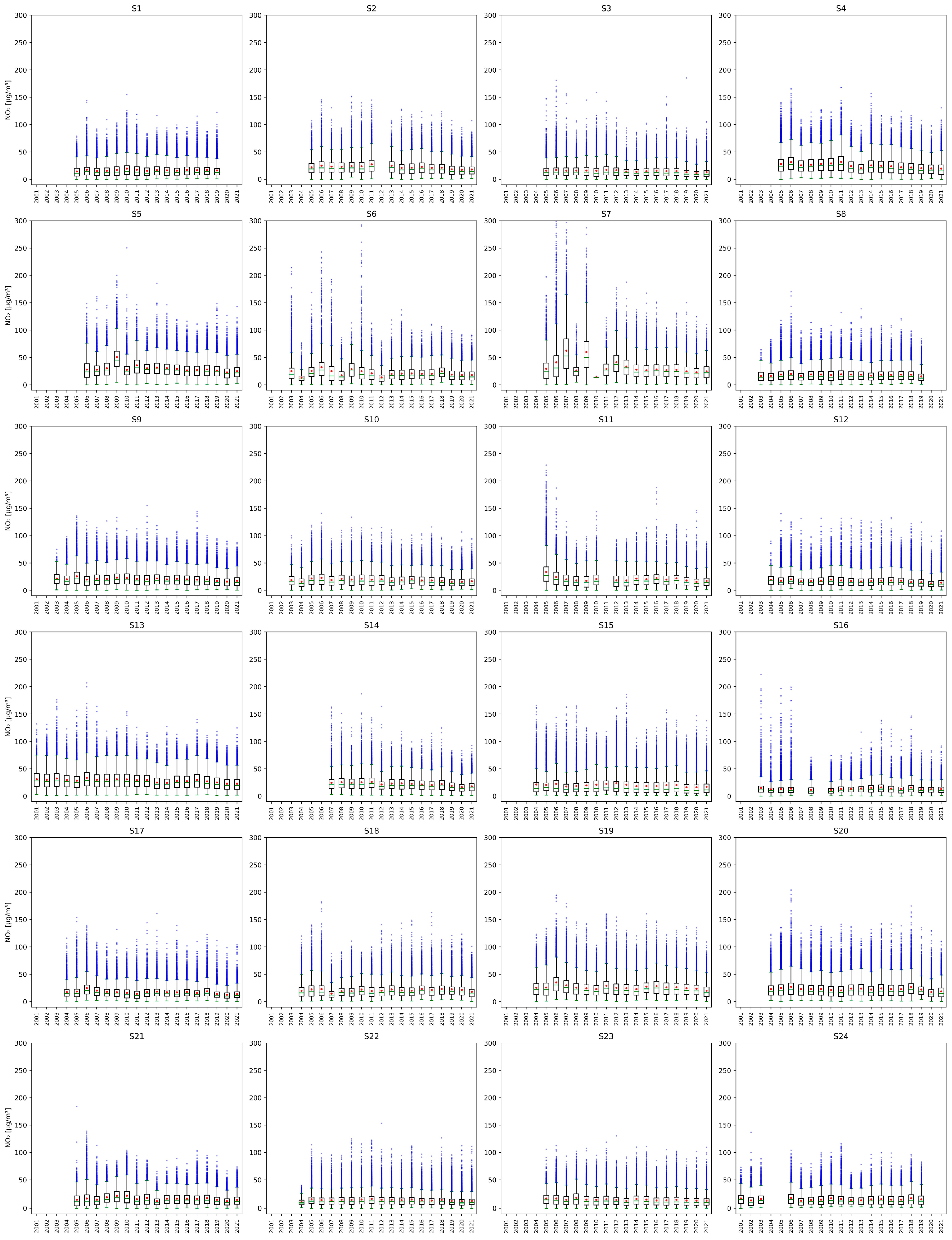
Between 2001 and 2021, nitrogen dioxide concentration trends were similar at most stations. In 2005, 17 stations reached their maximum average concentration. In 2006, as many as 39 stations recorded an increase in average nitrogen dioxide concentrations compared to the previous year, while in the following year, 40 stations recorded a decrease in average nitrogen dioxide concentrations, but the S7 station recorded a record value of over 62 µg/m3. The year 2009 also proved to be a year in which the limit value was significantly exceeded at two stations, S5 and S7. A similar situation occurred in 2012 (S2 and S7), but the average concentrations recorded only slightly exceeded 40 µg/m3. Since then, average annual concentrations have not demonstrated any radical increases, with declines at many stations. The year 2020 saw a marked decline in average concentrations, which was related to the COVID-19 pandemic and the most restrictive restrictions on leaving one’s place of residence and movement. However, in the following year, after many restrictions were lifted, average concentrations increased (Figure 1, Figure A1 and Figure A2).
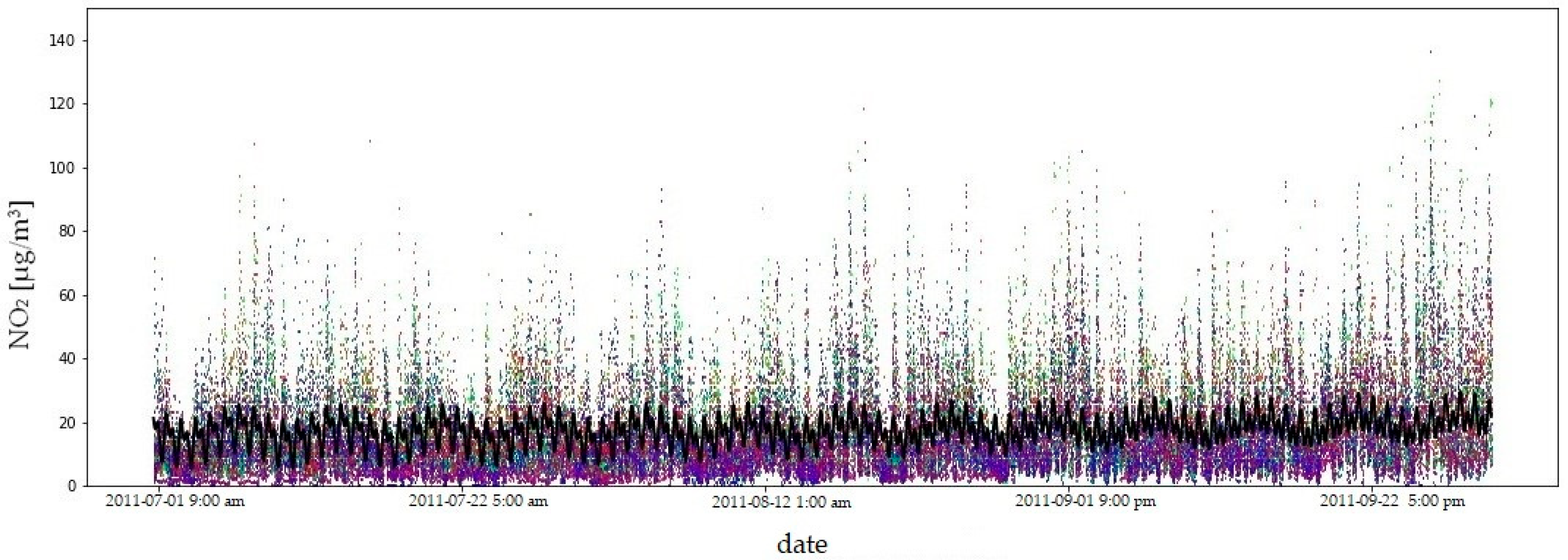
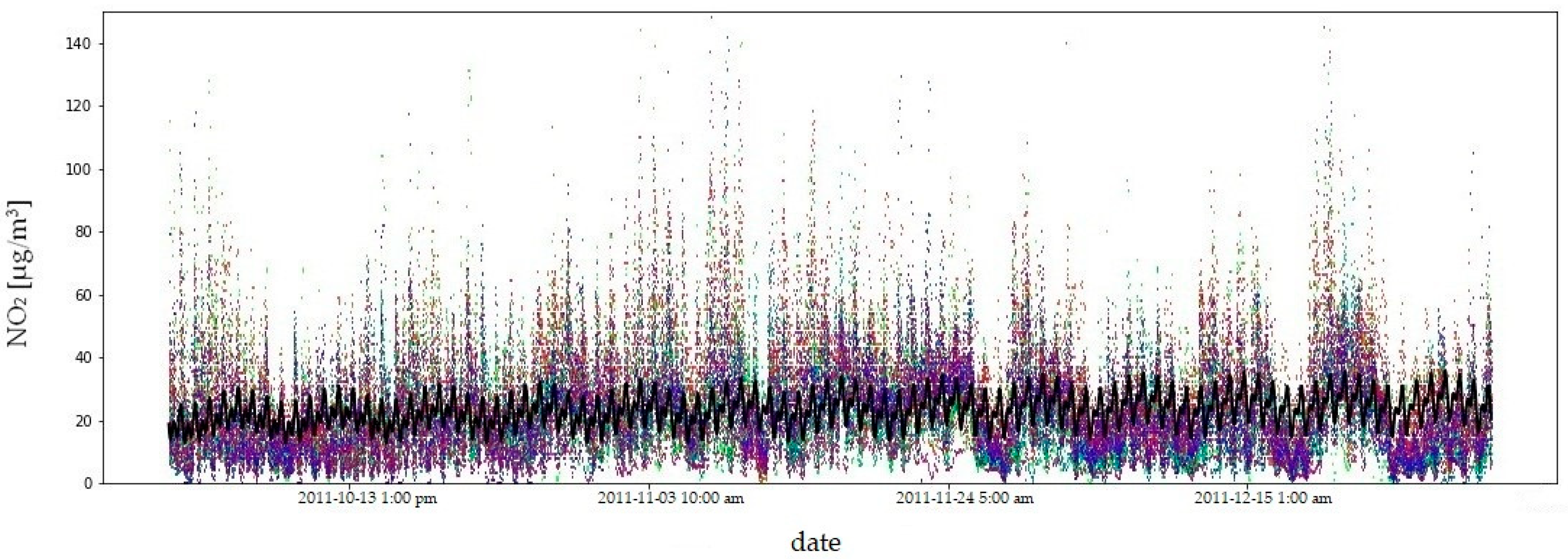
The goodness of fit of the model to the observed data was assessed using the coefficient of determination. The coefficients of determination ( R 2 ) for evaluated models—Gaussian, polynomial, rational and sum of sines—were 0.2997, 0.2764, 0.2598, and 0.3366, respectively. So, the best model (with the highest R 2 ) describing the variability of nitrogen dioxide concentration in the 47 stations studied is the sum of sines model consisting of eight components of the form:
S C x = a sin b x + c ,
a , b , c R for x from a certain range I .
Each of these components can be interpreted in two ways, depending on the value of the parameter b obtained, because the magnitude 2 π / b determines the period of the sine function:
  • If 2 π / b is (much) greater than the length of the range I , then the property sin ( x ) / x 1 for x 0 is used. In this case, S C behaves similarly to a linear expression dependent on the variable x. a sin b x + c a x can be assumed, and in this case, an almost linear trend is obtained for the data with a directional coefficient a and a shift c / b
  • If 2 π / b is (much) smaller than the length of the range I , S C describes the ‘sinusoidal’ cyclical nature of the changes in the measured feature during the measurement period. In this case, the interval a , a determines the range of variation of the measured feature in one full period of length 2 π / b , and c / b is an offset.
Assuming that S C k x = a k sin b k x + c k , for k 1 , 2 , , 8 , x 1 ,   184,079 the sum of sines model takes the following form:
k = 1 8 a k sin b k x + c k = k = 1 8 S C k ( x )
where parameters a k ,   b k ,   c k have following values:
a 1 b 1 c 1 a 2 b 2 c 2 a 3 b 3 c 3 a 4 b 4 c 4 a 5 b 5 c 5 a 6 b 6 c 6 a 7 b 7 c 7 a 8 b 8 c 8 = 82.23653172 0.00001377 0.16642361 61.52396328 0.00001560 3.09706701 4.55278087 0.00071909 1.20524231 4.12939553 0.52360250 2.58802019 2.81758168 0.26179899 2.68104911 2.24172629 0.26251734 1.87334992 2.45272926 0.03740045 0.97282922 2.16397892 0.26108286 2.43255137 ,   for   x 1 ,   184,079
Figure 2 demonstrates the interpretation of the model components, providing a clear illustration of how each component contributes to the overall model behaviour.
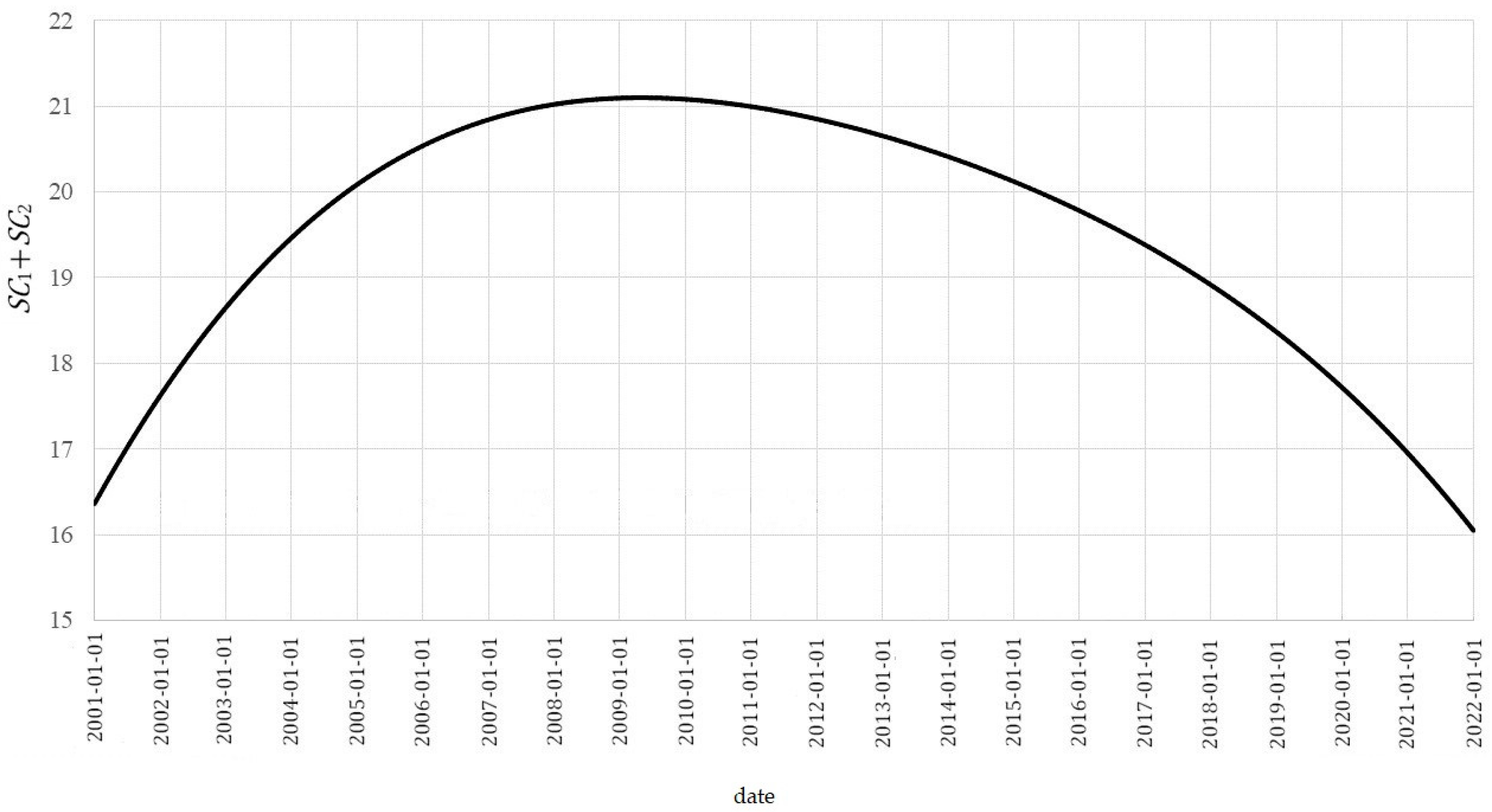
Due to the fact that 2 π b 1 = 456,366.9555 > 2 π b 2 = 402,785.3953 184,079 , the average of the first two components of the model S C 1 x + S C 2 x = a 1 sin b 1 x + c 1 + a 2 sin b 2 x + c 2 for x 1 ,   184,079 is:
j = 1 184,079 a 1 sin b 1 j + c 1 + a 2 sin b 2 j + c 2 184,079 = 19.56854515
closing to the mean of the vector Y :
j = 1 184,079 y j 184,079 = 19.67718759
and is responsible for the general trend for the data (Figure 3). It can be interpreted as a general outline of the average variability of nitrogen dioxide concentrations in the air in Polish cities over a period of 21 years. This part of the model describes the increase in the average NO2 concentration between January 2001 and May 2009 in the range from 16.3616 to 21.0975 µg/m3, followed by a decrease in average pollution to 16.0488 µg/m3 at the end of 2021.
Cyclical trends for data: for the remaining coefficients b k for k 3 , 4 , 5 , 6 , 7 , 8 , the following inequalities occur:
2 π b 4 = 11.9999 < 2 π b 6 = 23.9344 < 2 π b 5 = 24.0000 < 2 π b 8 = 24.0659 < 2 π b 7 = 167.9976 < 2 π b 3 = 8737.7286 184,079
Furthermore, the components SCk of the model (for k 3 , 4 , 5 , 6 , 7 , 8 ) can be grouped according to the type of cyclic variation in the average NO2 concentration.
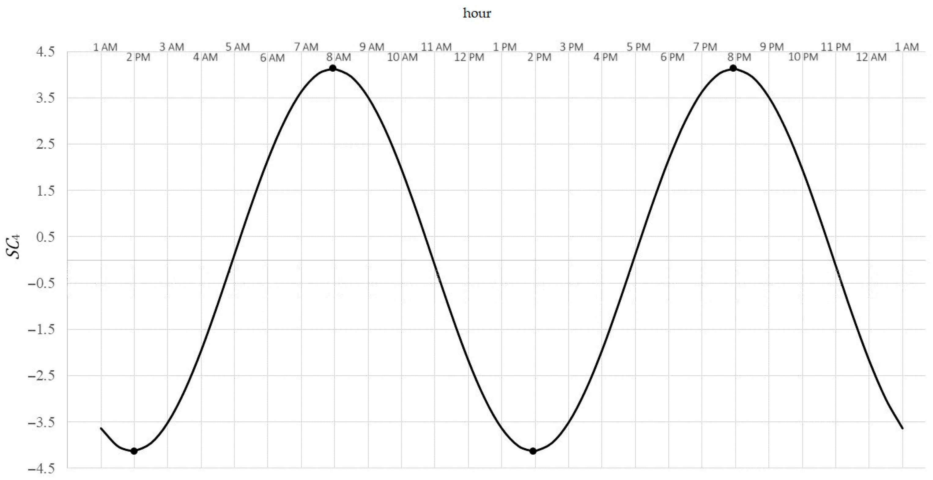
Because 2 π b 4 12 , then SC4 describes 12-h variability (day-night). In this range, the minimum SC4 is achieved for π 2 c 4 / b 4 1.9427 (that is, around 2 a.m. and 2 p.m.) and is equal 1 a 4 = 4.1294 , by this much less than the 12-h average. Maximum S C 4 achieved for π 2 c 4 / b 4 7.9427 (that is, around 8 a.m. and 8 p.m.) is equal a 4 = 4.1294 , by this much more than the 12-h average. The difference a 4 a 4 = 2 a 4 8.2588 is the amplitude of average changes during the day/night.
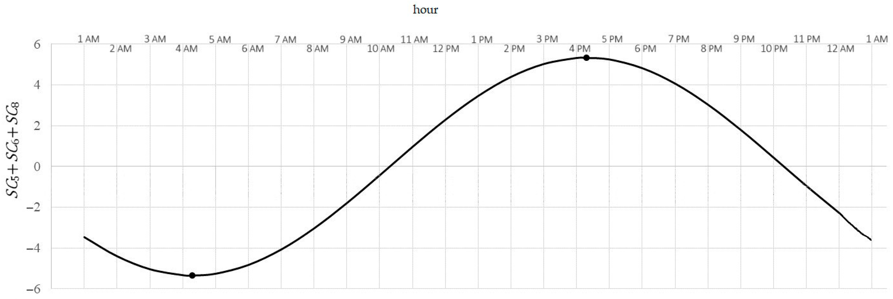
Because 2 π b 6 24 , 2 π b 5 24 i 2 π b 8 24 , therefore S C 5 + S C 6 + S C 8 describes 24-h variability (daily variability). In this range, the minimum S C 5 + S C 6 + S C 8 is achieved for x 4.305 (that is, after 4 a.m.) and is equal 5.3488 , by this much less than the 24-h average. Maximum S C 5 + S C 6 + S C 8 is achieved for x 16.3086 (after 4 o’clock p.m.) and is equal 5.3395 , by this much more than the 24-h average. The difference 5.3395 5.3488 10.6883 is the amplitude of average changes during a day.
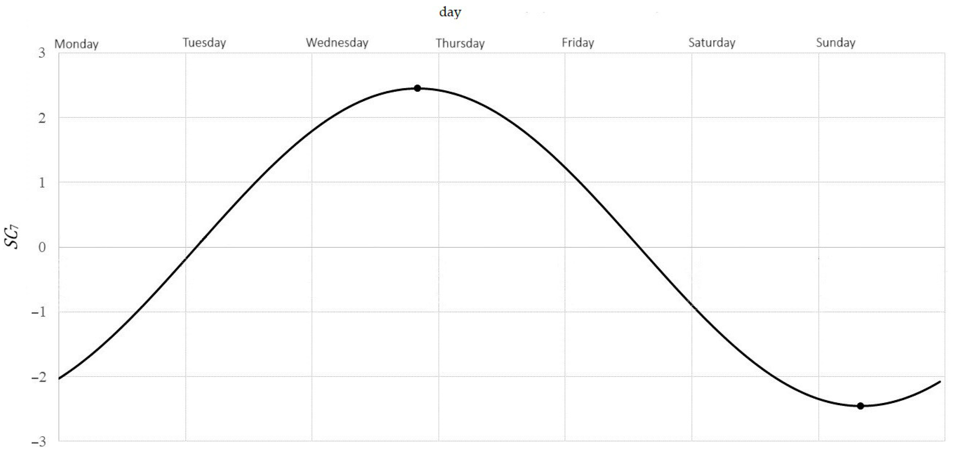
Because 2 π b 7 = 167.9976 168 = 24 7 , S C 7 describes weekly variability. In this range, the S C 7 is achieved for 3 π 2 c 7 / b 7 152.0094 (that is around 8 a.m. on Sunday morning) and is equal 1 a 7 = 2.4527 , by this much less than the weekly average. Maximum S C 7 is achieved for π 2 c 7 / b 7 68.0105 (so around 8 p.m. on Wednesday) and is equal a 7 = 2.4527 , by this much more than the weekly average. The difference a 7 a 7 4.9055 is the amplitude of average changes during a week.
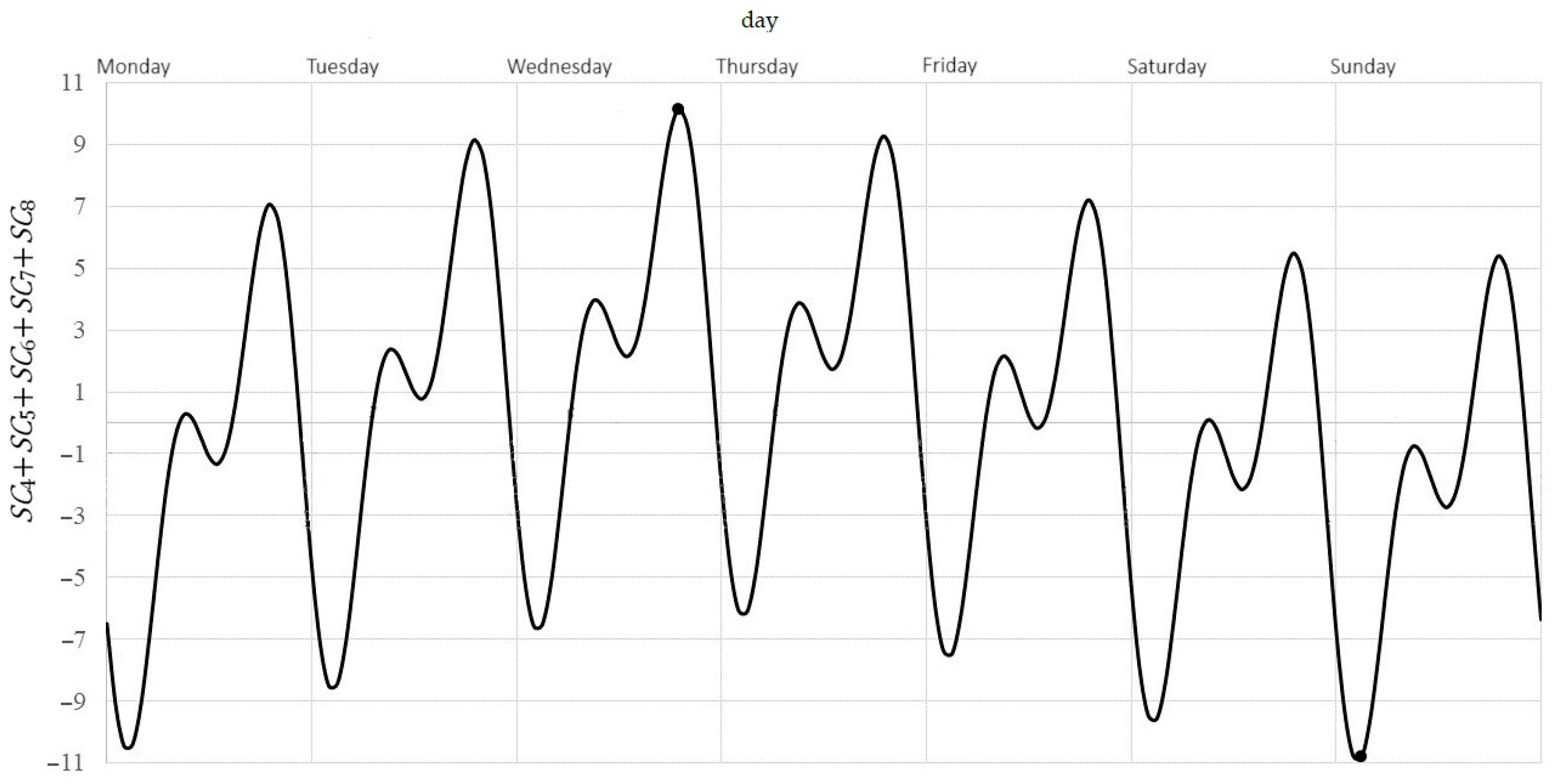
The function S C 4 + S C 5 + S C 6 + S C 7 + S C 8 can be treated as a model of the total weekly cyclical variability of NO2 concentration. This variability reaches its maximum value of 10.14 above the weekly average on Wednesday at around 7 p.m. and its minimum value −10.81 below the weekly average on Sunday at around 3 a.m. The amplitude of the total weekly cyclical changes is approximately 20.95.
Because 2 π b 3 = 8737.7286 8760 = 24 365 , S C 3 describes the annual variability. In this range minimum S C 3 is achieved for 3 π 2 c 3 / b 3 4877.22 (that is, in the third decade of July) and equals 1 a 3 = 4.5528 , by this much less than the annual average. Maximum S C 3 is achieved for π 2 c 3 / b 3 508.359 (that is, in the third decade of January) and equals a 3 = 4.5528 , by this much more than the annual average. The difference a 3 a 3 9.1056 is the amplitude of average changes during a year.
It is necessary to emphasize that the model components cannot be interpreted independently outside the context of the full model, as each component contributes uniquely and interacts with others. Each component introduces variation for every time step (hour ranging from 1 to 184,079), but in a manner that is unique to each instance and interacts with the other components within the model.
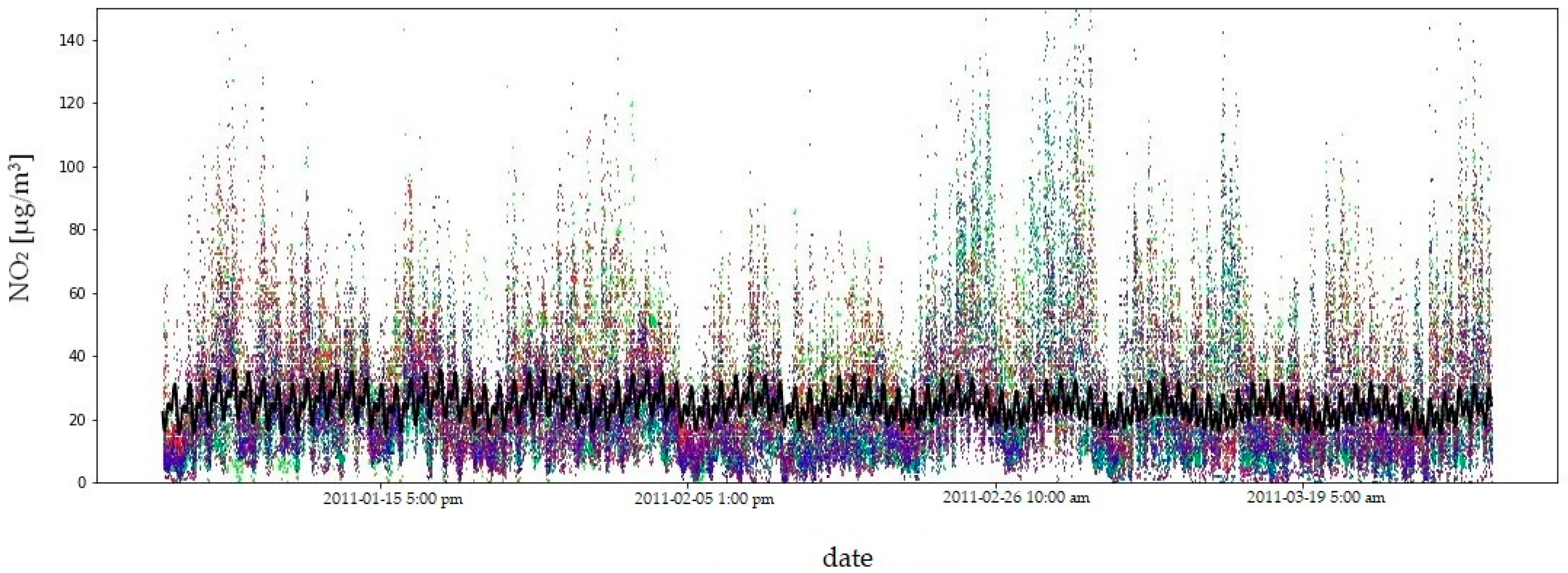
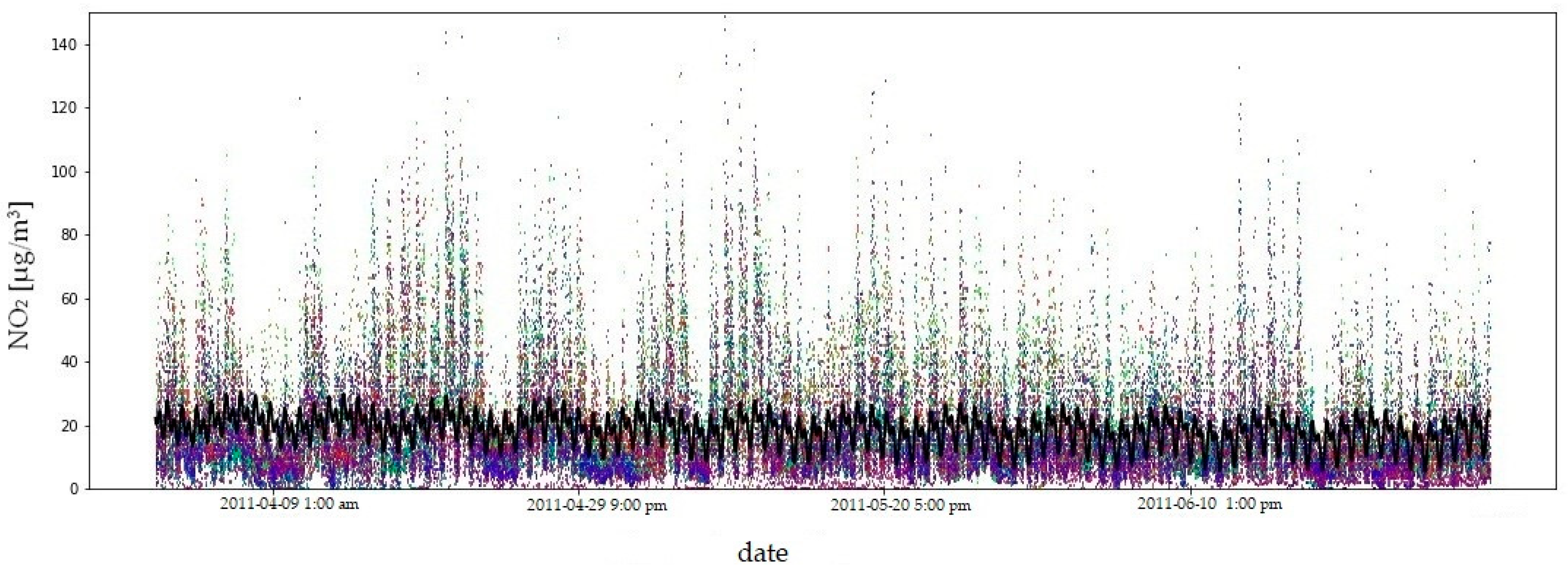
Due to the amount of data and the length of the measurement period, the fit of the model to the empirical data is illustrated using the example of four consecutive quarters of 2011 (Figure 9, Figure 10, Figure 11 and Figure 12). In order to compare the NO2 concentration variability, the value axis range was limited to 150   [ μ g / m 3 ] .

4. Discussion

In this article, we have proposed a new model consisting of the sum of sines and presented it in an explicit form. The model represents the course of NO2 concentrations in the years 2001–2021 as an averaged picture of a ‘typical city’ in Poland. The relatively low coefficient of determination partly results from the very large dataset and the uneven availability of measurements—in some hours readings may come from only a few stations, which limits averaging and affects the R2 value. In our view, it is not possible to construct a model with a small number of parameters that would achieve a high level of fit; such a model would have to be very complex and therefore less transparent and of limited practical use. Our model allowed us to identify a period of increasing NO2 concentrations until May 2009, in contrast to the situation in Western Europe (long-term trends). Furthermore, on an annual basis, it indicated the third decade of July as the period with the lowest concentrations, which is probably influenced by the reduction in traffic intensity associated with students leaving cities. In contrast, the period with the highest NO2 concentrations was in the third decade of January. Using the model, we determined the hours with the highest NO2 content in the air (8 a.m. and 8 p.m.). This model is superior in terms of the R2 coefficient of determination than the previous one based on time series [53]. Both models analysed changes in NO2 over time, but in this study we had a very large data set at our disposal. The main advantage of our model is that it does not require additional predictors; it is only a function of time.
The study contributes to existing knowledge by introducing a new model that has provided valuable information on identifying periods with the highest NO2 concentrations and can thus be used to warn the population, which is of considerable importance for children, the elderly and patients with lung diseases. In the future, it may enable decisions to be made on preventive measures such as traffic restrictions and the creation of maps of NO2 exposure risk, which is important when locating new schools or hospitals.
The proposed model is promising, and may encourage researchers to apply it in other areas and verify its usefulness.
In future work, we intend to focus on extending the analysis period to include subsequent years, especially in the context of changes to the latest WHO guidelines from 2021 [47] and the introduction of government and local programmes in Poland aimed at reducing pollutant emissions.

Author Contributions

Conceptualization, methodology, validation, formal analysis, investigation, data curation, writing—original draft preparation, visualization and final version of the manuscript, S.I., D.D. and M.S. All authors have read and agreed to the published version of the manuscript.

Funding

This research received no external funding.

Institutional Review Board Statement

Not applicable.

Informed Consent Statement

Not applicable.

Data Availability Statement

The datasets analyzed in the current study are publicly available on the following website: https://powietrze.gios.gov.pl/pjp/archives (accessed on 4 October 2023).

Conflicts of Interest

The authors declare no conflicts of interest.

Appendix A

Figure A1. Yearly NO2 concentrations measured at stations from S1 to S24. The green line of each box represents the median; the top and bottom edges of the box represent the 25th and 75th percentiles, respectively; the whiskers indicate the range of observations that are not considered outliers; blue dots represent the outliers, and the red dots represent the averages. Values on the y-axis are limited to 300   [ μ g / m 3 ] for clarity.
Sustainability 17 09456 g0a1
Figure A2. Yearly NO2 concentrations measured at stations from S25 to S47. The green line of each box represents the median; the top and bottom edges of the box represent the 25th and 75th percentiles, respectively; the whiskers indicate the range of observations that are not considered outliers; blue dots represent the outliers, and the red dots represent the averages. Values on the y-axis are limited to 300   [ μ g / m 3 ] for clarity.
Sustainability 17 09456 g0a2

References

  1. Bourdrel, T.; Bind, M.-A.; Bejot, Y.; Morel, O.; Argacha, J.-F. Cardiovascular effects of air pollution. Arch. Cardiovasc. Dis. 2017, 110, 634–642. [Google Scholar] [CrossRef] [PubMed]
  2. Goshua, A.; Akdis, C.A.; Nadeau, K.C. World Health Organization global air quality guideline recommendations: Executive summary. Allergy 2022, 77, 1955–1960. [Google Scholar] [CrossRef]
  3. Guarnieri, M.; Balmes, J.R. Outdoor air pollution and asthma. Lancet 2014, 383, 1581–1592. [Google Scholar] [CrossRef]
  4. Jiang, X.-Q.; Mei, X.-D.; Feng, D. Air pollution and chronic airway diseases: What should people know and do? J. Thorac. Dis. 2016, 8, E31–E40. [Google Scholar]
  5. Manisalidis, I.; Stavropoulou, E.; Stavropoulos, A.; Bezirtzoglou, E. Environmental and health impacts of air pollution: A review. Front. Public Health 2020, 8, 505570. [Google Scholar] [CrossRef]
  6. Mo, Z.; Fu, Q.; Lyu, D.; Zhang, L.; Qin, Z.; Tang, Q.; Yin, H.; Xu, P.; Wu, L.; Wang, X.; et al. Impacts of air pollution on dry eye disease among residents in Hangzhou, China: A case-crossover study. Environ. Pollut. 2019, 246, 183–189. [Google Scholar] [CrossRef] [PubMed]
  7. Gawełko, J.; Cierpiał-Wolan, M.; Bwanakare, S.; Czarnota, M. Association between Air Pollution and Squamous Cell Lung Cancer in South-Eastern Poland. Int. J. Environ. Res. Public Health 2022, 19, 11598. [Google Scholar] [CrossRef] [PubMed]
  8. Emberson, L.D.; Pleijel, H.; Ainsworth, E.A.; den Berg, M.; Ren, W.; Osborne, S.; Mills, G.; Pandey, D.; Dentener, F.; Büker, P.; et al. Ozone effects on crops and consideration in crop models. Eur. J. Agron. 2018, 100, 19–34. [Google Scholar] [CrossRef]
  9. Saxena, V. Water Quality, Air Pollution, and Climate Change: Investigating the Environmental Impacts of Industrialization and Urbanization. Water Air Soil Pollut. 2025, 236, 73. [Google Scholar] [CrossRef]
  10. Treder, M. Smog—A threat to health safety in Poland. Rocz. Bezpieczeństwa Międzynarodowego 2017, 11, 190–204. [Google Scholar]
  11. Lasne, J.; Lostier, A.; Salameh, T.; Athanasopoulou, E.; Karagiannis, D.; Kakouri, A.; Vassaux, S.; Lesueur, D.; Romanias, M.N. NOx emissions by real-world fresh and old asphalt mixtures: Impact of temperaturę, relative humidity, and UV-irradiation. Urban Clim. 2023, 49, 101457. [Google Scholar] [CrossRef]
  12. United Nations, Department of Economic and Social Affairs, Population Division. World Urbanization Prospects: The 2018 Revision. Available online: https://www.un.org/development/desa/pd/content/publications (accessed on 12 August 2021).
  13. The Ella Roberta Fundation. Available online: https://www.ellaroberta.org/about-ella (accessed on 6 October 2024).
  14. Health Impacts of Air Pollution in Europe. 2022. Available online: https://www.eea.europa.eu/publications/air-quality-in-europe-2022/health-impacts-of-air-pollution (accessed on 25 November 2023).
  15. Pope, C.A.; Dockery, D.W. Health Effects of Fine Particulate Air Pollution: Lines that Connect. J. Air Waste Manag. Assoc. 2006, 56, 709–742. [Google Scholar] [CrossRef]
  16. Kampa, M.; Castanas, E. Human health effects of air pollution. Environ. Pollut. 2008, 151, 362–367. [Google Scholar] [CrossRef]
  17. Brook, R.D.; Rajagopalan, S.; Brook, J.R.; Bhatnagar, A.; Diez-Roux, A.V.; Holguin, F.; Hong, Y.; Luepker, R.V.; Mittleman, M.A.; Peters, A.; et al. Particulate matter air pollution and cardiovascular disease an update to the scientific statement from the American Heart Association. Circulation 2010, 121, 2331–2378. [Google Scholar] [CrossRef]
  18. Künzli, N.; Perez, L.; Rapp, R. Air Quality and Health; European Respiratory Society: Lausanne, Switzerland, 2010; Available online: https://www.ersnet.org/wp-content/uploads/2021/03/Air-Quality-and-Health-2010.pdf (accessed on 17 December 2024).
  19. Kelly, F.J.; Fussell, J.C. Air pollution and airway disease. Clin. Exp. Allergy 2011, 41, 1059–1071. [Google Scholar] [CrossRef] [PubMed]
  20. Genc, S.; Zadeoglulari, Z.; Fuss, S.H.; Genc, K. The adverse effects of air pollution on the nervous system. J. Toxicol. 2012, 2012, 782462. [Google Scholar] [CrossRef]
  21. Ding, L.; Zhu, D.; Peng, D. Meta-analysis of the relationship between particular matter (PM(10) and PM(2.5)) and asthma hospital admissions in children. Chin. J. Pediatr. 2015, 53, 129–135. [Google Scholar]
  22. Yamazaki, S.; Shima, M.; Yoda, Y.; Oka, K.; Kurosaka, F.; Shimizu, S. Exposure to air pollution and meteorological factors associated with children’s primary care visit at night due to asthma attack: Case-crossover design for 3-tear pooled patients. BMJ Open. 2015, 5, e005736. [Google Scholar] [CrossRef]
  23. Clifford, A.; Lang, L.; Chen, R.; Anstey, K.J.; Seaton, A. Exposure to air pollution and cognitive functioning across the life course—A systematic literature review. Environ. Res. 2016, 147, 383–398. [Google Scholar] [CrossRef] [PubMed]
  24. Krzyżanowski, M. Wpływ zanieczyszczenia powietrza pyłami na układ krążenia i oddychania. Lek. Wojsk. 2016, 1, 17–22. [Google Scholar]
  25. Wojdat, M.; Stańczyk, A.; Gielerak, G. Zanieczyszczenia powietrza a choroby układu sercowo-naczyniowego—Niedoceniany problem. Lek. Wojsk. 2016, 1, 10–16. [Google Scholar]
  26. Compa, M.F.; Baumbach, C.; Kaczmarek-Majer, K.; Buczyłowska, D.; Gradys, G.; Skotak, K.; Degórska, A.; Bratkowski, J.; Wierzba-Łukaszyk, M.; Mysak, Y.; et al. Air Pollution and Attention in Polish Schoolchildren with and without ADHD. Sci. Total Environ. 2023, 892, 164759. [Google Scholar] [CrossRef]
  27. Thurston, G.D.; Kipen, H.; Annesi-Maesano, I.; Balmes, J.; Brook, R.D.; Cromar, K.; De Matteis, S.; Forastiere, F.; Forsberg, B.; Frampton, M.W.; et al. A joint ERA/ATS policy statement: What constitutes an adverse health effect of air pollution? An analytical framework. Eur. Respir. J. 2017, 49, 1600419. [Google Scholar] [CrossRef]
  28. First, M.W. HEPA filters. J. Am. Biol. Saf. Assoc. 1998, 3, 33–42. [Google Scholar] [CrossRef]
  29. Liao, J.; Ye, W.; Pillarisetti, A.; Clasen, T.F. Modeling the Impact of Indoor Air Folter on Air Pollution Exposure Reduction and Associated Mortality in Urban Household. Int. J. Environ. Res. Public Health 2019, 16, 1391. [Google Scholar] [CrossRef] [PubMed]
  30. Dreisbach, R.H.; Robertson, W. Vademecum Zatruć: Zapobieganie, Rozpoznawanie I Postępowanie; PZWL: Warszawa, Poland, 1995. [Google Scholar]
  31. Eum, K.; Honda, T.J.; Wang, B.; Kazemiparkouhi, F.; Manjourides, J.; Pun, V.C.; Suh, H. Long-term nitrogen dioxide exposure and cause-specific mortality in the U.S. Medicare Population. Environ. Res. 2022, 207, 112154. [Google Scholar] [CrossRef]
  32. Krzyżanowski, M. Wpływ Zanieczyszczenia Powietrza Atmosferycznego Dwutlenkiem Azotu na Zdrowie. 2023. Available online: https://healpolska.pl/wp-content/uploads/2023/06/NO2_a_zdrowie20230629_PL.pdf (accessed on 12 June 2023).
  33. Bărbulescu, A.; Hosen, K. Cement Industry Pollution and Its Impact on the Environment and Population Health: A Review. Toxics 2025, 13, 587. [Google Scholar] [CrossRef]
  34. Křůmal, K.; Mikuška, P.; Horák, J.; Hopan, F.; Kuboňová, L. Influence of boiler output and type on gaseous and particulate emissions from the combustion of coal for residential heating. Chemosphere 2021, 278, 130402. [Google Scholar] [CrossRef] [PubMed]
  35. Wang, Y.; Yao, Z.; Zheng, X.; Subramaniam, L.; Butterbach-Bahl, K. A synthesis of nitric emissions across global fertilized croplands from crop-specific emission factors. Glob. Change Biol. 2022, 28, 4395–4408. [Google Scholar] [CrossRef]
  36. Air Quality in Europe 2022. Sources and Emissions of Air Pollutants in Europe. Available online: https://www.eea.europa.eu/publications/air-quality-in-europe-2022/sources-and-emissions-of-air (accessed on 17 September 2023).
  37. A Technical Summary of Euro 6/VI Vehicle Emission Standards. Available online: https://theicct.org/sites/default/files/publications/ICCT_Euro6-VI_briefing_jun2016.pdf (accessed on 11 January 2024).
  38. Average Age of the EU Vehicle Fleet, by Country—ACEA—European Automobile Manufacturers’ Association. Available online: https://www.acea.auto/figure/average-age-of-eu-vehicle-fleet-by-country/ (accessed on 29 September 2024).
  39. Available online: https://trueinitiative.org/insights/new-true-analysis-shows-imported-used-light-duty-vehicles-in-warsaw-emit-two-to-three-times-as-much-pollution-as-domestic-vehicles?tag=Brussels/ (accessed on 25 May 2024).
  40. Bernard, Y.; Tietge, U.; Pniewska, I. Remote Sensing of Motor Vehicle Emissions in Krakow. 2020. Available online: https://theicct.org/wp-content/uploads/2021/06/Remote-sensing-Krakow-sept2020-1.pdf (accessed on 25 May 2024).
  41. Centralna Ewidencja Pojazdów i Kierowców. Available online: https://www.gov.pl/web/cepik (accessed on 3 March 2024).
  42. Bank Danych Lokalnych. Available online: https://bdl.stat.gov.pl/bdl/dane/podgrup/temat (accessed on 11 March 2024).
  43. Regulation (EU) 2023/851 of the European Parliament and of the Council of 19 April 2023 amending Regulation (EU) 2019/631 as regards strengthening the CO2 emission performance standards for new passenger cars and new light commercial vehicles in line with the Union’s increased climate ambition (OJ L 110, 25.4.2023, pp. 5–20). Available online: https://eur-lex.europa.eu/legal-content/EN/TXT/?uri=CELEX%3A32023R0851 (accessed on 11 March 2024).
  44. Directive 2008/50/EC of the European Parliament and of the Council of 21 May 2008 on Ambient Air Quality and Cleaner Air for Europe. Available online: https://www.eumonitor.eu/9353000/1/j9vvik7m1c3gyxp/vhvvygrp44xc (accessed on 3 March 2024).
  45. Ustawa z Dnia 27 Kwietnia 2001, r. Prawo Ochrony Środowiska. Available online: https://isap.sejm.gov.pl/isap.nsf/DocDetails.xsp?id=wdu20010620627 (accessed on 4 December 2023).
  46. Rozporządzenie Ministra Środowiska z Dnia 24 Sierpnia 2012 r. w Sprawie Poziomów Niektórych Substancji w Powietrzu. Available online: https://isap.sejm.gov.pl/isap.nsf/DocDetails.xsp?id=WDU20120001031 (accessed on 4 December 2023).
  47. Available online: https://www.who.int/news-room/feature-stories/detail/what-are-the-who-air-quality-guidelines (accessed on 4 December 2023).
  48. Wielgosiński, G.; Czerwińska, J.; Niemiecińska, O.; Cichowicz, R. Smog episodes in the Lodz agglomeration in the years 2014–17. In Proceedings of the E3S Web of Conferences, Zakopane, Poland, 18–21 October 2018; Volume 28, p. 01039. [Google Scholar] [CrossRef]
  49. Sówka, I.; Chlebowska-Styś, A.; Pachurka, Ł.; Rogula-Kozłowska, W.; Mathews, B. Analysis of particular matter concentration variability and origin in selected urban areas in Poland. Sustainability 2019, 11, 5735. [Google Scholar] [CrossRef]
  50. GIOŚ. Available online: https://powietrze.gios.gov.pl/pjp/maps/measuringstation (accessed on 4 October 2023).
  51. Standard PN-EN 14211:2013-02; Atmospheric Air—Standard Method for Measuring the Concentration of Nitrogen Dioxide and Nitrogen Oxide Using Chemiluminescence. Polski Komitet Normalizacyjny: Warszawa, Poland, 2013.
  52. GIOŚ. Available online: https://powietrze.gios.gov.pl/pjp/archives (accessed on 4 October 2023).
  53. Ignaciuk, S.; Wawrzosek, J.; Zarajczyk, J.; Choszcz, D. Periodisity of changes in nitrogen oxides concentrations in the urban environment, Part 2. Nitrogen dioxide concentration. Przemysł Chem. 2019, 98, 1927–1929. [Google Scholar]
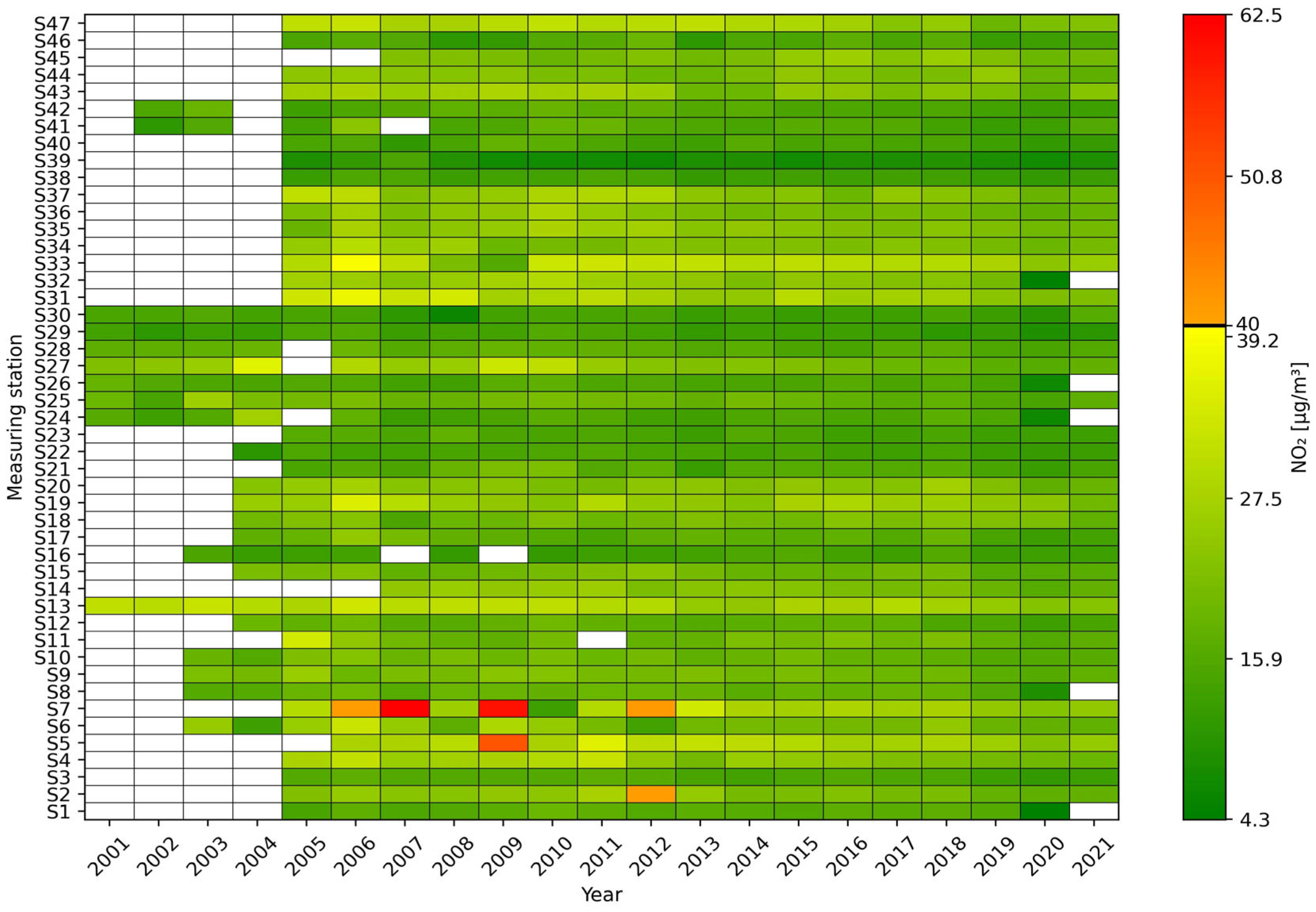
Figure 1. Annual mean concentrations of NO2 [µg/m3] at monitoring stations S1–S47 in the years 2001–2021 presented as a heat map. The value of 40 µg/m3 is highlighted on the color scale, which the WHO recommended as the maximum permissible annual mean concentration until 2021.
Sustainability 17 09456 g001
Figure 2. Interpretation of model components of NO2 concentration.
Sustainability 17 09456 g002
Figure 3. General trend.
Sustainability 17 09456 g003
Figure 4. Typical pattern of cyclic 12-h variability of NO2 concentration.
Sustainability 17 09456 g004
Figure 5. Typical pattern of cyclic 24-h variability of NO2 concentration.
Sustainability 17 09456 g005
Figure 6. Typical pattern of cyclic weekly variability of NO2 concentration.
Sustainability 17 09456 g006
Figure 7. Typical pattern of total weekly variability of NO2 concentration.
Sustainability 17 09456 g007
Figure 8. Typical pattern of cyclic annual variability of NO2 concentration.
Sustainability 17 09456 g008
Figure 9. NO2 concentrations in the first quarter of 2011: model fit shown as a black line, observed data in colour. The coefficient of determination ( R 2 = 0.3366 ) quantifies the goodness of fit of the model to the observed data.
Sustainability 17 09456 g009
Figure 10. NO2 concentrations in the second quarter of 2011: model fit shown as a black line, observed data in colour. The coefficient of determination ( R 2 = 0.3366 ) quantifies the goodness of fit of the model to the observed data.
Sustainability 17 09456 g010
Figure 11. NO2 concentrations in the third quarter of 2011: model fit shown as a black line, observed data in colour. The coefficient of determination ( R 2 = 0.3366 ) quantifies the goodness of fit of the model to the observed data.
Sustainability 17 09456 g011
Figure 12. NO2 concentrations in the fourth quarter of 2011: model fit shown as a black line, observed data in colour. The coefficient of determination ( R 2 = 0.3366 ) quantifies the goodness of fit of the model to the observed data.
Sustainability 17 09456 g012
Table 1. Geographical coordinates of measuring stations S1–S47.
SymbolInternationale
Code
City/TownWGS84 φ NWGS84 λ E
S1PL0187ADzierżoniów50.73281716.648050
S2PL0190ALegnica51.20450316.180513
S3PL0192AWałbrzych50.76872916.269677
S4PL0194AWrocław51.12937817.029250
S5PL0252ABydgoszcz53.12177417.987883
S6PL0064ABydgoszcz53.13408817.995712
S7PL0205AWłocławek52.65846719.059314
S8PL0096AŁódź51.75805019.529786
S9PL0104APabianice51.66798119.368683
S10PL0115AZgierz51.85669219.421231
S11PL0209AGorzów Wielkopolski52.73821415.228667
S12PL0213AZielona Góra51.93978315.518861
S13PL0039AKraków50.06930820.053492
S14PL0273ASkawina49.97104719.830422
S15PL0126AZakopane49.29356419.960083
S16PL0398APłock52.55627919.687672
S17PL0136APłock52.55093819.709791
S18PL0138ARadom51.39908421.147474
S19PL0143AWarszawa52.29086421.042458
S20PL0141AWarszawa52.16077221.033819
S21PL0218AKędzierzyn-Koźle50.34960818.236575
S22PL0148ABiałystok53.12668923.155869
S23PL0151AŁomża53.18139422.054381
S24PL0046AGdańsk54.36777818.701111
S25PL0052AGdańsk54.38027918.620274
S26PL0049AGdańsk54.32833618.557781
S27PL0045AGdańsk54.35333618.635283
S28PL0047AGdańsk54.40083318.657497
S29PL0048AGdynia54.56083618.493331
S30PL0050ASopot54.43166718.579722
S31PL0237ADąbrowa Górnicza50.32911119.231222
S32PL0238AGliwice50.27948118.655736
S33PL0008AKatowice50.26461118.975028
S34PL0239ARybnik50.11118118.516139
S35PL0240ATychy50.09990318.990236
S36PL0241AWodzisław Śląski50.00762918.455548
S37PL0242AZabrze50.31650018.772375
S38PL0295AElbląg54.16784719.410942
S39PL0312AGołdap54.30590822.307681
S40PL0175AOlsztyn53.78923320.486075
S41PL0031AKonin52.22563318.269036
S42PL0468APiła53.15440816.759572
S43PL0245APoznań52.42031916.877289
S44PL0244APoznań52.39817516.959519
S45PL0298AKoszalin54.19398616.172544
S46PL0248ASzczecin53.38097514.663347
S47PL0249ASzczecin53.43216914.553900
Disclaimer/Publisher’s Note: The statements, opinions and data contained in all publications are solely those of the individual author(s) and contributor(s) and not of MDPI and/or the editor(s). MDPI and/or the editor(s) disclaim responsibility for any injury to people or property resulting from any ideas, methods, instructions or products referred to in the content.