Research on Landscape Risks and Their Driving Mechanisms for Sustainable Development in Alpine Meadow Areas

Abstract

Landscape Ecological Risk Assessment (LERA) is the basis for stable ecological functions in alpine meadow areas and is closely related to sustainable development. The research of LERA is complex, and there are problems with its identification scale and method selection. Existing LERA studies are relatively limited in focusing on alpine meadow areas. Therefore, we explored the characteristics of landscape ecological risk (LER) and its driving mechanisms in Gannan (GN) using the Landscape Ecological Risk Index (LERI) and GeoDetector at the grid scale based on the 2000–2020 CNLUCC data and other ancillary data. Results demonstrated the following: (1) From 2000 to 2020, grasslands and woodlands were the major landscape types in GN. Landscape changes mainly occurred between grasslands and woodlands. (2) During the time of the research, the overall environmental patch fragmentation and complexity of the study area increased. (3) LER in GN is dominated by medium-low and medium risk, while the overall trend of LER is decreasing. (4) The effect of natural factors on the evolution of the LER pattern in GN is greater than the effect of socio-economic factors. The elevation factor has the greatest impact among all factors. Additionally, the interaction of the factors on the evolution of LER was enhanced. Consequently, scientific artificial restoration works and maintaining a reasonable area of croplands are crucial for LER control. This study offers an important reference for fine-scale LERA research and provides a scientific basis for ecological management and sustainable development in the alpine meadow regions.

1. Introduction

As the effects of climate change and human activities are increasing, ecological risks have become a major challenge for global ecosystems [1]. The Environment and Development Report 2022 stated that overexploited landscape patterns pose serious ecological risks [2]. LERA, as a concrete manifestation of ecological risk research, effectively supports regional ecological management and decision-making. Alpine meadow regions are one of the world’s important ecological barriers and water conservation areas [3]. However, studies indicated that climate change and human activities pose severe threats to biodiversity and water retention functions in these regions [4]. This is particularly evident across the Qinghai–Tibet Plateau. Landscape ecological risk (LER) issues on the Qinghai–Tibet Plateau have garnered significant global scientific concern [5]. Therefore, LERA research is of great significance to the sustainable development of alpine meadow regions.

Under the context of climate change and economic development, alpine meadow regions must reconcile developmental demands at the regional scale. Complex risk sources affect ecological security by altering landscape patterns. This necessitates an analysis of the spatiotemporal dynamics and driving forces of regional ecological risk. LERA serves as a mainstream methodology for the integrated representation and spatialization of multi-source risks. It is characterized by its emphasis on the spatiotemporal heterogeneity and scale effects of risk [6,7]. At present, the approaches commonly used for LERA include the “source-sink” landscape theory [8], the Relative Risk Model [9], and the Landscape Ecological Risk Index (LERI) [10]. The “source-sink” landscape theory and the Relative Risk Model help to understand the interactions between regional LER and regions [11]. However, the “source-sink” landscape theory is more difficult to analyze the risk situation under multiple stressors, and it is challenging to validate the robustness of the relative risk model and the accuracy of the results [12].

With the deepening of research, LERI has been proposed to determine the spatial and temporal evolution of ecological risk in landscapes. Compared with the source-sink landscape theory, LERI can more effectively assess the LER status of areas with multi-source pressure effects under long-term series. Moreover, the results are more accurate and stable as compared to relative risk models [13]. In recent years, LERI has been used in regional LERA in coastal areas [14] and watersheds [15], which indicates that LERI can be widely applied to LERA at different spatial scales. Therefore, we investigated dynamic LERA for alpine meadow regions using LERI.

Furthermore, the methodological approach to driver analysis constitutes a critical aspect influencing Landscape Ecological Risk Assessment (LERA) outcomes. Quantitatively assessing the influence of driving factors provides precise spatial decision-making support for regional ecological risk management and control. Current investigations of LER determinants predominantly employ correlation and regression models [16]. Traditional regression approaches exhibit limited capacity to analyze synergistic/antagonistic interactions among driving factors and their spatial interdependencies. In contrast, GeoDetector has been widely adopted for examining composite driving forces of LER. This method quantifies the proportional contribution of drivers to LER spatial heterogeneity through its core metric, which is the factor detector’s q-statistic. GeoDetector has the advantages of quantitatively analyzing spatial heterogeneity, efficiently handling high-dimensional data with multiple influencing factors, and effectively dealing with non-linear relationships [17,18]. Moreover, GeoDetector was employed in various domains such as environmental science [19], ecology [20], urban planning [21], and agriculture [22]. Accordingly, we used GeoDetector to investigate the driving mechanisms of LER in a typical alpine meadow region.

Alpine meadow areas are widely distributed in high latitude or alpine zones around the world and have special significance in terms of ecological stability and biodiversity [23]. China has the largest area of alpine meadows in the world, most of which are found in the Qinghai–Tibetan Plateau (QTP) [24]. GN is positioned in the northeastern part of QTP with a characteristic alpine meadow landscape with interwoven rivers, lakes, and wetlands due to its alpine plateau hilly terrain and highland climate [25]. Consequently, GN is a typical area for conducting research on alpine meadow regions. In recent years, many scholars have studied LER in the alpine meadow regions of GN. However, different studies have different focuses, such as ecological risk identification [26], landscape pattern [27], grassland vulnerability [25], and pollution impacts [5]. The previous studies provide reference and support for this study. However, studies on systemic LER and its driving factors remain scarce [28,29]. In addition, the existing LER studies in GN areas focus on district-county scale LERA and require higher spatial precision analyses. It has been demonstrated that studies based on grid scales have higher spatial resolution and more accurate risk identification than district and county scales [30]. Therefore, we conducted a representative study of LERA and its driving mechanisms in the GN alpine meadow region based on the grid scale.

To investigate the evolutionary characteristics of LER in alpine meadow regions, we conducted the LERA based on fine-grained grid scales. Initially, we analyzed landscape patterns and evolutionary trajectories in the study region using multi-temporal CNLUCC datasets. Subsequently, we integrated the LERI with GeoDetector to examine LER dynamics and identify composite driving forces. This study provides critical support for ecological conservation and sustainable development initiatives in alpine meadow ecosystems.

2. Materials and Methods

2.1. Study Area

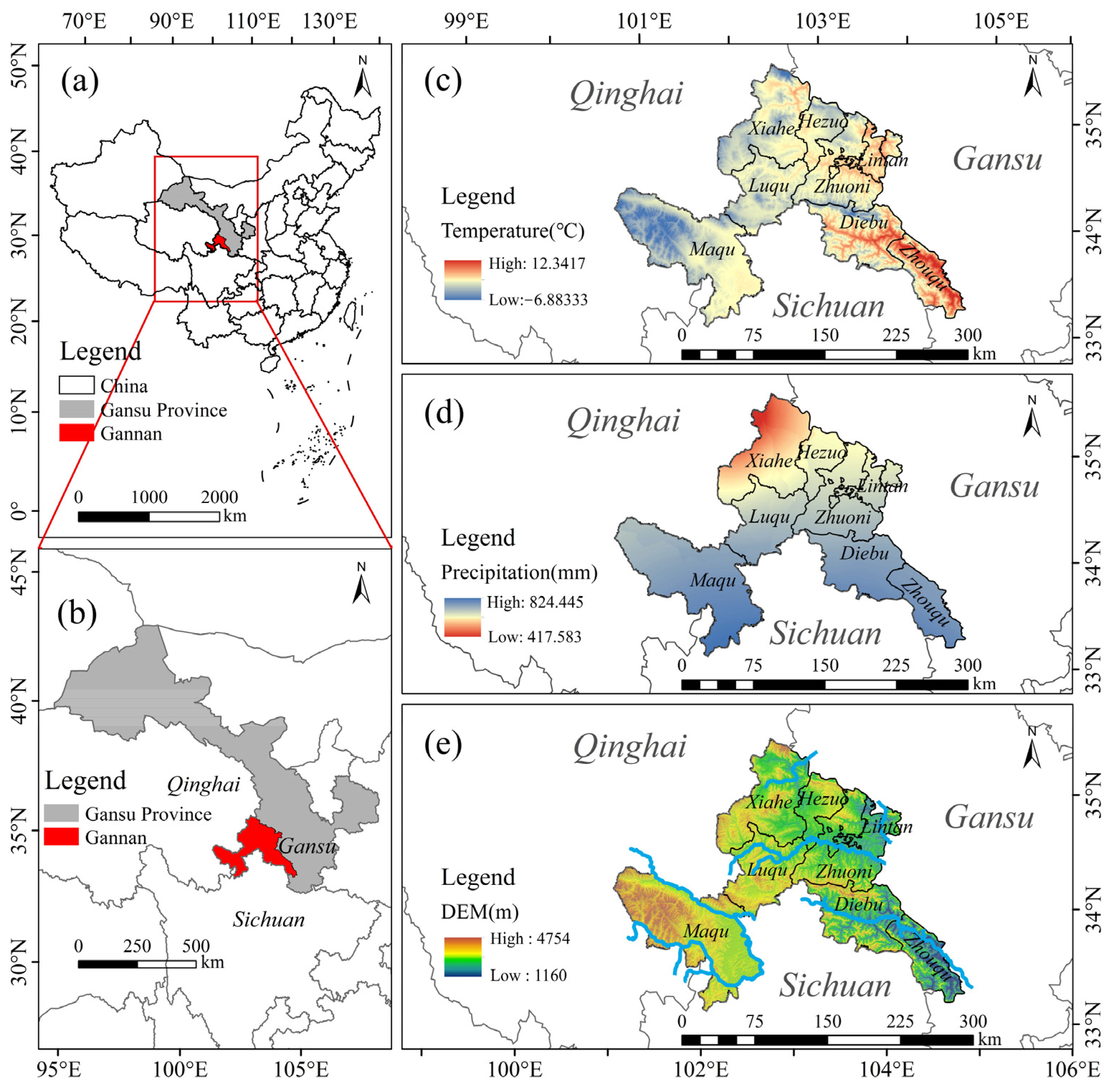
Gannan Prefecture is positioned at 33°06′30″~35°34′00″ N, 100°45′45″~104°45′30″ E (Figure 1), which is in the south of Gansu Province and the northeastern edge of QTP.

The GN includes 7 counties and 1 city, including Hezuo, Lintan, Zhuoni, Diebu, Zhouqu, Xiahe, Maqu, and Luqu, with an overall area of 3.8 × 10⁴ km² [7]. The topography is northwestern high and southeastern low, with intricate terrain [31]. The southern part of the GN consists of the Diemin Mountains, the eastern part of the GN consists of hilly areas, and the western part of the GN consists of flat grasslands. The altitude of GN is mostly 1160~4754 m, mostly developing alpine meadows, scrubs, and mountain forests [32]. The climate type of GN is continental climate. Precipitation demonstrates more in the southeast and less in the northwest. Since the 20th century, the socio-economic environment of GN has undergone remarkable changes. According to statistics, the population of GN increased from 653,500 people in 2000 to 752,200 people in 2020 [33]. The GDP of GN also increased rapidly from USD 190 million in 2000 to USD 3010 million in 2020 [34].

2.2. Data Sources and Descriptions

We used information from remote sensing data, weather measurements, and statistics. We can see where the information came from in

Table 1. Data sources used in this study.

Category	Data	Resolution	Data Resource
Remote sensing data	Land use/cover data	Raster (30 m)	Resource and Environment Data Center of the Chinese Academy of Sciences (https://www.resdc.cn/) (accessed on 29 January 2024)
	ASTER GDEM	Raster (30 m)	The geospatial data cloud website (https://www.gscloud.cn/) (accessed on 29 January 2024). This data is used to obtain elevation data.
	Slope data	Raster (30 m)
	Road data	Raster (30 m)	National Centre for Basic Geographic Information (https://www.webmap.cn) (accessed on 29 January 2024)
	Hydrological data	Raster (30 m)
Meteorological data	Annual average temperature	Raster (1 km)	National Science and Technology Basic Conditions Platform-Earth System Science Data Centre (http://www.geodata.cn) (accessed on 29 January 2024)
	Cumulative annual precipitation	Raster (1 km)
Statistical data	GDP	Raster (1 km)	Resource and Environment Data Center of the Chinese Academy of Sciences (https://www.resdc.cn/) (accessed on 29 January 2024)
	Population density	Raster (1 km)	WorldPop (https://hub.worldpop.org) (accessed on 29 January 2024)

.

Remote sensing data: (1) Land use/cover data: CNLUCC data at a 30 × 30 m scale for five periods between 2000 and 2020. The original data used in this study were derived from Landsat series satellite imagery provided by the United States. The Landsat satellite data has a revisit cycle of 16 days. Through a combination of manual visual interpretation and machine learning techniques, the data were analyzed and classified, ultimately establishing a multi-temporal land use/cover monitoring database at a 1:100,000 scale covering the entire country. Given the availability of land use data for five periods (2000, 2005, 2010, 2015, and 2020), this study selected these five time points for conducting landscape ecological risk assessment and driving force analysis. (2) Digital Elevation Model (DEM) data: Elevation data can be obtained directly. Slope data acquired through ArcGIS 10.8 processing. (3) Road and water system data: We downloaded this part of data and used ArcGIS software to calculate the distance of the road and water system from the ecological risk community.

Meteorological data: We acquired data on annual mean temperatures and cumulative annual precipitation from a spatially interpolated dataset of meteorological variables in China. This dataset is derived from daily observation records of meteorological elements collected at various stations throughout China. The annual spatial interpolation dataset is created using Anuspl 4.3 interpolation software, which calculates the annual values for each meteorological parameter.

Statistical data: We sourced GDP data from the China GDP spatial distribution dataset, which features a 1 km × 1 km spatial grid. This dataset is produced through spatial interpolation of national sub-county GDP statistics, integrated with additional economic information. The population density information is sourced from the WorldPop dataset. This data set provides high-resolution spatial data on global population distribution and includes population data from various time intervals worldwide.

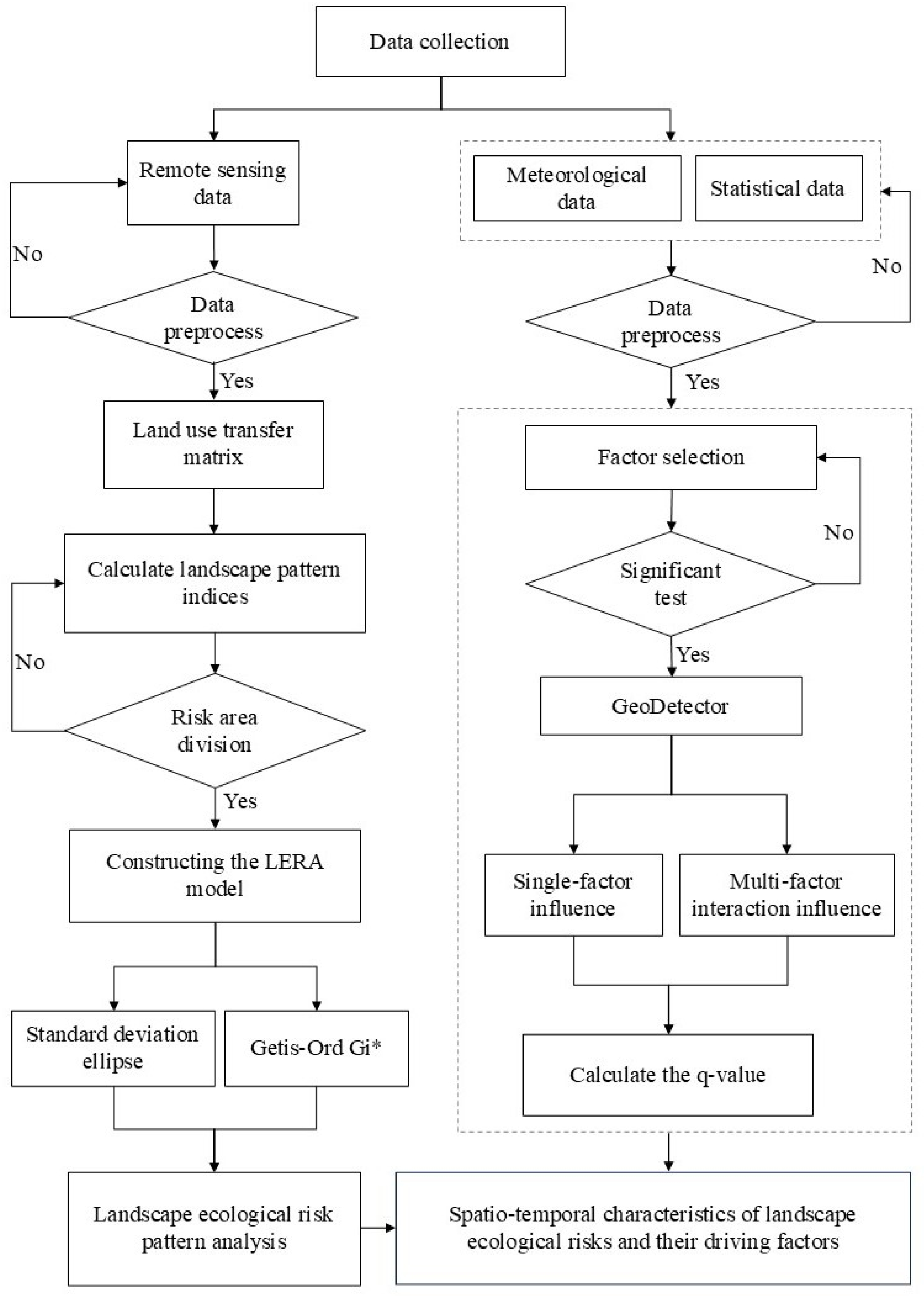
In this study, we standardized the spatial resolution of all datasets used for LERA and GeoDetector analyses to 30 m. Additionally, all geospatial data were unified to the GCS_WGS_1984 geographic coordinate system. The study area boundary was obtained from the National Platform for Common Geospatial Information Services (https://www.tianditu.gov.cn/). All research data were clipped using extracted the study area shapefile boundaries corresponding to GN. Figure 2 illustrates the methodological diagram of this study.

2.3. Research Methodology

2.3.1. Land Use Transfer Matrix

Land use transfer matrix (LUTM) is a way to study how land is used differently over time. LUTM looks at how many things are exchanged and which way they go between different groups. LUTM is often used to study how land is used in a specific area over time, including why it changes and what effect it has. It constitutes how various land types have evolved over a specific period [35].

$$S_{ij}=\left[\begin{array}{cccc}{S}_{11}& S_{12}& \dots & S_{1n}\\ S_{21}& S_{22}& \dots & S_{2n}\\ ⋮& ⋮& ⋮& ⋮\\ S_{n1}& S_{n2}& \dots & S_{nn}\end{array}\right]$$

(1)

where S_ij represents the area from type i before the transfer to type j after the transfer; n means number of types.

2.3.2. Selection and Calculation of Landscape Indexes

LPI is used to quantify the characteristics of landscape spatial layout. It reflects the composition of the landscape in GN and is also a high generalization of landscape pattern information.

To determine the scale and complexity of GN, the class level was analyzed, and four LPI were selected to capture the landscape characteristics of GN [36,37]. The specific landscape indexes are listed in

Table 2. Landscape pattern indexes selection.

Landscape Pattern Index	Formula	Ecological Implications
Patch Density (PD) [29]	$PD=NP/A$	NP defines the number of patches; A denotes the total area of patches.
Mean Patch Size (MPS) [38]	$MPS={\displaystyle \frac{{\displaystyle \sum _{\mathrm{i}=1}^N{A}_{\mathrm{i}}}}{N}}$	Ai is the area of patch i; N illustrates the total number of patches.
Landscape Shape Index (LSI) [39]	$LSI={\displaystyle \frac{4\pi \cdot A}{P^2}}$	A signifies the area of the patch; P embodies the perimeter of the patch.
Aggregation Index (AI) [40]	$AI=\left[{\displaystyle \frac{{\mathrm{g}}_{\mathrm{ii}}}{\max \to {\mathrm{g}}_{\mathrm{ii}}}}\right]\left(100\right)$	The gii reveals the number of similar adjacent patches for the corresponding landscape type.

.

2.3.3. Risk Area Division

In order to spatially present the LERI, we used grids for systematic sampling of GN. For analyses to be precise and effective, the dimensions of risk plots should range from two to five times the average patch. All plots ≥ 0.5 times the size of the standard sample area are given a separate sample area number, otherwise they are automatically merged into the nearest adjacent sample area [41]. In addition, we combine the realities of GN. Therefore, the risk area is divided into 12 km × 12 km risk area sampling grid. The total of 336 risk areas was divided as samples for ecological risk collection. Using this model, we computed the LERI for each assessment unit and used it as a sample for the analysis process that followed.

2.3.4. Construction of LERI Model

Landscape loss degree means how much the natural features of different landscapes are lost when they are disturbed by nature or people [42,43]. Different indexes are superimposed, and the landscape loss index is computed using the following formula (

Table 3. Assignment of vulnerability index.

Landscape Type	Level	Vi
cropland	4	0.19
woodland	2	0.10
grassland	3	0.14
water	5	0.24
urban land	1	0.05
unused land	6	0.29

):

$$R_i=E_i\times V_i$$

(2)

where R_i represents the landscape loss index, E_i means the landscape disturbance index, and V_i is the vulnerability index. We assigned V_i for different landscape types according to vulnerability levels based on previous research and the characteristics of the study area [44]. First, the vulnerability grading for different landscape types was as follows: 6 for unused land, 5 for water, 4 for cropland, 3 for grassland, 2 for woodland, and 1 for urban land. After normalization, the weight of the vulnerability index V_i of each landscape type is obtained (Table 3).

Further calculation of landscape loss index. On this basis, the LERI [45] is as follows:

$$LER{I}_i={\displaystyle {\sum }_{i=1}^n\frac{A_{ki}}{A_k}}\times R_i$$

(3)

where R_i is the landscape loss index, A_ki denotes the area of the type i in a risk cell, A_k illustrates the total area of a risky cell, and n is the landscape type. LERI_i is the LERI of risk community i. The higher the value, the higher the degree of ecological risk; on the contrary, the lower the degree of LER (

Table 4. LER index and its significance title of table.

Index Name	Definition	Formula	Parameter Meaning
Landscape Fragmentation Index [46]	Complexity of spatial distribution of landscape types after encountering external disturbances.	$C_{\mathrm{i}}={\displaystyle \frac{{\mathrm{n}}_i}{A_i}}$	Ai represents the area of landscape type i, while ni exhibits the number of patches.
Landscape Separation Index [47]	Complexity of the shape of landscape types at a given scale.	$N_i={\displaystyle \frac{A}{2A_i}}\sqrt{{\displaystyle \frac{n_i}{A_i}}}$	A is the sum of the areas of the studied landscapes, and Ai and ni are represented in the same way as in the previous equation.
Landscape Dimension Index [10]	Level of patch heterogeneity in a certain landscape.	$F_{\mathrm{i}}=2\ln \left({\displaystyle \frac{p_i}{4}}\right)/\ln A_i$	Pi encapsulates the perimeter of landscape type i.
Landscape Intrusiveness Index [48]	Extent of anthropogenic disturbance of the landscape.	$E_i=a{C}_i+b{N}_i+c{F}_i$	The values for the index weights are a, b, and c. Weights of 0.5, 0.3, and 0.2 were given out, in that order.

).

We used Fragstats 4.2 to calculate the size, number, and type of areas in different risk zones in GN. We then calculated the LERI based on the above indices. It is helpful to look at how ecological risk is spread out by giving it a grade. Utilizing ArcGIS 10.8.1 (License Type: Advanced), we divided the LERI into five distinct grades.

2.3.5. Evolution Pattern Analysis

The standard deviation ellipse (SDE) is used to measure geographical features. The SDE method helps us understand how to spread out and in which direction geographical elements are located on a map. It reveals the average location, direction of spread, and degree of scattering of elements. Owing to these capabilities, it is widely used to describe the evolution patterns of geographical events in areas such as landscape, economic patterns, terrain distribution, tourism, and religion [49].

To make the SDE, we used the middle point of the ellipse, the angle it is turned, and the length of the longer and the shorter sides. The center of the SDE is determined by the standing and weight of geographical events. The angle of rotation is the angle of clockwise rotation using the long axis as a reference [50]. In terms of spatial statistics, the standard deviation is calculated to obtain the long and short half axes. We utilize the SDE and its centroid shift to examine the variations in LER areas across different levels, and further intuitively analyze the pattern evolution of LER [51].

We also conducted an analysis of spatial clustering in LER using the Hotspot analysis tool of the ArcGIS 10.8.1 (License Type: Advanced). Hotspot calculates a Getis-Ord Gi* statistic for each feature in the dataset, enabling precise localization of the spatial extent and positions of both hot spots and cold spots on the map. The calculation was performed using the following formula:

$$G_i^{\ast }={\displaystyle \frac{{\displaystyle \sum _{j=1}^{\mathrm{n}}{w}_{ij}{x}_j-\overline{x}{\displaystyle \sum _{j=1}^{\mathrm{n}}{w}_{ij}}}}{S\sqrt{\frac{n{\displaystyle \sum _{j=1}^{\mathrm{n}}{w}_{ij}^2-{({\displaystyle \sum _{j=1}^{\mathrm{n}}{w}_{ij}})}^2}}{n-1}}}}$$

(4)

where x_j denotes the attribute value of feature j. n demonstrates the total number of features. w_ij is the spatial weight between feature i and feature j. If i and j are neighbors, w_ij = 1 (or another weight value); otherwise, it is 0. $\overline{x}$ means the average of all attribute values. S exhibits the standard deviation of all attribute values.

2.3.6. LERI Comprehensive Impact Factor Analysis

GeoDetector is a research method to quantify the interaction between drivers [52]. GeoDetector’s research philosophy is to delineate study areas and compare differences between them [53]. The purpose of GeoDetector is the driving mechanism. We chose the factorial and interaction tests to examine 8 independent variables in 2 dimensions of natural factors and demographic and economic factors for 5 periods in 2000, 2005, 2010, 2015, and 2020. The driving factors include Population density (X1), Cumulative annual precipitation (X2), Elevation (X3), Slope (X4), Annual average temperature (X5), Distance from road (X6), Distance to water (X7), GDP (X8).

Factor detection involves evaluating how independent variables influence dependent variables in various contexts [54]. The q-value to describe the magnitude of the force. Equation (4) represents this:

$$q =1-{\displaystyle \frac{{\displaystyle \sum _{h=1}^L{N}_h{\sigma }_h^2}}{N{\sigma }^2}}$$

(5)

where q reveals the effect of the driver on the LERI within the study area, with a value between 0 and 1. Interaction detection is used to see how different things working together can affect how the land is used. It assists in determining whether certain elements, when combined, have a greater or lesser influence on land use, or if they have no impact on each other at all.

3. Results

3.1. Landscape Composition Characteristics

3.1.1. Landscape Composition

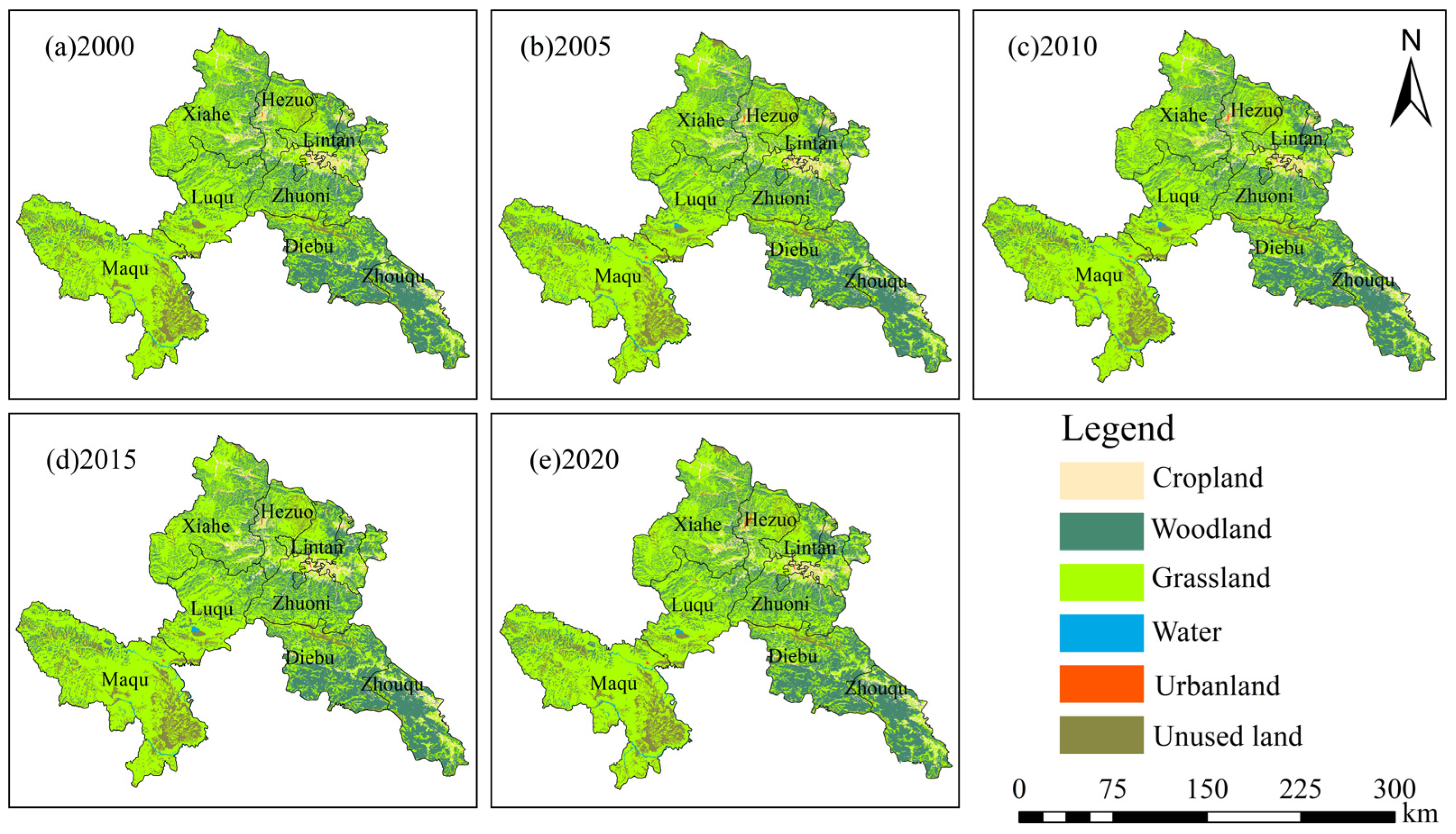
The landscape composition of Gannan is stable from 2000 to 2020 (

Table 5. Dynamic degree of various landscape types in GN from 2000 to 2020.

Period	Landscape Type	Grassland	Urban Land	Cropland	Woodland	Water	Unused Land
2000	Area/km2	20,800.84	106.37	1699.15	11,213.17	217.45	2656.72
	Proportion/%	56.69	0.29	4.63	30.56	0.59	7.24
2005	Area/km2	20,882.51	116.14	1635.42	11,231.83	236.22	2591.58
	Proportion/%	56.91	0.32	4.46	30.61	0.64	7.06
2010	Area/km2	20,764.23	143.39	1636.77	11,240.61	278.89	2629.81
	Proportion/%	56.59	0.39	4.46	30.63	0.76	7.17
2015	Area/km2	20,754.81	178.01	1607.35	11,234.21	286.02	2633.29
	Proportion/%	56.56	0.49	4.38	30.62	0.78	7.18
2020	Area/km2	20,822.25	181.44	1589.86	11,258.95	264.4	2576.8
	Proportion/%	56.75	0.49	4.33	30.68	0.72	7.02
Dynamic Attitude/%	2000–2020	0.01	3.53	−0.32	0.02	1.08	−0.15

and Figure 3) consisting mainly of grassland, woodland, unused land, cropland, urban land, and water. Grasslands are the most extensive of all landscape types, covering more than 56% of the GN’s total area. Woodlands occupy over 30% of the total area. Unused lands and water constitute a minimal portion, less than 1%.

With respect to spatial distribution characteristics, grasslands are predominantly found in the west, where the plains and plateaus are situated. Woodlands are mainly distributed in the mountainous areas in the south and east. Urban lands are concentrated in counties and cities, with unused lands scattered around them. Water mainly belongs to the Yellow River and the Taohe basin, interspersed and distributed in Gannan. Unused lands are scattered in Maqu.

Among various landscape types, croplands exhibited the most substantial change, illustrating a consistent downward trend (109.29 km²), followed by unused lands (79.92 km²). Urban lands experienced the most extensive expansion (75.07 km²), demonstrating a continuous increasing trend. Grasslands presented the smallest change in area (22.41 km²). In terms of land use dynamics, urban lands and water bodies displayed the highest values of change dynamics, which can be attributed to their relatively small base areas, resulting in more pronounced relative changes.

3.1.2. Landscape Composition Map Trajectory Analysis

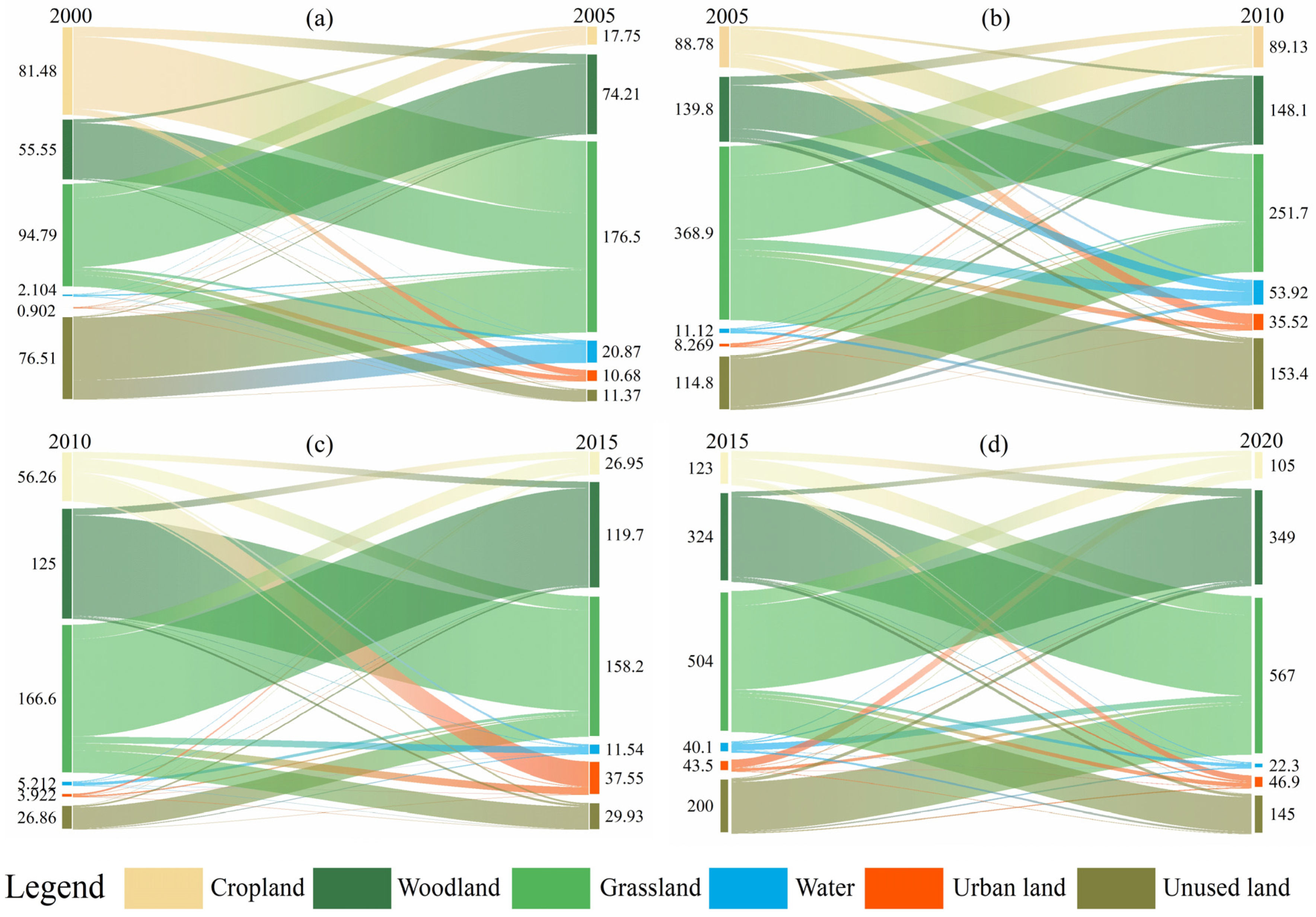
Based on the landscape type shift analysis, the results for the four periods (2000–2005, 2005–2010, 2010–2015, and 2015–2020) displayed the following.

From 2000 to 2005, the largest areas of landscape area transferred out and transferred in were both grasslands (Figure 4), 94.79 km² and 176.5 km², respectively (

Table 6. Landscape type shift table for GN from 2000 to 2020.

2000–2005			2005–2010			2010–2015			2015–2020
Code	Area/km2	Proportion/%	Code	Area/km2	Proportion/%	Code	Area/km2	Proportion/%	Code	Area/km2	Proportion/%
1 → 3	66.42	21.33	3 → 6	136.70	18.68	2 → 3	113.60	29.59	3 → 2	301.46	24.58
3 → 2	63.66	20.45	3 → 2	134.84	18.43	3 → 2	109.54	28.53	2 → 3	288.52	23.52
6 → 3	57.55	18.49	6 → 3	101.68	13.90	1 → 5	28.42	7.40	6 → 3	176.44	14.39
2 → 3	50.87	16.34	2 → 3	91.83	12.55	3 → 6	25.09	6.54	3 → 6	124.00	10.11
6 → 4	17.64	5.67	3 → 1	63.10	8.62	6 → 3	23.90	6.23	1 → 3	68.38	5.58
3 → 1	13.51	4.34	1 → 3	52.68	7.20	3 → 1	16.23	4.23	3 → 1	52.58	4.29

Note: The numbers 1 through 6 correspond to cropland, woodland, grassland, water, urban land, and unused land, respectively. Code 1 → 3 signifies the conversion of cropland to grassland, with other codes following the same below.

). Croplands represent the landscape type with the most significant area transferred to grasslands, comprising 21.334% of the total transferred area. Grasslands transfer to woodlands account for the largest share, constituting 20.446%. This transfer primarily occurs in Xiahe, Zhuoni, and Maqu counties (Figure 5).

From 2005 to 2010, the largest areas of landscape transferred out and transferred in were both grasslands, 368.9 km² and 251.7 km², respectively. The shift from unused lands and woodlands to grasslands is large, accounting for 13.896% and 12.550% of all transferred areas. Grasslands are also mainly shifted to unused lands and woodlands, representing 18.683%, and 18.428% of all transferred areas, respectively. Areas of transfer are mainly in Luqu, Zhuoni, and Diebu counties.

From 2010 to 2015, grasslands experienced the largest net transfer of area, both in terms of area transferred out and area transferred in, with 166.6 km² and 158.2 km², respectively. The majority of the area transferred into grasslands came from woodlands, which represented 29.592% of all areas transferred. The conversion of grasslands to woodlands accounted for 28.533% of all areas transferred. Transferred regions are mainly located in Xiahe, Lintan, and Maqu counties. Additionally, Figure 5c clearly exhibits the large-scale expansion of urban lands in Hezuo, with the expansion area originating from croplands.

From 2015 to 2020, grasslands consistently had the largest area of landscape transfer both into and out of it, at 504 km² and 567 km², respectively. As in 2010 to 2015, the area of grasslands transferred in is predominantly from woodlands, and the area transferred out is also predominantly shifted to woodlands. They accounted for 23.524% and 24.579% of all areas transferred, respectively. Transferred regions are also concentrated in Luqu, Zhuoni, and Diebu counties.

In conclusion, from 2000 to 2020, landscape changes occur mainly between grasslands and woodlands, with a clear concentration in Xiahe, Zhuoni, Maqu, and Diebu. Grasslands to woodlands had the largest area of landscape type transfer, with more than 18% of the area transferred in each study period (Table 6).

3.2. Results of Landscape Pattern Features Analysis

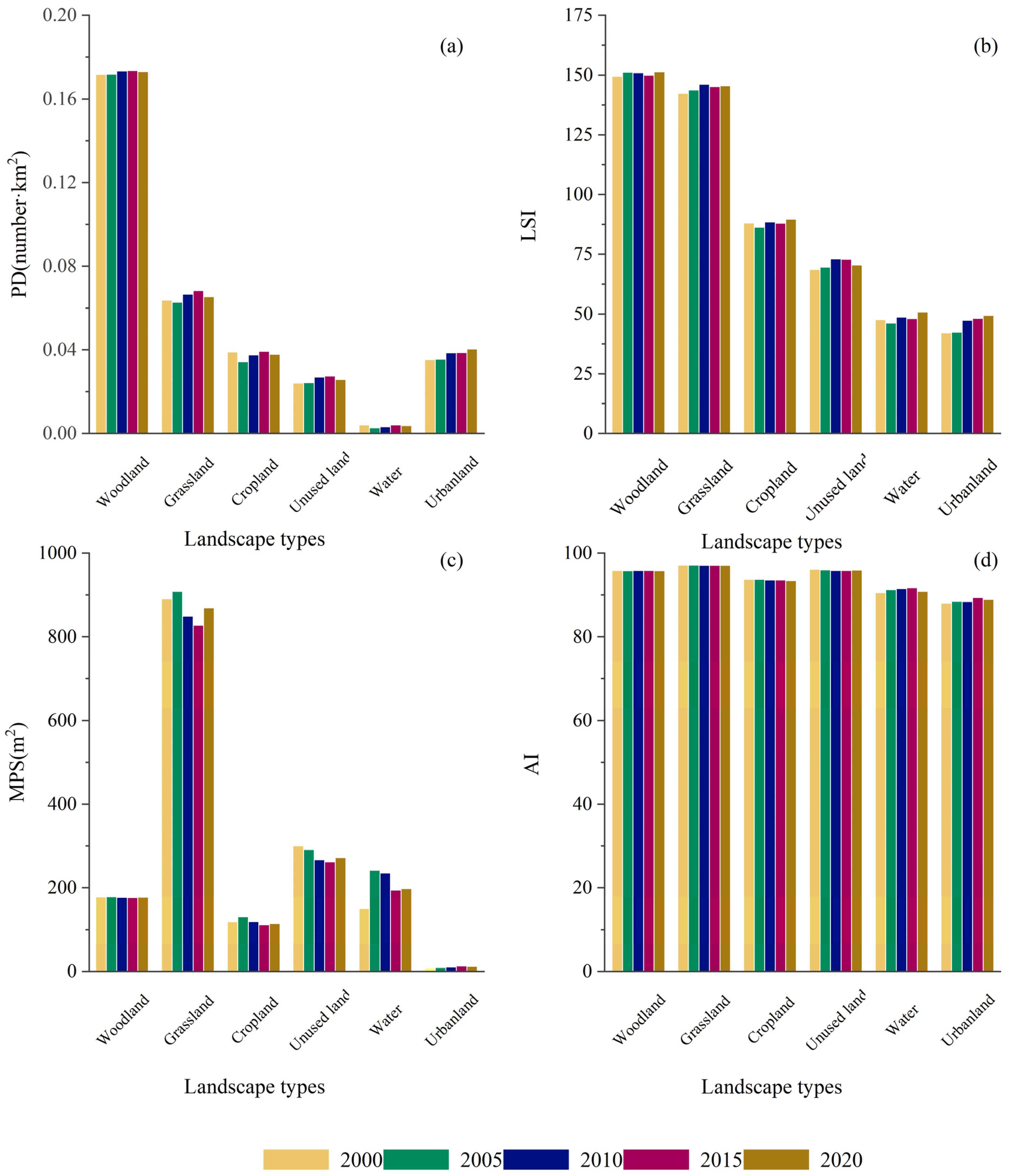
Landscape pattern features in Gannan have changed over the past 20 years (Figure 6). According to patch density (PD), the value of woodland reflected a single-peak fluctuation and reached a maximum value of 0.175 in 2015 (Figure 6a). The trend of unused land and woodland was consistent. All other landscape pattern types had PD values < 0.1. The PD values for grassland exhibited a trend of decrease–increase–decrease, with a peak of 0.0683 reached again in 2015, and the trend in values for cropland and water was consistent with it. The value for urban land, on the other hand, illustrated a continuous upward trend, reaching a maximum value of 0.0403 in 2020.

The LSI values in Gannan fluctuated less during the study period, but all landscape types revealed an increasing trend in LSI values (Figure 6b). Specifically, woodland has the highest LSI value, followed by grassland, with both types having LSI values above 140. This constituted that the length of the woodland and grassland boundaries is long, which may be related to the increase in area. However, human activity may also have fragmented the patches.

The MPS for woodland, grassland, cropland, and water was basically the same, all exhibited an increasing–decreasing–increasing trend (Figure 6c). However, the values of woodland, grassland, and cropland all decreased. Additionally, the MPS value for unused land declined by 28.2763 m², except for the overall increase in the values of MPS for water and urban land. Among them, grassland had the largest value and the largest landscape patch size with yearly values, all >800 m², with the best internal connectivity.

The AI values for each landscape type did not differ much and did not vary much from period to period, being around 90 (Figure 6d). Among them, grassland has the largest value, indicating strong connectivity between grassland patches and a high degree of ecological stability, while urban land has a low degree of landscape aggregation due to a high degree of human activity impacts.

In summary, PD exhibited a unimodal fluctuation, peaking in 2015. LSI demonstrated a consistent upward trajectory across all landscape types. Except for water and urban land, MPS displayed a declining trend. AI remained stable throughout the study period. Notably, woodland registered the highest PD and LSI values among all landscape types, whereas grassland exhibited the largest MPS and highest AI values.

3.3. Spatiotemporal Pattern of LERI

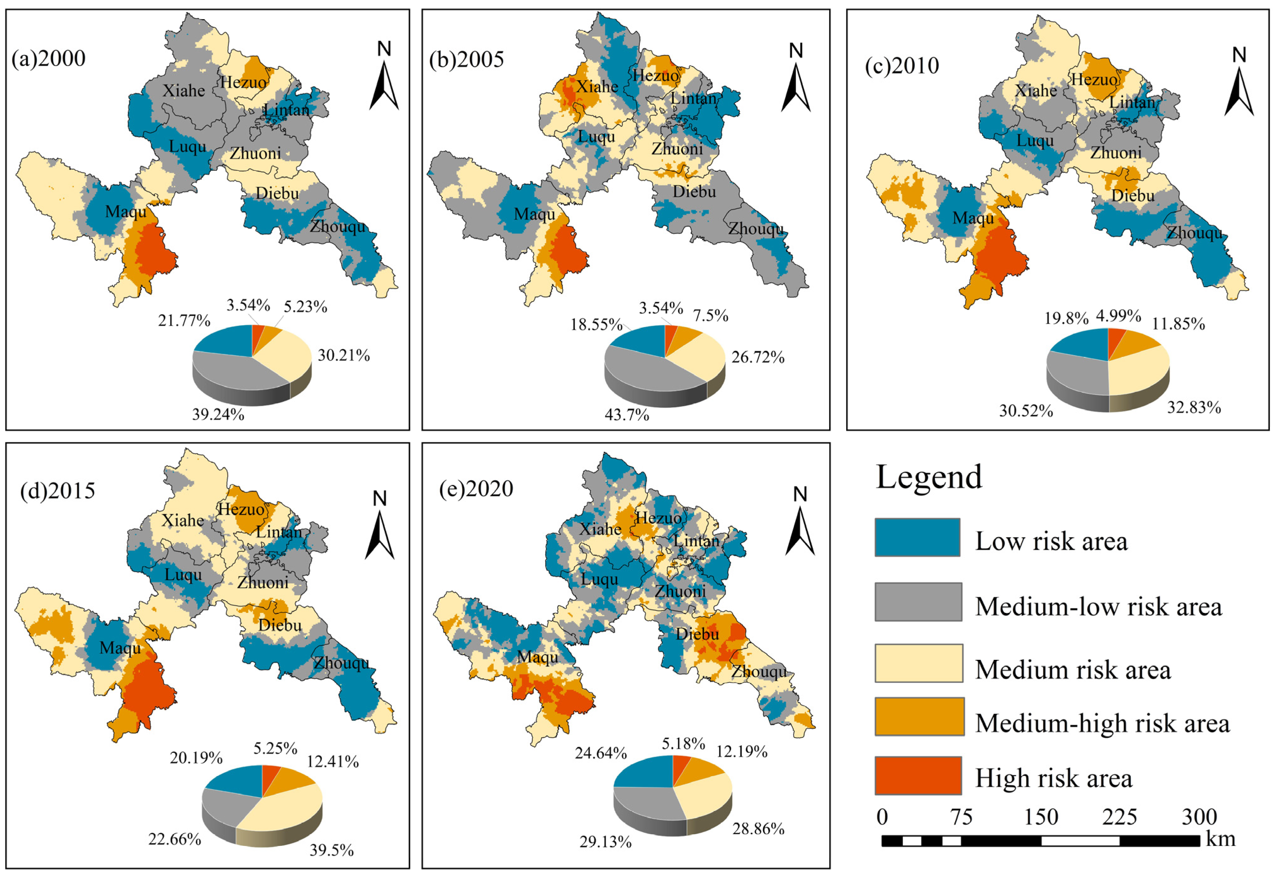
The results of the LERI assessment of GN were analyzed by standardizing and classified into five levels: low risk area (LERI ≤ 0.48), medium-low risk area (0.48 < LERI ≤ 0.53), medium risk area (0.53 < LERI ≤ 0.58), medium-high risk area (0.58 < LERI ≤ 0.65), and high risk area (LERI > 0.65). Figure 7 demonstrated the spatial distribution across the five levels of LERI.

The spatial variation in LERI is notable, with high-risk zones exhibiting a pattern of progression from the southwest to the northeast. Between 2000 and 2020, the combined areas of the medium-risk and medium–low-risk zones comprised approximately 60%, mainly in Luqu, Xiahe, Lintan, and Zhouqu. The low-risk area rose from 21.77% to 24.64%, primarily in Maqu, Luqu, and Lintan. At the same time, the high-risk and medium–high-risk areas remained relatively low, approximately 10%, but reflected an upward trend, increasing by 1.64% and 6.96%, respectively, and were scattered in areas such as eastern Maqu, urban areas of Hezuo, and central Diebu.

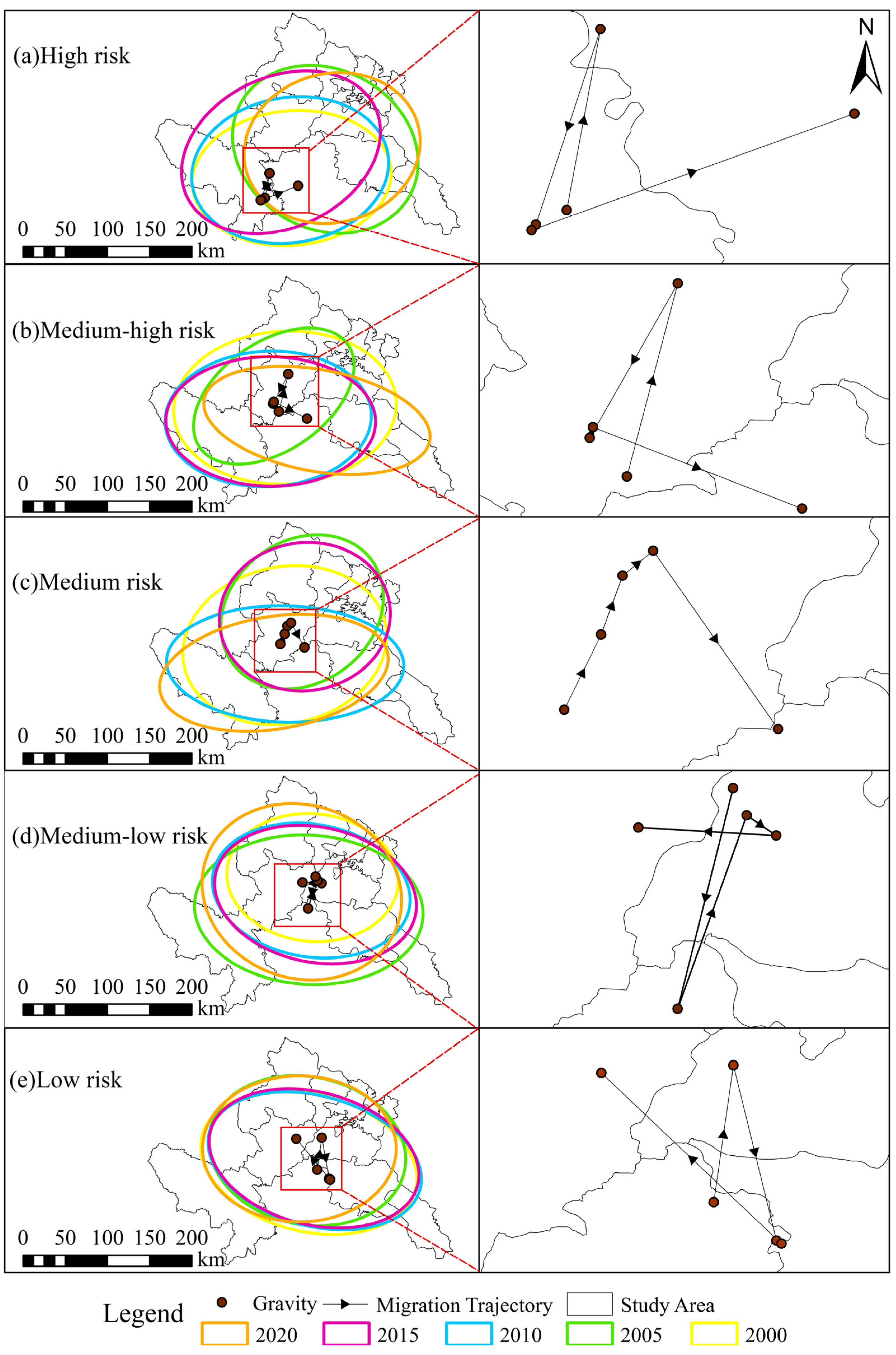
To delve deeper into the transitions of LER, we conducted centroid migration and directional distribution analyses for each risk level using SDE (Figure 8,

Table 7. SDE parameters of LER in GN from 2000 to 2020.

Type	Year	X-Axis	Y-Axis	Direction Angle/°
Low risk	2000	130,547.21	83,657.33	104.64
	2005	117,764.87	90,213.67	102.53
	2010	129,501.61	79,161.70	105.92
	2015	127,037.64	80,664.52	105.38
	2020	114,760.41	89,218.46	89.57
M-low risk	2000	101,715.88	75,211.79	94.98
	2005	135,541.49	88,044.18	93.45
	2010	118,064.05	78,261.24	99.56
	2015	120,897.79	79,742.84	101.32
	2020	119,921.77	102,087.66	108.84
M risk	2000	136,767.68	68,540.20	79.86
	2005	122,043.11	95,455.73	91.05
	2010	104,047.91	85,676.25	47.96
	2015	101,700.43	90,420.98	79.34
	2020	136,767.68	68,540.20	79.86
M-high risk	2000	132,028.37	93,328.60	85.82
	2005	108,059.64	65,598.19	52.99
	2010	122,150.02	82,577.40	86.47
	2015	124,151.14	78,956.79	89.92
	2020	135,911.05	61,929.13	100.52
High risk	2000	117,975.56	81,951.92	83.93
	2005	114,912.91	96,648.85	122.59
	2010	117,371.20	88,377.94	79.29
	2015	124,173.96	91,140.96	61.77
	2020	105,564.51	90,658.66	72.11

). While the centroid of high-risk areas clustered in the southwest of GN, other risk levels exhibited relatively uniform centroid distribution across GN. The southwestward bias of high-risk centroids primarily resulted from the extensive high-risk coverage east of Maqu. Centroids of low risk and medium-low risk areas shifted westward, whereas those of medium risk, medium–high risk, and high risk areas migrated eastward.

Regarding directional evolution (2000–2020), high risk, medium–low risk, and low risk areas consistently maintained a southwest–northeast-oriented major axes. Their x axes shortened with reduced dispersion. Conversely, medium–high risk areas displayed a northward shift in orientation over the period from 2000 to 2005, with axis direction changing from 85.82° to 52.99°. From 2005 to 2020, their primary axis orientation transitioned from southwest–northeast to southeast–northwest, reaching 100.52°. This coincided with X axis elongation and increased dispersion. Medium risk areas shifted northward between 2000 and 2005 (76.02° to 91.05°), then southward in the period 2005–2010 (91.05° to 47.96°), and finally northward during the period 2010–2020 (47.96° to 79.86°), accompanied by X axis lengthening and enhanced dispersion.

Collectively, high-risk areas developed with southwestern bias yet demonstrated a northeastward migration trend from 2000 to 2020. Low risk and moderate–low-risk areas exhibited pronounced westward development trends. These three risk levels exhibited decreased dispersion. In contrast, medium risk and medium–high risk areas developed northward with increased dispersion.

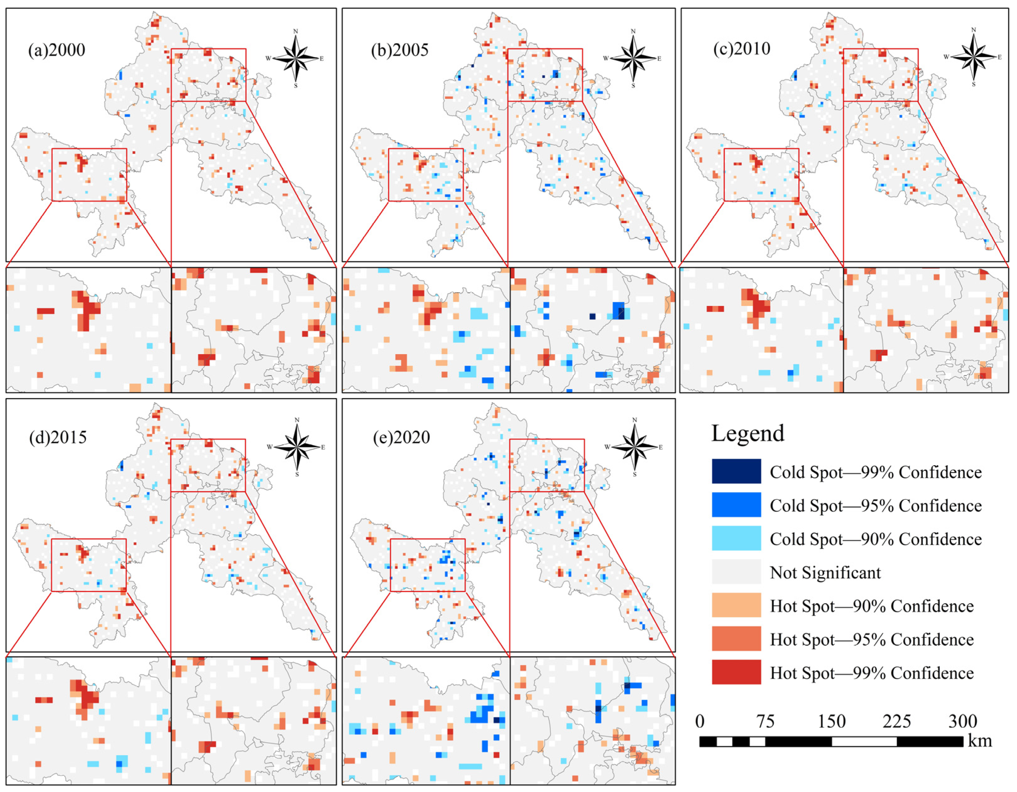
The spatial distribution of LER cold and hot spots was analyzed utilizing the Hot Spot Analysis tool (Getis-Ord Gi*) in ArcGIS, as illustrated in Figure 9. The mean p-value for the hot spot areas (Z(Gi) > 1.9) was 0.02, while that for the cold spot areas (Z(Gi) < −1.9) was 0.03, both demonstrating statistical spatial significance. The LER hot spots in the GN region were predominantly concentrated in urban areas, such as the urban core of Hezuo, Oula Town in Maqu, and the urban zones of Luqu and Zhuoni. Anthropogenic construction of towns and industrial parks has exerted substantial ecological pressure. In contrast, cold spots were less abundant than hot spots and were primarily located within ecological protection zones and plateau wetland areas. Furthermore, a comparison of the LER cold and hot spot distributions across the five periods revealed that the number of hot spot clusters in 2020 was significantly lower than in the previous four periods, whereas the number of cold spot clusters was markedly higher. This denotes a positive trend in the LER status of the GN region.

3.4. Landscape Ecological Risk Driver Analysis

3.4.1. Detection Factor Influence

The factor detector was employed to assess the extent of each factor’s influence on the LERI. By determining the q-value for factors, we determined the force of each factor from 2000 to 2020 (

Table 8. Single factor detection results of LERI drivers from 2000 to 2020.

Factor	Code	q Statistic					p Value
		2000	2005	2010	2015	2020	2000	2005	2010	2015	2020
Population density	X1	0.02	0.04	0.02	0.02	0.00	0.00	0.00	0.00	0.00	0.99
Cumulative annual precipitation	X2	0.09	0.16	0.06	0.10	0.24	0.00	0.00	0.00	0.00	0.00
Elevation	X3	0.14	0.18	0.16	0.16	0.02	0.00	0.00	0.00	0.00	0.00
Slope	X4	0.08	0.07	0.09	0.09	0.01	0.00	0.00	0.00	0.00	0.00
Annual average temperature	X5	0.15	0.14	0.15	0.16	0.03	0.00	0.00	0.00	0.00	0.00
Distance from road	X6	0.01	0.01	0.01	0.01	0.01	0.00	0.00	0.00	0.00	0.00
Distance to water	X7	0.00	0.00	0.00	0.00	0.00	0.88	0.65	0.72	0.69	1.00
GDP	X8	0.11	0.09	0.20	0.13	0.02	0.00	0.00	0.00	0.00	0.00

).

The factors were ranked in descending order of their influence on LERI: elevation > annual average temperature > cumulative annual precipitation > GDP > slope > population density > distance from road > distance to water (Table 8). The results displayed that all independent variables except X7 distance to water and X1 population density in 2020 passed the 0.01 level of significant test, proving that the results are credible.

Table 8 implied that the q-values for elevation and annual average temperature were larger. The spatial pattern of the effect of altitude on LERI was generally the largest, with the first q-value in both 2005 (0.18) and 2015 (0.15), showing a fluctuating downward trend. Secondly, the spatial pattern of LERI was slightly less influenced by annual average temperature than elevation, which was the first in 2000 (0.14) and had q-values above 0.138 in all three periods from 2005 to 2015. The next influential factors are cumulative annual precipitation and GDP, with 2020 cumulative annual precipitation having the highest impact value (0.24), 2010 GDP having the highest impact value (0.20).

3.4.2. Analysis of Interaction Between Factors

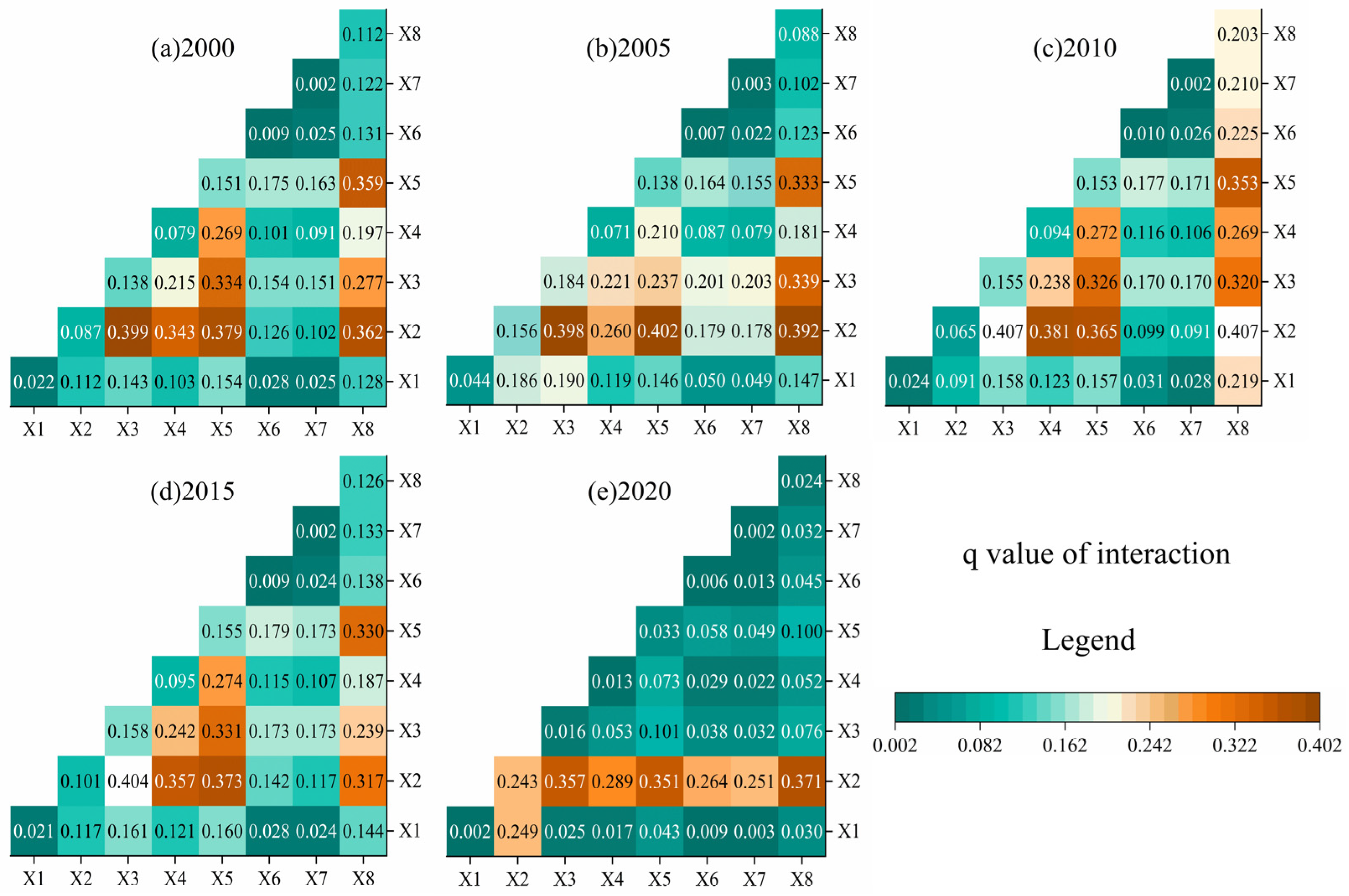
The interaction detection results (Figure 10) revealed that factor interactions contributed to LERI through both bidirectional and nonlinear enhancements. The interaction effect exceeded the combined effects of the individual factors, suggesting mutual reinforcement among the driving factors.

From the heat map, we can see that the interplay between elevation and cumulative annual precipitation had the greatest impact on LERI, exceeding 0.35. Interaction was greater than the sum of the two, and their interactions were in the top two places. Second, the interactions of annual average temperature with annual precipitation (>0.35) and GDP with annual precipitation (>0.31) also had a significant effect on LERI, with interactions being greater than the sum of the two.

In summary, there are significant synergistic effects among the different influencing factors of LERI. Their collective influence is greater than that of individual factors. Notably, the interactive effects of precipitation and elevation play a particularly prominent role.

4. Discussion

4.1. Landscape Pattern Dynamics Analysis

The results revealed that the proportions of landscape types and their areas in GN remained stable, with the ratio of area change across landscape types being less than 1%. These results are likely associated with the regional economic structure [55]. Specifically, traditional agriculture, animal husbandry, and tourism are the dominant industries in GN. These industries usually have a low impact on the environment and land [56]. Therefore, the industrial structure of the region is conducive to maintaining a stable landscape structure. Additionally, agricultural or livestock production practices, such as rotational grazing or fallow farming, help to restore soil fertility [57], which is also beneficial to maintaining landscape stability.

Additionally, the policies to protect ecological stability may explain this result. To preserve the ecological balance, several policies have been implemented by both national and local governments [58]. For instance, policies, such as fencing and sealing, have been formulated to favor grasslands restoration [59]. Furthermore, a number of ecological protection zones have been established, including the Taohe River, Gahai-Zecho, and Yellow River Shouqu reserves, and so on [60]. These nature reserves play an important role in curbing degradation of the ecology by reducing human interference [61]. Notably, the key species restoration efforts in Gahai Lake resulted in more than tenfold increases in both black-necked crane and black stork populations over the 2004–2009 period [62].

Moreover, human disturbance to the landscape is an important factor. The human disturbance index at high elevation area (≥3000 m) is only one-third that of low elevation area (<3000 m) [51]. Much of GN is over 3000 m above sea level, with average annual temperatures ranging from 5 to 10 °C, thus limiting human activities [63]. This benefits landscape stability [64]. Besides, with warmer temperatures and increased precipitation, vegetation growth in the region accelerates, contributing to the development of a stable landscape structure [65]. Furthermore, our results are consistent with previous studies, demonstrating both the structural stability of the landscape in GN and the beneficial effects of woodland and grassland landscapes [27,32].

We also found that changes in landscape patterns occurred mainly between woodlands and grasslands, which were mainly concentrated in the southwest and north of GN. This is related to the Physiological advantages of plants. The woody species exhibit superior root-system development and faster colonization rates on slopes with favorable edaphic-hydrological conditions than the grassland [66]. Furthermore, the landscape types of GN are dominated by grassland landscape and woodland landscape. Consequently, the expansion of woodland landscapes inevitably leads to the reduction of grassland landscape [67]. Moreover, precipitation is mainly concentrated in the river valleys and slopes [31]. Favorable hydrothermal conditions support the expansion of vegetation [68]. The woodland-grassland interspersed zones in the study area are mainly located in the areas mentioned above, which further supports our findings.

Additionally, protection policies on forest land may accelerate the expansion of woodland landscapes [69]. As a typical alpine meadow area, the planning of economic forests and the construction of forest parks will inevitably accelerate the natural succession of grassland landscape to woodland landscape [70]. A total of 10.24 million hm² of various economic forests, six national forest parks, four provincial forest parks, and more than thirty other forest tourist attractions have been built in the study area [33]. Furthermore, the 2023 forest conservation effectiveness report from Diebu County indicates a 12% expansion of protected forest area since 2018, significantly exceeding the 6.7% growth observed in non-protected zones. Therefore, we discovered that the expanded woodland landscape mainly comes from the grassland landscape. This is consistent with the findings of Luo [27].

4.2. Response of LER Change to Landscape Pattern

The trend of LER distribution in the GN is high in the southwest and low in the northeast, and the gravity of the high-risk area is in the southwestern part of GN. This may be related to the differences between grassland and woodland vegetation in terms of growth structure. The root systems of grassland plants are generally less than 20 cm deep, characterized by a high proportion of fine roots and low mechanical strength [71]. In contrast, the woodland landscape has a dense and deep root system with high mechanical strength [72]. As opposed to grassland landscape, woodland landscapes show greater resistance to disturbance [73]. We previously found that grassland landscape is mainly distributed in the west and woodland landscape is concentrated in the east. Previous studies on landscape ecological risk in Saihanba have concluded that an increase in the proportion of woodlands leads to a decrease in LER [74]. These results further support our findings.

Furthermore, from the perspective of landscape pattern indices, we also found that grassland landscape in GN exhibited higher MPS and AI values compared to woodland landscape. In contrast, the grassland landscape had lower PD and LSI values than the woodland landscape. That is, the woodland landscape had more diverse shapes and ecological processes compared to grassland landscape [32]. Thus, the LER distribution is high in the southwest and low in the northeast in GN. Concurrently, concentrated unused land areas in southwestern GN exhibit sparse grasslands coverage and limited livestock density, which negatively impacts patch connectivity [75]. In contrast, eastern GN’s aggregated distribution of grasslands and wetlands maintains lower vegetation fragmentation levels.

Elevation may be another key influence factor. It is well known that high elevation areas have poorer hydrothermal conditions and higher LER than low elevation areas [76]. The high elevation areas with fragile natural backgrounds can lead to vegetation degradation when disturbed by anthropogenic disturbances or climate-induced hazards [77]. The GN’s orographic pattern is a descending gradient from southwestern plateaus to northeastern hills, with the highest average elevation (3700 m) in Maqu [75]. Furthermore, according to statistics from the Gansu Provincial Grassland General Station in 2018, approximately 90% of the natural grasslands in Maqu was degraded to varying degrees. The degradation was mainly caused by overgrazing or rodent and insect infestation. Meanwhile, the area of desertification in Maqu’s grasslands had reached 53,333 hectares by that year [78]. Previous studies have also revealed that the grasslands in Maqu has exhibited increased sensitivity to climate change, leading to a higher risk of grasslands degradation [79]. In 2000, the actual stocking rate of Maqu exceeded the theoretical stocking rate by 800,000 sheep units [80]. In 2010, the overloading rate remained at 35%. In addition, illegal mining also affects the LER [81]. Thus, the gravity of the high-risk area is focused on the southwestern part of GN.

We observed that GDP is a significant risk-driving factor, second only to topographic and climatic variables, despite urban lands accounting for less than 0.5% of the total area. This phenomenon is closely related to the economic structure of GN. Its GDP is primarily derived from characteristic animal husbandry and eco-tourism, rather than traditional industrial or real estate expansion [82,83]. High-value-added activities, such as livestock sales, animal product processing, and tourism consumption, are highly concentrated in urban areas and industrial parks, resulting in intensive land use and high economic output intensity [84,85]. Thus, even with limited land development scale, GDP still exhibits considerable explanatory power. Furthermore, LER hotspot analysis further indicates that high-risk areas are concentrated around urban zones and industrial parks [25]. These areas act as “point sources” of intense human disturbance, dispersing ecological impacts to broader regions through transportation corridors, and radiation effects, thereby influencing the overall risk pattern [86]. Consequently, as an effective indicator of the intensity of human economic activities, GDP significantly shapes the distribution of landscape ecological risk in GN.

4.3. Driving Mechanism of LER Pattern

Our study confirms that natural factors are the main drivers of LER patterns. From a single-factor perspective, elevation is the most influential factor. In high altitude areas, the main factors affecting LER are grasslands desertification–matrix problem and grasslands degradation–rat damage problem [87,88]. Soil organic matter content at high elevations is less than 2%, while at lower elevations, it can be as high as 8–10% [89]. As a result of this difference, high elevation areas in the southwest have lower levels of land cover than lower elevations due to this difference. However, the burrow networks and surface collapses caused by rodent damage can destroy the grass mat layer and form erosion gullies [90]. Therefore, soil depletion and rodent infestation significantly impact LER in high-altitude regions [91]. Moreover, elevation also affects extreme weather events [92] and the intensity of human disturbances [93]. Ecological restoration is more difficult at high altitudes than at low altitudes [94]. Therefore, elevation is a key factor influencing LER patterns. This conclusion is consistent with our previous findings.

From a multi-factorial perspective, precipitation and elevation are the main drivers of LER. This may be because precipitation and elevation together influence the hydrothermal conditions of ecosystems [95]. Annual precipitation at high elevation (such as Maqu and Luqu) can exceed 800 mm, but low temperatures limit the efficient use of water [96]. As a result, the development of forages with high water requirements (such as Poa pratensis and alfalfa) is restricted at high elevation [97]. Thus, precipitation and elevation interactions influence each other in the distribution of vegetation. In addition, global warming has had an impact on the water–heat balance of the global precipitation network. From 2000 to 2020, the rate of warming in the higher elevation regions of the GN will increase by 0.36 °C per decade [98], which is higher than the national average. This leads to degradation of permafrost and shorter snowpack periods, exacerbating the fragmentation and erosion of alpine meadows. Therefore, the combination of precipitation and elevation is the primary driver for the region.

Another possible explanation is that the coupling of precipitation and elevation influences erosion and geological hazards. Precipitation-induced runoff produces greater scouring forces at high elevation areas where the average slopes are greater than 25° [99]. Soil erosion modulus at high elevation can be up to 5000 tons/km²-year [100]. The interaction between precipitation intensity and terrain slope greatly increases erosion and ecological risk. In addition, snowmelt runoff in the spring and permafrost degradation at high elevation threaten the LER by increasing the potential for spring flooding and mudslides.

4.4. Limitations and Future Work Directions

We utilized a 12 km × 12 km grid as the study scale and employed the natural breakpoint method for LER zoning. Compared to the county scale, the grid scale offers a more precise analysis by minimizing the interference of administrative boundaries. Moreover, using the county scale in studies may homogenize data within the county may fail to capture the detailed distribution of high-risk areas, such as erosion gullies and fragmented habitats. Therefore, the grid scale for evaluating ecological risk has better applicability than the county scale [14]. There is also some uncertainty in the study. This uncertainty mainly comes from cloud cover, atmospheric conditions, or sensor limitations that may result from remote sensing. Furthermore, the study period spans from 2000 to 2020. Moving forward, more comprehensive research on long-term trends and future projections based on updated data would be beneficial for guiding the prospective development of GN.

To advance the green development of GN, we hereby propose the following recommendations:

(1)

Urbanization Challenges: with ongoing urbanization, GN faces various challenges resulting from social development and the growth of population centers, including cities and district towns. Thus, it is crucial to ensure a harmonious coexistence between urbanization and the ecological environment. Future development plans must fully integrate ecological preservation into urban construction and management processes to safeguard the environment. Future economic activities in Hezuo and other urban areas should prioritize transitioning toward eco-friendly industries. This includes increasing the proportion of clean energy utilization and developing derivative products, such as yak-derived goods and highland barley liquor, to reduce direct dependence on grasslands.

(2)

Ecological Restoration in Low-population Areas: in sparsely populated alpine meadows and regions with concentrated unused lands, scientific methods should be employed for ecological restoration, monitoring, and management. For instance, drone surveillance, “one household, one code” management of pastures, and mixed sowing of grass seeds for the management of grasslands degradation could be effective measures. Particular attention must be directed to high-risk zones like western Maqu County.

(3)

Sustainable Ecological Reconstruction: at present, artificial restoration efforts in GN primarily focus on vegetation planting. However, reliance on a single species may destabilize the ecosystem. Future ecological reconstruction initiatives should be grounded in the study of vegetation species composition within grassland and woodland landscapes. Scientifically planned vegetation planting can help achieve more effective and sustainable ecological protection. For instance, in LER-degraded areas of central Diebu county, ecological restoration should prioritize zones characterized by steep slopes and pronounced edge effects.

5. Conclusions

This study analyzed changes in landscape patterns and LER from 2000 to 2020 and explored the causes of LER.

The results of the study implied the following: (1) From 2000 to 2020, the landscape composition of GN remains stable, with grasslands and woodlands being the dominant landform types, both showing an upward trend. Grasslands were primarily found on the western plateau, while woodlands predominated in the eastern and southern mountainous regions. Landscape changes primarily occurred between the grassland and the woodland, with notable concentrations in Xiahe, Zhuoni, Maqu, and Diebu. (2) PD and LSI in the study area reflect an upward trend, AI remains stable, and MPS for major landscape types, such as woodlands and grasslands, illustrates a declining trend. (3) LER is decreasing, with high-risk regions primarily in eastern Maqu, Hezuo, and central Diebu. The centers of low and medium–low risk areas have migrated westward, whereas centers of medium–high and high-risk regions have shifted eastward. (4) Among the natural and social factors influencing LER, altitude exerts the greatest influence, with even stronger interactions among different factors. Precipitation demonstrates the greatest interaction with other factors. Natural factors, such as climate and topography, are more powerful forces on LER than socio-economic factors. Consequently, protective measures, such as fencing and drone-assisted monitoring should be implemented in high risk regions, including western Maqu County. Future research should integrate multi-source spatial data to examine landscape ecological risk (LER) dynamics and predictive research.

References

1. Lecina-Diaz, J.; Senf, C.; Grünig, M.; Seidl, R. Ecosystem Services at Risk from Disturbance in Europe’s Forests. Glob. Change Biol. 2024, 30, e17242. [Google Scholar] [CrossRef] [PubMed]
2. Guo, H. The SDGSAT-1 Mission and Its Role in Monitoring SDG Indicators. Remote Sens. Environ. 2025, 328, 114885. [Google Scholar] [CrossRef]
3. Deng, G.; Jiang, H.; Zhu, S.; Wen, Y.; He, C.; Wang, X.; Sheng, L.; Guo, Y.; Cao, Y. Projecting the Response of Ecological Risk to Land Use/Land Cover Change in Ecologically Fragile Regions. Sci. Total Environ. 2024, 914, 169908. [Google Scholar] [CrossRef]
4. Li, W.; Liu, Y.; Lin, Q.; Wu, X.; Hao, J.; Zhou, Z.; Zhang, X. Identification of Ecological Security Pattern in the Qinghai-Tibet Plateau. Ecol. Indic. 2025, 170, 113057. [Google Scholar] [CrossRef]
5. Wang, S.; Tan, X.; Fan, F. Landscape Ecological Risk Assessment and Impact Factor Analysis of the Qinghai–Tibetan Plateau. Remote Sens. 2022, 14, 4726. [Google Scholar] [CrossRef]
6. Hunsaker, C.T.; Graham, R.L.; Suter, G.W.; O’Neill, R.V.; Barnthouse, L.W.; Gardner, R.H. Assessing Ecological Risk on a Regional Scale. Environ. Manag. 1990, 14, 325–332. [Google Scholar] [CrossRef]
7. Du, Z.; Ji, X.; Liu, J.; Zhao, W.; He, Z.; Jiang, J.; Yang, Q.; Zhao, L.; Gao, J. Ecological Health Assessment of Tibetan Alpine Grasslands in Gannan Using Remote Sensed Ecological Indicators. Geo-Spat. Inf. Sci. 2025, 28, 246–264. [Google Scholar] [CrossRef]
8. Wu, J.; Zhu, Q.; Qiao, N.; Wang, Z.; Sha, W.; Luo, K.; Wang, H.; Feng, Z. Ecological Risk Assessment of Coal Mine Area Based on “Source-Sink” Landscape Theory—A Case Study of Pingshuo Mining Area. J. Clean. Prod. 2021, 295, 126371. [Google Scholar] [CrossRef]
9. Guo, K.; Kuai, X.; Chen, Y.; Qi, L.; Zhang, L.; Liu, Y. Risk Assessment of Land Ecology on a Regional Scale: Application of the Relative Risk Model to the Mining City of Daye, China. Hum. Ecol. Risk Assess. Int. J. 2017, 23, 550–574. [Google Scholar] [CrossRef]
10. Xu, W.; Wang, J.; Zhang, M.; Li, S. Construction of Landscape Ecological Network Based on Landscape Ecological Risk Assessment in a Large-Scale Opencast Coal Mine Area. J. Clean. Prod. 2021, 286, 125523. [Google Scholar] [CrossRef]
11. Li, T.; Xiong, K.; Yang, S.; Liu, H.; Qin, Y.; Wang, Z. Progress and Prospects of Forest Ecological Asset Research. Sustainability 2021, 14, 395. [Google Scholar] [CrossRef]
12. Li, S.; Tu, B.; Zhang, Z.; Wang, L.; Zhang, Z.; Che, X.; Wang, Z. Exploring New Methods for Assessing Landscape Ecological Risk in Key Basin. J. Clean. Prod. 2024, 461, 142633. [Google Scholar] [CrossRef]
13. Peng, Y.; Cheng, W.; Xu, X.; Song, H. Analysis and Prediction of the Spatiotemporal Characteristics of Land-Use Ecological Risk and Carbon Storage in Wuhan Metropolitan Area. Ecol. Indic. 2024, 158, 111432. [Google Scholar] [CrossRef]
14. Ju, H.; Niu, C.; Zhang, S.; Jiang, W.; Zhang, Z.; Zhang, X.; Yang, Z.; Cui, Y. Spatiotemporal Patterns and Modifiable Areal Unit Problems of the Landscape Ecological Risk in Coastal Areas: A Case Study of the Shandong Peninsula, China. J. Clean. Prod. 2021, 310, 127522. [Google Scholar] [CrossRef]
15. Du, L.; Dong, C.; Kang, X.; Qian, X.; Gu, L. Spatiotemporal Evolution of Land Cover Changes and Landscape Ecological Risk Assessment in the Yellow River Basin, 2015–2020. J. Environ. Manag. 2023, 332, 117149. [Google Scholar] [CrossRef]
16. Zhang, H.; Zhang, J.; Lv, Z.; Yao, L.; Zhang, N.; Zhang, Q. Spatio-Temporal Assessment of Landscape Ecological Risk and Associated Drivers: A Case Study of the Yellow River Basin in Inner Mongolia. Land 2023, 12, 1114. [Google Scholar] [CrossRef]
17. Wang, J.-F.; Zhang, T.-L.; Fu, B.-J. A Measure of Spatial Stratified Heterogeneity. Ecol. Indic. 2016, 67, 250–256. [Google Scholar] [CrossRef]
18. He, J.; Pan, Z.; Liu, D.; Guo, X. Exploring the Regional Differences of Ecosystem Health and Its Driving Factors in China. Sci. Total Environ. 2019, 673, 553–564. [Google Scholar] [CrossRef]
19. Wang, X.; Sun, Y.; Zhang, L.; Mei, Y. Spatial Variation and Influence Factor Analysis of Soil Heavy Metal as Based on geoDetector. Stoch. Environ. Res. Risk Assess. 2021, 35, 2021–2030. [Google Scholar] [CrossRef]
20. He, X.; Tian, J.; Zhang, Y.; Zhao, Z.; Cai, Z.; Wang, Y. Attribution and Driving Force of Nitrogen Losses from the Taihu Lake Basin by the InVEST and GeoDetector Models. Sci. Rep. 2023, 13, 7440. [Google Scholar] [CrossRef] [PubMed]
21. Xiong, L.; Li, S.; Zou, B.; Peng, F.; Fang, X.; Xue, Y. Long Time-Series Urban Heat Island Monitoring and Driving Factors Analysis Using Remote Sensing and Geodetector. Front. Environ. Sci. 2022, 9, 828230. [Google Scholar] [CrossRef]
22. Gao, J.; Zhu, Y.; Zhao, R.; Sui, H. The Use of Cultivated Land for Multiple Functions in Major Grain-Producing Areas in Northeast China: Spatial-Temporal Pattern and Driving Forces. Land 2022, 11, 1476. [Google Scholar] [CrossRef]
23. Wang, Y.; Xiao, J.; Ma, Y.; Ding, J.; Chen, X.; Ding, Z.; Luo, Y. Persistent and Enhanced Carbon Sequestration Capacity of Alpine Grasslands on Earth’s Third Pole. Sci. Adv. 2023, 9, eade6875. [Google Scholar] [CrossRef] [PubMed]
24. Dong, S. Revitalizing the Grassland on the Qinghai–Tibetan Plateau. Grassl. Res. 2023, 2, 241–250. [Google Scholar] [CrossRef]
25. Ma, Z.; Gao, J.; Liang, T.; He, Z.; Feng, S.; Zhang, X.; Zhang, D. Comprehensive Ecological Risk Changes and Their Relationship with Ecosystem Services of Alpine Grassland in Gannan Prefecture from 2000–2020. Remote Sens. 2024, 16, 2242. [Google Scholar] [CrossRef]
26. Yue, D.; Zeng, J.; Yang, C.; Zou, M.; Li, K.; Chen, G.; Guo, J.; Xu, X.; Meng, X. Ecological Risk Assessment of the Gannan Plateau, Northeastern Tibetan Plateau. J. Mt. Sci. 2018, 15, 1254–1267. [Google Scholar] [CrossRef]
27. Luo, X.; Luo, Y.; Le, F.; Zhang, Y.; Zhang, H.; Zhai, J. Spatiotemporal Variation and Prediction Analysis of Land Use/Land Cover and Ecosystem Service Changes in Gannan, China. Sustainability 2024, 16, 1551. [Google Scholar] [CrossRef]
28. Liu, C.; Li, W.; Xu, J.; Zhou, H.; Wang, W.; Wang, H. Temporal and Spatial Variations of Ecological Security on the Northeastern Tibetan Plateau Integrating Ecosystem Health-Risk-Services Framework. Ecol. Indic. 2024, 158, 111365. [Google Scholar] [CrossRef]
29. Xu, C.; Li, C. Correlation between Landscape Pattern and Net Primary Productivity of Vegetation: A Case Study in the Arid and Semi-Arid Regions of Northwest China. Land 2023, 12, 2004. [Google Scholar] [CrossRef]
30. Jin, X.; Jin, Y.; Mao, X. Ecological Risk Assessment of Cities on the Tibetan Plateau Based on Land Use/Land Cover Changes—Case Study of Delingha City. Ecol. Indic. 2019, 101, 185–191. [Google Scholar] [CrossRef]
31. Wang, C.; Zhang, W.; Zou, S.; Xu, B.; Zhang, Y. Spatiotemporal Heterogeneity of Temperature and Precipitation in Complex Terrain along the Northeastern Margin of the Tibetan Plateau. Atmosphere 2023, 14, 988. [Google Scholar] [CrossRef]
32. Liu, C.; Li, W.; Zhu, G.; Zhou, H.; Yan, H.; Xue, P. Land Use/Land Cover Changes and Their Driving Factors in the Northeastern Tibetan Plateau Based on Geographical Detectors and Google Earth Engine: A Case Study in Gannan Prefecture. Remote Sens. 2020, 12, 3139. [Google Scholar] [CrossRef]
33. Zhao, Y.; Zhang, Q.; Zhang, H.; Huang, S. Spatio-Temporal Patterns and Driving Factors of Green Development Level in Alpine Meadow Regions: A Case Study in Gannan Tibetan Autonomous Prefecture. Ecol. Indic. 2024, 168, 112751. [Google Scholar] [CrossRef]
34. Guo, J.; Shen, B.; Li, H.; Wang, Y.; Tuvshintogtokh, I.; Niu, J.; Potter, M.A.; Li, F.Y. Past Dynamics and Future Prediction of the Impacts of Land Use Cover Change and Climate Change on Landscape Ecological Risk across the Mongolian Plateau. J. Environ. Manag. 2024, 355, 120365. [Google Scholar] [CrossRef]
35. Cuba, N. Research Note: Sankey Diagrams for Visualizing Land Cover Dynamics. Landsc. Urban Plan. 2015, 139, 163–167. [Google Scholar] [CrossRef]
36. Cao, Y.; Dong, B.; Xu, H.; Xu, Z.; Wei, Z.; Lu, Z.; Liu, X. Landscape Ecological Risk Assessment of Chongming Dongtan Wetland in Shanghai from 1990 to 2020. Environ. Res. Commun. 2023, 5, 105016. [Google Scholar] [CrossRef]
37. Jin, H.; Xu, J.; Peng, Y.; Xin, J.; Peng, N.; Li, Y.; Huang, J.; Zhang, R.; Li, C.; Wu, Y.; et al. Impacts of Landscape Patterns on Plant Species Diversity at a Global Scale. Sci. Total Environ. 2023, 896, 165193. [Google Scholar] [CrossRef] [PubMed]
38. Szilassi, P.; Bata, T.; Szabó, S.; Czúcz, B.; Molnár, Z.; Mezősi, G. The Link between Landscape Pattern and Vegetation Naturalness on a Regional Scale. Ecol. Indic. 2017, 81, 252–259. [Google Scholar] [CrossRef]
39. Zhang, Q.; Chen, C.; Wang, J.; Yang, D.; Zhang, Y.; Wang, Z.; Gao, M. The Spatial Granularity Effect, Changing Landscape Patterns, and Suitable Landscape Metrics in the Three Gorges Reservoir Area, 1995–2015. Ecol. Indic. 2020, 114, 106259. [Google Scholar] [CrossRef]
40. He, H.S.; DeZonia, B.E.; Mladenoff, D.J. An Aggregation Index (AI) to Quantify Spatial Patterns of Landscapes. Landsc. Ecol. 2000, 15, 591–601. [Google Scholar] [CrossRef]
41. Liang, T.; Yang, F.; Huang, D.; Luo, Y.; Wu, Y.; Wen, C. Land-Use Transformation and Landscape Ecological Risk Assessment in the Three Gorges Reservoir Region Based on the “Production–Living–Ecological Space” Perspective. Land 2022, 11, 1234. [Google Scholar] [CrossRef]
42. Lin, X.; Wang, Z. Landscape Ecological Risk Assessment and Its Driving Factors of Multi-Mountainous City. Ecol. Indic. 2023, 146, 109823. [Google Scholar] [CrossRef]
43. Yang, L.; Li, Y.; Jia, L.; Ji, Y.; Hu, G. Ecological Risk Assessment and Ecological Security Pattern Optimization in the Middle Reaches of the Yellow River Based on ERI+MCR Model. J. Geogr. Sci. 2023, 33, 823–844. [Google Scholar] [CrossRef]
44. Zhao, Y.; Kasimu, A.; Liang, H.; Reheman, R. Construction and Restoration of Landscape Ecological Network in Urumqi City Based on Landscape Ecological Risk Assessment. Sustainability 2022, 14, 8154. [Google Scholar] [CrossRef]
45. Dale, V.H.; Kline, K.L. Issues in Using Landscape Indicators to Assess Land Changes. Ecol. Indic. 2013, 28, 91–99. [Google Scholar] [CrossRef]
46. Wu, P.; Zhan, W.; Cheng, N.; Yang, H.; Wu, Y. A Framework to Calculate Annual Landscape Ecological Risk Index Based on Land Use/Land Cover Changes: A Case Study on Shengjin Lake Wetland. IEEE J. Sel. Top. Appl. Earth Obs. Remote Sens. 2021, 14, 11926–11935. [Google Scholar] [CrossRef]
47. Cui, L.; Zhao, Y.; Liu, J.; Han, L.; Ao, Y.; Yin, S. Landscape Ecological Risk Assessment in Qinling Mountain. Geol. J. 2018, 53, 342–351. [Google Scholar] [CrossRef]
48. Li, S.; Wang, L.; Zhao, S.; Gui, F.; Le, Q. Landscape Ecological Risk Assessment of Zhoushan Island Based on LULC Change. Sustainability 2023, 15, 9507. [Google Scholar] [CrossRef]
49. Yang, M.; Shi, L.; Liu, B. Risks Assessment and Driving Forces of Urban Environmental Accident. J. Clean. Prod. 2022, 340, 130710. [Google Scholar] [CrossRef]
50. Tang, Y.; Cheng, Y.; Gao, S.; Wang, X. Study on the Measurement and Prediction of the Ecological Structure for Water Efficiency in China: From the Perspective of “Production-Living-Ecological” Function. Environ. Dev. Sustain. 2024. [Google Scholar] [CrossRef]
51. Li, Y.; Yang, X.; Wu, B.; Zhao, J.; Deng, X. Impervious Surface Mapping Based on Remote Sensing and an Optimized Coupled Model: The Dianchi Basin as an Example. Land 2023, 12, 1210. [Google Scholar] [CrossRef]
52. Wang, X.; Meng, Q.; Zhang, L.; Hu, D. Evaluation of Urban Green Space in Terms of Thermal Environmental Benefits Using Geographical Detector Analysis. Int. J. Appl. Earth Obs. Geoinf. 2021, 105, 102610. [Google Scholar] [CrossRef]
53. Ren, D.; Cao, A. Analysis of the Heterogeneity of Landscape Risk Evolution and Driving Factors Based on a Combined GeoDa and Geodetector Model. Ecol. Indic. 2022, 144, 109568. [Google Scholar] [CrossRef]
54. Karimian, H.; Zou, W.; Chen, Y.; Xia, J.; Wang, Z. Landscape Ecological Risk Assessment and Driving Factor Analysis in Dongjiang River Watershed. Chemosphere 2022, 307, 135835. [Google Scholar] [CrossRef]
55. Zhao, R.; Wang, J.; Li, L.; Zhang, L.; Lu, H.; Jiang, X.; Chen, X.; Han, Z.; Dang-zhi, C.; Wang, H.; et al. Evaluation of Alpine Wetland Ecological Degradation Based on Alpine Wetland Degradation Index: A Case Study in the First Meander of the Yellow River. Ecol. Indic. 2024, 158, 111414. [Google Scholar] [CrossRef]
56. Eisler, M.C.; Lee, M.R.F.; Tarlton, J.F.; Martin, G.B.; Beddington, J.; Dungait, J.A.J.; Greathead, H.; Liu, J.; Mathew, S.; Miller, H.; et al. Agriculture: Steps to Sustainable Livestock. Nature 2014, 507, 32–34. [Google Scholar] [CrossRef] [PubMed]
57. Xie, Z. Seasonal Dynamics of Fallow and Cropping Lands in the Broadacre Cropping Region of Australia. Remote Sens. Environ. 2024, 305, 114070. [Google Scholar] [CrossRef]
58. Oertel, E.; Vickery, C.E.; Quinn, J.E. Linked Spatial and Temporal Success of Urban Growth Boundaries to Preserve Ecosystem Services. Landsc. Urban Plan. 2024, 250, 105134. [Google Scholar] [CrossRef]
59. Yao, X. Effects of Long Term Fencing on Biomass, Coverage, Density, Biodiversity and Nutritional Values of Vegetation Community in an Alpine Meadow of the Qinghai-Tibet Plateau. Ecol. Eng. 2019, 130, 80–93. [Google Scholar] [CrossRef]
60. Brodie, J.F.; Mohd-Azlan, J.; Chen, C.; Wearn, O.R.; Deith, M.C.M.; Ball, J.G.C.; Slade, E.M.; Burslem, D.F.R.P.; Teoh, S.W.; Williams, P.J.; et al. Landscape-Scale Benefits of Protected Areas for Tropical Biodiversity. Nature 2023, 620, 807–812. [Google Scholar] [CrossRef]
61. Ma, T.; Zhao, L.; She, Y.; Hu, B.; Feng, X.; Gongbao, J.; Zhang, W.; Zhao, Z. Identifying the Driving Forces of Alpine Wetland Dynamic Changes in the Yellow River Source National Park from 2000 to 2020. Water 2023, 15, 2557. [Google Scholar] [CrossRef]
62. Li, X.; Shi, X.; Yu, T.; Du, J.; Breeze, T.D. Factors Influencing the Willingness to Pay for Wetland Bird Protection: A Value Assessment Based on a Questionnaire Survey of Residents in Gahai Wetland, Gansu, China. Animals 2025, 15, 2183. [Google Scholar] [CrossRef]
63. Richalet, J.-P.; Hermand, E.; Lhuissier, F.J. Cardiovascular Physiology and Pathophysiology at High Altitude. Nat. Rev. Cardiol. 2024, 21, 75–88. [Google Scholar] [CrossRef] [PubMed]
64. Lankford, H.V. High Altitude Deterioration: A Historical Essay. Wilderness Environ. Med. 2019, 30, 328–333. [Google Scholar] [CrossRef] [PubMed]
65. Wen, Y.; Liu, X.; Xin, Q.; Wu, J.; Xu, X.; Pei, F.; Li, X.; Du, G.; Cai, Y.; Lin, K.; et al. Cumulative Effects of Climatic Factors on Terrestrial Vegetation Growth. J. Geophys. Res. Biogeosci. 2019, 124, 789–806. [Google Scholar] [CrossRef]
66. Xing, Y.; Chen, M.; Dao, J.; Lin, L.; Chen, C.; Chen, Y.; Wang, Z. Fine-Root Morphology of Woody and Herbaceous Plants Responds Differently to Altered Precipitation: A Meta-Analysis. For. Ecol. Manag. 2024, 552, 121570. [Google Scholar] [CrossRef]
67. Morford, S.L.; Allred, B.W.; Twidwell, D.; Jones, M.O.; Maestas, J.D.; Roberts, C.P.; Naugle, D.E. Herbaceous Production Lost to Tree Encroachment in United States Rangelands. J. Appl. Ecol. 2022, 59, 2971–2982. [Google Scholar] [CrossRef]
68. Yin, Y.; Deng, H.; Ma, D. Complex Effects of Moisture Conditions and Temperature Enhanced Vegetation Growth in the Arid/Humid Transition Zone in Northern China. Sci. Total Environ. 2022, 805, 150152. [Google Scholar] [CrossRef]
69. Bianchini, L.; Salvia, R.; Quaranta, G.; Egidi, G.; Salvati, L.; Marucci, A. Forest Transition and Metropolitan Transformations in Developed Countries: Interpreting Apparent and Latent Dynamics with Local Regression Models. Land 2021, 11, 12. [Google Scholar] [CrossRef]
70. Kirby, K.J.; Goldberg, E.A.; Isted, R.; Perry, S.C.; Thomas, R.C. Long-Term Changes in the Tree and Shrub Layers of a British Nature Reserve and Their Relevance for Woodland Conservation Management. J. Nat. Conserv. 2016, 31, 51–60. [Google Scholar] [CrossRef]
71. Liu, T.; Wang, X.; Shen, L.; Wei, W.; Zhang, S.; Wang, M.; Zhu, Y.; Tuertia, T.; Zhang, W. Apricot Can Improve Root System Characteristics and Yield by Intercropping with Alfalfa in Semi-Arid Areas. Plant Soil 2025, 506, 91–108. [Google Scholar] [CrossRef]
72. Hermann, J.; Lang, M.; Gonçalves, J.; Hasenack, H. Forest–Grassland Biodiversity Hotspot under Siege: Land Conversion Counteracts Nature Conservation. Ecosyst. Health Sustain. 2016, 2, e01224. [Google Scholar] [CrossRef]
73. Bernhardt-Römermann, M.; Gray, A.; Vanbergen, A.J.; Bergès, L.; Bohner, A.; Brooker, R.W.; De Bruyn, L.; De Cinti, B.; Dirnböck, T.; Grandin, U.; et al. Functional Traits and Local Environment Predict Vegetation Responses to Disturbance: A Pan-european Multi-site Experiment. J. Ecol. 2011, 99, 777–787. [Google Scholar] [CrossRef]
74. Kang, J.; Yang, J.; Qing, Y.; Lu, W. Landscape Ecological Risk Assessment of Saihanba under the Change in Forest Landscape Pattern. Forests 2024, 15, 700. [Google Scholar] [CrossRef]
75. Qiao, F.; Bai, Y.; Xie, L.; Yang, X.; Sun, S. Spatio-Temporal Characteristics of Landscape Ecological Risks in the Ecological Functional Zone of the Upper Yellow River, China. Int. J. Environ. Res. Public Health 2021, 18, 12943. [Google Scholar] [CrossRef]
76. Pu, G.; Han, L.; Chen, L.; Wan, D.; Teng, H. Elevational Dynamics of Vegetation Changes in Response to Climate Change on the Tibetan Plateau. Sci. Rep. 2025, 15, 9813. [Google Scholar] [CrossRef]
77. Liu, Y.; Dong, J.; Ren, S.; Liu, Y. Differential Impacts of Degradation on Grassland Ecosystems in the Tibetan Plateau and the Northern Agro-Pastoral Ecotone: A Meta-Analysis. Plant Soil 2024, 496, 677–696. [Google Scholar] [CrossRef]
78. Hu, M.; Pan, N.; Zuo, H.; Li, X. Spatio-Temporal Change in Desertification of the Maqu Plateau Based on RS and GIS. Acta Ecol. Sin. 2017, 37, 922r931. [Google Scholar] [CrossRef]
79. Che, X.; Jiao, L.; Qin, H.; Wu, J. Impacts of Climate and Land Use/Cover Change on Water Yield Services in the Upper Yellow River Basin in Maqu County. Sustainability 2022, 14, 10363. [Google Scholar] [CrossRef]
80. Ding, L.; Yan, Q.; Liu, P.; Yang, Q.; Henkin, Z.; Degen, A.A. Livestock Turnover and Dynamic Livestock Carrying Capacity Are Crucial Factors for Alpine Grassland Management: The Qinghai-Tibetan Plateau as a Case Study. J. Environ. Manag. 2024, 365, 121586. [Google Scholar] [CrossRef]
81. Ma, W.; Li, G.; Wu, J.; Xu, G.; Wu, J. Response of Soil Labile Organic Carbon Fractions and Carbon-Cycle Enzyme Activities to Vegetation Degradation in a Wet Meadow on the Qinghai–Tibet Plateau. Geoderma 2020, 377, 114565. [Google Scholar] [CrossRef]
82. Xue, M. An Analysis on the Evolution of Eco-Cultural Identity in Gannan Tibetan Area. In Proceedings of the 6th Annual International Conference on Social Science and Contemporary Humanity Development (SSCHD 2020), Xi’an, China, 18–19 December 2020; Atlantis Press: Xi’an, Shaanxi, China, 2021. [Google Scholar]
83. Ji, Z. Optimizing Zoning for Ecological Management in Alpine Region by Combining Ecosystem Service Supply and Demand with Ecosystem Resilience. J. Environ. Manag. 2024, 365, 121508. [Google Scholar] [CrossRef]
84. Louw, E.; Van Der Krabben, E.; Van Amsterdam, H. The Spatial Productivity of Industrial Land. Reg. Stud. 2012, 46, 137–147. [Google Scholar] [CrossRef]
85. Sacirovic, S.; Ketin, S.; Vignjevic, N. Eco-Industrial Zones in the Context of Sustainability Development of Urban Areas. Environ. Sci. Pollut. Res. 2019, 26, 24346–24356. [Google Scholar] [CrossRef]
86. Du, Z.; Ji, X.; Zhao, W.; Jiang, J.; He, Z.; Liu, H.; Gao, J.; Wang, X. Integrating Revised DPSIR and Ecological Security Patterns to Assess the Health of Alpine Grassland Ecosystems on the Qinghai–Tibet Plateau. Sci. Total Environ. 2024, 957, 177833. [Google Scholar] [CrossRef]
87. Zhou, Y.; Cui, S.; Lv, W.; Sun, J.; Lv, J.; Li, B.; Chen, L.; Dorji, T.; Wang, S. Warming Neither Accelerates Degradation of Alpine Grasslands nor Promotes Restoration of Degraded Alpine Grasslands on the Tibetan Plateau. Catena 2024, 242, 108102. [Google Scholar] [CrossRef]
88. Sun, H.; Liu, J.; Wu, J.; Hu, H.; Chen, Q.; Fang, H.; Tao, K. Effects of Alpine Grassland Degradation on Soil Microbial Community Structure and Metabolic Activity in the Qinghai-Tibet Plateau. Appl. Soil Ecol. 2024, 200, 105458. [Google Scholar] [CrossRef]
89. Xue, K.; Yuan, M.M.; Shi, Z.J.; Qin, Y.; Deng, Y.; Cheng, L.; Wu, L.; He, Z.; Van Nostrand, J.D.; Bracho, R.; et al. Tundra Soil Carbon Is Vulnerable to Rapid Microbial Decomposition under Climate Warming. Nat. Clim. Change 2016, 6, 595–600. [Google Scholar] [CrossRef]
90. Gan, D.; Yu, D.; Zuo, H.; Li, Z.; Zhang, Z.; Li, H.; Lin, Z.; Wang, H.; Zhou, Q.; Wang, J.; et al. Rodent Bioturbation Significantly Enhances Annual Methane Uptake by Tibetan Alpine Grasslands. Glob. Change Biol. 2025, 31, e70342. [Google Scholar] [CrossRef] [PubMed]
91. Li, T.; Kamran, M.; Chang, S.; Peng, Z.; Wang, Z.; Ran, L.; Jiang, W.Q.; Jin, Y.; Zhang, X.; You, Y.; et al. Climate-Soil Interactions Improve the Stability of Grassland Ecosystem by Driving Alpine Plant Diversity. Ecol. Indic. 2022, 141, 109002. [Google Scholar] [CrossRef]
92. Xu, Q.; Huang, F.; Mou, S.; Lu, H. Snow Disaster Hazard Assessment on the Tibetan Plateau Based on Copula Function. Sustainability 2023, 15, 10639. [Google Scholar] [CrossRef]
93. Chardon, N.I.; Rixen, C.; Wipf, S.; Doak, D.F. Human Trampling Disturbance Exerts Different Ecological Effects at Contrasting Elevational Range Limits. J. Appl. Ecol. 2019, 56, 1389–1399. [Google Scholar] [CrossRef]
94. Makarieva, O.; Nesterova, N.; Haghighi, A.T.; Ostashov, A.; Zemlyanskova, A. Challenges of Hydrological Engineering Design in Degrading Permafrost Environment of Russia. Energies 2022, 15, 2649. [Google Scholar] [CrossRef]
95. Wang, Y.; Peng, D.; Shen, M.; Xu, X.; Yang, X.; Huang, W.; Yu, L.; Liu, L.; Li, C.; Li, X.; et al. Contrasting Effects of Temperature and Precipitation on Vegetation Greenness along Elevation Gradients of the Tibetan Plateau. Remote Sens. 2020, 12, 2751. [Google Scholar] [CrossRef]
96. Lou, P.; Wu, T.; Yang, S.; Wu, X.; Chen, J.; Zhu, X.; Chen, J.; Lin, X.; Li, R.; Shang, C.; et al. Deep Learning Reveals Rapid Vegetation Greening in Changing Climate from 1988 to 2018 on the Qinghai-Tibet Plateau. Ecol. Indic. 2023, 148, 110020. [Google Scholar] [CrossRef]
97. Liu, M.; Mu, L.; Lu, Y.; Yang, H. Forage Accumulation and Radiation Use of Alfalfa under Deficit Irrigation. Crop Sci. 2021, 61, 2190–2202. [Google Scholar] [CrossRef]
98. Chen, W.; Yao, T.; Zhang, G.; Woolway, R.I.; Yang, W.; Xu, F.; Zhou, T. Glacier Surface Heatwaves over the Tibetan Plateau. Geophys. Res. Lett. 2023, 50, e2022GL101115. [Google Scholar] [CrossRef]
99. Fei, K.; Deng, L.; Zhang, L.; Sun, T.; Wu, Y.; Fan, X.; Dong, Y. Lateral Transport of Soil Total Carbon with Slope Runoff and Interflow: Effects of Rainstorm Characteristics under Simulated Rainfall. Catena 2019, 179, 39–48. [Google Scholar] [CrossRef]
100. Lin, H.; Zhao, Y. Soil Erosion Assessment of Alpine Grassland in the Source Park of the Yellow River on the Qinghai-Tibetan Plateau, China. Front. Ecol. Evol. 2022, 9, 771439. [Google Scholar] [CrossRef]
Figure 1. Overview of the study area. Notes: (a) location of Gannan in China, (b) location of Gannan in Gansu Province, (c) average annual temperature, (d) annual cumulative precipitation, and (e) Digital Elevation Model (DEM).
Sustainability 17 09150 g001
Figure 2. Diagram of the methodological process.
Sustainability 17 09150 g002
Figure 3. Landscape composition of the GN at the five time points. Notes: The spatio-temporal distribution of different landscape types composition in the study area from 2000 to 2020.
Sustainability 17 09150 g003
Figure 4. Landscape transfer Sankey diagram in (a) 2000–2005, (b) 2005–2010, (c) 2010–2015, and (d) 2015–2020. Notes: Statistics on the area of landscape transfer every five years from 2000 to 2020.
Sustainability 17 09150 g004
Figure 5. Spatial and temporal distribution of landscape changes in the four time periods. Notes: The numbers 1 through 6 correspond to cropland, woodland, grassland, water, urban land, and unused land, respectively.
Sustainability 17 09150 g005
Figure 6. Alterations in landscape pattern indices at the class level. Notes: The bar chart was used by us to represent PD, LSI, MPS, and AI at the class level of the study area from 2000 to 2020.
Sustainability 17 09150 g006
Figure 7. Spatial distribution map of LERI at the five time points.
Sustainability 17 09150 g007
Figure 8. Migration trajectories of different grade LERI in Gannan. Notes: Labels (ae) in the figure correspond to high risk, medium–high risk, medium risk, medium–low risk, and low risk, respectively.
Sustainability 17 09150 g008
Figure 9. Spatial distributions of LER hot and cold spots are shown for the five time points.
Sustainability 17 09150 g009
Figure 10. Factor interaction detection results of LERI drivers at the five time points.
Sustainability 17 09150 g010