Abstract
Air pollution poses a significant threat to public health and the environment, particularly fine particulate matter (PM2.5). Machine learning (ML) models have proven their accuracy in classifying and predicting air pollution levels. This research trains and compares the performance of eight machine learning regression models on a time series air quality dataset containing data from 12 dispersed air quality stations in Kuwait, to predict the PM2.5 Air Quality Index (AQI). After cleaning then trimming the large dataset to about 13.4% of its original size, we performed thorough data visualization and analysis of the dataset to identify important patterns. Next, in a set of five experiments exploring feature pruning, the tree-based models, namely Gradient Boosting and AdaBoost, generated mean square errors below 1.5 and numbers above 0.998, outperforming the other ML models. By integrating meteorological data, pollution source information, and geographical factors specific to Kuwait, these models provide a precise prediction of air quality levels. This research contributes to a deeper understanding and visualization of Kuwait’s air pollution challenges, and draws some public policy recommendations to mitigate environmental and health impacts.
1. Introduction
Air pollution is a growing global concern, posing severe threats to both human health and the environment. The harmful effects of air pollution are multifaceted, impacting respiratory health, cardiovascular function, and overall wellbeing. Fine particulate matter (PM2.5), a particularly hazardous air pollutant, is defined as particles with a diameter of 2.5 m or less. This size allows PM2.5 to bypass the body’s natural defense mechanisms, penetrating deep into the respiratory system and even entering the bloodstream. Exposure to PM2.5 has been linked to a range of adverse health outcomes, including respiratory illnesses such as asthma and bronchitis, cardiovascular diseases, and even premature mortality. The World Health Organization has recognized air pollution as a major environmental risk factor, emphasizing the urgent need for effective mitigation strategies. This research addresses the critical need for accurate air pollution classification, focusing specifically on PM2.5 concentrations. Such classification can better lead to understanding the characteristics of high PM2.5 concentrations, such as locations, timing, season, weather conditions, and others. Furthermore, accurate classification is a precursor to precise and timely predictions of PM2.5 levels essential for informing public health interventions, enabling proactive measures to protect vulnerable populations, and guiding policy decisions aimed at reducing emissions. Recent advancements in machine learning (ML) offer a promising alternative for enhancing classification accuracy [1,2]. ML models can differentiate complex patterns and non-linear relationships within large datasets, incorporating diverse factors such as meteorological conditions, pollution sources, and geographical characteristics. These models can learn from historical data and adapt to changing environmental conditions, providing more robust and accurate information to protect public health and safety. This research is particularly relevant to the Arabian Gulf region, a major hub for oil production and a region facing unique environmental challenges, and to Kuwait in particular. The region’s arid climate, coupled with extensive industrial activities, contributes to elevated levels of air pollution, including PM2.5. The reliance on fossil fuels for energy production and the prevalence of dust storms further exacerbate the air quality challenges in the region. Accurate air pollution classification is crucial for mitigating the health and environmental impacts in this vulnerable region. Kuwait also suffers from high population densities living in a portion of the country with heavy vehicular traffic and dense vehicular emissions and not too distant industrial facilities. Respiratory problems are common among the population. These reasons clarify our choice of focusing on Kuwait.
The rest of this paper is organized as follows: The literature review is shown in Section 2. In Section 3, we discuss this work’s goals and methodology. The Kuwait’s Environmental Landscape is discussed in Section 4, highlighting its specific environmental context and challenges. The Visual Analysis of the data and correlations between the dataset’s features and the PM2.5 AQI target are presented in Section 5, while the data pre-processing and Model Parameter Refinement and Experimental Results are presented in Section 6. The Analysis of the Research Results an Analysis are discussed in Section 7. Some recommended public policies are introduced in Section 8. Finally, Conclusions and Future Research are presented in Section 9.
2. Literature Review
An understanding of air pollution dynamics, particularly the behavior and impact of pollutants such as PM2.5, forms the foundation of effective classification and prediction models. Despite its significance, research on air pollution classification in certain geographical areas remains limited. Existing studies [3,4,5] provide a foundation, but there is a pressing need for more focused research utilizing advanced ML models. This research need is particularly notable in the Arabian Gulf countries, despite their significance as major sources of emissions. As reported in [1], the region experiences a range of pollutant concentrations, underscoring the importance of identifying key sources such as transportation, industrial activities, power generation, and oil and gas operations. Recent advancements in ML models have demonstrated strong potential for improving air quality prediction. Dairi et al. [6] demonstrated the effectiveness of an integrated multiple directed attention-based deep learning model for enhanced air pollution forecasting. Similarly, Du et al. [7] proposed a hybrid ML framework that leverages spatial–temporal correlations and interdependence within multivariate air quality time series data. Among the various algorithms examined, AdaBoost has shown superior performance in predicting air pollution levels [8]. In their study, Li et al. [9] applied AdaBoost to predict PM2.5 concentrations in Beijing, demonstrating its superiority over other algorithms including kNN, Decision Trees, SVM, and Random Forest in terms of accuracy and predictive power. The k-Nearest Neighbors (kNN) algorithm has proven effective in various studies, with Zhang et al. [10] successfully utilizing it to forecast PM2.5 concentrations in Shanghai. Decision Trees have gained popularity due to their interpretability and simplicity, as demonstrated by Wang et al. [11] in their Beijing study. Support Vector Machines (SVMs) have demonstrated strong capabilities in handling high-dimensional data and nonlinear relationships. Chen et al. [12] successfully applied SVMs to predict air pollution levels in Taiwan, achieving satisfactory accuracy in forecasting air quality. Random Forest, another popular ensemble learning algorithm, has shown competitive performance in multiple studies. Li et al. [9] employed Random Forest to predict PM2.5 concentrations in Beijing, highlighting its effectiveness in reducing overfitting and improving prediction accuracy. Linear Regression, despite its simplicity, has proven effective in air quality prediction studies. Liu et al. [13] employed Linear Regression to predict PM2.5 concentrations in Beijing, achieving reasonable accuracy. Gradient Boosting has also demonstrated promising results, with Zhang et al. [10] successfully utilizing it for PM2.5 predictions in Shanghai. Lyu et al. [14] conducted comprehensive research in the Beijing–Tianjin–Hebei region, focusing specifically on ozone prediction. Their Random Forest and Decision Tree models achieved impressive results, with daily R2 values of 0.83 and 0.73, respectively, and corresponding root mean square error (RMSE) values of 30.0 and 37.3 g/m3. In another significant study, Yun-Chia Liang et al. [8] compared various predictive models across three distinct regions, finding that stacking ensemble methods consistently outperformed other approaches in terms of R2 and RMSE metrics. Wang et al. [11] addressed energy efficiency and emissions reduction in heavy-duty vehicles, but direct research on air pollution prediction in this region remains limited. Islam et al. [15] demonstrated the effectiveness of ML algorithms in estimating ground-level PM2.5 in Dhaka, Bangladesh, providing valuable insights for similar environmental contexts.
In the findings reported by [16], strong positive correlations were observed between PM2.5 and PM10, PM2.5 and CO, and PM2.5 and NO2, while moderate correlations were noted among PM2.5 and SO2, PM10 and NO2, SO2 and CO, and CO and NO2. The study also ranked the predictors of AQI and air quality grade in terms of their significance, listing PM2.5 as the most influential, followed sequentially by PM10, O3, CO, NO2, and SO2. Among the forecasting techniques considered, the stacking model yielded the best overall performance ( = 0.973; RMSE = 7.568; MAE = 4.596), surpassing the predictive accuracy of LASSO, Gradient Boosting, and Random Forest. This demonstrates the stacking model’s efficacy in capitalizing on the complementary capabilities of individual algorithms.
Alsaber et al.’s [1] evaluation of machine learning methods for PM10 prediction in Kuwait highlighted vehicle emissions as the primary factor influencing pollution levels. They obtained of 0.885–0.882 with neural networks, and 0.895–0.941 with kNN. As to metrics, while precision, F1 score, and accuracy remain important, they carry inherent limitations as highlighted in [17]. Canbek [18] advocates for the use of RMSE as a more comprehensive metric, particularly in contexts where misclassification severity varies significantly. In this work, we base our ML performance comparison on the MSE and metrics.
Previous studies indicate that machine learning techniques, particularly tree-based and ensemble methods, demonstrate superior performance in air quality prediction compared to classical models. For instance, ref. [19] propose a hybrid system that incorporates multiple machine learning methods to produce more accurate forecasts of air pollution. They note that data-driven approaches are often more accurate and less complex than traditional model-based approaches, such as chemical transport models, for predicting air quality [19]. Furthermore, ref. [20] found that ensemble models generally outperform single machine learning methods in their study on urban air quality index prediction, assessing various models under different urban contexts [20]. However, much of the existing research predominantly focuses on regions outside of the Arabian Gulf, where local conditions, such as dust storms, significantly influence air quality dynamics [1,21]. The necessity for systematic comparisons across multiple machine learning models, alongside feature selection strategies, remains underexplored in the Kuwaiti context, thereby justifying this study’s aim to evaluate eight machine learning models on air quality data specific to Kuwait [22]. This work not only addresses methodological gaps but also provides region-specific insights on PM2.5 dynamics, thereby informing evidence-based policy recommendations tailored to governmental needs [23].
3. Research Goals and Methodology
The development of advanced air pollution classification models using ML is well-supported by relevant studies, particularly in the context of Kuwait and similar regions. However, the lack of research on air pollution classification and prediction in the Arabian Gulf countries represents a critical gap that needs addressing. The broader field of machine learning for environmental applications continues to evolve, with research by Nandi et al. [24] highlighting the growing importance of neural networks in predicting air and water pollution. Additionally, research on explainable AI is increasingly relevant, as understanding the underlying factors driving predictions is crucial for developing effective interventions [25]. Our research draws upon these studies to develop robust ML classification models. Specifically, the research focuses on classifying and recognizing PM2.5 concentrations and relevant environmental and weather characteristics, aiming at providing valuable information for policymakers and public health officials to implement timely and effective mitigation measures.
This research investigates air pollution in Kuwait with the following four goals:
- (a)
- Identify temporal, spatial, and environmental conditions associated with poor PM2.5 air quality in Kuwait.
- (b)
- Determine the minimal and most relevant set of features needed for accurate PM2.5 AQI prediction.
- (c)
- Evaluate and optimize multiple machine learning models to identify those that best predict PM2.5 AQI.
- (d)
- Apply insights from the best-performing models to propose public policies for improving Kuwait’s air quality.
Towards that end, the methodology followed in this work consisted of obtaining and cleaning a large time series dataset from 12 air quality monitoring stations in Kuwait, followed by exploratory visual and correlation analyses to uncover key temporal, spatial, and environmental patterns. Next, eight machine learning models were trained and optimized on the refined dataset, with their performance evaluated using MSE and R2 metrics. Finally, feature selection and experimental pruning were applied to identify the most efficient predictors, and the insights derived from the best-performing models were used to propose evidence-based policy recommendations aimed at improving Kuwait’s air quality.
The methodology encompasses systematic phases of data preparation, feature engineering, model development, and evaluation to ensure robust and reliable results. The initial dataset comprises approximately 300,000 records from Kuwait’s environmental monitoring stations. The dataset underwent pre-processing to ensure data quality and reliability. This process included the removal of consecutive null values to maintain data integrity, systematic sampling of every fifth record to manage computational efficiency while maintaining data representation, and elimination of incomplete or irrelevant records. The data validation and cleaning resulted in a refined dataset of 37,731 data rows, with standardization of measurement units and temporal alignments to ensure consistency across all variables.
The trimmed dataset was then thoroughly visualized by generating various scatter plots and analyzing the plots to extract useful information. Correlations of features with the PM2.5 AQI target were derived to guide the feature selection process. Feature engineering and dimensionality reduction played crucial roles in optimizing model performance and computational efficiency. Principal Component Analysis (PCA) was implemented to reduce dimensionality while preserving essential data variance. This was complemented by feature selection based on correlation analysis with PM2.5 AQI numbers, normalization of numerical features to ensure consistent scale across variables, and engineering of temporal features to capture seasonal and diurnal patterns. The integration of meteorological parameters with pollution measurements provided a comprehensive dataset for model training.
The research then evaluates eight ML models, selected based on their proven effectiveness in environmental modeling. The Orange v3 data mining tool [26] was used to train the models. These include Linear Regression for baseline performance assessment, Random Forest for handling complex feature interactions, Support Vector Machines for capturing non-linear relationships, and Neural Networks for deep pattern recognition. Additionally, Gradient Boosting, AdaBoost, Decision Trees, and k-Nearest Neighbors were implemented to provide a diverse range of modeling approaches, each offering unique advantages in handling environmental data.
A robust validation framework was implemented to ensure model reliability and performance. The dataset was split into training (66%), and test (34%) sets, with cross-validation employed to assess model stability. Hyperparameter optimization using grid search was performed to fine-tune model parameters, while regular validation against baseline models ensured consistent performance. To evaluate prediction accuracy, we employed the following four metrics:
- Mean Square Error (MSE) measures the average squared difference between predicted and actual PM2.5_AQI values, heavily penalizing large classification errors. This metric is particularly useful for identifying models that produce significant deviations, with lower values indicating better model performance.
- Root Mean Square Error (RMSE), the square root of MSE, provides a more interpretable measure of classification error magnitude in the same units as PM2.5_AQI. Lower RMSE values indicate better model accuracy, offering practical insight into average prediction deviations.
- Mean Absolute Error (MAE) represents the average absolute difference between predicted and actual values, treating all errors equally without disproportionate penalization of large errors. This metric provides a straightforward understanding of classification error in the original PM2.5_AQI scale.
- Coefficient of Determination (R2) indicates the proportion of variance in PM2.5_AQI that is classified from the model, and ranges between 0–1. R2 = 1 indicates perfect classification, and R2 = 0 suggests the model provides no better classification than the mean value. Higher R2 values represent better model fit and classification power.
Next, we provide information on the Kuwait environmental landscape and its air quality stations, and describe the dataset content.
4. Kuwait’s Environmental Landscape: A Study in Air Quality Management
Kuwait, strategically positioned at the northeastern edge of the Arabian Peninsula, occupies a distinctive location at the crown of the Arabian Gulf. Despite its modest territorial area of 17,818 square kilometers, Kuwait has emerged as a significant economic force, primarily driven by its substantial oil and petroleum resources. However, this economic prosperity brings with it complex environmental challenges, particularly in the domain of air quality management. The nation’s unique geographical and meteorological characteristics create a compelling environmental research context. Kuwait experiences extreme climatic conditions, including intense summer heat that can exceed 50 °C, frequent dust storms that sweep across the region, and limited seasonal rainfall. Its location, bordered by the Arabian Gulf’s marine environment to the east and vast desert expanses to the west, creates a distinctive microclimate that significantly influences local air quality patterns.
The Kuwait Environmental Public Authority (K-EPA) has established a sophisticated air quality monitoring network comprising 12 strategically positioned stations across the country. As shown in Figure 1, these monitoring stations are strategically distributed near major power generation facilities and urban centers, including the following:
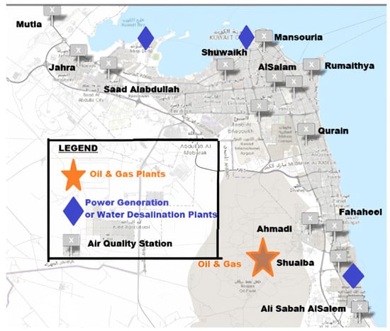
Figure 1.
Kuwait stations and plant map.
- The historic Shuwaikh Power Station in the capital region (North).
- The modern Saad Alabdullah facility serving the western districts (West).
- The industrial hub of Shuaiba (South).
- Critical urban monitoring points at Rumaithya and Road 50 Station.
- Suburban stations at Qurain and Mutla (West).
- Residential area monitors in Mansouria and Jahra (West).
- Industrial zone stations near Ahmadi and Fahaheel (South, near Oil and Gas facilities).
- Population centers at Al Salam (Center) and Ali Sabah Al Salem (South).
The dataset used in this research was provided by K-EPA and included data records captured at the 12 air quality stations between 1 January 2019 and 30 November 2021. Data from the K-EPA monitoring stations revealed that concentrations of PM2.5 frequently exceeded the thresholds for “Good” (0–12 g/m3) and “Moderate” (12.1–35.4 g/m3) categories, particularly in industrial and high-traffic areas such as Shuaiba, Ahmadi, and Road 50. In several instances, PM2.5 levels reached “Unhealthy for Sensitive Groups” (35.5–55.4 g/m3) or even “Unhealthy” (>55.5 g/m3) levels, especially during the summer and dust storm events. This gap between guideline values and observed data underscores the need for enhanced monitoring and mitigation strategies targeting fine particulate pollution in Kuwait.
4.1. Dataset Structure and Components
The dataset architecture incorporates 39 temporal, spatial, and environmental parameters (dataset columns), and AQI numbers, systematically organized to facilitate detailed analysis:
- Temporal and Spatial Parameters:
- –
- High-resolution timestamps for each measurement
- –
- Precise geographical locations of monitoring stations
- –
- Seasonal classification of data points
- Environmental Parameters: The dataset tracks multiple air quality indicators, measured with high precision:
- –
- Particulate Matter (PM10): Measured in micrograms per cubic meter (g/m3, also 24 h average and maximum).
- –
- Particulate Matter (PM2.5): Measured in micrograms per cubic meter (g/m3, also 24 h average and maximum).
- –
- Sulfur Dioxide (SO2): Measured in parts per billion (ppb, also 24 h average).
- –
- Hydrogen Sulfide (H2S): Measured in ppb.
- –
- Nitrogen Oxides (NO, NO2, NOx): Measured in ppb, also NOx 24 h average and NO2 1-hout average.
- –
- Ammonia (NH3): Measured in ppb.
- –
- Ozone (O3): Measured in ppb, also 8 h maximum.
- –
- Carbon Monoxide (CO): Measured in parts per million (ppm, also 8 h maximum).
- –
- Carbon Dioxide (CO2): Measured in ppm.
- –
- Wind Direction (WD) in degrees.
- –
- Wind Speed (WS) in m/s, also, 24 h average and maximum.
- –
- Temperature (TEMPERAT, degree Celsius), Relative Humidity (RH, percent).
- AQI Metrics: The dataset tracks multiple air quality indicators, measured with high precision:
- –
- PMI2.5_AQI.
- –
- PMI10_AQI.
- –
- SO2_AQI, NOX_AQI, NO2_AQI, CO_AQI, O3_AQI, Combined_AQI.
4.2. WHO and Environmental Agency Air Quality Standards: A Comprehensive Health Risk Assessment Framework
The World Health Organization (WHO) has established comprehensive guidelines for air quality assessment, particularly focusing on PM2.5 concentrations due to their significant health implications.
The PM2.5 Concentration Levels and Health Implications are:
- Optimal Air Quality (0–12 µg/m3): Air quality in this range represents ideal conditions with minimal health risks. The concentration of fine particulate matter is sufficiently low that both the general population and sensitive individuals can safely engage in outdoor activities without concern for respiratory impacts.
- Moderate Conditions (13–35 µg/m3): While generally safe for most individuals, these levels warrant awareness for sensitive populations. The air quality remains within acceptable parameters, though individuals with known sensitivities may need to monitor their exposure during extended outdoor activities.
- Sensitive Population Advisory (36–55 µg/m3): At this level, vulnerable populations require increased vigilance. This includes individuals with pre-existing respiratory conditions, those with cardiovascular sensitivities, young children and elderly populations, and pregnant women. The general population typically maintains normal resilience at these levels.
- Public Health Notice (56–150 µg/m3): These concentrations signal broader public health concerns, with potential impacts across all population segments. Sensitive groups face elevated risks, and the general public may begin experiencing mild respiratory symptoms or discomfort.
- Severe Health Alert (151–250 µg/m3): This range triggers public health warnings due to significant health risks. All population segments face an increased likelihood of adverse health effects, requiring protective measures and reduced outdoor exposure.
- Critical Health Emergency (251+ µg/m3): These extreme levels constitute a severe public health emergency, demanding immediate protective action for all population segments.
4.3. PM2.5 Air Quality Index (AQI) Standards and Pollutant Thresholds
The PM2.5 AQI uses a complex formula that changes between countries; for instance, the formula is different between the USA and China. In the dataset, the PM2.5 AQI is a continuous non-discrete real number, hence the ML models investigated in this work are regression models. Table 1 shows the mapping between the AQI categories, and the AQI levels and the various particle and gas quantities.

Table 1.
Air Quality Index (AQI) categories and associated pollutant ranges, adapted from [1].
The “24 h" Measurement Standards by Category are as follows:
- Good (AQI: 0–50): At this optimal level, air quality is ideal for all populations. The concentrations of pollutants are minimal, allowing for unrestricted outdoor activities and posing no health risks. These conditions represent the gold standard for urban air quality management.
- Moderate (AQI: 51–100): While still generally safe, these levels indicate a slight deterioration in air quality. Sensitive individuals might want to monitor their outdoor exposure, though the general population can continue normal activities without concern.
- Unhealthy Level 1 (AQI: 101–150): At this level, air quality begins to pose health risks to sensitive groups. People with respiratory conditions, the elderly, and young children should limit prolonged outdoor exposure. The general public might begin to notice mild respiratory discomfort.
- Unhealthy Level 2 (AQI: 151–200): These conditions represent a significant deterioration in air quality that affects all population groups. Outdoor activities should be limited, and sensitive groups should remain indoors whenever possible. Health effects may become more pronounced and widespread.
- Very Unhealthy (AQI: 201–300): This range signals a serious health risk for all populations. Emergency measures may be necessary, and all outdoor activities should be curtailed. Health effects can be immediate and severe, particularly for vulnerable populations.
- Hazardous (AQI: 301–500): These extreme levels constitute a health emergency. The entire population is at risk of experiencing serious health effects. Immediate action is required to protect public health, and authorities should consider implementing emergency measures such as closing schools and restricting outdoor activities.
4.4. Meteorological Parameters and Their Impact on Air Quality
The monitoring of meteorological conditions plays a crucial role in understanding and predicting air quality patterns. These parameters interact with pollutants in complex ways, significantly influencing their dispersion, concentration, and overall impact on air quality:
- Temperature (TEMPERAT °C): Temperature variations significantly influence air pollution dynamics through vertical air movement and pollutant dispersion, chemical reaction rates of atmospheric pollutants, formation of ground-level ozone in warmer conditions, thermal inversion effects that can trap pollutants, and the impact on local wind patterns and pollution transport.
- Relative Humidity (RH %RH): Humidity levels affect air quality through several mechanisms: particle size and composition modifications, formation of secondary aerosols, visibility reduction in high humidity conditions, impact on photochemical reaction rates, and the influence on pollutant deposition rates.
- Wind Speed (WS m/s): Wind speed is a critical factor in pollutant dispersion. Generally, higher speeds generally improve air quality through increased mixing. Low speeds can lead to pollutant accumulation. Noteworthy are the impact on dust suspension and transport, the influence on pollutant concentration patterns, and the effect on atmospheric stability conditions.
- Wind Direction (WD Deg): Wind direction determines the pollutant transport patterns from source regions, the impact areas of industrial emissions, the urban pollution distribution patterns, the regional air quality influences, and the seasonal pollution patterns based on prevailing winds.
These meteorological parameters work in concert to create unique atmospheric conditions that can either improve or deteriorate local air quality. Understanding these relationships is crucial for several key purposes. Accurate air quality classification enables authorities to predict and prepare for potential pollution events, while urban planning and development can be optimized to minimize adverse air quality impacts through thoughtful design and zoning. Industrial emission management benefits from this understanding by allowing facilities to adjust their operations based on atmospheric conditions, and public health protection measures can be implemented more effectively when the relationship between weather and air quality is well understood. Additionally, environmental policy development relies on comprehensive knowledge of these atmospheric interactions to create effective regulations that protect air quality while considering meteorological factors.
Next, we visually inspect and analyze the pruned air quality dataset.
5. Visual Analysis of PM2.5 Distribution and Environmental Correlations
After preparing the dataset and trimming it to 37,731 data rows, its content was thoroughly and visually analyzed. The scatter plots generated provide crucial insights into the spatial, temporal, and environmental factors affecting PM2.5 and PM10 Air Quality Index (AQI) levels across different geographical areas in Kuwait.
5.1. Environmental Feature Correlations with the AQI
As shown in Figure 2, the temperature impact analysis reveals that severe AQI levels (yellow bubbles) predominantly occur in the range of 15–45 °C, aligning with Kuwait’s typical temperatures and indicating pollution severity across different thermal conditions.
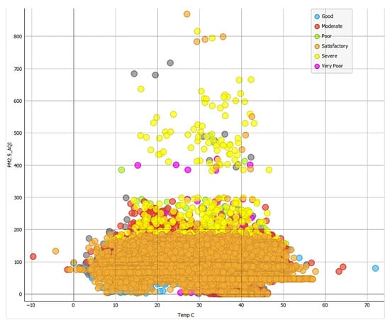
Figure 2.
Severe AQI level occurs mainly at temperatures in the range of 15–45 degrees Centigrade with a very few cases in the range of 80–100%.
Figure 3 demonstrates the humidity influence, where most severe pollution events occur at relative humidity below 50%, with rare cases in the range of 80–100% humidity. This pattern suggests that dry conditions may facilitate particulate matter accumulation, while higher humidity might assist in pollution suppression.
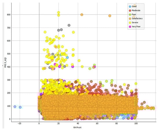
Figure 3.
Severe AQI happens mainly when RH % < 50%, with a very few cases in the range of 80–100% with a very few cases in the range of 80–100%.
5.2. Weather Patterns and Air Quality: Wind Conditions and Air Stagnation
Wind conditions play a crucial role in pollution patterns. As demonstrated in Figure 4, severe AQI is primarily observed at wind speeds below 12 m/s, where lower wind speeds may limit pollution dispersion and indicate that stagnant air conditions contribute to pollution accumulation. Figure 5 reveals that the highest pollution levels occur with wind direction in the range of 240–340 degrees, suggesting that wind patterns influence pollutant transport from industrial areas.
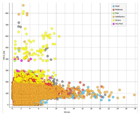
Figure 4.
Severe AQI level happens mainly when wind speed < 12 m/s with a very few cases in the range of 80–100%.
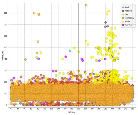
Figure 5.
Severe AQI level happens mainly when wind direction is in the range of 240–340 degrees with a very few cases in the range of 80–100%.
This observation aligns with the phenomenon of air stagnation, which, as defined by the Spokane Regional Clean Air Agency [27], occurs when air becomes trapped in a region with minimal movement, typically caused by high-pressure systems that inhibit vertical motion and air dispersal. During these stagnation events, the lack of airflow leads to the accumulation of pollutants in the atmosphere. Our analysis of Kuwait’s air quality data confirms this relationship between air stagnation and pollution levels, particularly in industrial areas such as Fahaheel and Mutla. The combination of low wind speeds and specific wind directions creates conditions conducive to pollutant accumulation, especially when winds blow from industrial zones (240–340 degrees). These findings demonstrate how meteorological conditions, particularly wind patterns, interact with industrial emissions to influence local air quality levels.
5.3. Temporal and Seasonal Patterns
Figure 6 demonstrates a strong correlation between PM2.5_AQI and 24 h average measurements, validating measurement consistency over daily periods. The seasonal distribution analysis in Figure 7 and Figure 8 reveals that severe AQI events predominantly occur in summer and spring, with the highest PM2.5_AQI levels recorded during these seasons. This pattern correlates with increased dust storms and atmospheric stability, and may reflect seasonal variations in industrial activity.
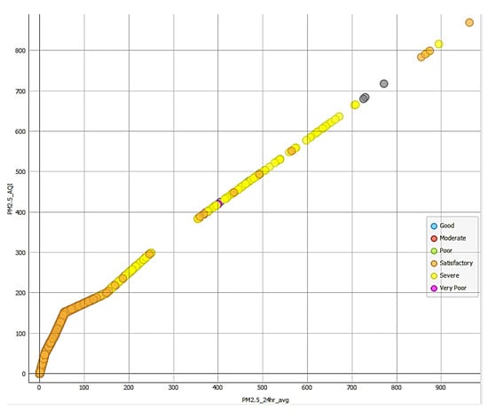
Figure 6.
Strong relationship between PM2.5_AQI and PM2.5_24hr_avg degrees with a very few cases in the range of 80–100%.
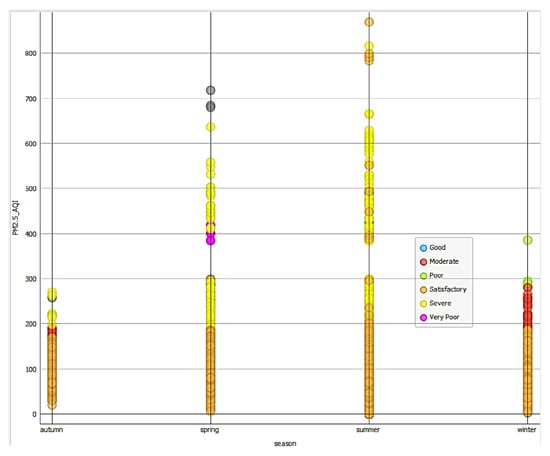
Figure 7.
Severe AQI happens mainly in summer and spring degrees with a very few cases in the range of 80–100%.

Figure 8.
Highest PM2.5_AQI occur in summer and spring seasons degrees with a very few cases in the range of 80–100%.
5.4. Insights from Visual Analysis: Implications for Model Optimization and Environmental Management
The visualization analysis reveals complex relationships between pollution levels, geographical location, and environmental conditions in Kuwait. The addition of severity level analysis and PM2.5/PM10 correlations provides deeper insights into pollution patterns and their spatial distribution. Industrial areas (e.g., Fahaheel, Mutla, Ahmadi) show consistently higher pollution levels, with environmental factors such as temperature, humidity, and wind patterns playing crucial roles in pollution dispersion and accumulation.
These insights are valuable for feature selection of the dataset used by the machine learning models and to ultimately help in developing targeted air quality management strategies and public health protection measures, particularly in high-risk areas identified through the spatial analysis. This data-driven approach to parameter tuning, informed by detailed environmental pattern analysis, enhances the ML models’ ability to capture complex air quality dynamics and provide more accurate classifications for different geographical locations and environmental conditions.
5.5. Industrial Proximity and Environmental Drivers of Air Quality in Kuwaiti Regions: A Multivariate Visual Analysis
5.5.1. Industrial Impact on Regional Air Quality
Mutla and Ahmadi, both located close to oil and gas facilities or other industrial plants, exhibit the worst Air Quality Index (AQI) values among the studied locations, as shown in Figure 9. This suggests that proximity to industrial activities significantly contributes to poor air quality in these areas, with AQIs consistently higher compared to other locations. Figure 10 highlights that Mutla experienced a wide range of combined AQI values, indicating significant variability in air quality over time. In contrast, Ahmadi and Fahaheel, which are also near oil facilities, showed narrower ranges of combined AQI. This suggests that, while all three locations are affected by industrial activities, although Mutla is far from the oil fields and refineries, its poor air quality is likely influenced by its proximity to other industrial plants.
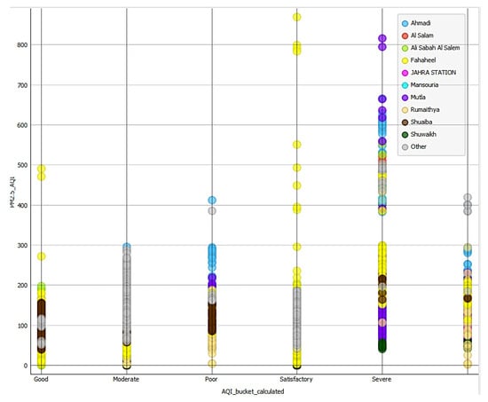
Figure 9.
Mutla and Ahmadi (close to oil and gas facilities or other plants) have the worst AQIs degrees with a very few cases in the range of 80–100%.
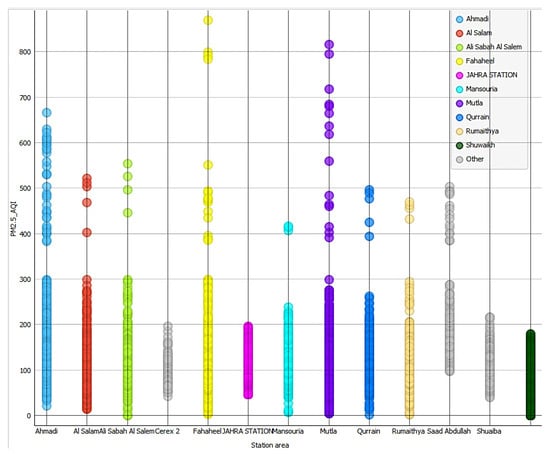
Figure 10.
Mutla experienced a wide range of combine-AQI, compared to Ahmadi and Fahaheel (all near oil) which experienced narrower ranges of combined_AQI degrees with a very few cases in the range of 80–100%.
5.5.2. PM2.5 Concentration and Temperature Effects
Figure 2 shows that temperatures associated with severe and very poor AQI conditions range between 15 °C and 45 °C. This wide temperature range suggests that poor air quality is not limited to a specific season but can occur across varying climatic conditions. Higher temperatures, however, may exacerbate pollution levels due to increased photochemical reactions and stagnation of air.
5.5.3. Wind Patterns and Air Quality Correlation
Figure 4 indicates that the worst wind speeds associated with poor air quality range from 1 to 11 m per second (m/s). Lower wind speeds (closer to 1 m/s) are often linked to poor air quality because they reduce the dispersion of pollutants, allowing them to accumulate in the atmosphere. Higher wind speeds (up to 11 m/s) may also contribute to poor air quality by transporting pollutants from nearby industrial sources. Furthermore, the worst wind directions associated with poor air quality are between 240 and 340 degrees. This suggests that pollutants are being carried from specific directions, likely corresponding to the locations of industrial facilities or other pollution sources. Understanding wind direction is crucial for identifying the sources of air pollution and implementing targeted mitigation measures.
5.5.4. PM2.5 Temporal Analysis and Seasonal Variations
As shown in Figure 6, there is a very strong correlation between PM2.5_24hr_avg (the 24 h average concentration of PM2.5) and PM2.5_AQI. This indicates that PM2.5 levels are a dominant factor in determining the overall AQI in these regions. The strong correlation underscores the importance of monitoring and controlling PM2.5 emissions to improve air quality. The worst seasons for air quality are summer, followed by spring. During summer, higher temperatures and increased solar radiation can enhance the formation of secondary pollutants like ozone and particulate matter. Spring may also experience poor air quality due to dust storms or other seasonal factors. These seasonal trends highlight the need for targeted air quality management strategies during these periods.
5.5.5. Critical Air Pollutants Contributing to Severe Air Quality Degradation
Finally, the analysis of air pollutants reveals that carbon dioxide (CO2), carbon monoxide (CO), and hydrogen sulfide (H2S) are the primary contributors to severe and very poor air quality conditions in Kuwait, as shown in Figure 11, indicating the presence of incomplete combustion processes from both industrial sources and vehicle emissions.
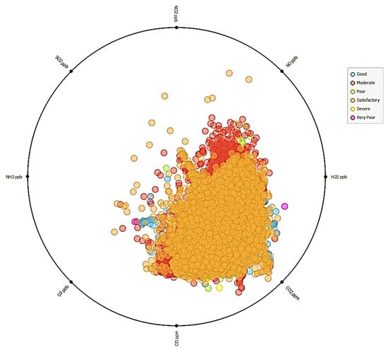
Figure 11.
Worst air polluters (severe and very poor) are CO2 ppm, CO ppm, and H2S ppb with a very few cases in the range of 80–100%.
Hydrogen sulfide (H2S), measured in parts per billion (ppb), emerges as another critical pollutant, particularly in areas near oil and gas facilities.
5.6. Correlations and Other Statistics
As a result of further data analysis, the mean and maximum values for each of the air quality stations are presented in Table 2.
Table 2.
Summary of air quality data by station.
Our analysis of Figure 2, Figure 3, Figure 4, Figure 5, Figure 6, Figure 7, Figure 8, Figure 9, Figure 10 and Figure 11 reveals significant correlations between various air quality parameters, with particular emphasis on the relationships between PM2.5, PM10, and other pollutants. The following features correlated best with the PM2.5 AQI target:
- Correlation of +0.916 with PM2.5_24hr_avg.
- Correlation of +0.634 with PM2.5_24hr_max.
- Correlation of +0.489 with PM2.5 g/m3(L).
- Correlation of +0.410 with PM10_24hr_avg.
- Correlation of +0.380 with Combined_AQI.
Note that none of the gases correlated significantly with the PM2.5 target. We will use these results in guiding the feature selection experiments in Section 6.
5.7. Implications for Feature Selection and Model Development
By referencing the above figures, the analysis provides a comprehensive understanding of the factors contributing to poor air quality in the studied regions, including industrial proximity, meteorological conditions, and seasonal variations. These insights will guide the selection of features in the five ML experiments, which will be presented in the next section. As one desired objective is to reduce the number of features to a minimum and keep those most relevant that impact air quality, and in order to reduce the long ML model training times, this analysis will help identify the key variables to keep in the ML models. Notably, increased PM2.5 concentrations associated with higher wind speeds often suggest the influence of long range transport rather than local emission sources [12].
Next, we discuss the optimal ML model parameters, the five experiments with various feature selections, and present the associated ML performance metrics.
6. ML Parameter Optimization and Experimental Results
Through an iterative trial-and-error process of optimization, we refined specific parameters for each ML model to achieve optimal performance, reflected by metrics such as the MSE and . These refined parameters are presented in Table 3. These optimal parameters were used in our five experiments.
Table 3.
Optimal ML model parameters for classifying the PM2.5_AQI.
Our research focused on developing ML regression models for the PM2.5 Air Quality Index (AQI) levels utilizing a refined dataset of 37,731 instances. In our five experiments, using a random sampling approach, we adopted random sampling with 66% of the data (24,902 instances or rows) randomly allocated for training and 34% (12,829 instances) for testing.
6.1. Experiment 1: With All the Original Dataset Features
Experiment 1 kept all the original dataset features. As shown in Table 4, Gradient Boosting and AdaBoost demonstrated exceptional performance, with nearly perfect R2 values of 0.999 and remarkably low error metrics. The Decision Tree classifier also showed excellent results with very low error metrics (MSE = 3.526, RMSE = 1.878, MAE = 0.116) and a high R2 value of 0.998, indicating highly accurate predictions. Random Forest achieved good results with moderate error metrics (MSE = 116.603, RMSE = 10.798, MAE = 6.935) and a strong R2 value of 0.936, suggesting effective modeling of the target variable. Linear Regression showed mediocre performance with relatively high error metrics (MSE = 773.726, RMSE = 27.816, MAE = 21.515) and a moderate R2 value of 0.574, indicating limited ability to capture non-linear relationships in the data. SVMs, neural networks, and kNN exhibited poor performance.
Table 4.
Performance of the eight machine learning algorithms for experiment 1.
Boosting and AdaBoost emerged as the most effective models for PM2.5_AQI prediction, followed closely by the Decision Tree classifier. These models demonstrated superior ability to capture complex patterns in the data while maintaining excellent generalization capabilities. However, the used dataset contained a large number of features which elongate the training time of the ML models. In the next experiments, we seek to prune features while achieving good performance metrics to reduce the ML model training times.
6.2. Experiment 2: Refined Model Analysis with Key Features
After deleting (unselecting as features) all features (refer to Section 4.1) except: date and time, station, all the chemical substances (CO, H2S…) and their AQI metrics, temperature, RH, WS, WD, and season, we retrained the eight ML models and obtained the results presented in Table 5. The justification for omitting the gases were their low correlation with the target as discussed in Section 5.6. Because the correlations of the AQI numbers with the target were obvious, we also omitted the AQI features. In this experiment, AdaBoost, Decision Tree, and Gradient Boosting classifiers maintained their superior performance even with the reduced feature set. The MSEs rose and the R2 s dropped considerably compared to the experiments, given that average and maximum values of PM2.5, PM10, and chemicals were skipped.
Table 5.
Performance of the eight machine learning algorithms for experiment 2.
Neural networks and SVMs performed poorly. The superior performance of AdaBoost, Decision Tree, and Gradient Boosting suggests that these algorithms are particularly well-suited for handling the non-linear relationships and complex interactions present in air quality data, even when 24 h average and maximum data are removed.
6.3. Experiment 3: Advanced Model Evaluation with Aggressive Pruning
In experiment 3, after skipping all other features, we retained only key environmental parameters: Temperature (Temp), Relative Humidity Percentage (RH Prcnt), Wind Speed (WS), Wind Direction (WD), PM2.5 24 h average (PM2.5_24hr_avg), PM2.5 24 h maximum (PM2.5_24hr_max), and season. In this experiment, we retained the PM2.5-related features as they correlated well with the PM2.5 AQI target, and sought to assess the impact of the environmental features. As detailed in Table 6, three machine learning algorithms demonstrated exceptional performance with the optimized feature set: AdaBoost, Gradient Boosting, and Decision Tree. Linear Regression and Support Vector Machine (SVM) were the worst performers.
Table 6.
Performance of the eight machine learning algorithms for experiment 3.
6.4. Experiment 4: Model Performance Under Challenging Data Conditions
In this experiment with a minimal feature set, retaining only: PM10 (g/m3 L), NOX (ppb), temperature, wind speed (WS m/s), and PM2.5 (g/m3). This significantly reduced feature set resulted in notably degraded performance across all models, as detailed in Table 7. Random Forest emerged as the strongest performer, though with notably lower accuracy than in previous experiments. This experiment revealed important insights about model performance under limited feature conditions:
Table 7.
Performance of the eight machine learning algorithms for experiment 4.
- The significantly reduced feature set led to poor performance across all models.
- Random Forest’s relative superiority suggests better resilience to limited features.
- The generally lower performance across all models indicates the importance of the feature selection.
Keeping PM2.5 (g/m3) as the only PM2.5-related feature led to a severe degradation in the performance metrics, given its low Pearson-R correlation with the target.
6.5. Experiment 5: Final Model Evaluation with Optimized Features
In this experiment with only five features, we retained two features which correlated well with the target: PM2.5 24 h average (PM2.5_24hr_avg), PM10 (g/m3L), along with NOX (ppb), temperature, and wind speed (WS m/s). All other features were deleted. Table 8 demonstrates exceptional performance from ensemble methods: Gradient Boosting and AdaBoost achieved perfect predictions, while Decision Tree maintained outstanding performance, all with only five features.
Table 8.
Performance of the eight machine learning algorithms for experiment 5 showing the superior performance of Gradient Boosting and AdaBoost algorithms.
This final experiment provides decisive evidence that ensemble methods, particularly Gradient Boosting and AdaBoost, are optimal for PM2.5 prediction tasks. The perfect R2 scores and minimal error metrics demonstrate their superior ability to capture complex environmental relationships, handle varying data patterns, maintain prediction accuracy, and adapt to optimized feature sets.
In the next section, we analyze our experimental results.
7. Research Result Analysis
- The strong correlation between PM2.5 and PM10 is partially explained by the inherent inclusion of PM2.5 particles within PM10 measurements. Given the high temperatures and relative humidity in Kuwait, atmospheric chemical reactions accelerate and generate secondary PM. This explains why the ML regression models in experiments with PM2.5-related and PM10-related features performed better than other experiments which did not contain them.
- The weak correlations of the gases features with the PM2.5 AQI target explain why the experiment 2 performance metrics were not strong, while the experiment 5 metrics were better.
- (a)
- (b)
- The superiority of Gradient Boosting, AdaBoost, and Tree in classifying the air quality data, as the data fits the simple tree patterns of these ML models. Ensembles of weak decision tree models, namely Gradient Boosting and AdaBoost, fall into the general ML group of Decision Trees.
- (c)
- Pruning the features with careful feature selection enhanced the performance of Gradient Boosting, AdaBoost, and Tree, in particular the MSEs of experiment 5 (with only five features) which were lower than in experiment 1.
- (d)
- The good performances obtained in experiments 1, 3, and 5 are attributed to mainly the presence of PM2.5 and PM10 features which correlate well with PM2.5_AQI. However, experiment 4 reveals poor performance results by the eight ML models although PM2.5 g/m3L was part of the selected features, as the PM2.5 g/m3L feature’s Pearson-R correlation factor with the target was only 0.489.
- (e)
- Comparing the selected features of experiments 4 (where the ML models performed poorly) and 5 (where the ML models performed well), experiment 5 added PM2.5_24-h_average as feature (refer to Figure 5) which was critical in boosting the performance. Although the PM2.5 g/m3L readings and weather factors such as WS and temperature were important, given that we trimmed the dataset to only 13.4% of its original size, the 24 h average of the PM2.5 g/m3L samples was crucial in compensating for the aggressive pruning of data instances (rows).
- (f)
- Deep learning models such as LSTM were not needed, given the goodness of the obtained results.
In order to visualize the good performance of the Tree-based ML models, Figure 12, Figure 13 and Figure 14 display the time series plots of PM2.5 AQI, Gradient Boosting (one of the three Tree-based ML models), and SVM, all versus date and time. The legends in Figure 12, Figure 13 and Figure 14 represent the ranges of the actual PMI2.5 AQI values in color. Figure 12 displays the actual PM2.5 AQI data which is the target of the ML models. Figure 13 displays one good performing ML model, Gradient Boosting, where the legend represent the actual PMI2.5 AQI levels for comparison and indicating good matching between the actual data and the ML classification. Figure 14 illustrates how an underperforming ML model, SVM, performs in comparison.
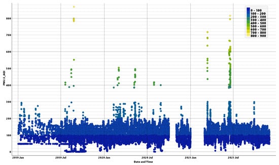
Figure 12.
PMI2.5 AQI numbers vs. date plot (legend represents the actual PM2.5 AQI data).
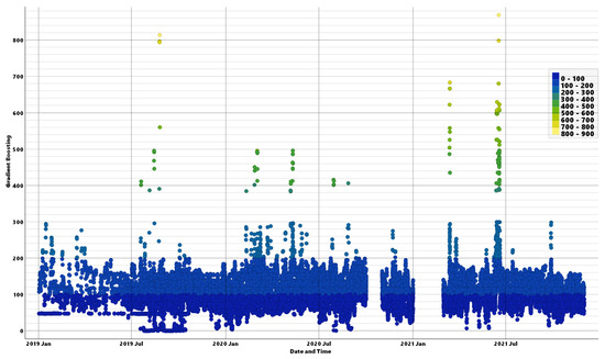
Figure 13.
PM2.5 AQI numbers vs. date and time plot.
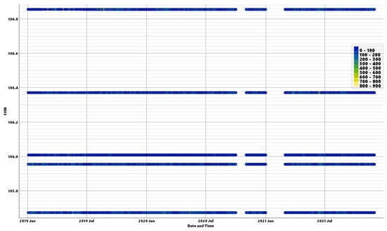
Figure 14.
SVM-produced PM2.5 AQI numbers vs. date and time plot.
8. Supporting the Formulation of Public Policies
As shown by Table 1, the mean PM2.5 AQI is at unhealthy or worse levels at several locations in Kuwait. The maximum 24 h PM2.5 levels are also alarming. As a result, we draw some public policies recommendations aimed at improving environmental sustainability and reducing air pollution. These policy recommendations will focus on reducing industrial emissions, transitioning to cleaner energy sources, and promoting sustainable transportation solutions. Below is an expanded discussion of key policies.
8.1. Reducing Industrial Gas Flaring
Policy Objective: Minimize gas flaring from oil and gas operations to reduce air pollution and greenhouse gas emissions.
Discussion: As shown in Table 1, various locations near oil and gas plants demonstrate worse (mean and maximum PM2.5) air quality levels; for instance, Fahaheel, Ahmadi, and Shuaiba. Gas flaring releases particulate matter (PM2.5) and various gases contributing significantly to air pollution and climate change. Kuwait’s heavy reliance on fossil fuel extraction results in large-scale flaring, particularly in oil refineries and petrochemical plants. Relevant policies should focus on implementing stricter regulations and industry-specific limits on flaring volumes, requiring companies to adhere to international best practices. The establishment of tax incentives or subsidies for oil companies investing in gas recovery and utilization technologies would serve as a crucial incentive for flare gas recovery. Additionally, promoting flare gas-to-energy projects would enable the conversion of captured gas into electricity, creating value from what would otherwise be wasted. To ensure compliance, authorities should mandate real-time emissions monitoring through satellite-based tracking and AI-powered analytics, while also introducing public reporting requirements for emissions data. The proposed measures would result in reductions in PM2.5 levels leading to improved air quality, helping Kuwait align with its climate commitments and international environmental obligations. Furthermore, the economic advantages of utilizing previously wasted gas for energy production would create new revenue streams while promoting resource efficiency.
8.2. Transitioning Away from Hydrocarbon-Based Electricity Generation
Policy Objective: Reduce Kuwait’s dependence on fossil fuels for electricity generation by accelerating the adoption of renewable energy.
Discussion: As shown in Table 1, various locations near electricity generating plants demonstrate worse (mean and maximum PM2.5) air quality levels; for instance, Mutla and Saad Alabdulla. Power plants burning natural gas and oil are among the largest contributors to air pollution and carbon emissions in Kuwait. Kuwait’s high electricity demand, especially during summer, leads to an increased burning of hydrocarbons, worsening air quality. It is recommended that Kuwait should establish renewable energy targets for its electricity grid, aiming for 30% of total energy from renewables by 2035, instead of the 15% goal of the Kuwait 2035 vision. This would be supported by fast-tracking solar and wind energy projects through public–private partnerships, while providing incentives for households and businesses to install rooftop solar panels, complemented by net metering policies allowing excess energy to be sold back to the grid. The decarbonization of power plants would involve gradually retiring older, inefficient fossil-fuel-based facilities and replacing them with cleaner alternatives, while encouraging the adoption of carbon capture and storage technology at existing plants. Grid modernization efforts would focus on investing in smart grid technology to optimize electricity distribution and balance demand with renewable energy supply, alongside expanding large-scale battery storage solutions to store excess solar and wind energy for use during peak demand periods.
The implementation of clean energy initiatives would yield decreased air pollution from power generation and consequently, better public health outcomes for the population.
8.3. Expanding Adoption of Electric Vehicles (EVs)
Policy Objective: Accelerate the transition from gasoline and diesel vehicles to electric vehicles (EVs) to lower transportation-related emissions.
Discussion: As supported by the findings in [1], the transportation sector is a major contributor to PM2.5, NOx, and CO2 emissions. Kuwait has one of the highest car ownership rates per capita, leading to high traffic congestion and air pollution.
To promote electric vehicle adoption, a comprehensive approach to incentives and infrastructure development is essential. The strategy should begin with introducing financial incentives such as tax breaks and purchase subsidies to make EVs more affordable, along with providing free or discounted registration fees for EV owners. The development of charging infrastructure would focus on expanding public EV charging networks across cities, highways, and residential areas, while requiring new building projects to include EV charging stations in their design. The transition to electric vehicles would bring a significant reduction in urban air pollution that would lead to better respiratory health for residents. The widespread adoption of EVs would result in lower greenhouse gas emissions, supporting Kuwait’s climate goals and environmental commitments.
8.4. Continue Electricity Imports from Neighboring Countries
Policy Objective: Ensure energy reliability while reducing domestic hydrocarbon consumption by continuing to import electricity from cleaner regional sources.
Discussion: Kuwait’s electricity demand peaks during the summer, leading to an over-reliance on oil and gas power plants, which exacerbate air pollution. Power blackouts during peak power consumption periods have been common in the past two years in Kuwait. Neighboring countries (e.g., Saudi Arabia, UAE) are investing in large-scale renewable energy projects, creating an opportunity for cleaner electricity imports. The implementation of regional power integration would provide immediate benefits through the reduction in air pollution by lowering local fossil fuel combustion.
9. Conclusions and Future Research
This research advances the understanding of air pollution prediction through a comprehensive analysis of multiple pollutants and meteorological parameters in Kuwait’s unique environmental context. Our thorough data visualization and analysis and systematic evaluation of eight machine learning algorithms provides valuable insights for both environmental monitoring and public health protection. Our research study revealed that Tree-based ML models, particularly Gradient Boosting and AdaBoost, demonstrate superior performance in predicting air quality indices as demonstrated by low MSE values below 1.5 and values of 0.999 or above. Through five distinct experiments, we identified optimal feature sets and model parameters that significantly enhance prediction accuracy. Given the aggressive pruning, it was revealed that keeping the 24 h PM2.5 average as feature (and/or other PM-related features) was crucial in boosting the performance of the ML models, as revealed by experiment 5.
The findings from this research have practical applications for environmental management and public health protection. The ability to predict severe air quality events enables proactive measures to protect vulnerable populations. Our improved understanding of pollution patterns in industrial areas facilitates more effective emission control strategies and urban planning decisions. The development of more targeted air quality management strategies, informed by our model predictions, can lead to more efficient resource allocation for environmental protection.
Our approach to feature selection optimization through correlation analysis has proven highly effective in enhancing model performance. The integration of temporal and spatial factors in prediction models provides a more comprehensive understanding of pollution dynamics. While the results of this study are promising, several important areas warrant further investigation. The long-term performance of these models under varying environmental conditions needs to be evaluated to ensure their reliability across different scenarios. Future research should focus on integrating real-time data for immediate classification and prediction capabilities, which would enhance the practical utility of these models in environmental monitoring systems. The expansion of this modeling approach to other geographical contexts would help validate its broader applicability and identify region-specific adaptations that might be necessary. Additionally, investigating additional feature combinations could potentially uncover new patterns and relationships in air quality dynamics.
Author Contributions
The study was conceptualized by H.A. and F.N.S. Methodological design, software development, and model implementation were jointly carried out by H.A. and F.N.S. A.A. (Ahmad Alsaber) provided the primary dataset, while M.A. contributed to the validation and verification of environmental data quality based on his domain expertise. Formal analysis was conducted by H.A. The original draft of the manuscript was prepared by H.A. and F.N.S., with A.A. (Abdullah Abonamah) providing critical review, revision, and editorial input. Visualization was performed by F.N.S. Supervision, project administration, and funding acquisition were led by H.A. All authors have read and agreed to the published version of the manuscript.
Funding
This research was funded by the Kuwait Foundation for the Advancement of Sciences (KFAS), under project code PN23-19TM-1859.
Institutional Review Board Statement
Not applicable.
Informed Consent Statement
Not applicable.
Data Availability Statement
The data that support the findings of this study are available from the corresponding author upon reasonable request. Derived datasets and analysis scripts can also be shared for academic and research purposes.
Acknowledgments
The authors gratefully acknowledge that this project was funded by the Kuwait Foundation for the Advancement of Sciences (KFAS) under project code PN23-19TM-1859. The authors also thank the Kuwait College of Science and Technology (KCST) for supporting this research.
Conflicts of Interest
The authors declare no conflict of interest. The funders had no role in the design of the study; in the collection, analyses, or interpretation of data; in the writing of the manuscript; or in the decision to publish the results.
References
- Alsaber, A.; Alsahli, R.; Al-Sultan, A.; Abu Doush, I.; Sultan, K.; Alkandary, D.; Coffie, E.; Setiya, P. Evaluation of various machine learning prediction methods for particulate matter PM 10 in Kuwait. Int. J. Inf. Technol. 2023, 15, 4505–4519. [Google Scholar]
- Alrashidi, H.; Almujally, N.; Kadhum, M.; Ullmann, T.D.; Joy, M. Evaluating an Automated Analysis Using Machine Learning and Natural Language Processing Approaches to Classify Computer Science Students’ Reflective Writing. In Pervasive Computing and Social Networking; Ranganathan, G., Bestak, R., Fernando, X., Eds.; Lecture Notes in Networks and Systems; Springer: Singapore, 2022; Volume 475, pp. 425–437. [Google Scholar] [CrossRef]
- Marjovi, A.; Arfire, A.; Martinoli, A. High resolution air pollution maps in urban environments using mobile sensor networks. In Proceedings of the 2015 International Conference on Distributed Computing in Sensor Systems, Fortaleza, Brazil, 10–12 June 2015; pp. 11–20. [Google Scholar]
- Zhao, J.; Ghedira, H.; Temimi, M. Detection of oil pollution in the arabian gulf using optical remote sensing imagery. In Proceedings of the 2014 IEEE Geoscience and Remote Sensing Symposium, Quebec City, QC, Canada, 13–18 July 2014; pp. 1453–1456. [Google Scholar]
- Mohamed Al-Damkhi, A.; Ahmed Abdul-Wahab, S.; Mansour Al-Khulaifi, N. Kuwait’s 1991 environmental tragedy: Lessons learned. Disaster Prev. Manag. Int. J. 2009, 18, 233–248. [Google Scholar] [CrossRef]
- Dairi, A.; Harrou, F.; Khadraoui, S.; Sun, Y. Integrated multiple directed attention-based deep learning for improved air pollution forecasting. IEEE Trans. Instrum. Meas. 2021, 70, 1–15. [Google Scholar] [CrossRef]
- Du, S.; Li, T.; Yang, Y.; Horng, S.J. Deep air quality forecasting using hybrid deep learning framework. IEEE Trans. Knowl. Data Eng. 2019, 33, 2412–2424. [Google Scholar] [CrossRef]
- Liang, Y.C.; Maimury, Y.; Chen, A.H.L.; Juarez, J.R.C. Machine learning-based prediction of air quality. Appl. Sci. 2020, 10, 9151. [Google Scholar] [CrossRef]
- Li, S.; Xie, G.; Ren, J.; Guo, L.; Yang, Y.; Xu, X. Urban PM2.5 concentration prediction via attention-based CNN–LSTM. Appl. Sci. 2020, 10, 1953. [Google Scholar] [CrossRef]
- Zhang, Z.; Zhang, S.; Zhao, X.; Chen, L.; Yao, J. Temporal difference-based graph transformer networks for air quality PM2.5 prediction: A case study in China. Front. Environ. Sci. 2022, 10, 924986. [Google Scholar] [CrossRef]
- Wang, X.; Shi, G.; Huang, C.; Wang, M.; Wang, Z. Affect of Power Consumption Decline of Air Compressor on Oil Saving of Heavy-duty Vehicle. In Proceedings of the 2013 IEEE Vehicle Power and Propulsion Conference (VPPC), Beijing, China, 15–18 October 2013; pp. 1–5. [Google Scholar]
- Chen, Z.Y.; Zhang, T.H.; Zhang, R.; Zhu, Z.M.; Yang, J.; Chen, P.Y.; Ou, C.Q.; Guo, Y. Extreme gradient boosting model to estimate PM2.5 concentrations with missing-filled satellite data in China. Atmos. Environ. 2019, 202, 180–189. [Google Scholar] [CrossRef]
- Liu, H.; Wu, H.; Lv, X.; Ren, Z.; Liu, M.; Li, Y.; Shi, H. An intelligent hybrid model for air pollutant concentrations forecasting: Case of Beijing in China. Sustain. Cities Soc. 2019, 47, 101471. [Google Scholar] [CrossRef]
- Lyu, Y.; Ju, Q.; Lv, F.; Feng, J.; Pang, X.; Li, X. Spatiotemporal variations of air pollutants and ozone prediction using machine learning algorithms in the Beijing-Tianjin-Hebei region from 2014 to 2021. Environ. Pollut. 2022, 306, 119420. [Google Scholar] [CrossRef] [PubMed]
- Islam, A.R.M.T.; Al Awadh, M.; Mallick, J.; Pal, S.C.; Chakraborty, R.; Fattah, M.A.; Ghose, B.; Kakoli, M.K.A.; Islam, M.A.; Naqvi, H.R.; et al. Estimating ground-level PM2.5 using subset regression model and machine learning algorithms in Asian megacity, Dhaka, Bangladesh. Air Qual. Atmos. Health 2023, 16, 1117–1139. [Google Scholar] [CrossRef] [PubMed]
- Aram, S.; Nketiah, E.; Saalidong, B.; Wang, H.; Afitiri, A.R.; Akoto, A.; Lartey, P. Machine learning-based prediction of air quality index and air quality grade: A comparative analysis. Int. J. Environ. Sci. Technol. 2024, 21, 1345–1360. [Google Scholar] [CrossRef]
- MachineLearning.org.in. Accuracy, Precision, Recall, and F1-Score. 2024. Available online: https://machinelearning.org.in/accuracy-precision-recall-and-f1-score/ (accessed on 18 May 2025).
- Canbek, O.; Szeto, C.; Washburn, N.R.; Kurtis, K.E. A quantitative approach to determining sulfate balance for LC3. Cement 2023, 12, 100063. [Google Scholar] [CrossRef]
- Bellinger, C.; Jabbar, M.; Zäıane, O.; Osornio-Vargas, A. A systematic review of data mining and machine learning for air pollution epidemiology. BMC Public Health 2017, 17, 907. [Google Scholar] [CrossRef] [PubMed]
- Zhang, B.; Duan, M.; Sun, Y.; Lyu, Y.; Hou, Y.; Tan, T. Air quality index prediction in six major chinese urban agglomerations: A comparative study of single machine learning model, ensemble model, and hybrid model. Atmosphere 2023, 14, 1478. [Google Scholar] [CrossRef]
- Morapedi, T.; Obagbuwa, I. Air pollution particulate matter (pm2.5) prediction in south african cities using machine learning techniques. Front. Artif. Intell. 2023, 6, 1230087. [Google Scholar] [CrossRef] [PubMed]
- Pant, A.; Sharma, S.; Pant, K. Evaluation of machine learning algorithms for air quality index (aqi) prediction. J. Reliab. Stat. Stud. 2023, 16, 229–242. [Google Scholar] [CrossRef]
- Castelli, M.; Clemente, F.; Popovič, A.; Silva, S.; Vanneschi, L. A machine learning approach to predict air quality in california. Complexity 2020, 2020, 8049504. [Google Scholar] [CrossRef]
- Nandi, A.; Kaur, N.; Singla, P. Simple augmentations of logical rules for neuro-symbolic knowledge graph completion. In Proceedings of the 61st Annual Meeting of the Association for Computational Linguistics, Toronto, ON, Canada, 9–14 July 2023. [Google Scholar]
- Tasioulis, T.; Karatzas, K. Reviewing explainable artificial intelligence towards better air quality modelling. In Environmental Informatics; Springer: Berlin/Heidelberg, Germany, 2023; pp. 3–19. [Google Scholar]
- Demšar, J.; Curk, T.; Erjavec, A.; Gorup, Č.; Hočevar, T.; Milutinovič, M.; Možina, M.; Polajnar, M.; Toplak, M.; Starič, A.; et al. Orange: Data mining toolbox in Python. J. Mach. Learn. Res. 2013, 14, 2349–2353. [Google Scholar]
- Văduva, A.G.; Munteanu, M.; Oprea, S.V.; Bâra, A.; Niculae, A.M. Understanding climate change and air quality over the last decade: Evidence from news and weather data processing. IEEE Access 2023, 11, 144631–144648. [Google Scholar] [CrossRef]
Disclaimer/Publisher’s Note: The statements, opinions and data contained in all publications are solely those of the individual author(s) and contributor(s) and not of MDPI and/or the editor(s). MDPI and/or the editor(s) disclaim responsibility for any injury to people or property resulting from any ideas, methods, instructions or products referred to in the content. |
© 2025 by the authors. Licensee MDPI, Basel, Switzerland. This article is an open access article distributed under the terms and conditions of the Creative Commons Attribution (CC BY) license (https://creativecommons.org/licenses/by/4.0/).