Evaluating Middle-Distance Passenger Transportation: A Comparison of the Time Efficiency, Sustainability, and Break-Even Distances Between High-Speed-Rail and Air Travel in Sweden

Abstract

Debate regarding the use of airplanes or high-speed trains in middle-distance passenger transportation has evolved into a strong field of research. With the aim to mitigate the environmental footprint of air travel, the European Union’s initiatives are focused on redirecting passengers from airplanes to high-speed trains. This shift is hampered by significant variations in train accessibility across Europe. Using Sweden as an example, we tested the break-even distance and evaluated the findings from both a time-efficiency perspective and a sustainability perspective. Airplanes hold the upper hand on high-speed trains in middle-distance passenger transportation from the time perspective. This perspective provides us with a clear answer, but if we consider the sustainability perspective, it may affect the results. The results indicate that the presented proof of concept makes sense and can be easily adapted to any decision-making process regarding the choice of the preferable transportation mode, although the procedure is extremely time consuming. For policymakers, this proof of concept can represent a priceless tool because the resulting figures carry valuable information about (under)developed and (less-)integrated transportation modes in commuting and transportation systems.

1. Introduction

The development of transportation infrastructure caused rapid mobility growth, so tendencies toward sustainable transportation have emphasized the need for a change in mobility. The European Union aims to shift passenger traffic at middle distances from airplanes to railways, specifically, to high-speed rail (HSR). Redirecting passengers from airplanes to high-speed trains would reduce the negative environmental impacts of air travel. Transporting passengers by train results in 80% less CO₂ emission than air travel and 75% less CO₂ emission than road transportation [1,2,3]. Straus et al. [4], based on an analysis of 2000 routes across China, report that airplanes emit up to seven times more CO₂ compared to high-speed trains, highlighting the significant environmental advantage of HSR over air travel. Currently, HSR carries significantly fewer passengers than air travel. In 2019, the share of passenger transportation by HSR at middle distances (e.g., between 500 and 1000 km) was only 13% [2,3]. Other studies have shown that for distances between 200 km and 1000 km, HSR is already competitive with air travel [5,6,7].

There are many comparisons between different types of transportation, often focusing on travel between two locations, such as between Madrid and Barcelona [5]. Such comparisons usually consider either time savings or cost savings, as well as negative environmental impacts or various combinations of these indicators [2,3]. In our study, we focus on regional accessibility by means of air travel, rail travel, or a combination of both modes. Because of its widespread coverage, road transportation is used as a support mode for transfer to rail and air connections. Considering the European Union’s tendencies, our focus is to determine the break-even point, specifically, at what distance it is reasonable to shift from an airplane to a high-speed train. The proposed proof of concept will present the current situation and, consequently, the needed investments or other opportunities to further implement HSR into the existing transportation system. We expect that in areas with a less-developed railway infrastructure and fewer train connections, air and road transportations will dominate over the rail transportation mode.

This study is divided into four parts: After presenting the area of our research, we state the definition of HSR and related research. The second section is dedicated to the description of the choice model and the used data. In the third section, we test the mathematical model in the case of Sweden, which is chosen as a representative country because of the presence of both HSR and domestic air connections. The findings are presented and discussed in the last section.

1.1. About High-Speed Rail (HSR)

There is no unified HSR network in the European Union. The current HSR transportation network consists of individual segments, where different operators provide passenger transportation with high-speed trains [1] on a combination of conventional tracks and individual sections of HSR lines. There are very few lines in Europe dedicated exclusively to high-speed trains. The European Union’s audit report [3] emphasizes that the European Commission lacks the means to influence member states to establish a common HSR network. If rail transportation is to compete with air travel, HSR needs to be on equal terms with air transportation. The absence of a unified HSR network, thus, represents a significant obstacle to promote the use of high-speed trains instead of airplanes. Vrána and others [8] state that the implementation of the HSR system is not coordinated at an international level but is, instead, the result of individual countries’ plans to establish HSR within their national borders. Bilateral agreements between countries and/or HSR operators have contributed to the establishment of current international HSR connections.

The travel speed of high-speed trains can reach up to 350 km/h, but these speeds are not achieved on the current railway network [3]. A larger number of stations along the route and different types of train compositions on the same tracks reduce the travel speed of high-speed trains, resulting in longer travel times. The idea of HSR is that the high-speed train completes the planned route on tracks where it can achieve its maximum travel speed. A high-speed train on conventional tracks loses its original purpose, as it cannot achieve travel speeds for which it was designed, as was emphasized by Dobruszkez [9].

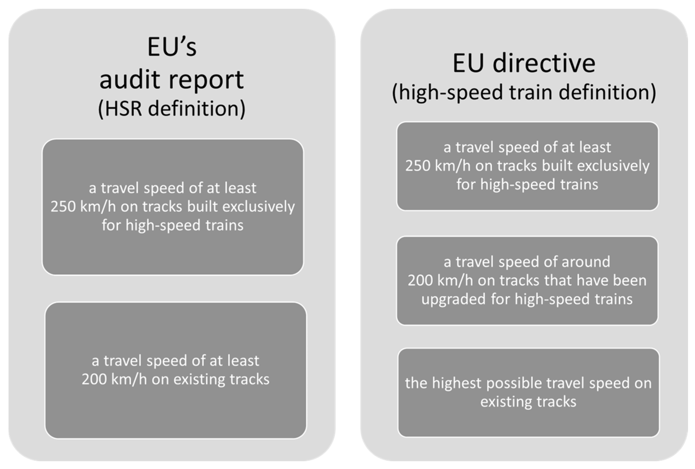
The European Union’s audit report [3] defines HSR as a service operating on specially designed tracks, where a travel speed of at least 250 km/h is achieved, and on existing tracks, where a travel speed of at least 200 km/h is achieved (Figure 1). The European Union directive [10] defines a high-speed train as a train that enables safe and continuous travel at a travel speed of at least 250 km/h on tracks built exclusively for high-speed trains, at a travel speed of around 200 km/h on tracks that have been upgraded for high-speed trains, or at the highest-possible travel speed on existing tracks. Typical travel speeds for high-speed trains are listed in [11]. In Italy, the Frecciarossa high-speed train can reach speeds of up to 300 km/h; the Frecciargento high-speed train, up to 250 km/h; and the Frecciabianca high-speed train, up to 200 km/h [11]. As our case is based on the example of Sweden, we need to mention that Sweden’s SJ high-speed train can reach speeds of up to 200 km/h [11].

Let us focus on the phrase minimum travel speed. If we check the list of HSR operators in Europe, we can find that the high-speed train of the SuperCity HSR operator, which connects the Czech Republic and Slovakia, only reaches a travel speed of up to 160 km/h and not at least 200 km/h [11]. Therefore, the definition of the high-speed train from the European Union directive is more appropriate. HSR lines can also be defined in a manner similar to that of the high-speed train. The European Union directive categorizes HSR lines into three categories: lines built exclusively for high-speed trains, allowing for travel speeds of at least 250 km/h; lines upgraded for high-speed trains, allowing for travel speeds of up to 200 km/h; and lines upgraded for high-speed trains, where the travel speed depends on the geographical characteristics of the area. For the purposes of this study, we will consider the latter definition.

1.2. Related Work

Published research mostly focuses on competition between individual modes of transportation within or between major cities or international hubs. Our review is focused on articles considering air and train route choices.

Individual preferences for travel alternatives are usually analyzed and estimated with demand models. Discrete choice models, aligned with consumer theory, are ideal for this purpose [12]. These models assume that travel decisions are influenced by the characteristics of the available alternatives. Many researchers are focusing on passenger travel mode choices using regression models [6,7], multinomial logit models [13,14,15], nested logit models [16], or models based on system dynamics [17]. A lot of attention has also been given to macroscopic traffic flow modeling (e.g., [18]).

Although our focus is on middle-distance transportation, it is important to note that regression and logit models are also commonly employed in mode decision making within urban passenger transportation. Berrill and others [19] argue that travel distance is commonly the most important feature for mode choices. Analyses for European cities show that there are lower likelihoods of walking and using public transit in low-density neighborhoods [19]. Because Europe has many areas lacking in train connections (especially in Eastern Europe), we expect that travel from short to middle distances will be, in some parts of Europe, carried out predominantly by road transportation.

The high-speed train’s potential to compete with airplanes on the Madrid–Barcelona route is evaluated in [5]. Using experimental design techniques, it models passenger preferences and estimates a logit model to analyze choices between the airplane and the high-speed train. The findings suggest a significant impact on the airline market, with many passengers switching to the train. The research targets current airplane travelers on the Madrid–Barcelona route, evaluating the train’s impact on airline demand. The key variables include travel cost, travel time, access time, and service frequency.

Albalate et al. [6] find direct competition between HSR and airlines, but there is also evidence that HSR can support long-haul air services, especially in hub airports with HSR stations. Their study uses route–year pairs as the unit of observation, collecting data for 180 routes over nine years for flight frequencies and eight years for the number of seats. Transportation lines between locations within Spain, France, Italy, and Germany were considered. The analysis examines the impacts of various factors, such as the population, GDP, distance, hub status, presence of HSR, market concentration, and low-cost carriers, on the total number of seats and the total annual frequency of flights provided by airlines.

It is a different situation in other European countries. For example, Germany’s HSR network is less centralized in one city with a hub airport because Germany has many larger cities connected with airports and not with HSR. Also, there are many geographical characteristics (e.g., the Alps in Switzerland, lakes in Finland and Sweden, and non-existent infrastructure in Eastern Europe) that prevent trains from reaching higher travel speeds. Another fact is that HSR services are carried out by individual country operators and are mostly not connected between different countries. Although individual lines (e.g., Madrid–Barcelona and Paris–Lyon) are highly beneficial financially and timewise, the lack of connectivity for travel between countries presents a significant challenge.

Although much of the research is focused on small geographical areas, usually considering existing HSR lines and/or air routes, there is also some focus on travel mode choices in urban mobility systems (e.g., [15]). Logit or discrete choice models naturally describe these situations well, but when we consider a larger geographical area, alternative approaches may prove to be more suitable.

In this paper, we will present a model that will help us to make transportation choices across a chosen geographical area. We will build a simple choice model and a network dataset, where we will not seek mode decisions between a pair of points (e.g., on existing lines) but a set of points. Such a model may provide policymakers with various analyses, which can contribute to more consistent decisions when creating policies and building infrastructure.

2. Materials and Methods

2.1. Data

When building a choice model, we aimed to create one that is more general than the existing ones. It should be applicable to larger geographical areas and capable of providing decisions for a set of arbitrary chosen points rather than being restricted to the existing HSR lines or airways. In the first attempt at finding a solution, the model is tested from the time-based perspective, where the fastest route in each part of the whole tour represents the optimal state of the model. The results from this modeling approach provide valuable insights and can greatly assist policymakers in making informed decisions about where and how to implement initiatives for transitioning to rail travel.

Using publicly available data [20], we built a network dataset—a multimodal network of Sweden, in ArcGIS Pro software, version 3.3.1. The multimodal network included road, rail, and air transportation modes. Sweden was chosen because of its existing system of HSR and domestic air travel. As a basis for constructing the multimodal network, we used the line layer of the Swedish road network [20]. As lines, we added 17 HSR connections and 41 air connections. For the list of HSR connections, we used the list of HSR operators listed in [11], the Omio portal for the travel times of train connections [21], and the Flight Connections portal for information on airline connections and their travel times [22]. These connections were created manually, one at a time, using the Create tool. To distinguish between different modes of transportation, we linked each connection in the multimodal network with information about the mode of transportation that can operate on it. If a connection in the multimodal network was a part of the road network, we labeled it as Road; if it was a part of the HSR network, we labeled it as Rail; or if it represented a connection between selected airports, we labeled it as Air. To ensure connectivity between different modes of transportation, we added additional lines representing connections between given modes of transportation, e.g., a connecting road between the existing road network and the airport, which also served as the starting/ending point for air connection to/from that airport. Additionally, we added 13 HSR stations and 29 airports, based on data from [11,22].

Then, we focused on generating a grid of evenly distributed points to explore the possibility of using either airplanes or high-speed trains for travel. Sweden’s border served as the boundary for the distribution of points. Using the Create Fishnet tool, we generated a grid of evenly distributed points covering the area within, based on the polygon layer—a grid of cells measuring approximately 40 km wide and 110 km long.

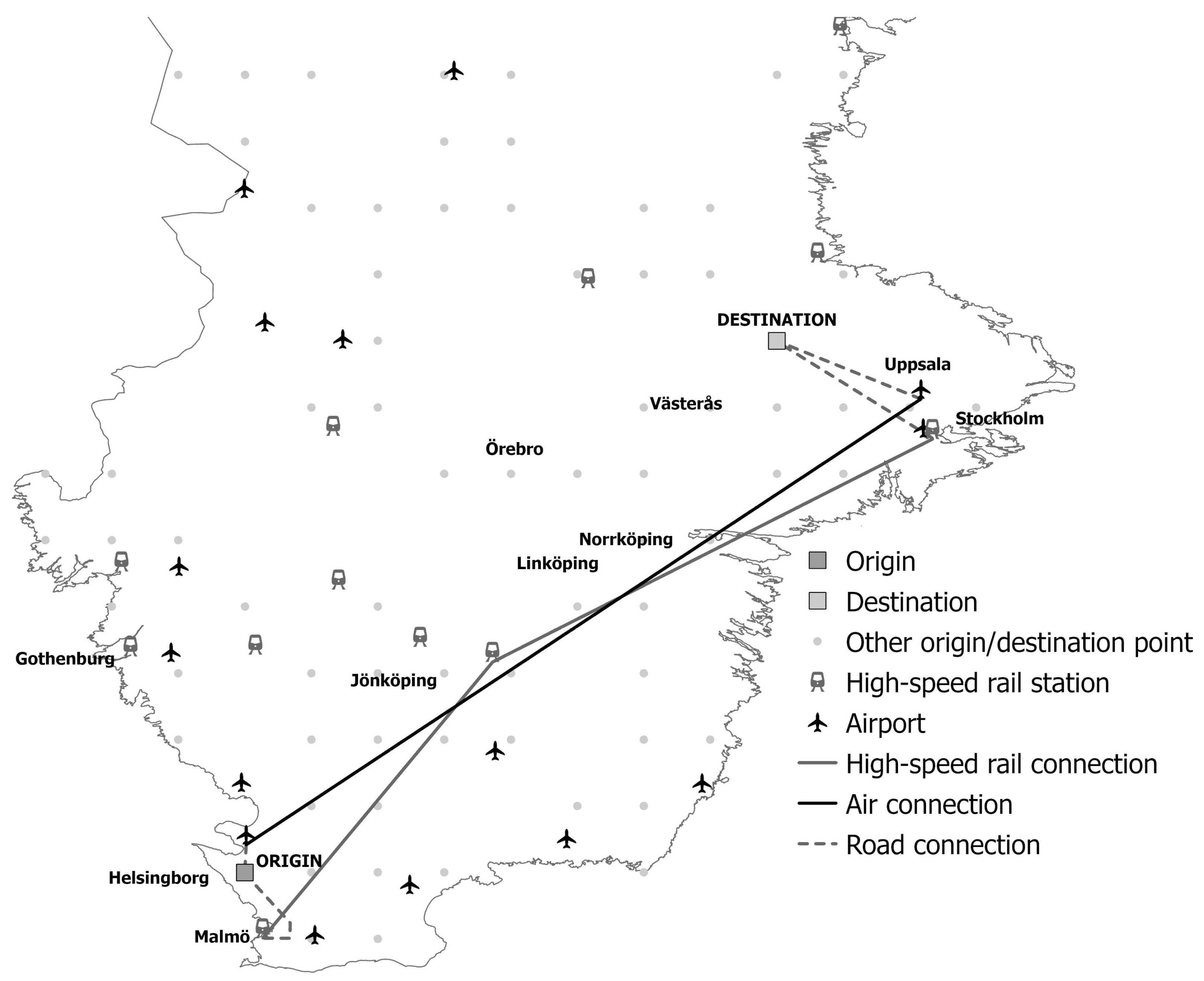
At first, however, we had to adjust the initial selection of points. Arbitrary points, as the starting points of the journey, were selected as in Mepparambath et al. [23], where they used clustering to obtain a smaller set of locations/polygons representing origins and destinations of journeys. They assumed that passengers begin and end their journeys in polygons representing buildings. Therefore, among the set of polygons representing origins and destinations, they retained areas representing areas of buildings while excluding areas representing green spaces, water bodies, and transportation infrastructure. After excluding these areas from the dataset, unevenly distributed polygons remained. To establish a uniform distribution of polygons, the DBSCAN clustering algorithm, a density-based clustering tool in ArcGIS Pro, was used. By considering this aspect of accessibility, we obtained a final set of 126 points (locations). For each of these locations, we determined the preferred mode of travel to all the other locations within a given distance. In Figure 2 we present a sample of the constructed multimodal network, showing rail and air travel between two locations.

Travel times were used as the focal parameter in the analysis. For the part of the multimodal network that includes the road network, the time required to travel across each connection was obtained through the predetermined speed of travel on each road segment [20]. Flight times of airplanes were used for air connections [22] and travel times of high-speed trains for HSR connections [21]. When entering times for high-speed trains and airplanes, we also considered check-in times, specifically, 120 min for air connections and 30 min for high-speed trains [24]. Examples of travel times between origins and destinations are listed in

Table 1. Examples of travel times between origins and destinations.

Type	Origin	Destination	Travel Time
HSR connection	Stockholm	Goteborg	3 h
Air connection	Stockholm (Arlanda)	Goteborg	1 h 5 min
Air connection	Stockholm (Bromma)	Goteborg	1 h 5 min
HSR connection	Stockholm	Malmo	4 h 26 min
Air connection	Stockholm (Arlanda)	Malmo	1 h 15 min
Air connection	Stockholm (Bromma)	Malmo	1 h 20 min

.

2.2. Research Approach

The preferred mode of travel was chosen from high-speed train, airplane, or a combination of those two modes. If there was no option to include any of the given transportation modes in the route, we listed it as “other”. To conduct the analysis, we chose distances of up to 100 km, 200 km, 300 km, 400 km, 500 km, 600 km, 700 km, 800 km, 900 km, and 1000 km from the starting location.

First, we selected a starting location (origin) from one of the 126 generated points. Using the predetermined radius, we then determined how many other locations could be reached from the starting location, thereby creating a selection of points representing potential destinations. Using the created multimodal network as a data source, we performed analyses to find the fastest routes between the origin and each destination separately. The selection of points was performed within the predetermined radius in which real distances and travel times are used.

For route analysis the Network Analyst extension of the ArcGIS Pro program was used. We considered the condition that both the origin and the destination station/airport of the HSR/air connection must be within the given radius. After each analysis, we determined chosen modes of transportation for each route by reviewing the Show Directions document. If an airplane was used on a route, we marked that route as including air travel (Air). If a high-speed train was used on a route, we marked that route as including high-speed train travel (Rail). If both an airplane and a high-speed train were used on the same route, we marked that route as including a combination of both (Combination). If the route did not include either a high-speed train or an airplane, we categorized it as “other” (Other). Road transportation was used just as the support mode to fill in the gaps caused by non-existing public transportation on a certain part of the route. We also assumed that we can seamlessly switch from one transportation mode to another. To focus on the competition and complementarities between air and HSR services, the sample excludes air routes with an island as a starting point or an endpoint.

We wanted to determine a preferable mode of transportation for each point. For each equidistant point within a given radius, we first summed up the number of each mode of travel that occurred. Then, we looked for the mode of transportation with the highest total value to determine the dominant mode of transportation within a given radius. To determine the breakeven point, we used the data of the shape areas of Voronoi diagrams, a polygon layer based on a point layer, representing 126 locations. We summed the values of the shape areas of Voronoi diagrams for each mode of transportation within a specified radius. The results are discussed and presented as graphs and maps.

2.3. Advantages and Disadvantages of Using ArcGIS Pro

The flexible use of ArcGIS Pro is one of its advantages. It allows us to independently construct and customize the network dataset while effectively displaying results. Additionally, it is a highly versatile cartographic tool, making the visualization of numerical data straightforward and efficient.

However, the use of ArcGIS Pro did come with certain drawbacks. A notable challenge was the time-intensive nature of preparing the network dataset and conducting analyses. Despite consulting with companies specializing in ArcGIS Pro, we were unable to accelerate the analysis process because of the complexity of the problem being addressed. Another significant limitation was the availability of the necessary data layers. During the research, we discovered that layers needed for our analysis were simply not yet developed or available.

To compare travel times between different modes of transportation, using route planners, like Google Maps, would be more effective. In our case, the network dataset was configured to present us with the fastest travel mode for each segment of the route as the (partial) result of the analysis. If we wanted ArcGIS Pro to provide a comparison of travel times for the same route across different modes, it would be more efficient to use a route planner. Conducting such analyses in ArcGIS Pro would significantly increase the processing time, as each route would require at least four analyses (road, HSR, airplane, and the fastest route).

2.4. Model

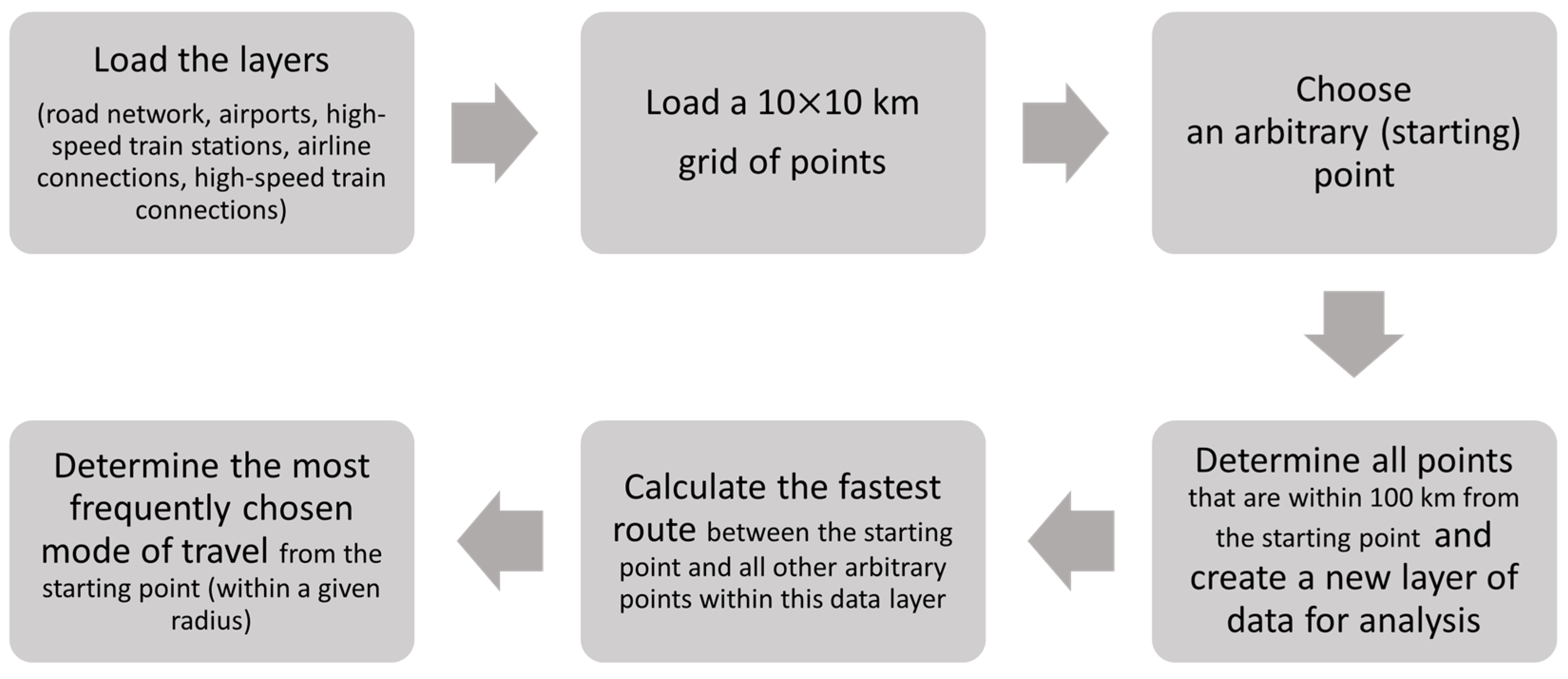
In the first attempt at finding a solution, we built a simple choice model that is performed in 6 steps. In the first step, we load relevant layers into the program (road network, airports, high-speed train stations, airline connections, and high-speed train connections). In the second step, we load a 10 × 10 km grid of points; then, we choose an arbitrary (starting) point on the grid (step 3). In step 4, we determine all the points on the grid that are within 100 km from the starting point and create a new layer of data for the analysis. In step 5, we calculate the fastest route between the starting point and all the other arbitrary points within this data layer. This process is repeated until we determine all the routes between the starting point and all the other points within the selection. Obviously, this indicates the model’s complexity and the use of difficult solution procedures, as it can be hard even to find all the feasible solutions. We would like to emphasize that the model is in the starting phase and should therefore be reasonably reconstructed. But first of all, let us introduce the notations that are represented in this simple modelling approach (

Table 2. Notations.

$P$	set of equidistant geolocations
$P_0$	origin (starting) point $\in P$
$P_d$	destination point $\in P$
$A_0$	airport nearest to $P_0$
$R_0$	train station nearest to $P_0$
$A_d$	airport nearest to $P_d$
$R_d$	train station nearest to $P_d$
$t_{ac}$	2 h airport check—in time
$t_{rc}$	0.5 h railway check—in time
$t_{au}$	0.5 h airport baggage claim and exit
$t(i,j)$	travel time between origin point $i$ and destination point $j$
$t_r$	travel time by road transportation between $P_0$ and $P_d$
$T_{rr}$	total travel time by railway transportation between $P_0$ and $P_d$
$T_a$	total travel time by air transportation between $P_0$ and $P_d$

).

In this analysis, we need to calculate the total travel time using railway transportation (Equation (1)) and air transportation (Equation (2)).

$$T_{rr}\left(P_o, P_d\right)=t\left(P_o, R_o\right)+t_{rc}+t\left(R_o, R_d\right)+t\left(R_d, P_d\right) \mathrm{a}\mathrm{n}\mathrm{d}$$

(1)

$$T_a\left(P_o, P_d\right)=t\left(P_o, A_o\right)+t_{ac}+t\left(A_o, A_d\right)+t_{au}+t\left(A_d, P_d\right).$$

(2)

In step 6, we determine the most frequently chosen mode of travel within a given radius of the starting point (based on the previously determined mode of travel between the selected points). We calculate the number of times each mode of transportation occurred within a given radius. The mode with the highest value is a preferable mode of transportation for this current starting point within a given radius. Then, we move on to the next point and repeat steps 3, 4, 5, and 6. We complete the analysis for all the points within a given radius and then continue this process for all the predetermined radii. The pseudocode of the modeling procedure is provided in

Table 3. Pseudocode.

for r = 100 km to 1000 km

r1 = r

r2 = r + 100 km

for each $P_o$ in $P$ do

for each $P_d$ in $P$ where $r1<distance\left(P_o, P_d\right)<r2$

if $T_a\left(P_o. P_d\right)<T_{rr}$ then

$P_o\left[r\right].preference=airport$

else if $T_a\left(P_o. P_d\right)>T_{rr}$ then

$P\left[r\right].preference=railroad$

else if $t_r\left(P_o, P_d\right)<T_{rr}\left(P_o, P_d\right) \mathbf{a}\mathbf{n}\mathbf{d} t_r\left(P_o,P_d\right)<T_a\left(P_o, P_d\right) \mathbf{t}\mathbf{h}\mathbf{e}\mathbf{n}$

$P\left[r\right].preference=other$

end

end

r = r + 100 km

end

, and a schematic view is given in Figure 3. With travel duration being the goal, the main parameter affecting the presented model is time, which encompasses both travel times as well as check-in times. The optimal state of the model, thus, represents the fastest route in each segment of the journey.

As mentioned in Section 2.2, air travel was chosen in the segment of the journey if its travel time plus the airport check-in time was shorter than the corresponding times for HSR or other means of transportation (see also Pseudocode in Table 3). Because we focused on competition between HSR and air travel, we used other means of transportation (e.g., road transportation) where public transportation is not available on a given route. Although this case considers competition between an airplane and a high-speed train, the proposed model currently considers just the time parameters. Regardless of the mode of transportation considered, the winner will be the one that is the fastest. In some regions, the absence of railway infrastructure or air connections might mean that road transportation will represent the more advantageous and favored mode for medium travel distances because it may represent the fastest transportation option.

In

Table 4. Example of travel times between chosen origin and destination points.

Route	Notation	Distance	Time
Origin–Destination	$P_o, A_o$	34.5 km	40 min
	$A_o, A_d$	476 km	2 h 25 min
	$A_d, P_d$	136.5 km	2 h 35 min
		647 km	5 h 40 min
Origin–Destination	$P_o, R_o$	256 km	4 h 27 min
	$R_o, R_d$	540 km	3 h 21 min
	$R_d, P_d$	166.85 km	3 h 11 min
		962.85	10 h 59 min

, we present the calculated traveling times for the example from Figure 2 (arbitrarily chosen origin point, with coordinates at (12,847,778, 56,098,956), and destination point, with coordinates at (16,873,509, 60,068,049)). We need to note that we are providing this calculation solely for clearer presentation purposes. As mentioned above, such analyses are included in the procedure but are not reflected in the outcomes, as performing them would significantly increase the software’s processing time. It is worth noting that in this case, the airplane is the fastest option, representing the quickest route for the entire journey between the chosen origin and destination points.

3. Results

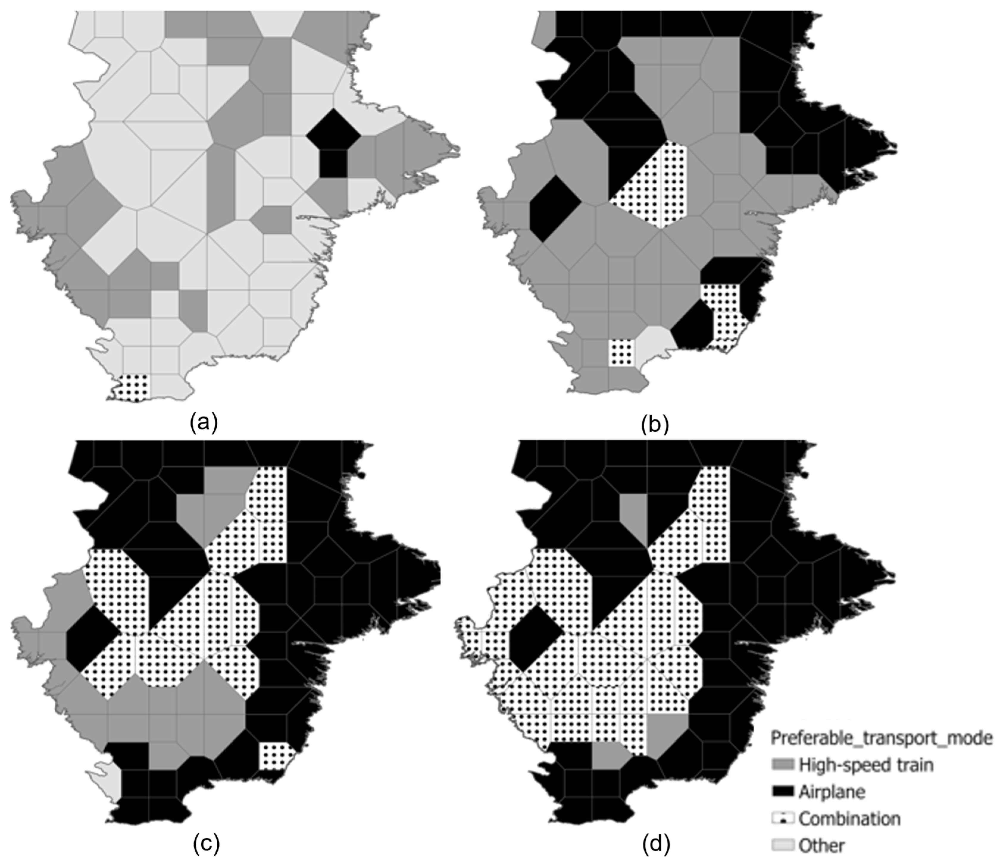
We performed more than 9000 route analyses between all the generated points. Figure 4 represents the chosen transportation mode for generated points within radii of 200, 400, 600, and 800 km. For points within a radius of up to 100 km, the results show that neither the high-speed train nor the airplane nor the combination is chosen (see also Figure 5), and for points within a radius of beyond 800 km, the airplane emerges as the most frequently chosen mode of transportation.

As seen in Figure 4a, within a radius of up to 200 km, the most frequently chosen transportation modes are high-speed train and “other”. Figure 4b represents the radius of up to 400 km. Herein, in some cases, the chosen modes of transportation are the airplane and combination, but the dominant mode of transportation is still the high-speed train. The situation differs in Figure 4c, which represents the radius of up to 600 km. Herein, the airplane becomes dominant. Further, air transportation and the air/rail combination are mostly chosen, while the high-speed train mode appears just in a few cases (Figure 4d). We may also highlight that for a radius of up to 1000 km, the airplane mode appears in almost all the cases.

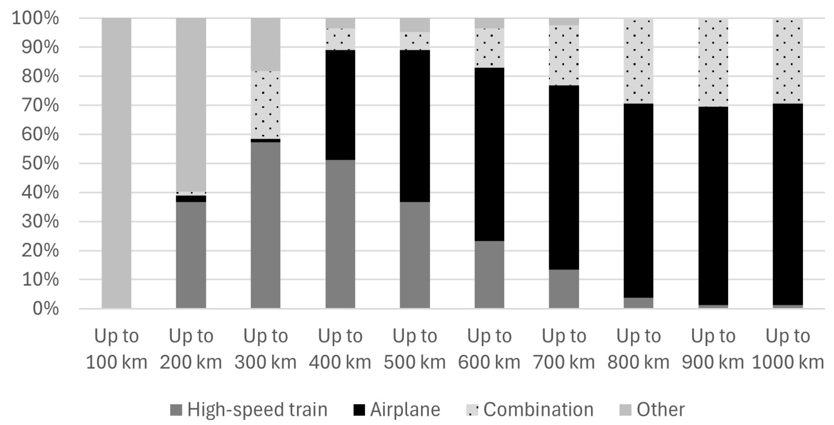
A similar pattern can also be seen in Figure 5, which represents the share of each transportation mode within each tested radius. It is clearly visible that within 100 km, just the “other” transportation mode is chosen and that this type of transportation is rarely represented within a radius of up to 700 km. The high-speed train is selected within the radii from up to 200 km to up to 800 km. The combination of the airplane and high-speed train appears to a lesser degree within a radius of up to 200 km and is mostly represented within radii longer than 600 km. Similarly, the airplane is first noticed on routes that are within radii of 200 km and 300 km. The air transportation mode becomes dominant on routes beyond 400 km.

If we compare the results shown in Figure 2 and Figure 4, we can claim that HSR stations are much more present in inner areas that connect densely populated areas. Therefore, we may expect that air travel alone will be chosen for border areas and in combination with high-speed trains in inner areas. From Figure 5, we can see that as the distance increases, the shares of “other” and high-speed trains decrease, the share of airplanes increases, and the share of the combination emerges between 200 km and 300 km, as it depends on which mode of transportation is the fastest in a given segment of the journey. In terms of the travel distance and, consequently, time, the air transportation mode represents a better option (compared to the high-speed train and “other” modes of transportation).

From more than 9000 route analyses performed for the case of Sweden, we can determine the breakeven point between HSR and air travel. For the tested radii from 100 km to 1000 km, we obtained results of how many times different transportation modes appear in solutions.

4. Discussion

Figure 6 represents the breakeven point between air travel and HSR travel, based on the aggregate number of chosen transportation modes within each radius. We need to highlight that breakeven point is represented just for airplanes and high-speed trains because our idea is to show when it is reasonable to shift passenger transportation at middle distances from airplanes to railways. From the represented surface area (in percentages) in Figure 6, we may observe that up to 400 km, it is worthwhile to travel by high-speed train, and for the distances longer than 400 km, it is much more convenient to use the air transportation mode in the case of Sweden.

The usefulness of the presented model lies in its ability to immediately identify areas where the dominant mode of transportation is sustainable and where it is not. Therefore, it gives us the possibility of a much broader application range. It allows us to identify those areas where a particular mode of transportation is already well developed and integrated into commuting while also identifying those modes of transportation that need to be further integrated into those areas’ transportation system. Despite Sweden’s well-developed HSR network connecting major cities, it is important to recognize that air travel often prevails in these regions because of the extensive aviation infrastructure, which offers superior time efficiency. This underscores the need to incorporate additional decision-making factors and to expand the model to a multiobjective decision analysis framework capturing a broader range of considerations beyond time and emissions alone.

As of now, the model enables us to determine, for any point in a given area, whether it is more advantageous to travel by train or by airplane based on the time spent traveling from that point, whether it is in an urban area or in a sparsely populated rural area. Furthermore, it provides this information in relation to the distance to the intended destination. As demonstrated by the example of Sweden, we can observe that the breakeven distance is not constant and varies depending on several different factors, which should be identified and investigated further in the future. This information can be of great assistance to policymakers in making informed decisions on where and how to implement initiatives for transitioning to rail travel. In addition to mitigating the negative environmental impacts of certain transportation modes, it can also serve as a valuable tool for sustainable planning, facilitating the strategic development of infrastructure, industrial zones, residential areas, and other key urban and regional features.

Although we are currently considering only time parameters, this does not diminish the model’s valuable outcomes. Even as the model is upgraded to include various factors, the resulting figures will continue to support strategic decisions. For the same case of Sweden, it will be intriguing to examine how sustainability factors might alter the breakeven distance.

5. Conclusions

In this paper, we presented a time-based breakeven distance analysis between HSR and air travel. The analysis was conducted for Sweden because of the presence of high-speed trains and domestic air transportation. It was shown that in Sweden, it is worthwhile to travel by high-speed trains for distances of up to 400 km and for greater distances, by air transportation.

The used mathematical model presents a basis for future research of European travel preferences. The resulting figures reveal that in the eastern regions of Sweden, air travel outperforms HSR. This modeling approach provides visual insights that can be further analyzed from demographic, infrastructural, and other relevant perspectives. This enables us to assess the development level of specific travel infrastructure and, in turn, understand why air travel dominates over HSR in the eastern part of Sweden.

Currently, this modeling approach presents a well-defined proof of concept. With the presented model, it is possible, for any chosen area, to define the breakeven distance, depending on various factors (e.g., geographical features and existing infrastructure). The same model can be used for any mode of transportation, not just for trains or airplanes. Building a model that illustrates the distribution of decisions across a broader geographical area—considering various factors, such as infrastructure development, GDP, and the purchasing power of the population—would be a valuable avenue for future research.

In future research, we will expand this study to a broader area of multiple countries with the aim to find differences in the breakeven points. Further improvements to the presented model will include other criteria that influence passenger mode choice, ranging from the cost perspective to personal preferences. The idea is to introduce a preference factor that will consider direct factors (e.g., distance, time, and travel costs) and indirect factors (e.g., comfort of travel, connectivity, and sustainability). Once the model is refined, we anticipate that travel time will no longer have the upper hand over environmental considerations (negative impacts). Instead, it will provide solutions that align with a balanced set of decision preferences, integrating both sustainability and efficiency.

To increase the competitiveness between different transportation modes, it is of the utmost importance to identify areas where it is reasonable to invest in infrastructure. The findings of such research will be of great importance for policymakers because the results of the analysis conducted clearly illustrate the actual situation. The rail transportation mode is the preferable one in areas with well-developed railway infrastructure and train connections. For example, in some parts of Eastern Europe, where passenger traffic is poorly developed, it is expected that the use of personal vehicles will be the most common choice for passenger travel. Such a presentation of the current situation reveals opportunities and, so, facilitates decisions when making development strategies for future investments.