Abstract
Global warming, driven by greenhouse gas (GHG) emissions, is accelerating globally and highlights the need for effective mitigation strategies. This study assesses the economic feasibility of rainbow trout aquaculture by incorporating GHG emissions into its analysis, thereby contributing to mitigation efforts in the fisheries sector. Focusing on two farming systems—recirculating aquaculture systems (RAS) and flow-through systems (FTS)—we estimated GHG emissions and conducted an economic evaluation using data collected through field surveys. The average GHG emission was 7.14 kg CO2 eq per kilogram of trout produced, with RAS showing lower emissions than FTS. Electricity and feed were identified as the primary emission sources. The economic analysis revealed an average net present value (NPV) of USD 987,609 and an internal rate of return (IRR) of 18%, with RAS outperforming FTS in profitability. A sensitivity analysis under carbon pricing showed that economic feasibility was maintained, but the NPV declined by about 24% under the carbon tax scenario. Overall, these findings underscore the importance of balancing profitability and emission reduction for sustainable aquaculture management.
1. Introduction
Since the Intergovernmental Panel on Climate Change (IPCC) released its Special Report on Global Warming of 1.5 °C [1], countries around the world have actively pursued efforts to limit the rise in global average temperature to below 2 °C. In line with these efforts, South Korea announced its “2050 Carbon Neutrality Strategy” in 2020, reaffirming its commitment to reducing greenhouse gas (GHG) emissions as part of the international community [2].
The Ministry of Oceans and Fisheries (MOF) of South Korea introduced the “2050 Carbon Neutrality Roadmap for the Marine and Fisheries Sector”, aiming not only to reach net-zero emissions by 2050 but to achieve a reduction of 3.24 million tons below zero. This roadmap organizes GHG reduction efforts into five key categories: shipping, fisheries and fishing villages, marine energy, blue carbon, and ports.
For the “fisheries and fishing villages” sector, the target GHG emissions by 2050 have been set at 115,000 tons. In contrast, emissions in 2018 were approximately 3.04 million tons, including 2.54 million tons of direct emissions and 504,000 tons of indirect emissions. While direct emissions—mainly from fuel use in fishing vessels—have been gradually declining, indirect emissions from electricity consumption in aquaculture facilities have been increasing [3,4].
In this context, identifying GHG emission sources from aquaculture and accurately estimating their volume is becoming increasingly important, particularly given the rising share of aquaculture in total fisheries production. Although several studies have addressed GHG emissions in Korean fisheries [5,6], only a few have examined aquaculture, focusing mainly on seaweed, eel, and flounder aquaculture [7,8,9]. However, these works are relatively dated, and recent research on aquaculture GHG emissions in Korea remains scarce.
Beyond estimation, it is also essential to evaluate the economic impact of GHG emissions and develop corresponding strategies. Many international organizations recommend carbon pricing policies as effective tools for GHG mitigation [10]. Although no such pricing mechanisms currently apply to aquaculture in South Korea, under the “polluter pays” principle, the industry may be subject to future regulations [11]. This study, therefore, estimates GHG emissions from aquaculture and examines the economic feasibility of incorporating environmental costs based on carbon pricing mechanisms.
Specifically, this study focuses on rainbow trout aquaculture—an important inland industry—by comparing recirculating aquaculture systems (RAS) and flow-through systems (FTS). RAS is recognized as an eco-friendly method that filters and reuses water and is expected to play an increasingly important role in adapting to climate change impacts such as rising temperatures [12]. To assess whether RAS is environmentally sustainable in terms of GHG emissions, a comparative analysis with FTS was undertaken.
While several international studies have examined GHG emissions from trout aquaculture—such as those by d’Orbcastel et al. [13] and Samuel-Fitwi et al. [14]—their reported values differ substantially across farming systems and contexts. However, no comparable research has been conducted in South Korea. Regarding economic aspects, Baek and Park [15] examined the feasibility of trout aquaculture and found generally favorable profitability.
Based on this context, the present study quantifies GHG emissions from eight trout farms, evaluates their economic feasibility across aquaculture methods, and examines the implications of carbon pricing by incorporating environmental costs, thereby providing insights to guide sustainable aquaculture management.
2. Trout Aquaculture
Rainbow trout (Oncorhynchus mykiss) is the predominant species in trout aquaculture in South Korea. As a cold-water species belonging to the order Salmoniformes and family Salmonidae, rainbow trout requires consistently low water temperatures throughout the year. Consequently, trout farming is primarily concentrated in regions such as Gangwon-do, Chungcheongbuk-do, and Gyeongsangbuk-do, as shown in Figure 1.
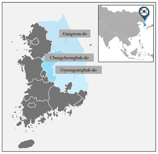
Figure 1.
Map of trout farming region in South Korea.
Over the past decade, annual trout production has averaged around 3000 tons, peaking at 3390 tons in 2013 and subsequently fluctuating to reach 2757 tons in 2023 (Figure 2) [16]. In terms of economic value, trout aquaculture ranks second among inland water species in South Korea, following eel, with an average annual production value of approximately USD 21.7 million and a recorded value of USD 29.3 million in 2023 [16].
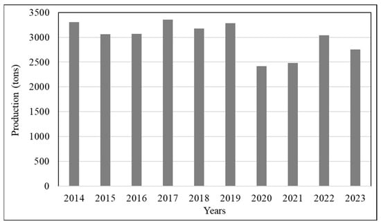
Figure 2.
Production of trout aquaculture in South Korea (tons).
Trout aquaculture in South Korea utilizes both flow-through systems (FTS) and recirculating aquaculture systems (RAS). According to a 2018 survey, of the 154 registered trout farms, 147 employed FTS and only seven adopted RAS [17]. While FTS remains the dominant method, it is typically characterized by conventional system designs that rely heavily on natural water sources and are often associated with aging infrastructure. In contrast, RAS farms are considered modern, eco-friendly systems capable of maintaining controlled aquaculture environments. These systems support high-density production and enable more effective management of effluent discharge, making them increasingly favorable in sustainable aquaculture development.
3. Materials and Methods
3.1. Trout Farms Field Survey
In this study, eight trout farms—five employing flow-through systems (FTS) and three using recirculating aquaculture systems (RAS)—were selected based on strict criteria, including aquaculture method, geographic location, farming period, and stocking and harvesting sizes. Field surveys were conducted from May to July 2022 to collect data on the use of greenhouse gas (GHG) emission sources, as well as production costs and revenues.
Table 1 presents the characteristics of the surveyed farms. The average water surface area of FTS farms was 2722 m2, with an average stocking of 68,333 fry. Their survival rates ranged from 80% to 90%, and total production varied between 20,000 kg and 80,000 kg. In comparison, RAS farms had an average surface area of 2431 m2 and an average fry stocking of 76,000, with survival rates ranging from 77% to 90% and production between 45,000 kg and 100,000 kg.

Table 1.
Trout farms field surveys.
All surveyed farms typically stocked fry weighing approximately 5 g. The fry were either directly purchased or raised from externally sourced eyed eggs before being stocked. While some farms shipped trout in a range of sizes from 1 kg to 3 kg, most shipped fish weighing between 1.0 kg and 1.2 kg per individual.
The market price of trout ranged from USD 8.31 to USD 10.09 per kilogram. Compared to previous findings by Baek and Park [15], which reported prices ranging from USD 5.00 to USD 7.69, the current prices represent a significant increase. In 2021, the average market price of trout per kilogram was approximately USD 6.15; however, beginning in November 2021, prices started to rise steadily, eventually stabilizing around USD 10.09 between January and July 2022 [18]. This increase has been attributed to a rise in demand following the relaxation of COVID-19 social distancing measures, combined with a limited supply caused by reduced production volume [19,20].
3.2. GHG Emissions Estimation
The list of emission sources related to aquaculture is referred to as the GHG inventory, which serves as the basis for estimating total emissions in this study. To estimate GHG emissions from trout aquaculture, this study constructed a GHG inventory based on prior research [9,21,22,23,24]. As shown in Figure 3, emissions were divided into those generated during the farming process—such as electricity, fuel, feed, liquid oxygen, and infrastructure—and those generated during transportation, including fry transport and shipment of market-size fish.
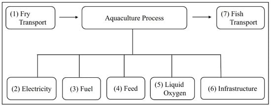
Figure 3.
GHG inventory of trout aquaculture.
The GHG emission calculation grade, known as Tier, indicates the level of methodological complexity and data specificity in the estimation process. This study followed the Tier 1 approach from the Intergovernmental Panel on Climate Change (IPCC) guidelines, which relies on default emission factors [25], as region-specific Tier 2/3 parameters for Korean aquaculture are not currently available. The basic formula involves multiplying activity data (AD) by the emission factor (EF) and the global warming potential (GWP) of each gas [26].
Emission sources were categorized into energy and non-energy sectors. The energy-related sources included (1) fry transport, (2) electricity, (3) fuel, and (7) fish transport (Figure 3). These sources produced direct emissions of CO2, CH4, and N2O due to fossil fuel combustion, and indirect CO2-equivalent emissions from electricity consumption [25]. The specific emission equations for each gas type were based on guidelines from the Energy and Greenhouse Gas Comprehensive Information Platform [27] and the 2021 National Greenhouse Gas Inventory Report [25], as shown in Equations (1)–(3):
In Equation (1), denotes the fuel supply (replaced by fuel usage in this study), represents the net calorific value, and is the carbon emission factor. The constant 10−6 converts emissions to kilograms, while 44/12 adjusts carbon to CO2 emissions. In Equations (2) and (3), is the conversion factor, (CH4) and (N2O) are the respective emission factors, and 41.868 converts the TOE calorific unit into joules [6,11,25].
GHGs CH4 and N2O were converted into CO2-equivalent units using global warming potentials (GWPs) of 21 and 310, respectively. For electricity, which is an indirect source of emissions based on consumption, an emission factor of 0.4594 tCO2 eq/MWh was applied. This value had already been adjusted for GWP and was used by directly multiplying it with the electricity consumption.
Non-energy emission sources included feed, liquid oxygen, and infrastructure. Due to the absence of domestic emission factors for these sources, values per kilogram of use were adopted from previous international studies [14,28,29,30]. Emissions were calculated using the following formulas:
Here, is the activity data (amount used), is the emission factor, and refers to service life. Since previous studies reported data in CO2-equivalent units, no additional conversion was necessary. Total emissions per farm (kg CO2 eq) were obtained by summing all emission sources and dividing the result by the farm’s total production (kg), yielding emissions per kilogram of trout.
The materials required for GHG emission estimation included activity data, emission factors, conversion factors, and net calorific values. In this study, the system boundary of the GHG inventory encompassed the entire farming period, from the transportation of approximately 5 g fry from the hatchery to the shipment of 1 kg market-size trout to the distribution site. Emission sources that could not be quantitatively assessed due to data limitations—such as the eyed-egg production stage and wastewater treatment—were excluded from the inventory boundary.
Activity data for each emission source were collected through field surveys of eight trout farms and are summarized in Table 2. These data represent activity data in absolute terms for each emission source over one full farming period. On average, RAS farms showed higher electricity and feed consumption than FTS farms. All RAS farms relied entirely on electricity as their energy source, with no fuel usage.
Table 2.
Activity data of GHG emission sources.
For infrastructure, the amounts of concrete and plastic used in tank construction were converted. RAS farms required greater infrastructure material input than FTS farms due to the inclusion of additional filtration tanks.
Liquid oxygen was used to increase dissolved oxygen levels and enhance stocking density. However, some farms used mechanical devices, such as water wheels, instead. Fry and fish were generally transported within a one-hour radius, though transport frequency varied across farms.
The emission factors, conversion factors, and net calorific values in the energy sector were obtained from the National Greenhouse Gas Inventory Report [25], while the emission factors for non-energy sources were drawn from previous studies [14,28,29] (Table 3).
Table 3.
Emission factor, conversion factor, and net calorific value of GHG emission sources.
3.3. Economic Analysis
In this study, the economic viability of trout aquaculture was assessed based on the cash flows generated from production and management, as collected through field surveys. Key financial indicators—including net present value (NPV), internal rate of return (IRR), and benefit–cost ratio (BCR)—were employed to evaluate economic feasibility. NPV calculates the present value of net benefits by discounting future cash inflows and outflows, while IRR identifies the discount rate at which NPV equals zero. BCR expresses the ratio of the present value of benefits to the present value of costs. According to guidelines provided by the Ministry of Economy and Finance, a social discount rate of 4.5% was applied for a 10-year project period [31].
NPV, IRR, and BCR were calculated using the following formulas:
where represents the benefit at time , the cost at time , the discount rate, and the time period (Equations (7)–(9)). A positive NPV indicates economic feasibility, and among multiple options, the one with the highest NPV is considered most desirable. Similarly, an IRR higher than the discount rate suggests economic viability, and a BCR greater than 1 confirms that the benefits outweigh the costs.
Economic analysis was based on cost structures collected from eight farms, summarized in Table 4. Costs were categorized by percentage to enable comparison between farms with different production scales. The production period—from stocking fry to the shipment of adult trout—was approximately 12 months. All eight farms engaged in farming activities using eyed-eggs or fry procured externally, with costs ranging from USD 0.04 to 0.05 per eyed-egg and USD 0.23 to 0.31 per fry. Key cost items included feed and labor, which accounted for an average of 44.2% and 22.9% of total costs, respectively. Electricity, fuel, depreciation, and fry costs each ranged from 6% to 9%.
Table 4.
Operating expenses ratio for trout aquaculture (%).
Although FTS is generally considered more labor-intensive than RAS [32], labor costs were not significantly different between the two systems. This may be due to the fact that many FTS farms were operated solely by their owners, minimizing labor costs. RAS farms tended to have higher absolute electricity costs, although their proportional shares were lower or similar to those in FTS. This difference mainly reflects the energy-use structure: FTS farms combined electricity with diesel fuel, while RAS relied almost entirely on electricity. In addition, a few FTS farms showed markedly higher energy costs per unit of production, reflecting relatively low energy efficiency in those cases. Depreciation was generally higher in RAS farms, reflecting more advanced facility investments.
The environmental costs associated with trout aquaculture were calculated using the emissions trading system (ETS) and carbon tax within the context of a representative carbon pricing system. In South Korea, the ETS is currently in place. The average price of the Korean Allowance Unit (KAU) 21, recorded from 2 October 2021 to 30 June 2022, on the Korea Exchange Emissions Market Information Platform, stands at US$21/tCO2 eq [33].
The ETS permits businesses emitting greenhouse gases (GHG) to trade their surplus and deficit of allocated emission rights. Given that the ETS is not currently applied to the aquaculture industry in South Korea, determining the allocation of emission rights was not feasible. Consequently, this study applied the emission price to the total GHG emissions per farm, covering all identified sources. This comprehensive approach was adopted as a precautionary measure to evaluate the overall economic impact of potential carbon pricing on aquaculture operations.
The carbon tax is imposed on emitters who use carbon dioxide-emitting fuels such as coal and oil, based on their emissions. However, the carbon tax is not presently enforced in South Korea, and the International Monetary Fund recommends a rate of US$75/tCO2 eq [34,35].
4. Results
4.1. GHG Emissions Estimation
The estimated GHG emissions from trout aquaculture farms are shown in Table 5. Across the eight farms analyzed, total GHG emissions per farming period averaged 388 tons, ranging from 143 to 778 tons. The variation between Farm E, which recorded the lowest emissions, and Farm H, which recorded the highest, was primarily attributed to differences in production scale.
Table 5.
Estimated total GHG emissions by farm (kg CO2 eq).
Table 6 presents the GHG emissions per kilogram of trout produced (kg CO2 eq/kg), calculated by dividing each farm’s total emissions by its production volume. The average unit emission across all farms was 7.14 kg CO2 eq/kg, with values ranging from 4.26 to 12.33. Farm D exhibited the highest unit emissions, mainly due to elevated electricity use and reduced feed conversion efficiency relative to its production output. Specifically, the farm consumed 828,000 kWh of electricity for 45,000 kg of trout (18.4 kWh/kg) and used 70,000 kg of feed (FCR ≈ 1.57), both of which were less efficient than the cross-farm averages (≈9–10 kWh/kg and FCR ≈ 1.2). In contrast, Farm B recorded the lowest unit emissions, consuming 320,000 kWh for 80,000 kg of trout (4.0 kWh/kg) with 85,106 kg of feed (FCR ≈ 1.06), reflecting comparatively efficient utilization of energy and feed relative to its production level.
Table 6.
Estimated GHG emissions per 1 kg of trout by farm (kg CO2 eq).
Electricity and feed were identified as the primary contributors to GHG emissions, accounting for approximately 43–69% and 23–48% of total emissions, respectively. However, the relative shares varied considerably among farms. For example, Farms A and D exhibited a strong reliance on electricity, whereas feed-related emissions represented a larger proportion in Farm C. Farm E, although operating at a smaller scale and therefore generating relatively low absolute emissions, recorded unit emissions close to the overall average, indicating that scale alone does not determine efficiency. These results suggest that, while electricity and feed consistently dominate the emission profile, farm-specific management practices and production efficiency largely explain the variability in emission intensities across farms.
Most farms relied on electricity as their primary energy source, resulting in relatively low fuel-related emissions. Transportation-related emissions varied among farms but accounted for a small share overall, ranging from 1% to 6%. Emissions from other sources remained consistently minor.
GHG emissions by aquaculture method showed that although RAS farms exhibited higher total emissions than FTS farms, their per-unit emissions per kilogram of fish were lower (Table 7). This outcome highlights a trade-off: while RAS can be more efficient on a unit basis, scaling up production magnifies its absolute footprint.
Table 7.
Estimated GHG emissions by methods (kg CO2 eq).
4.2. Economic Analysis
The results of the economic feasibility analysis for both individual farms and aquaculture methods are summarized in Table 8. The average NPV was approximately USD 987,609, ranging from −USD 191,821 to USD 2,382,194. The average IRR was 18%, with values between −1% and 38%, while the average BCR was 1.31, ranging from 0.89 to 1.96. Farm B demonstrated the highest economic feasibility, which was attributed to its relatively low production costs. In contrast, Farm E, which had the lowest economic feasibility, was found to have relatively low production compared to its water area.
Table 8.
Economic analysis results by farms and methods.
At the method level, RAS farms outperformed FTS farms on average in terms of NPV, IRR, and BCR. This indicates that, despite variation among individual farms, RAS generally showed more stable economic outcomes under the surveyed conditions.
As a result of the economic feasibility analysis incorporating the ETS and carbon tax, economic performance declined compared to the baseline (Table 9). Under the ETS scenario, the average NPV, IRR, and BCR decreased by 7%, 6%, and 2%, respectively, whereas under the carbon tax, they fell by 24%, 22%, and 7%. These findings suggest that carbon pricing, particularly a tax-based scheme, could substantially weaken profitability.
Table 9.
Sensitivity analysis results by assuming the carbon pricing system.
5. Discussions
5.1. GHG Emissions Estimation
Electricity-related emissions arise mainly from water recirculation, pumping, and filtration, whereas feed-related emissions stem from the production, processing, and transportation of raw materials [36,37]. This aligns with previous studies identifying electricity, fuel, and feed as dominant contributors [21,22,23].
Despite this consistency, reported emission intensities vary. d’Orbcastel et al. [13] estimated 2.02 kg CO2 eq/kg for FTS and 1.60–2.04 kg CO2 eq/kg for RAS. In contrast, Samuel-Fitwi et al. [14] reported much higher values, with 3.56 kg CO2 eq/kg for FTS and 13.60 kg CO2 eq/kg for RAS. Dekamin et al. [38] likewise observed elevated emissions, estimating 1.16 kg CO2 eq/kg for FTS and 6.10 kg CO2 eq/kg for RAS. These discrepancies reflect differences in regional conditions, methodological assumptions, and inventory boundaries [23].
A key regional factor is the grid carbon intensity. In fossil-heavy grids such as Korea, electricity dependence drives emissions upward, whereas low-carbon grids in Europe yield lower intensities. For example, d’Orbcastel et al. [13] reported relatively low RAS values in France, consistent with its nuclear-dominated grid. By contrast, Samuel-Fitwi et al. [14] found substantially higher RAS emissions because energy use was about seven times greater than in FTS; even a low-carbon grid in Denmark could not offset high electricity demand. Instead, their sensitivity analysis further showed that switching to wind power reduced RAS emissions almost tenfold, underscoring the strong influence of grid carbon intensity.
These findings clarify the conflicting RAS–FTS rankings: when energy intensity is high and grids are carbon-intensive, RAS tends to exceed FTS; under very low-carbon grids or high farm efficiency, RAS can be competitive or even lower.
Methodological choices further contribute to variation. Our estimates are based on field-surveyed activity data from eight farms, to which we applied IPCC Tier-1 emission factors. By contrast, many earlier studies used modeled Life Cycle Assessment (LCA) inventories with different default parameters or exclusions [13,14,38]. For example, d’Orbcastel et al. [13] and Dekamin et al. [38] followed attributional LCA approaches, while Samuel-Fitwi et al. [14] applied a consequential LCA with system expansion that incorporated marginal energy assumptions. These contrasting frameworks illustrate how methodological assumptions complicate direct comparison across studies.
In terms of inventory boundaries, our analysis covered processes from fry delivery to the transport of market-size fish. The eyed-egg production stage was excluded due to the lack of consistent farm-level data. While some studies have included this stage [23], previous assessments indicate that the contribution of fingerlings to total emissions is relatively minor compared with feed, which consistently dominates the GHG profile [24].
To place these omissions into perspective, we examined how including the excluded stages would affect our totals. For the eyed-egg/smolt phase, salmonid LCAs suggest a contribution of less than 1% of cradle-to-gate GWP [21]; applying this value to our dataset increased the mean intensity from 7.14 to 7.21 CO2 eq/kg (≈[+1%]). For wastewater handling, prior studies note that effluent treatment configurations can entail additional electricity use [36], suggesting a limited increase in GWP, while other impact categories such as eutrophication may be more sensitive [21,23]. Although omitting these stages may result in some underestimation, the overall impact on our analysis is likely limited.
Taken together, these differences in methodological assumptions and system boundaries complicate international comparison, underscoring the importance of developing harmonized system boundaries and more detailed inventories in the Korean context.
Given this salient role of energy in aquaculture emissions, targeted mitigation efforts are essential. South Korea has implemented the Eco-friendly Energy Supply Program for Aquaculture Farms as part of its carbon reduction strategy [3,39]. The program promotes the adoption of geothermal and hydrothermal heat pumps to reduce energy consumption and operating costs. In Jeollanam-do, participating farms reported energy savings of about 50% compared with conventional systems [40]. More recently, program evaluations showed that heat pumps achieved two- to threefold higher efficiency than electric systems under standard heating conditions, corresponding to a 50–67% reduction in energy use [41].
Building on these observations, we conducted a sensitivity analysis to further explore mitigation potential, assuming energy consumption reductions of 50% and 70% (Table 10). Under these scenarios, GHG emissions were estimated to decrease by approximately 33% and 46%, with reductions exceeding 30% for FTS and 45% for RAS. The greater relative reduction in RAS highlights the particular importance of energy efficiency measures in energy-intensive systems.
Table 10.
GHG emission reduction by energy reduction rate (kg CO2 eq).
Overall, the findings point to the need for prioritizing the most influential emission sources. In the short term, priority lies in improving energy efficiency and transitioning toward cleaner or renewable power, which can make a direct contribution to Korea’s aquaculture carbon-neutrality goals. Over the medium to long term, reducing feed-related emissions through improved feed conversion efficiency and the development of low-fishmeal and lower-emission alternatives will also be essential.
5.2. Economic Analysis
Previous domestic studies by Baek and Park [15], based on seven farms, reported NPVs ranging from USD 69,078 to USD 937,532 and IRRs between 9.58% and 42.47%, indicating favorable profitability [15]. By contrast, when reflecting the market prices and operating conditions at the time of this survey, the average NPV was higher than in earlier studies, whereas the average IRR was lower, and the variation across farms widened.
This suggests that profitability has improved, but efficiency has weakened and volatility has increased. Baek and Park [15] noted that RAS was disadvantaged by higher electricity and depreciation costs; however, the empirical values reported in the same study indicated that the average economic performance of RAS actually exceeded that of FTS. The present study also confirmed this tendency, which can be interpreted as a result of RAS being less exposed to external environmental fluctuations and thereby maintaining relatively stable production [42].
In summary, both farming systems demonstrated economic feasibility, but differentiated management strategies tailored to system characteristics are required. For FTS, upgrading aging facilities and introducing automation are necessary to alleviate labor burdens and enhance productivity, while for RAS, reducing electricity dependence, advancing renewable energy technologies, and supplementing cost-saving facilities remain critical tasks.
Sales price has long been recognized as one of the most decisive factors for aquaculture profitability [32], and this study verified its impact through scenario analysis assuming ±10%, ±20%, and ±30% changes in sales price. The results showed that average NPV and IRR responded sensitively to price variation. Specifically, at –20% (≈USD 7–8), four farms recorded negative NPVs, while at +10% (≈USD 9–11), the average NPV increased by 51%. The NPV elasticity, estimated at 3.77 for a +10% price increase, further illustrates the strong sensitivity of economic feasibility to sales price.
Baek and Park [15] likewise reported that profitability is highly dependent on sales price, noting that most farms became unprofitable below a certain threshold, whereas stable profitability was ensured when prices exceeded USD 6.5. Ensuring price stability is therefore a prerequisite for maintaining profitability, and when combined with policy-driven costs such as carbon pricing, it may impose a dual burden on farmers.
Sensitivity analysis incorporating carbon pricing further indicated that NPV could decline by up to 57%, suggesting that the combined effect of price fluctuations and carbon costs could exert significant pressure on the long-term sustainability of trout aquaculture. To mitigate these risks, it is essential to enhance price stability and improve demand forecasting, while simultaneously preparing for carbon pricing through measures that lower emission intensity, such as improving energy efficiency and transitioning to low-carbon electricity and fuels.
6. Conclusions
This study evaluated both the environmental and economic dimensions of rainbow trout aquaculture in Korea. Electricity and feed were identified as the dominant emission sources, and RAS showed lower per-unit GHG emissions than FTS. Sensitivity analysis indicated that the adoption of energy-saving technologies could substantially reduce emissions.
Economic analysis confirmed overall profitability, with RAS generally achieving more stable outcomes. Additional sensitivity analyses revealed that profitability declined under carbon pricing and was vulnerable to farm-gate price fluctuations, which could drive farms into negative returns under unfavorable conditions.
Taken together, these results highlight that achieving carbon-neutral aquaculture in Korea requires a dual focus: improving energy efficiency and transitioning toward low-carbon power on the environmental side and mitigating exposure to price volatility and regulatory risks on the economic side.
Nonetheless, this study is constrained by the modest sample size, especially for RAS farms, which limits statistical differentiation and broader generalizability. In addition, the environmental assessment was limited to GHG emissions and did not include other potential impact categories or stages outside the defined system boundary. Future research with larger and more diverse samples and broader environmental coverage will be essential to confirm and extend these findings.
Author Contributions
Conceptualization, Y.K. and D.-H.K.; methodology, Y.K. and D.-H.K.; validation, Y.K. and D.-H.K.; formal analysis, Y.K.; investigation, D.-H.K.; resources, D.-H.K.; data curation, Y.K. and D.-H.K.; writing—original draft preparation, Y.K.; writing—review and editing, Y.K., K.L. and D.-H.K.; visualization, Y.K.; supervision, K.L. and D.-H.K.; project administration, K.L. and D.-H.K.; funding acquisition, K.L. and D.-H.K. All authors have read and agreed to the published version of the manuscript.
Funding
This research was supported by Korea Institute of Marine Science & Technology Promotion (KIMST) funded by the Ministry of Oceans and Fisheries (Grant RS-2025-02307389/RS-2025-02219912).
Institutional Review Board Statement
Not applicable.
Informed Consent Statement
Not applicable.
Data Availability Statement
Data are contained within the article.
Conflicts of Interest
The authors declare no conflicts of interest.
References
- IPCC. Global Warming of 1.5 °C; IPCC: Geneva, Switzerland, 2018. [Google Scholar]
- Government of the Republic of Korea. 2050 Carbon Neutrality Promotion Strategy; Government of the Republic of Korea: Sejong, Republic of Korea, 2020.
- Ministry of Oceans and Fisheries. Marine and Fisheries, Beyond Carbon Neutrality to Carbon Negatives—Greenhouse Gas Emissions in 2050—Establishment of the 2050 Carbon Neutral Road Map in the Marine and Fisheries Sector with the Goal of 3.24 Million Tons; Ministry of Oceans and Fisheries: Sejong, Republic of Korea, 2021.
- Ministry of Oceans and Fisheries. 2050 Carbon Neutrality Road Map for the Marine and Fisheries Sector; Ministry of Oceans and Fisheries: Sejong, Republic of Korea, 2021.
- Bae, J.; Yang, Y.; Kim, H.; Hwang, B.; Lee, C.; Park, S.; Lee, J. A quantitative analysis of greenhouse gas emissions from the major offshore fisheries. J. Korean Soc. Fish. Technol. 2019, 55, 50–61. [Google Scholar] [CrossRef]
- Jeon, Y.; Cho, H.-S.; Nam, J. Analysis on dynamic causal relationship between greenhouse gas emissions and fisheries revenue based on fishing efforts in offshore fisheries. J. Korean Soc. Fish. Mar. Sci. Educ. 2024, 36, 1136–1146. [Google Scholar] [CrossRef]
- Kim, J.; Lee, D.; Park, S.; Yang, Y.; Lee, K. Estimation of Green-House-Gas emissions from domestic eel farm. J. Korean Soc. Fish. Technol. 2014, 50, 58–66. [Google Scholar] [CrossRef]
- National Institute of Fisheries Science. Greenhouse Gas Information of Offshore Fisheries. Available online: https://www.nifs.go.kr (accessed on 6 September 2025).
- Yang, Y.; Lee, K.; Lee, D.; Shin, H.; Lim, H. Estimation of Green-House-Gas emissions from domestic aquaculture farm for flounders. J. Korean Soc. Fish. Technol. 2015, 51, 614–623. [Google Scholar] [CrossRef]
- Korea Energy Economics Institute. Overseas Carbon Tax Management Trends and Effects on Carbon Prices; Korea Energy Economics Institute: Ulsan, Republic of Korea, 2022. [Google Scholar]
- Jeon, Y.; Nam, J. The estimation of greenhouse gas emissions for major coastal fisheries using dynamic optimal fisheries theory. Ocean Policy Res. 2020, 35, 23–51. [Google Scholar] [CrossRef]
- Ministry of Oceans and Fisheries. The 4th Basic Plan for Development of Aquaculture Industry; Ministry of Oceans and Fisheries: Sejong, Republic of Korea, 2018.
- d’Orbcastel, E.R.; Blancheton, J.-P.; Aubin, J. Towards environmentally sustainable aquaculture: Comparison between two trout farming systems using Life Cycle Assessment. Aquacult. Eng. 2009, 40, 113–119. [Google Scholar] [CrossRef]
- Samuel-Fitwi, B.; Nagel, F.; Meyer, S.; Schroeder, J.P.; Schulz, C. Comparative life cycle assessment (LCA) of raising rainbow trout (Oncorhynchus mykiss) in different production systems. Aquacult. Eng. 2013, 54, 85–92. [Google Scholar] [CrossRef]
- Baek, J.; Park, K. An economic analysis of rainbow trout (Oncorhynchus mykiss) aquaculture farms. J. Fish. Mar. Sci. Educ. 2016, 28, 1280–1289. [Google Scholar] [CrossRef]
- Korean Statistical Information Service. Fishery Production Survey. Available online: https://kosis.kr (accessed on 6 September 2025).
- Korea Trout Farmer’s Association. Member Company Introduction. Available online: http://www.krtaa.or.kr (accessed on 6 September 2025).
- Korea Maritime Institute. Observational Statistics (Trout). Available online: https://www.foc.re.kr (accessed on 6 September 2025).
- Korea Maritime Institute. Trout Fishery Observation June 2022 Issue; Korea Maritime Institute: Busan, Republic of Korea, 2022. [Google Scholar]
- Korea Maritime Institute. Trout Fishery Observation August 2022 Issue; Korea Maritime Institute: Busan, Republic of Korea, 2022. [Google Scholar]
- Ayer, N.W.; Tyedmers, P.H. Assessing alternative aquaculture technologies: Life cycle assessment of salmonid culture systems in Canada. J. Clean. Prod. 2009, 17, 362–373. [Google Scholar] [CrossRef]
- Badiola, M.; Basurko, O.C.; Gabiña, G.; Mendiola, D. Integration of energy audits in the life cycle assessment methodology to improve the environmental performance assessment of recirculating aquaculture systems. J. Clean. Prod. 2017, 157, 155–166. [Google Scholar] [CrossRef]
- Liu, Y.; Rosten, T.W.; Henriksen, K.; Hognes, E.S.; Summerfelt, S.; Vinci, B. Comparative economic performance and carbon footprint of two farming models for producing Atlantic salmon (Salmo salar): Land-based closed containment system in freshwater and open net pen in seawater. Aquacult. Eng. 2016, 71, 1–12. [Google Scholar] [CrossRef]
- Robb, D.H.; MacLeod, M.; Hasan, M.R.; Soto, D. Greenhouse Gas Emissions from Aquaculture: A Life Cycle Assessment of Three Asian systems; FAO Fisheries and Aquaculture Technical Papers: Rome, Italy, 2017. [Google Scholar]
- Ministry of the Environment. National Greenhouse Gas Inventory Report 2021; Ministry of the Environment: Sejong, Republic of Korea, 2022.
- Ministry of the Environment. Green Campus. Greenhouse Gas Inventory Establishment. Available online: https://www.gihoo.or.kr/greencampus (accessed on 6 September 2025).
- Korea Energy Agency. Energy Greenhouse Gas Comprehensive Information Platform. Carbon Dioxide Emissions Calculation Formula. Available online: https://tips.energy.or.kr (accessed on 6 September 2025).
- Brown, H.L. Energy Analysis of 108 Industrial Processes; The Fairmont Press, Inc.: Lilburn, GA, USA, 1996; pp. 1–314. [Google Scholar]
- Tyedmers, P. Salmon and Sustainability: The Biophysical Cost of Producing Salmon Through the Commercial Salmon Fishery and the Intensive salmon Culture Industry. Ph.D. Thesis, University of British Columbia, Vancouver, BC, Canada, 2000; pp. 1–270. [Google Scholar]
- Colt, J.; Summerfelt, S.; Pfeiffer, T.; Fivelstad, S.; Rust, M. Energy and resource consumption of land-based Atlantic salmon smolt hatcheries in the Pacific Northwest (USA). Aquaculture 2008, 280, 94–108. [Google Scholar] [CrossRef]
- Ministry of Government Legislation. General Guidelines for Performing Preliminary Feasibility Study. Available online: https://www.law.go.kr (accessed on 6 September 2025).
- Park, D. A Comparative Analysis on Economic Viability of Rainbow Trout Aquaculture by Farming Method. Master’s Thesis, Pukyong National University, Busan, Republic of Korea, 2019. [Google Scholar]
- Korea Exchange Emissions Market Information Platform. Emission Permit Price Inquiry. Available online: https://ets.krx.co.kr/main/main.jsp (accessed on 6 September 2025).
- IMF. Fiscal monitor, October 2019: In How to Mitigate Climate Change; IMF: Washington, DC, USA, 2019. [Google Scholar]
- IMF. Fiscal monitor, April 2022. In Fiscal Policy from Pandemic to War; IMF: Washington, DC, USA, 2022. [Google Scholar]
- Badiola, M.; Basurko, O.C.; Piedrahita, R.; Hundley, P.; Mendiola, D. Energy use in recirculating aquaculture systems (RAS): A review. Aquacult. Eng. 2018, 81, 57–70. [Google Scholar] [CrossRef]
- Ahmed, N.; Turchini, G.M. Recirculating aquaculture systems (RAS): Environmental solution and climate change adaptation. J. Clean. Prod. 2021, 297, 126604. [Google Scholar] [CrossRef]
- Dekamin, M.; Veisi, H.; Safari, E.; Liaghati, H.; Khoshbakht, K.; Dekamin, M.G. Life cycle assessment for rainbow trout (Oncorhynchus mykiss) production systems: A case study for Iran. J. Clean. Prod. 2015, 91, 43–55. [Google Scholar] [CrossRef]
- Ministry of Oceans and Fisheries. A Guideline for the Implementation of Marine and Fisheries Projects in 2022; Ministry of Oceans and Fisheries: Sejong, Republic of Korea, 2022.
- Korea Fisheries Economy. Jeonnam Aquaculture Farm Eco-Friendly Energy Supply Is the Largest in the Korea. 2020. Available online: http://www.fisheco.com/news/articleView.html?idxno=71847 (accessed on 6 September 2025).
- Nam, G. A Study on the Monitoring for GHG Reduction in Aquaculture Industry; Korea Rural Community Corporation: Naju, Republic of Korea, 2022. [Google Scholar]
- Martins, C.I.M.; Eding, E.H.; Verdegem, M.C.J.; Heinsbroek, L.T.N.; Schneider, O.; Blancheton, J.P.; Verreth, J.A.J. New developments in recirculating aquaculture systems in Europe: A perspective on environmental sustainability. Aquacult. Eng. 2010, 43, 83–93. [Google Scholar] [CrossRef]
Disclaimer/Publisher’s Note: The statements, opinions and data contained in all publications are solely those of the individual author(s) and contributor(s) and not of MDPI and/or the editor(s). MDPI and/or the editor(s) disclaim responsibility for any injury to people or property resulting from any ideas, methods, instructions or products referred to in the content. |
© 2025 by the authors. Licensee MDPI, Basel, Switzerland. This article is an open access article distributed under the terms and conditions of the Creative Commons Attribution (CC BY) license (https://creativecommons.org/licenses/by/4.0/).