Article

Exploring Non-Linear Effects of a Station-Area Built Environment on Origin–Destination Flow in a Large-Scale Urban Metro Network

1
School of Traffic Engineering, Nanjing Institute of Technology, Nanjing 211167, China
2
Intelligent Transportation Systems Research Center, Southeast University, Nanjing 211189, China
*
Author to whom correspondence should be addressed.
Sustainability 2025, 17(19), 8829; https://doi.org/10.3390/su17198829
Submission received: 15 August 2025 / Revised: 18 September 2025 / Accepted: 28 September 2025 / Published: 2 October 2025

Abstract

Origin–destination (OD) passenger flow is a critical variable for metro system planning and operation. While numerous studies have investigated the influence of the built environment on passenger flow, most have focused on ingress or egress flows at metro stations. The impact of the built environment on OD flow dynamics, particularly the differences between origin-side and destination-side effects, remains poorly understood. This study proposes a novel method for exploring the non-linear effects of station-area built environments on OD flow in large-scale metro networks. First, hourly OD flows and station-area built environment features were extracted from multi-source data. Next, an analytical framework was developed to model the built environment–OD flow relationship using a gradient boosting decision tree model. Finally, the contributions of built environment variables and their non-linear effects on OD flows were systematically investigated. The proposed method was implemented on the Suzhou metro network in China. Test results show that most built environment variables exhibit time-varying, non-linear correlations with OD flows. Even the same variable demonstrates notable differences in its effect between the origin and destination sides. The findings of this study provide valuable guidance for metro planning and station-area urban development.

1. Introduction

Urban sprawl, coupled with rapid growth in car ownership, results in significant social and environmental challenges, including traffic congestion, air pollution, and energy consumption. As a sustainable transportation mode, urban rail transit has empirically proven effective in mitigating traffic congestion and reducing transport-related emissions, particularly in high-density urban areas. Passenger flow constitutes a fundamental parameter in metro operations, and its spatiotemporal distribution is intrinsically linked to the urban built environment, as travel behavior reflects individuals’ choices made within the constraints imposed by the built environment. Therefore, investigating the effect of the station-area built environment on passenger flow holds significant importance for metro efficiency enhancement and urban built environment renewal.
Numerous studies have examined the correlation between ingress/egress passenger flow (or ridership) and the built environment within station catchment areas. Typically, passenger flow and the built environment features are treated as the dependent and independent variables, respectively. Then, a specific model is employed to examine their relationships. Based on the models used, existing methods can generally be classified into two categories: the regression-based method and the machine learning method.
The regression-based method directly establishes a function between passenger flow and station-area features (e.g., built environment, demographics) using a linear or non-linear regression model. Commonly used regression models include the ordinary least squares model (OLS) [1,2], the two-stage least squares (2SLS) [3], the distance-decay weighted regression (DWR) [4], the Poisson regression [5], the negative binomial regression [6], the stepwise regression [7], the partial least squares regression [8], and the quantile regression models [9]. In these studies, the built environment is typically characterized by variables including population density, land use diversity, design of urban, and distance to city center, often referred to as the “4D” framework [10,11]. These variables are assumed to be spatially stationary across the study area in the specified regression models. However, this assumption may yield biased estimates as it disregards the spatial heterogeneity inherent in the relationship between the built environment and ridership. To deal with the spatial autocorrelation problem, several geographically weighted regression (GWR) [12,13,14] and related models have been employed to obtain the spatially varying coefficient estimates of independent variables. Jun et al. [15] applied a semi-parameter GWR model to examine the effects of land use characteristics on subway ridership in Seoul. Yu et al. [16] explored the spatial variation of ride-sourcing demand and its relationship to the built environment using geographically weighted Poisson regression. While the model can capture the built environment’s non-linear effects, it assumes linearity between the independent variables and the expected value of the dependent variable. This assumption may oversimplify complex interactions, as it does not universally hold for all variables. Subsequently, the geographically and temporally weighted regression models are used to simultaneously derive the spatiotemporal variation effects of the built environment on transit demand [17,18]. These studies have achieved somewhat positive outcomes. Nevertheless, the regression-based approaches often presume a pre-specified functional form (e.g., linear or log-linear) for the relationship between the built environment and ridership, whereas this assumption may oversimplify more complex underlying mechanisms [19,20].
The machine learning methods can reveal more realistic non-linear dependencies among variables in high-dimensional data without prior parametric assumptions. A random forest model was trained by Shen et al. [21] to examine the non-linear influence of the urban environment on travel patterns of shared bicycles, and the most contributive features under different travel patterns were further identified. Ding et al. [22] used gradient boosting decision trees to identify the threshold effects of built environment variables on monorail station boarding. Also, Liu et al. [23] applied an extreme gradient boosting model (XGBoost) to decode the interactions between station-level metro ridership evolution and built environment determinants in Shanghai. Furthermore, to enhance the interpretability of machine learning models and facilitate understanding of the complex relationships, researchers have begun employing the Shapley additive explanations method (SHAP) [24,25,26,27]. By calculating SHAP values for each feature, this approach locally reveals the contribution degree of individual features to each sample prediction. For example, Pang et al. [27] proposed a Light-GBM framework combined with SHAP to capture the impact of the built environment on network ridership. The results show that the contributions and interaction of built environment factors can be effectively quantified.
Existing literature has extensively examined the relationship between the built environment and metro ridership. However, the focus has been limited to station-level ingress/egress flows. Few studies have systematically investigated how built environment factors influence origin–destination (OD) passenger flow. This highlights a critical research gap, as OD flows are constrained by built environments at both origin and destination stations, leading to more complex interactions than station-level analysis alone. The dual spatial dependency requires advanced modeling to disentangle these compounded effects. Although some aforementioned methods, such as direct ridership model [1], Poisson regression [5] and machine learning [28,29] have been applied in this field, current studies remain preliminary due to limitations in data acquisition and algorithmic constraints, and the non-linear influence mechanisms are still not clearly understood. Moreover, the non-linear effects of the built environment are crucial for metro/city planning. Ignoring them may cause (1) inaccurate passenger forecasts leading to station design or operational strategy errors, (2) inefficient station-area land development (e.g., single-use zones, inadequate land use intensity), and (3) resource misallocation due to uniform development strategies across urban cores/peripheries. Therefore, investigating the effects of the built environment on OD flow is still a timely and challenging topic.
In light of these issues, this paper aims to put forward a novel method for exploring the non-linear effects of the station-area built environment on OD flow in a large-scale polycentric urban metro network. The objectives of this paper are (1) to propose an analytical framework for modeling the built environment–OD flow relationship based on gradient boosting decision trees; (2) to quantify the contribution of built environment variables to time-varying OD flows; and (3) to investigate their non-linear effects on OD flow in both the origin and destination sides. The study tackles two key challenges: (1) quantifying time-varying effects of built environments across time intervals, and (2) comparing the origin–destination asymmetries of the non-linear effects of the built environment. The remainder of this paper is organized as follows: Section 2 describes the data and study area, the methodology details are presented in Section 3, Section 4 summarizes the experimental results, and Section 5 concludes the paper and recommends future works.

2. Data and Variables

2.1. Study Area

In past decades, major Chinese cities have accelerated the development of transportation infrastructure to address urban expansion and growing travel demand. The Suzhou metro network, a typical large-scale urban rail transit system, is selected as the study area (shown in Figure 1). By 2022, it consisted of 6 lines spanning 210 km, with 154 stations (including 15 transfer stations). Suzhou is a polycentric metropolitan area with at least three centers/sub-centers (marked by three colored rectangles in Figure 1). The metro network accommodates an annual ridership of 330 million passengers and constitutes over 50% of the city’s public transport share [30].
Despite achieving satisfactory ridership levels, the development of the metro system still faces operational challenges. For example, smart card data (SCD) analysis from Suzhou Metro Corporation (SMC) in March 2022 reveals an uneven distribution of passenger flows among stations. During peak hours, nearly 5.87% of station pairs account for more than 50% of total OD passenger flow. Notably, the Oriental Gate Station (a transfer hub for Lines 1 and 3) has the highest daily ingress and egress passenger volumes (19,860 and 31,924, respectively), while 25 stations have a daily ridership of less than 5000 passengers. Thus, in order to optimize resource allocation in the metro system, accurate predictions of OD flows and an exploration of the effects of built-environment-related influencing factors are essential.

2.2. Dependent Variables

The station-to-station OD flows are viewed as dependent variables in this study. The raw dataset comprises one-month SCD records collected from the Suzhou metro’s AFC system in March 2022. The dataset includes about 57,200 records per day. Each record contains four fields—tap-in time, tap-in station ID, tap-out time and tap-out station ID—while personal identifiers (e.g., smart card IDs) are anonymized to ensure privacy compliance. The records of weekends are excluded to maintain a focused analysis of weekday travel patterns. Then, hourly OD flows are derived by matching tap-in and tap-out station IDs for each OD pair. Finally, three time periods—morning peak (7:00–9:00), midday off-peak (11:00–13:00) and evening peak (16:30–18:30)—were selected based on an analysis of the historical passenger flow data. The midday non-peak typically has lower passenger flows because of a nap time after lunch in China. The average OD flows for these three time periods are then calculated to reduce noise from data variability or anomalous events.
All variables are summarized in Table 1. One can observe that both the mean values and standard deviations of OD flows during peak hours are larger than those during midday off-peak, demonstrating a highly imbalanced distribution across OD pairs. Specifically, the morning peak’s largest average OD flow reaches 848 passengers, whereas 57% of OD pairs have less than three passengers. These minimal flows (<3 passengers) are treated as statistical noise and excluded from the modeling process.

2.3. Independent Variables

This study adopts the built environment features as independent variables, which are typically measured in multiple dimensions. The most widely used method is the four Ds: density, diversity, design, and distance to the city center [10,11]. Building upon this method, this paper proposes an improved approach tailored to the polycentric and clustered structure of Suzhou’s urban area. Specifically, “distance to the city center” is replaced with station centrality, as the former metric implicitly assumes that proximity to a single dominant center correlates with higher ridership. However, Suzhou’s urban morphology challenges this assumption. The city has multiple sub-centers and its traditional downtown (a historic conservation district) shows no significantly higher population density or traffic flow compared to other areas. Conversely, the two sub-centers (Industrial Park and High-tech Zone) have relatively high travel demand. Thus, this study introduces station centrality as a new dimension for measuring the built environment, enabling more accurate characterization of travel patterns in Suzhou’s polycentric urban structure. The details of the built environment features are as follows.

2.3.1. Density

The density measures include population density, residential density, commercial density, employment density and public service density. Population density is obtained from Baidu Map’s population heat map and fine tuned with demographic data provided by the Suzhou Urban Planning Bureau (SUPB). Since land use critically influences the spatiotemporal distribution of travel demand, we qualify density for four primary land use types: residential, business/commercial, industrial and public service. Land use density is measured as the number of points of interest (POIs) per square kilometer for each land use type, utilizing POI data obtained via AutoNavi Map’s API.

2.3.2. Diversity

Land use diversity increases OD demand by creating mixed-use areas that attract varied trips, shorten distances, boost ridership, and stabilize demand to reduce congestion and improve efficiency. In this study, the diversity is measured using land use entropy, which quantifies the degree of mixed-use development within the station catchment area. The land use entropy (Shannon entropy [31,32]) can be written as,
H = i = 1 N P i l n ( P i ) l n ( N )
where i is index of land use type, N is total number of land use types, and P i is the proportion of the density of land use type i, calculated as P i =   ρ i / ρ i , where ρ i is the density of type i. H is the entropy value, ranging between 0 and 1; a higher value indicates a more balanced distribution of land use types.

2.3.3. Design

The design of transportation infrastructure is expected to be a vital determinant for metro passenger flow. This study focuses on public transit facilities in station catchment areas. Generally, Areas with well-developed public transit or micro-mobility infrastructure (e.g., bike-sharing systems that relocate bikes to match time-varying demand [33,34]) can generate stronger feeder demand for metro stations and mitigate peak-hour crowding by dispersing demand across alternative transport modes. As buses and shared bicycles are two main feeder modes for the Suzhou Metro, we quantified the number of bus stops and the number of shared-bicycle docking stations (about 20–30 docks are available per station) within each metro station’s catchment area, using data obtained from AMap’s API.

2.3.4. Station Centrality

Station centrality reflects positional attributes in metro networks through two metrics: (1) degree centrality, quantifying nodal connectivity by counting adjacent stations in the network topology; and (2) closeness centrality, measuring global accessibility of a metro station via the inverse of total shortest-path distances from this station to all other stations. It can be calculated as follows:
  C s = N 1 v V d ( s , v )
where C s denotes the closeness centrality of station s, d ( s , v ) is the length of the shortest path from station s and v, V is the set of stations, and N is the total number of stations. The closeness centrality can characterize hierarchical station roles in polycentric urban metro systems, such as Suzhou. A station with larger closeness centrality indicates its spatial proximity to the city center (e.g., Central Park Station in the sub-center: 0.092, and South Gate Station in downtown: 0.073).
It is noteworthy that while the raw data are collected from multiple sources, for temporal consistency, all data are from 2022, the same year as the SCDs. With the exception of centrality measures, all other variables are calculated within station catchment areas—defined as 800-m radius buffers around each station [28,35]. The variables and their respective data sources are listed in Table 1.

3. Methodology

3.1. Framework

This study proposes a method to explore correlations between the built environment and OD flow in large-scale polycentric urban metro networks based on gradient boosted decision trees (GBDTs). Since traffic flow exhibits time-varying characteristics, the built environment’s influence also demonstrates temporal variations. Thus, the developed framework is designed to analyze these time-dependent effects across different time intervals (e.g., peak/off-peak hours).
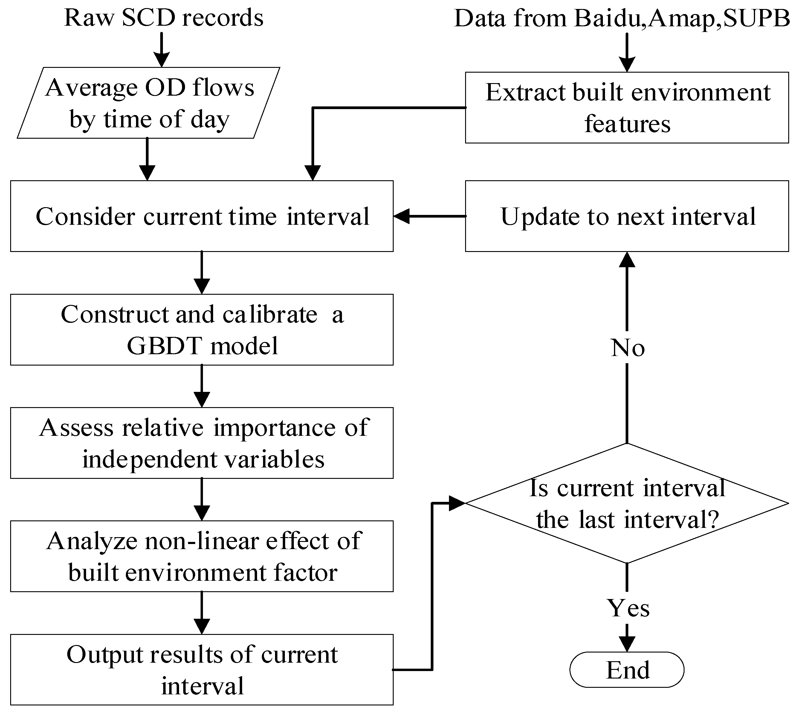
Figure 2 shows the framework of the proposed method. The framework involves three components. First, OD flows are estimated and built environment features are extracted to compile the modeling dataset. Second, for each specified time interval, a GBDT model is constructed to predict OD flows based on the built environment variables, thereby establishing the built environment–OD flow relationship. Finally, a systematic analysis is conducted focusing on two critical aspects: (1) assessing the variables’ relative importance to identify key determinants, and (2) examining the non-linear effects of built environment variables.

3.2. Modelling Approach

This study employs a GBDT model to establish a correlation between OD flow and built environment variables. Originally developed by Friedman (2001) [36], GBDT iteratively constructs weak learners (decision trees) and integrates their predictions through additive modeling, combining ensemble learning principles with decision trees. The advantages of this model include (1) mitigating multicollinearity issues, (2) identifying significant predictor variables through feature importance metrics, and (3) capturing complex non-linear relationships. It has gained popularity in contemporary transportation research, particularly in spatial–temporal mobility pattern analysis [20,37,38].
Let y denote the OD flow volume during a specific time interval. The independent variable x comprises built environment features of both the corresponding origin and destination stations. A function f(x) is constructed to approximate the response variable y based on predictor variables x. The function is initialized with a base learner (typically a constant prediction f 0 x = a r g m i n c i = 1 N L ( y i , c ) ) (c is a constant value), and then updated by minimizing the expected value of a squared-error loss function L ( y , f x ) = ( y f x ) 2 . Based on the gradient descent direction, an additive model with m regression trees is utilized to update f(x) as follows:
f m x = f m 1 x +   β m h ( x , c m )
β m = a r g   m i n i = 1 N L ( y i , f m 1 x i + β h ( x i , c ) )
where c m is the output value (leaf weight) of each terminal node in the mth regression tree h ( x , c m ) , and β m is the step size for gradient descent in model iteration, determined by minimizing the loss function.
To mitigate model overfitting, a shrinkage parameter ε   ( 0 < ε 1 ) , also referred to as the learning rate, is integrated into the function update process. This parameter scales the contribution of each tree during the additive model expansion. The modified formulation of Equation (3) can be expressed as follows:
f m x = f m 1 x +   ε β m h ( x , c m )
The gradient boosting procedure yields the ultimate model when the convergence criterion (achieving desired accuracy) or the maximum iterations is reached. The final model can be described as follows:
f x = m = 1 M γ m h ( x , c m ) ) = m = 1 M j = 1 J γ m c j m I ( x R j m )
where M is the number of decision trees (i.e., iterations), and h ( x , c m ) and γ m are the estimated result and weight of the mth tree, respectively. J is the number of leaves for each tree, x R j m = 1 ,   i f   x R j m 0 ,   o t h e r w i s e ,   and   c j m is the constant value of the corresponding region R j m (i.e., leaf j in the mth decision tree).
The relative importance of each independent variable in predicting the dependent variable can be quantified after model calibration. For a boosted ensemble, the importance score of variable x i can be computed as follows:
I x i 2 = 1 M m = 1 M I x i 2 T m I x i 2 T m = j = 1 J 1 d j
where T m is the mth decision tree, j is the number of internal nodes, and d j represents the improvement in squared error attributable to splitting on x i at the jth node. The relative importance is normalized such that their sum across all predictors equals 100%.
The partial dependence plot (PDP) [39] is employed as a visualization tool to illustrate the marginal effect of one or more predictors ( x S ) on the GBDT model’s outcomes (e.g., OD flows), while holding other variables constant. Its mathematical formulation can be expressed as follows:
f ¯ s x S = 1 N i = 1 N f ( x S , x C ( i ) )
where x S is the target predictor (e.g., pop density), x C ( i ) represents other variables, f is the prediction function of the GBDT model, and N is the sample size of dependent variables. For each value of variable x S , the model must generate predictions across all N instances of the dependent variables to compute the marginal effect.

4. Results and Discussion

4.1. Model Training and Evaluation

OD flows and their corresponding independent variables were utilized as sample data in the modelling process. Three time periods were analyzed: morning peak (7:00–9:00), midday off-peak (11:00–13:00), and afternoon peak (16:30–18:30). For each period, a GBDT model was constructed through a five-fold cross-validation, where the sample was randomly partitioned into five subsets. During each iteration, the model was trained on 80% of the data (four subsets) and validated on the remaining 20% (one subset), ensuring robust performance evaluation across all subsets.
Three key parameters of the model, namely the number of decision trees, learning rate, and maximum tree depth, were optimized using Bayesian optimization techniques [40]. Unlike the grid search approaches, this approach adaptively balances exploration and exploitation, thereby reducing computational costs and avoiding local optima. The search space was defined with the number of decision trees ranging from 200 to 1000, maximum tree depth between 4 and 8, while the learning rate was constrained to two discrete values (0.01 or 0.02). The optimal parameters can be identified, and then enable model fitting.
Model parameters and evaluation results are presented in Table 2. It is observed that the number of trees and maximum tree depth vary with time periods, while the learning rate remains constant. Model performance was evaluated using three statistical indicators: mean absolute error (MAE), mean squared error (MSE), and root mean squared error (RMSE) between observed and predicted OD flows. As indicated in Table 2, the MAEs at all periods remain below five passengers, demonstrating the models’ predictive accuracy. Notably, these indicators during midday off-peak show lower values compared to other periods, likely because peak-hour OD flows exhibit greater volatility that is more challenging for models to capture. Furthermore, the pseudo-R2 values of all models exceed 0.85, confirming strong model fit and explanatory power of the independent variables. Thus, subsequent analysis can proceed by assessing independent variables’ relative importance and generating partial dependence plots using the validated models.

4.2. Contributions of Independent Variables

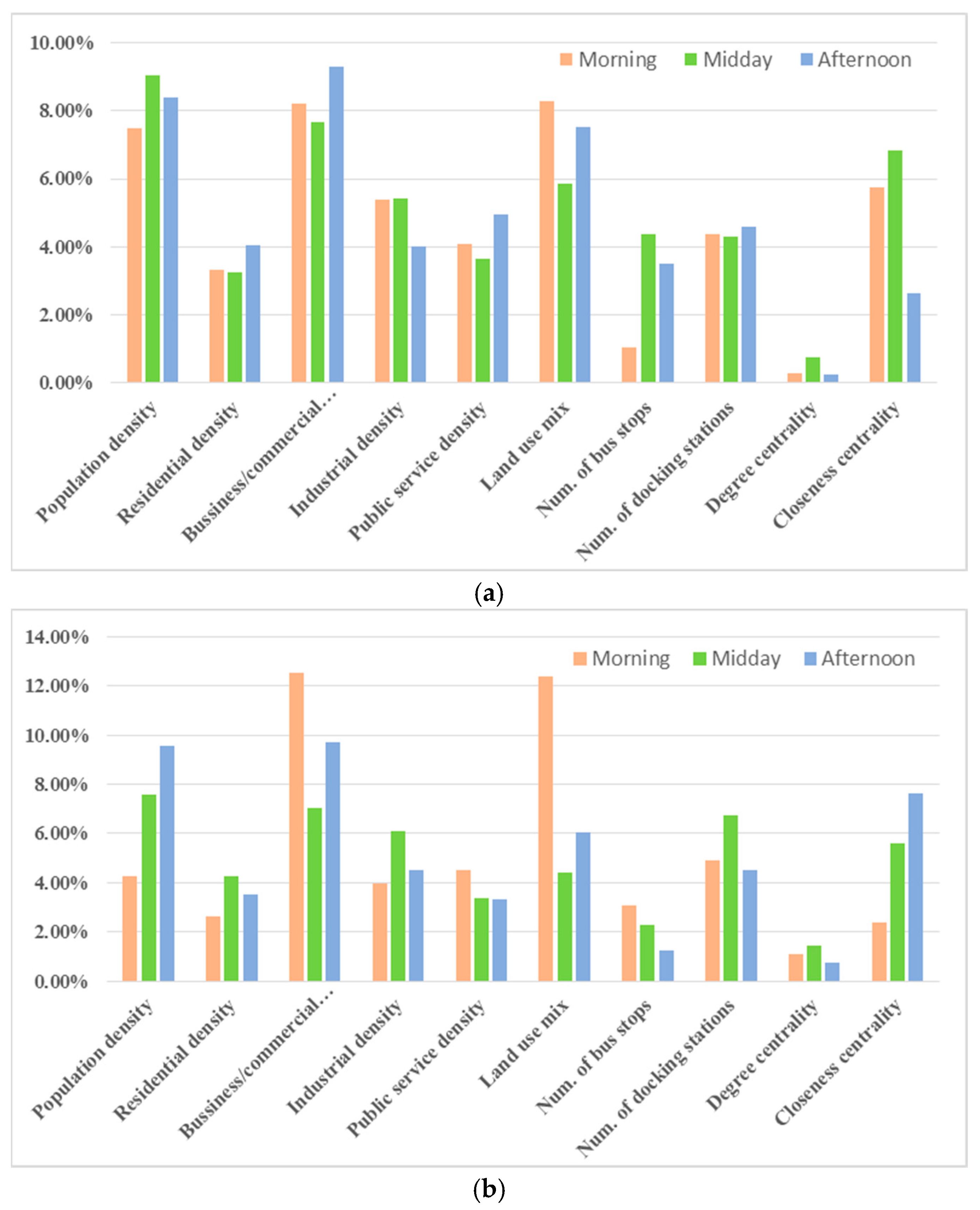
The relative importance of independent variables at three time periods is presented in Figure 3. Temporal variations in the determinants of OD flows can obviously be observed. During morning peak, business/commercial density and land use mix on both origin and destination sides are the top four most influential variables, with each contributing over 8%. Population density and closeness centrality on the origin side also have notable effects, with contributions more than 5.7%. The main contributing factors for midday off-peak are distinct. Population density and business/commercial density on both sides, combining with origin-side closeness centrality, form the top five explanatory variables (collectively contribute 38.2%). For the afternoon peak, population density and business/commercial density on both sides remain the four most important explanatory variables, but destination-side closeness centrality (7.6%) becomes the fifth most influential factor, differing from that in the other two periods.
Among the four land use factors, business/commercial density on both sides exhibits the most pronounced influence throughout all periods, with the relative importance ranging from 7 to 12.5%, whereas industrial density and public service show more modest impacts, hovering around 4%. Notably, residential density has the least impact (<4%) compared to other land use types. This finding is counterintuitive but consistent with the results from previous studies [1,25]. The reason may be that the number of residential POIs does not proportionally reflect population distribution, as residential complexes in China vary significantly in scale. Moreover, land use mix demonstrates relatively larger contributions during peak hours, particularly the morning peak on the destination side (>12%), indicating its nontrivial impact on metro ODs.
Analysis of public transit design factors reveals distinct modal preferences in Suzhou. The number of bike-sharing docking stations shows a consistent influence (approximately 4% at most periods), with a notable exception at midday off-peak on the destination side (6.7%). In contrast, the number of bus stops exhibits weaker associations (<4% in most cases), suggesting bicycle-sharing is a much popular feeder mode for metro stations. Regarding station centrality, closeness centrality demonstrates substantially higher importance on the origin side during morning peak and midday off-peak compared to the afternoon peak, but this pattern is inverted on the destination side. Degree centrality has the smallest influence among all independent variables (<1.5%), indicating that station type (whether a transfer station or not) does not constitute a critical determinant of OD prediction, though it may affect transfer flows.
A quick calculation reveals that the aggregate relative importance of independent variables is higher on the destination side for the peak hours (morning peak: 48% vs. 52%; afternoon peak: 49% vs. 51%). This implies that the destination-side built environment contributes more to peak-hour OD flow generation. However, this directional disparity diminishes to less than 2% during midday off-peak.

4.3. Non-Linear Effects of Built Environment

To explore the non-linear effects of the built environment on OD flows, the top six variables were selected based on their aggregated contributions on both sides over all time periods, ensuring the analysis focuses on the most influential factors (i.e., business/commercial density, population density, land use mix, closeness centrality, industrial density, number of bike-sharing docking stations). Then, the marginal effect of each selected variable was visualized using the partial dependence plots derived by the GBDT models.
Figure 4 depicts the effects of population density on OD flows for three time periods, with all other variables held constant. All the plots illustrate a non-linear relationship between population density and OD flows. In general, population density on both sides has a positive effect, regardless of time periods. For the peak period, taking population density on the destination side as an example, it demonstrates a positive association between population density and OD flows when the density value remains below 4000 persons/km2. However, when population density surpasses this threshold, its effect becomes negligible, as evidenced by the slight OD flow variations. Similar trends can be found at midday off-peak on either side (Figure 4b,e). Furthermore, all figures reveal that when population density exceeds 6000 persons/km2, the curves remain stable and even decline (Figure 4e,f), demonstrating a clear threshold effect on OD flows. Certain figures (Figure 4b–d) present a negative correlation within the 1300–1480 persons/km2 density range. This anomalous pattern likely stems from data outliers, as only eight stations fall within this specific interval.
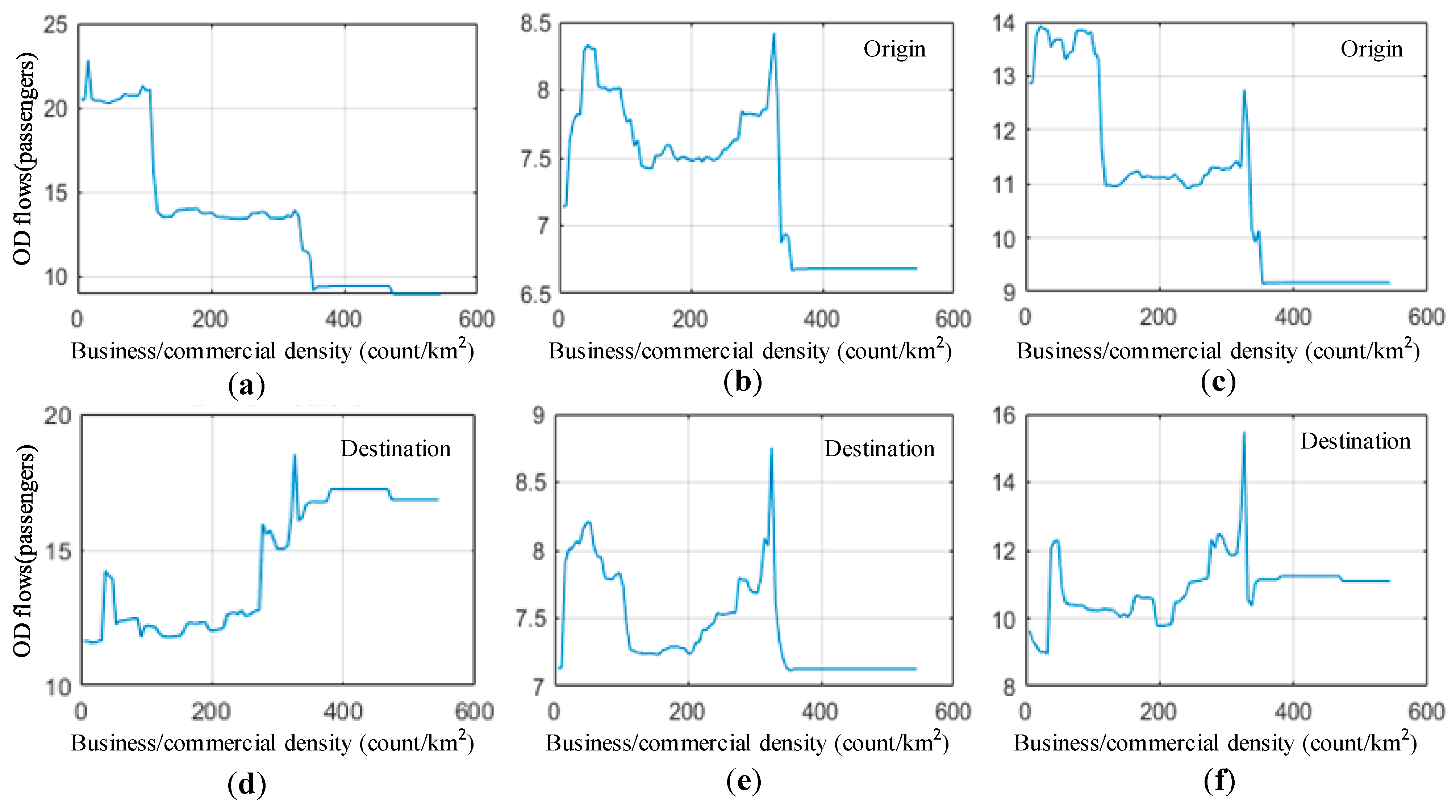
The PDPs for business/commercial density are presented in Figure 5. One can observe that business/commercial density on the origin side is negatively correlated with OD flows during the morning peak but positively associated with OD flows on the destination side. Specifically, an approximately piecewise linear relationship between origin-side business/commercial density and morning peak OD flows can be found in Figure 4a. Business/commercial density has a linear effect on OD flows when it ranges from 108 to 124, and 325 to 360 counts/km2; while in other intervals, the curve becomes horizontal, indicating a negligible effect. During the midday off-peak, the curves show strong volatility on both the origin and destination sides. Business/commercial density has a positive impact when it falls within the intervals [0, 40] and [200, 325] counts/km2. However, when it exceeds 325 counts/km2, the OD flow suddenly declines and stabilizes upon reaching 355 counts/km2. Comparative analysis of morning and afternoon peak indicates that lower business/commercial density on the origin side generates more OD flows, while during the morning peak, higher destination-side density attracts more flows; however, destination-side OD flows during the afternoon peak appear unaffected by density variations. Moreover, except for the morning peak on the origin side, business/commercial density demonstrates a threshold effect around 325 counts/km2 across all scenarios, beyond which it presents a negative impact.
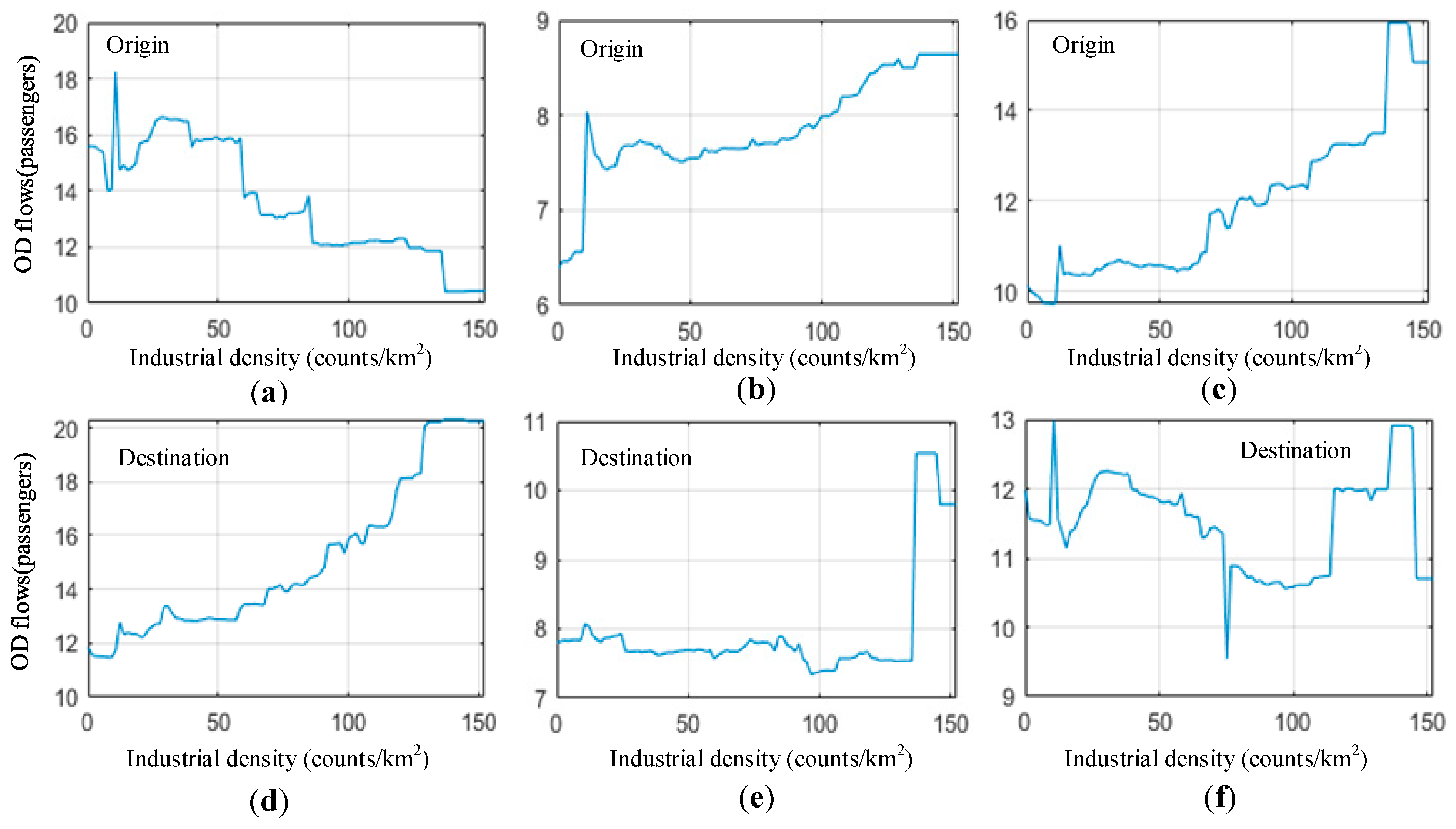
Figure 6 reveals that origin-side industrial density shows a clear negative correlation with OD flow generation, while destination-side industrial density presents a positive association with passenger attraction during the morning peak. During the afternoon peak, the relationship between industrial density and OD flows has a diametrically opposed pattern compared to the morning peak. This phenomenon aligns with real-world observations, that during the morning peak, numerous residents commute to industrial zones on the city outskirts, while evening peak flows reverse direction as workers return home or travel to commercial areas for shopping. Comparatively, OD values at midday off-peak fluctuate within a narrow range (around eight passengers) on both the origin and destination sides, indicating minimal correlation between industrial density and OD flows.
Figure 7 displays the non-linear effects of land use mix on OD flows. Overall, a threshold effect can be observed across all time periods. When the entropy value is below 0.6, the curves remain nearly flat, and only when exceeding this critical value does a clear correlation emerge. Further observation reveals similarities between the curves of the morning peak’s origin side and the evening peak’s destination side. When land use entropy values range between 0.65 and 0.7, OD values remain at a high level before suddenly declining, with the effects diminishing when the entropy exceeds 0.7. This phenomenon is basically consistent with the findings of Ding et al. [22], which suggested that land use mix should reach at least 0.6 to be the most effective. However, unlike prior studies that merely examined the relationship between the built environment and ridership, one can further observe more details on the effects of land use mix during distinct time periods in this research. As shown in Figure 7c,d, the curves of morning peak’s destination side and the evening peak’s origin side have similar trends, both demonstrating positive correlations when the entropy exceeds 0.8. This symmetry between morning-generated/evening-attracted flows (or morning-attracted/evening-generated flows) precisely mirrors the directional passenger flow patterns observed in Suzhou. During off-peak hours, while a certain degree of positive correlation emerges when the entropy exceeds 0.8, the fluctuation range of OD values remains limited. Moreover, since the origins of morning peak commuters and destinations of afternoon peak commuters in Suzhou are primarily located in residential areas, the above analysis suggests that the land use mix of the stations close to residential areas should be maintained within a reasonable range (0.65–0.7). Meanwhile, higher entropy in other areas, such as CBDs, is beneficial for enhancing peak-hour passenger demand.
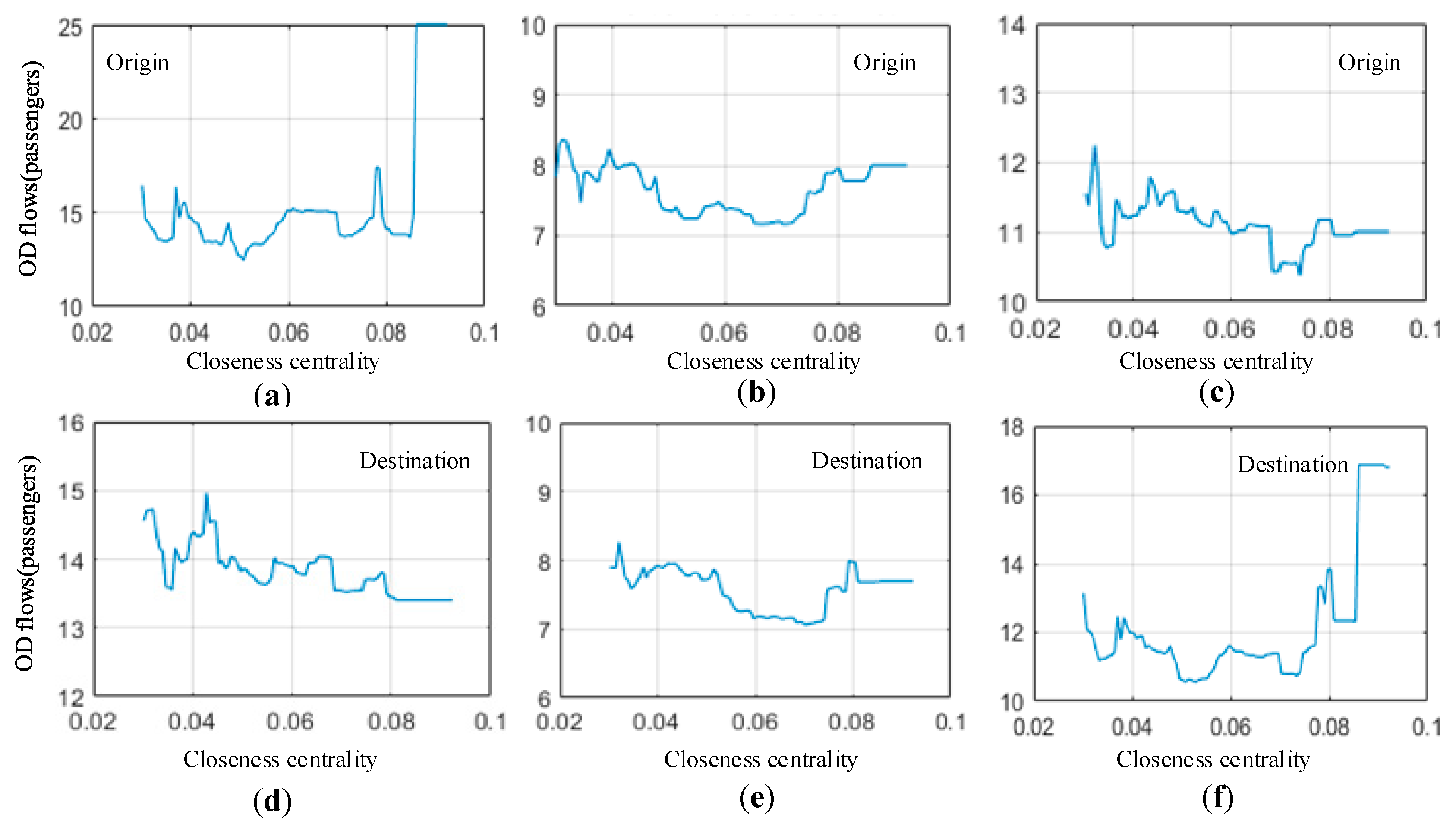
The PDPs for closeness centrality are shown in Figure 8. Figure 8a depicts that closeness centrality on the origin side has minimal impact on morning peak OD flows when it is below 0.85, with OD values fluctuating around 15 passengers. The reason may be that merely three stations’ closeness centrality values are above 0.85. While these stations are located near sub-centers, they also serve densely populated residential catchment areas. A similar pattern can be found in Figure 8f, indicating closeness centrality on the destination side also has a weak impact on afternoon peak OD flows. As shown in Figure 8b–e, a negative correlation emerges when closeness centrality values fall below 0.07, whereas a positive correlation is observed within the [0.07, 0.08] range. However, the vertical axis reveals that OD values just fluctuate within a narrow range of 1.5 passengers, indicating the slight influence of closeness centrality. This finding aligns with empirical evidence that the passenger flows in the Suzhou metro lack significant centripetal patterns across all time periods. Overall, closeness centrality demonstrates limited effects on OD flows, which further corroborates the decentralized nature of the network’s travel behavior.
Figure 9 presents the effects of the number of bike-sharing docking stations. Figure 9a–c demonstrate that on the origin side, the correlation between the number of bike-sharing docking stations and OD flows varies across different periods. For the morning peak, a positive association exists when the docking station number is below 9, but this relationship turns negative when the number ranges from 9 to 17, after which the curve flattens and the effect becomes negligible. In contrast, during midday and afternoon peak, a negative correlation is observed when the station numbers are below 6 (the reason for this remains unexplained). A similar pattern appears on the destination side during morning peak (Figure 9d). Nevertheless, Figure 9e,f show stepwise rising curves, indicating positive correlations between destination-side docking stations and OD flows. Comparing Figure 9a and f reveals that more passengers prefer bike-sharing for last-mile connections at origin stations during morning peak and at destination stations during afternoon peaks. Given residents’ commuting patterns in Suzhou, such stations are likely situated in areas with high residential land use proportions. Therefore, it is recommended to increase bike-sharing station numbers within these metro station catchment areas to an optimal count (possibly nine units, as suggested by Figure 9a,f) to attract more passengers.

5. Discussion

The proposed model examines time-varying, non-linear effects of the built environment across distinct time periods, and addresses previously ignored asymmetries by analyzing the effects on both origin and destination sides, rather than focusing solely on station ridership. It can offer practical implications for public transit and mobility planning through the implementation of its findings. There are two potential application scenarios. (1) Metro planning. By incorporating the relative importance and non-linear effects of built environments, OD flow forecasting models can prioritize contributive variables, thereby enhancing prediction accuracy. This forecasting serves as a foundation for determining critical design parameters during metro planning, including route alignment, station location/layout, and service capacity. (2) Station-area development. The non-linear relationships between built environment factors (e.g., land use density) and OD flow can inform differential zoning policies and mixed-use development strategies. For example, optimizing public transport accessibility and transit-oriented design (TOD) in station areas could mitigate uneven flow distribution and improve operational efficiency.
There are also some limitations to the proposed method. First, some critical built environment factors, such as station walkability and transit-friendliness indicators, are omitted. Second, the model framework is global and fails to capture spatial heterogeneities in built environment impacts. Finally, the variable interdependencies remain unexplored, and sensitivity analysis is absent, leaving robustness unverified.

6. Conclusions

This paper proposed a novel method for exploring the non-linear effects of station-area built environment on OD flow in a large-scale urban metro network with multiple centers. The proposed method consists of three components. First, hourly OD flows and ten kinds of built environment features were extracted as the dependent and independent variables for modeling, respectively. Second, for each specified time period (e.g., morning peak), a GBDT model was constructed to predict OD flows based on the built environment variables. Finally, the contributions of built environment variables to time-varying OD flows were assessed by calculating the relative importance, and then the non-linear effects of these variables on OD flows on both the origin and destination sides were explored using the partial dependence plots.
The proposed method was implemented on a real-world metro network in Suzhou, China. First, evaluation results showed that the GBDT models were well calibrated and fit well with the observed OD flows. Second, the contributions of built environment variables vary with time periods. Business/commercial density and land use mix on both sides are the top four most influential variables for morning peak, while population density and business/commercial density on both sides form the top four explanatory variables for midday off-peak and afternoon peak. Third, most independent variables have time-varying, discontinuous, non-linear effects on OD flows, and some variables show threshold effects on OD flows (e.g., population density with a threshold of 6000 persons/km2). Even for the same variable, its non-linear effects demonstrate notable differences between the origin and destination sides. Third, among the two variables related to public transit design, the number of shared-bicycle docking stations shows a higher contribution to OD flows than the number of bus stops. It has a positive effect on morning peak OD generation at origins and afternoon peak OD attraction at destinations, with a threshold effect below nine counts. Last, this research also reveals novel findings that appear counterintuitive but are explainable including, (a) residential density exerts the least impact among all land use types; (b) the number of bike-sharing docking stations is a more important variable than the number of bus stops in Suzhou network; (c) a higher degree of land-use balance does not always correlate with improved OD demands, and the land use mix of the stations close to residential areas should be maintained within a reasonable range (0.65–0.70).
Even though the proposed method achieved satisfactory outcomes, several further research directions can be taken to expand this work. First, only the built environment features were considered to construct the OD prediction model. The OD flows are also affected by factors such as social status, walking access to the metro station [41,42], transit fares, trip length, and commuter details. These variables could be used as new inputs to enhance the proposed model. Second, the proposed method may be further integrated with geographically weighted approaches to explore spatial heterogeneity in the relationship between passenger flow and independent variables. Lastly, the interaction effects among multiple variables could be explored in the future.

Author Contributions

Conceptualization, W.R.; methodology, W.R. and S.K.; software, Y.Y.; validation, S.K. and Y.Y.; formal analysis, Y.Y.; investigation, W.R.; resources, Z.L.; data curation, Y.Y.; writing—original draft preparation, W.R.; writing—review and editing, S.K.; visualization, Y.Y.; supervision, Z.L.; project administration, W.R.; funding acquisition, W.R. and Z.L. All authors have read and agreed to the published version of the manuscript.

Funding

This research was funded by ‘The Humanities and Social Science Fund of the Ministry of Education of China, grant number 24YJCZH237’, ‘The Industry-University-Research Collaboration Project of Jiangsu province, grant number BY20240208’, and ‘The Natural Science Foundation of the Jiangsu Higher Education Institutions of China, grant number 23KJB580008’.

Institutional Review Board Statement

Not applicable.

Informed Consent Statement

Not applicable.

Data Availability Statement

The data can be made available upon request.

Conflicts of Interest

The authors declare no conflicts of interest.

References

  1. Zhao, J.; Deng, W.; Song, Y. Analysis of metro ridership at station level and station-to-station level in Nanjing: An approach based on direct demand models. Transportation 2014, 41, 133–155. [Google Scholar] [CrossRef]
  2. Durning, M.; Townsend, C. Direct Ridership Model of Rail Rapid Transit Systems in Canada. Transp. Res. Rec. J. Transp. Res. Board 2015, 2537, 96–102. [Google Scholar] [CrossRef]
  3. Estupinan, N.; Rodriguez, D.A. The relationship between urban form and station boardings for Bogota’s BRT. Transp. Res. Part A Policy Pract. 2008, 42, 296–306. [Google Scholar] [CrossRef]
  4. Gutierrez, J.; Cardozo, O.; Garcia-Palomares, J. Transit ridership forecasting at station level: An approach based on distance-decay weighted regression. J. Transp. Geogr. 2011, 19, 1081–1092. [Google Scholar] [CrossRef]
  5. Choi, J.; Lee, Y.; Kim, T. An analysis of metro ridership at the station-to-station level in Seoul. Transportation 2012, 39, 705–722. [Google Scholar] [CrossRef]
  6. Thompson, G.; Brown, J.; Bhattacharya, T. What really matters for increasing transit ridership: Understanding the determinants of transit ridership demand in Broward County, Florida. Urban Stud. 2012, 49, 3327–3345. [Google Scholar] [CrossRef]
  7. Li, S.; Lyu, D.; Liu, X. The varying patterns of rail transit ridership and their relationships with fine-scale built environment factors: Big data analytics from Guangzhou. Cities 2020, 99, 102580. [Google Scholar] [CrossRef]
  8. Chen, W.; Chen, X.; Chen, J. What factors influence ridership of station-based bike sharing and free-floating bike sharing at rail transit stations? Inter. J. Sustain. Transp. 2022, 16, 357–373. [Google Scholar] [CrossRef]
  9. Peng, J.; Fu, X.; Wu, C.; Dai, Q.; Yang, H. Comparative analysis of nonlinear impacts on the built environment within station areas with different metro ridership segments. Travel Behav. Soc. 2025, 38, 100898. [Google Scholar] [CrossRef]
  10. Cordera, R.; Coppola, P.; dell’Olio, L.; Ibeas, Á. Is accessibility relevant in trip generation? Modelling the interaction between trip generation and accessibility taking into account spatial effects. Transportation 2017, 44, 1577–1603. [Google Scholar] [CrossRef]
  11. Ewing, R.; Cervero, R. Travel and the built environment. J. Amer. Plan. Assoc. 2010, 76, 265–294. [Google Scholar] [CrossRef]
  12. Cardozo, O.; García-Palomares, J.; Gutiérrez, J. Application of geographically weighted regression to the direct forecasting of transit ridership at station-level. App. Geogr. 2012, 34, 548–558. [Google Scholar] [CrossRef]
  13. Sung, H.; Choi, K.; Lee, S. Exploring the impacts of land use by service coverage and station-level accessibility on rail transit ridership. J. Transp. Geogr. 2014, 36, 134–140. [Google Scholar] [CrossRef]
  14. Zhu, Y.; Chen, F.; Wang, Z. Spatio-temporal analysis of rail station ridership determinants in the built environment. Transportation 2019, 46, 2269–2289. [Google Scholar] [CrossRef]
  15. Jun, M.; Choi, K.; Jeong, J.; Kwon, K.; Kim, H. Land use characteristics of subway catchment areas and their influence on subway ridership in Seoul. J. Transp. Geogr. 2015, 48, 30–40. [Google Scholar] [CrossRef]
  16. Yu, H.; Peng, Z. Exploring the spatial variation of ridesourcing demand and its relationship to built environment and socioeconomic factors with the geographically weighted Poisson regression. J. Transp. Geogr. 2019, 75, 147–163. [Google Scholar] [CrossRef]
  17. Shi, Z.; Zhang, N.; Liu, Y. Exploring spatiotemporal variation in hourly metro ridership at station level: The influence of built environment and topological structure. Sustainability 2018, 10, 4564. [Google Scholar] [CrossRef]
  18. Liu, X.; Wu, J.; Huang, J. Spatial-interaction network analysis of built environmental influence on daily public transport demand. J. Transp. Geogr. 2021, 92, 102991. [Google Scholar] [CrossRef]
  19. van Wee, B.; Handy, S. Key research themes on urban space, scale, and sustainable urban mobility. Int. J. Sustain. Transp. 2016, 10, 18–24. [Google Scholar] [CrossRef]
  20. Ding, C.; Cao, X.; Næss, P. Applying gradient boosting decision trees to examine non-linear effects of the built environment on driving distance in Oslo. Transp. Res. Part A Policy Pract. 2018, 110, 107–117. [Google Scholar] [CrossRef]
  21. Shen, Y.; Zhang, L.; Song, Y.; Wang, C.; Yu, Z. Nonlinear influence of urban environment on dockless shared bicycle travel patterns. Sustainability 2025, 17, 4575. [Google Scholar] [CrossRef]
  22. Ding, C.; Cao, X.; Liu, C. How does the station-area built environment influence Metrorail ridership? Using gradient boosting decision trees to identify non-linear thresholds. J. Transp. Geogr. 2019, 77, 70–78. [Google Scholar] [CrossRef]
  23. Liu, X.; Chen, X.; Tian, M. Effects of built environment on metro ridership considering stage of growth. J. Transp. Syst. Eng. Inf. Technol. 2023, 23, 121–127. [Google Scholar]
  24. Du, Q.; Zhou, Y.; Huang, Y. Spatiotemporal exploration of the non-linear impacts of accessibility on metro ridership. J. Transp. Geogr. 2022, 102, 103380. [Google Scholar] [CrossRef]
  25. Li, P.; Chen, X.; Lu, W. Research on nonlinear relationship between subway built environment and travel distance of stations based on XGBoost-SHAP. J. Railw. Sci. Eng. 2024, 21, 1624–1633. [Google Scholar]
  26. Li, P.; Yang, Q.; Lu, W.; Xi, S.; Wang, H. An improved machine learning framework considering spatiotemporal heterogeneity for analyzing the relationship between subway station-level passenger flow resilience and land use-related built environment. Land 2024, 13, 1887. [Google Scholar] [CrossRef]
  27. Pang, L.; Ren, L.; Jiang, Y.; Yun, Y. Mechanism of impact of the built environment of urban rail transit origin and destination stations on network ridership during peak hours. Prog. Geogr. 2024, 43, 1785–1797. [Google Scholar]
  28. Gan, Z.; Yang, M.; Feng, T.; Timmermans, H. Examining the relationship between built environment and metro ridership at station-to-station level. Transp. Res. Part D. Transp. Environ. 2020, 82, 102332. [Google Scholar] [CrossRef]
  29. Liu, B.; Xu, Y.; Guo, S. Examining the nonlinear impacts of origin-destination built environment on metro ridership at station-to-station level. Inter. J. Geo-Inform. 2023, 12, 59. [Google Scholar] [CrossRef]
  30. The Website of Suzhou Municipal Transport Bureau. Available online: http://jtj.suzhou.gov.cn/szjt/xwfbmtjj/202302/43216ef0f3414deab37f86df42314b4f.shtml (accessed on 9 February 2023).
  31. Shannon, C.; Weaver, W. The Mathematical Theory of Communication; University of Illinois Press: Urbana, IL, USA, 1949. [Google Scholar]
  32. Cervero, R.; Kockelman, K. Travel demand and the 3Ds: Density, diversity, and design. Transp. Res. Part D Transp. Environ. 1997, 2, 199–219. [Google Scholar] [CrossRef]
  33. Liu, R.; Xu, J.; Iris, C.; Chen, J. Dynamic rebalancing strategies for dockless bike-sharing systems. Inter. J. Prod. Econ 2025, 285, 109634. [Google Scholar] [CrossRef]
  34. Basak, E.; Iris, Ç. Urban Life Matters: The Heterogeneous Effects of On-Demand Bike Sharing Platforms on Urban Transit. 2023. Available online: https://papers.ssrn.com/sol3/papers.cfm?abstract_id=4391093 (accessed on 29 March 2023).
  35. Arentze, T.; Timmermans, H. A learning-based transportation oriented simulation system. Transp. Res. Part B Methodol. 2004, 38, 613–633. [Google Scholar] [CrossRef]
  36. Friedman, J. Greedy function approximation: A gradient boosting machine. Ann. Stat. 2001, 29, 1189–1232. [Google Scholar] [CrossRef]
  37. Wang, W.; Wang, H.; Xu, J.; Liu, C.; Wang, S.; Miao, Q. Interpretable GBDT Model for analysing Ridership Mechanisms in Urban Rail Transit: A Case Study in Shenzhen. Appl. Sci. 2025, 15, 3835. [Google Scholar] [CrossRef]
  38. Li, L.; Huang, C.; Liu, Y. Detecting the contribution of transport development to urban construction land expansion in the Beijing-Tianjin-Hebei region of China based on machine learning. Land Use Policy 2025, 157, 107622. [Google Scholar] [CrossRef]
  39. Hastie, T.; Tibshirani, R.; Friedman, J. The Elements of Statistical Learning: Data Mining, Inference, and Prediction, 2nd ed.; Springer: Berlin/Heidelberg, Germany, 2009. [Google Scholar]
  40. Ian, D.; McCourt, M.; Clark, S. Bayesian Optimization for Machine Learning: A Practical Guidebook; SigOpt: San Francisco, CA, USA, 2024. [Google Scholar]
  41. Sun, G.; Zacharias, J.; Ma, B.; Oreskovic, N. How do metro stations integrate with walking environments? Results from walking access within three types of built environment in Beijing. Cities 2016, 56, 91–98. [Google Scholar] [CrossRef]
  42. Wehbi, L.; Bektaş, T.; Iris, Ç. Optimising vehicle and on-foot porter routing in urban logistics. Transp. Res. Part D Transp. Environ. 2022, 109, 103371. [Google Scholar] [CrossRef]
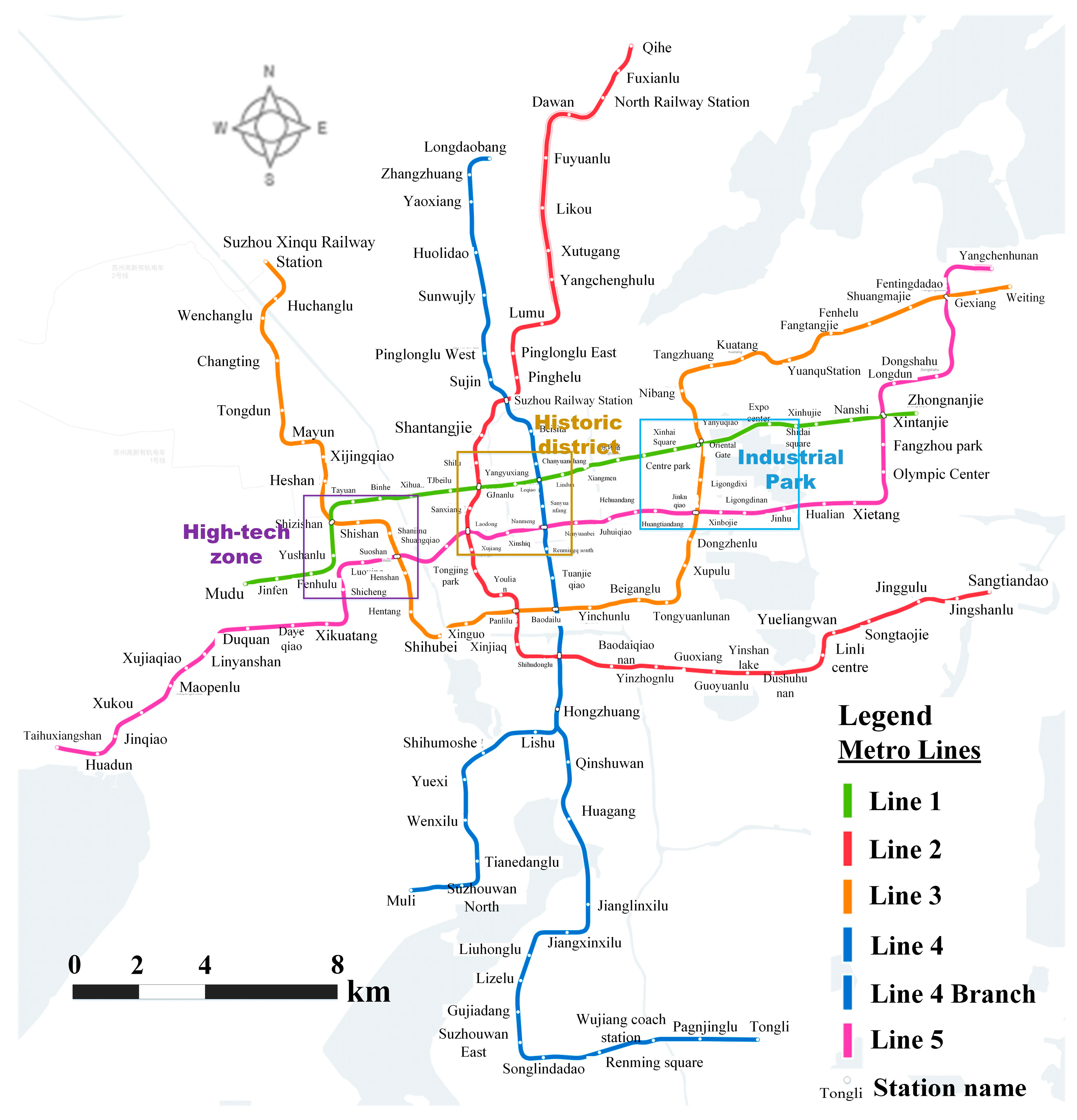
Figure 1. Study area and Suzhou metro network in 2022.
Sustainability 17 08829 g001
Figure 2. Framework of the proposed method.
Sustainability 17 08829 g002
Figure 3. Relative importance of independent variables, including (a) variables on origin side; (b) variables on destination side.
Sustainability 17 08829 g003
Figure 4. The effects of population density on OD flows, including (a) morning peak, origin side; (b) midday off-peak, origin side; (c) afternoon peak, origin side; (d) morning peak, destination side; (e) midday off-peak, destination side; (f) afternoon peak, destination side.
Sustainability 17 08829 g004
Figure 5. The effects of business/commercial density on OD flows, including (a) morning peak, origin side; (b) midday off-peak, origin side; (c) afternoon peak, origin side; (d) morning peak, destination side; (e) midday off-peak, destination side; (f) afternoon peak, destination side.
Sustainability 17 08829 g005
Figure 6. The effects of industrial density on OD flows, including (a) morning peak, origin side; (b) midday off-peak, origin side; (c) afternoon peak, origin side; (d) morning peak, destination side; (e) midday off-peak, destination side; (f) afternoon peak, destination side.
Sustainability 17 08829 g006
Figure 7. The effects of land use mix on OD flows, including (a) morning peak, origin side; (b) midday off-peak, origin side; (c) afternoon peak, origin side; (d) morning peak, destination side; (e) midday off-peak, destination side; (f) afternoon peak, destination side.
Sustainability 17 08829 g007
Figure 8. The effects of closeness centrality on OD flows, including (a) morning peak, origin side; (b) midday off-peak, origin side; (c) afternoon peak, origin side; (d) morning peak, destination side; (e) midday off-peak, destination side; (f) afternoon peak, destination side.
Sustainability 17 08829 g008
Figure 9. The effects of number of bike-sharing docking stations on OD flows, including (a) morning peak, origin side; (b) midday off-peak, origin side; (c) afternoon peak, origin side; (d) morning peak, destination side; (e) midday off-peak, destination side; (f) afternoon peak, destination side.
Sustainability 17 08829 g009
Table 1. Summary of the independent and dependent variables.
Variable NameData SourceMeanSt. Dev.
Dependent variables
OD flows
Morning peak (7:00–9:00)SMC14.0227.65
Midday off-peak (11:00–13:00)SMC7.738.28
Afternoon peak (16:30–18:30)SMC11.3016.96
Build environment characteristics
Density
Population density (persons/km2)Baidu map, SUPB27271176
Residential density (counts/km2)AMap3639
Business/commercial density(counts/km2)AMap210119
Industrial density (counts/km2)AMap5438
Public service density (counts/km2)AMap13799
Diversity
Land use mixCalculated0.790.12
Design
Number of bus stops (counts)AMap6.12.4
Number of bike-sharing docking stations (counts)AMap5.65.3
Station centrality
Degree centralityMeasured from metro network2.300.82
Closeness centralityCalculated0.0500.013
Table 2. Model parameters and evaluation results.
Time PeriodsSample SizeNumber of TreesLearning RateMaximum Tree DepthEvaluation Metrics
MAEMSERMSER2
Morning peak10,1989680.0264.9075.988.720.90
Midday off-peak53906950.0271.818.212.870.88
Afternoon peak97868670.0263.6337.896.160.87
Disclaimer/Publisher’s Note: The statements, opinions and data contained in all publications are solely those of the individual author(s) and contributor(s) and not of MDPI and/or the editor(s). MDPI and/or the editor(s) disclaim responsibility for any injury to people or property resulting from any ideas, methods, instructions or products referred to in the content.