Examining Characteristics and Causes of Juglar Cycles in China, 1981–2024

Abstract

This study provides a comprehensive empirical examination of the drivers and dynamics of Juglar cycles in China from 1981 to 2024. We develop a unified framework that integrates investment, institutional, productivity, and structural factors, and employ a Vector Error Correction Model to analyze the long-run equilibrium and short-run adjustment mechanisms linking fixed asset investment (FAI), government fiscal expenditure (GFE), total factor productivity (TFP), industrial structure upgrading (ISU), and gross domestic product (GDP). Our results confirm a stable cointegration relationship and identify FAI as the most influential long-run driver of output, with a 1% increase in FAI leading to a 0.88% rise in GDP. Industrial upgrading also exerts a positive long-run influence on growth, whereas government spending exhibits a significant negative effect, potentially indicating crowding-out or efficiency losses. In the short run, we find unidirectional Granger causality from FAI to GDP, suggesting that changes in investment contain meaningful predictive power for future output fluctuations. Furthermore, impulse response and variance decomposition analyses illustrate the temporal evolution of these effects, highlighting that the contribution of TFP gains importance over the medium term. Overall, this study deepens our understanding of business cycle transmission mechanisms in emerging economies and offers valuable insights for policymakers seeking to balance investment-driven growth with structural reforms for sustainable and robust economic development.

1. Introduction

Since the founding of the People’s Republic of China in 1949, China’s economic development has undergone a dynamic trajectory encompassing recovery, rapid growth, structural adjustment, and ultimately a transition toward high-quality development. This process has been marked by inevitable cyclical fluctuations, including phases such as post-war recovery and reconstruction (1949–1952) [1,2], the establishment of the industrial foundation under the First Five-Year Plan, and subsequent periods of fluctuation and adjustment from the Great Leap Forward to the Cultural Revolution [3,4,5,6,7,8,9]. A major turning point occurred with the reform and opening-up policy, initiated at the Third Plenary Session of the Eleventh Central Committee in 1978 [10,11]. Reforms began in rural areas with the household contract responsibility system, which substantially increased agricultural productivity by enhancing farmers’ incentives. These were followed by urban reforms aimed at restructuring state-owned enterprises and promoting the growth of private businesses, thereby fostering economic diversification. The establishment of Special Economic Zones and coastal open cities further accelerated the inflow of foreign capital and technology, accelerating trade expansion [12,13,14,15,16]. As a result, China witnessed remarkable economic growth, with gross domestic product (GDP) rising at an average annual rate of approximately 9% between 1978 and 1992. The economy also underwent structural transformation: industry and services grew as a share of output, while agriculture’s share declined. This period also included episodes of volatility, such as the economic overheating of 1984–1985, which featured elevated investment and inflation [17,18,19]. Macro-control policies—including credit tightening and price controls—were implemented to stabilize economic conditions. The 14th National Congress of the Communist Party of China officially endorsed the goal of building a socialist market economy, paving the way for deeper market-oriented reforms in fiscal and financial systems. Shareholding reforms in state-owned enterprises were also advanced, enhancing market efficiency and dynamism [20]. Between 1992 and 2008, GDP grew at an average rate exceeding 10% annually. China’s accession to the World Trade Organization (WTO) further accelerated foreign trade and investment, solidifying its position as a global manufacturing and trading hub. During this period, infrastructure improved markedly, and technological progress became an increasingly important driver of productivity growth [21].

Despite these achievements, China’s development path has been punctuated by significant challenges and cyclical fluctuations. The 1997 Asian Financial Crisis slowed China’s growth through shrinking exports, prompting a policy response that combined expansionary fiscal measures with prudent monetary policy to sustain domestic demand and stabilize the economy [22,23]. Similarly, the 2008 Global Financial Crisis triggered a sharp decline in external demand, leading to falling exports and reduced corporate orders [24]. In response, China implemented a massive stimulus package—the Four-Trillion-Yuan Plan—focused on infrastructure investment and consumption subsidies to help maintain macroeconomic stability. Thereafter, China’s economy subsequently entered a new normal phase, transitioning from high-speed to medium–high growth with structural reform and upgrading emerging as key priorities. Supply-side policies were designed to cut overcapacity, reduce leverage, lower costs, and address structural weaknesses, aiming to establish a more sustainable growth model [25,26]. As the world’s second-largest economy, largest trading nation, and a systemic global player, China’s economic fluctuations exert far-reaching spillover effects. These cycles transmit growth, inflation, and instability worldwide, while also generating significant opportunities. Underestimating these dynamics could lead to miscalibrations in market forecasts, policy design, and geopolitical strategies, making it essential to closely monitor China’s economic pulse. Therefore, analyzing the characteristics and drivers of China’s economic cycles carries both academic and practical significance—particularly amid growing international scrutiny regarding the sustainability of its investment-driven growth model [27].

While Juglar cycle theory emphasizes credit-driven investment fluctuations, its core essence lies in explaining medium-term cycles through periodic waves of fixed asset investment (FAI). China’s unique institutional context, however, has reconfigured the underlying drivers of such investment cycle. In China, state-led resource mobilization—expressed through government fiscal policies, industrial policies that guide upgrading, and productivity targets—often serves as the primary catalyst for investment surges, serving a function analogous to credit booms in market economies. Therefore, analyzing China’s Juglar cycle through the interplay of government fiscal expenditure (GFE), FAI, total factor productivity (TFP), and industrial structure upgrading (ISU) does not deviate from but rather contextualizes the theory’s modern manifestation within a state-influenced financial system.

The trajectory of China’s economic development has exhibited clear cyclical patterns, prompting substantial academic interest in the presence and persistence of Juglar cycles within its growth model. Recent policy developments have further highlighted the relevance of this framework. In 2024, China’s Central Financial and Economic Affairs Commission announced an ambitious three-trillion-yuan initiative to support large-scale equipment renewal and technological transformation of production facilities over the next five years. This substantial investment commitment, together with policies promoting consumer goods replacement and lower logistics costs, signals a potential new phase of cyclical upswing in China’s Juglar cycle. Against this backdrop, there is a compelling rationale for analyzing the structural relationships among investment, productivity, institutional factors, and economic output within China’s unique economic transition context.

While extensive research exists on China’s economic growth, several significant gaps remain in understanding the specific mechanisms through which Juglar cycles manifest in the Chinese context. First, there is insufficient empirical investigation examining the combined influence of multiple cycle drivers—FAI, government fiscal policies, TFP, and ISU. Second, existing studies often fail to account for the time-varying nature of these relationships as China’s economy has undergone fundamental structural transformations. Third, there is limited research employing econometric frameworks capable of distinguishing both short-term dynamics and long-term equilibrium relationships among these variables.

Our study contributes to the existing literature in several important ways. First, we provide a comprehensive empirical examination of Juglar cycle drivers in China that simultaneously incorporates investment, institutional, productivity, and structural factors. Second, we identify distinct temporal patterns in these relationships, offering new insights into how China’s economic cycles have evolved alongside institutional reforms and development stage transitions. Third, we present empirical evidence regarding the changing effectiveness of investment-driven growth models as China’s economy matures, with important implications for policy design and implementation.

The remainder of this study is structured as follows: Section 2 reviews the relevant literature on economic cyclical fluctuations. Section 3 presents the theoretical framework and methodology. Section 4 discusses the Juglar cycle in China and its underlying causes, while Section 5 provides an empirical analysis of the relationship between GDP and FAI, along with the impact of fiscal policies, TFP, and ISU. Section 6 offers the conclusions, policy implications of the study, discusses limitations, and suggests directions for future research.

2. Literature Review

The Juglar cycle, first identified by French economist Clément Juglar in 1862, provides a classical framework for analyzing investment-driven economies, and aligns with the renewal cycles of large-scale equipment and infrastructure [28]. Although economic fluctuations occur at various frequencies, this study focuses on identifying and examining Juglar cycles within China’s post-reform economy (1981–2024) based on the following reasons: (1) Dominant driver of macroeconomic fluctuations. China’s growth has been largely investment-led, marked by high and volatile FAI, sustained by credit expansion. This aligns with the theoretical core of Juglar cycles, in which fixed investment serves as the primary driver of medium-term fluctuations—boom, overcapacity, downturn, and recovery [29,30]. Although consumption and net exports are vital components of aggregate demand and long-term growth, investment has been the dominant source of cyclical volatility in China’s development model, characterized by its high amplitude and direct link to credit cycles and policy shifts. (2) Policy relevance. Juglar-frequency fluctuations have major implications for financial risk, industrial overcapacity, employment, and growth stability. A deeper understanding of China’s Juglar cycle is essential for counter-cyclical policymaking. While the Juglar cycle offers a sound theoretical basis, empirical studies explicitly examining multi-dimensional drivers—including FAI, fiscal policy, TFP, and ISU—within China’s Juglar-cycle context remain limited.

Economic cycles reflect periodic fluctuations in aggregate output, income, and employment, typically comprising four phases: contraction, trough, expansion, and peak. Based on duration, cycles are commonly categorized into four types [31,32,33,34,35,36] (

Table 1. Types of Economic Cycles.

Cycle Name	Cycle Type	Average Length	Source of Cycle
Kitchin cycle	Short cycle	4 years (3~5 years)	Enterprise inventory investment
Juglar cycle	Medium cycle	9 years (8~10 years)	Enterprise equipment investment
Kuznets cycle	Medium-long cycle	20 years (15~25 years)	Construction investment
Kondratieff cycle	Long cycle	50 years (45~60 years)	Scientific and technological development

): Kitchin cycle (inventory cycle, 3–5 years), Juglar cycle (equipment investment cycle, 8–10 years), Kuznets cycle (construction cycle, 15–25 years), and Kondratiev cycle (technological waves, 45–60 years).

The relevance of Juglar’s theory extends far beyond its 19th-century origins and remains a potent tool for analyzing modern economic fluctuations. Compelling empirical evidence for its global applicability comes from the spectral analysis of world GDP dynamics by Korotayev and Tsirel [37], which identified statistically significant medium-term fluctuations (7–11 years) consistent with Juglar cycles, alongside shorter Kitchin and longer Kuznets and Kondratiev waves. Building on this empirical foundation, Grinin, Korotayev, and Malkov further advanced the theoretical rigor of the Juglar framework by constructing a formal mathematical model [38]. Their model explicitly links the phases of the Juglar cycle to the interplay of credit, investment, and innovation dynamics. A pivotal contribution of their work is the successful application of this model to analyze the 2008–2009 Global Financial Crisis, arguing that its patterns are fundamentally consistent with the Juglar cycle’s downturn phase. This provides a powerful, mechanism-based argument for the enduring theoretical relevance and empirical validity of Juglar’s periodization in the 21st-century global economy. These studies collectively affirm that the Juglar cycle is not a historical relic but a living analytical framework, thereby establishing a foundation for examining its specific reconfigurations within unique institutional contexts, such as China’s state-influenced economy.

In China, economic cycles stem from more than just aggregate shocks, arising instead from complex interactions among sectoral shocks, institutional reform, and production networks [39]. Notably, capital-intensive and real estate sectors amplify cyclical volatility [40,41], with state-owned enterprises (SOEs) continuing to play a significant role in shaping macroeconomic fluctuations [42]. China has exhibited improved stability, domestically driven transmission mechanisms, and high sectoral heterogeneity [43,44]. These fluctuations are shaped by production networks, policy interventions, and global integration [45]. Existing research has employed methodologies such as SVAR, DSGE, and production network models to analyze these fluctuations [46,47,48]. Recent research has employed estimated DSGE models with housing and banking sectors to identify key drivers of these cycles [49].

However, few studies adopt cointegrated multivariate frameworks capable of simultaneously analyzing investment, policy, productivity, and structural factors. This analytical shortcoming persists despite a growing recognition in the literature on emerging economies of the need to integrate multiple drivers—such as external finance, investment, and sectoral composition—to fully grasp growth dynamics, as evidenced by studies on Nigeria and Angola [50,51]. Many also neglect non-stationarity, structural breaks, and spurious regression in macroeconomic series [52,53,54,55], undermining the reliability of their inferences. This gap is especially critical given China’s transitional economy, where frequent institutional shifts and policy interventions introduce structural breaks. Although empirical studies using neoclassical models have identified investment wedges and factor market distortions as key cycle drivers [56,57], conventional modeling approaches like SVAR and DSGE remain limited in capturing China’s institutional reality. SVARs often rely on identification schemes rooted in market-economy mechanisms that are misaligned with China’s state-influenced financial system [58], while DSGE models struggle to accommodate institutional evolution and frequent policy shocks [59]. In this context, cointegration analysis and Vector Error Correction Model (VECM) offer a more robust framework, explicitly addressing non-stationarity and structural breaks while identifying long-run relationships among variables [60,61,62]. This makes them particularly suitable for analyzing China’s investment-driven medium-term cycles and capturing the policy-anchored growth dynamics underlying its economic fluctuations.

This study aims to address these research gaps by constructing a systematic analytical framework to examine China’s Juglar cycle dynamics through the following objectives: (1) analyze the long-term equilibrium relationship between FAI, GFE, TFP, ISU, and GDP growth; (2) identify the short-term adjustment mechanisms that maintain equilibrium relationships among these variables; and (3) explore the implications of these dynamics for understanding Juglar cycles in the Chinese economy.

3. Method and Model

Since macroeconomic variables such as GDP and FAI are typically non-stationary, direct regression analysis would yield spurious results. To achieve these objectives, we employ a VECM that allows us to capture both short-term dynamics and long-term equilibrium relationships among our variables of interest. This methodological approach is particularly appropriate for analyzing non-stationary time series data that share common stochastic trends—a characteristic feature of macroeconomic variables. Several techniques are used to assess cointegration in time series models.

3.1. Hodrick–Prescott Filtering Method

The HP filter, which employs symmetric weights and a moving average principle to extract a smooth trend from time series data, was first proposed by Hodrick and Prescott [63] and applied to the empirical analysis of post-war U.S. business cycles. Currently, the HP filter is widely applied to both real and simulated time series for detrending non-stationary data in applied econometrics [64]. We acknowledge its well-known limitations, primarily end-point bias and the subjective nature of the smoothing parameter (λ) selection. Following the standard practice in macroeconomics for annual data [65], we set λ = 6.25 in this study. Let $\left\{Y_t\right\}$ be the economic time series, and $\left\{Y_t^T\right\}$ and $\left\{Y_t^C\right\}$ be the trend and cycle components contained therein respectively. Then:

$$Y_t=Y_t^T+Y_t^C t=\mathrm{1,2},\dots ,T$$

(1)

If $Y_t^C$as well as the second difference of $Y_t^T$ are normally and independently distributed, then the HP filter is known to be optimal. The calculation of the HP filter is essentially to separate the trend component $\left\{Y_t^T\right\}$ from $\left\{Y_t\right\}$, which is to find the solution of the following minimization problem:

$$Min\left\{\sum _{t=1}^T{(Y_t-Y_t^T)}^2+\lambda \sum _{t=1}^T{\left(\right(Y_{t+2}^T-Y_{t+1}^T)-(Y_{t+1}^T-Y_t^T\left)\right)}^2\right\}$$

(2)

The first term of this formula measures the fluctuating component, the residual $Y_t -Y_t^T$ is referred to as the business cycle component. The second term measures the degree of smoothness of the trend term, where $(Y_{t+2}^T - Y_{t+1}^T) - (Y_{t+1}^T - Y_t^T)$ represents the second-order differences in the trend $Y_t^T$, and $\lambda$ represents the smoothing parameter, which penalizes the acceleration in the trend relative to the business cycle component. Researchers typically set $\lambda$ = 129,600, 1600 and 6.25 for monthly data, quarterly data and annual data, respectively [65]. When λ = 0, the trend sequence $\left\{Y_t^T\right\}$ coincides with the original sequence $\left\{Y_t\right\}$. As λ increases, the estimated trend becomes progressively smoother, reflecting a stronger penalty on short-term fluctuations.

3.2. Stationarity Test

This approach is necessary because autoregressive (AR) models require stationary time series. A time series is stationary if its mean and autocovariances are independent of time; otherwise, it is non-stationary. The ADF test constructs a parametric correction for higher-order correlation by assuming that the $Y$ series follows an AR(p) process and adding p lagged difference terms of the dependent variable $\mathrm{Y}$ to the right-hand side of the test regression:

$${∆Y}_t=(\rho -1)Y_{t-1}+{x^{\prime }}_t\delta +{{\beta }_1∆Y}_{t-1}+{{\beta }_2∆Y}_{t-2}+\dots +{{\beta }_p∆Y}_{t-p}+v_{t }$$

(3)

Here $x_t$ are optional exogenous regressors which may consist of constant, or a constant and trend, $\rho$ and $\delta$ are parameters to be estimated, and the $v_{t }$ are assumed to be white noise. An important result obtained by Fuller is that the asymptotic distribution of the t-ratio for $\alpha = \rho - 1$ is independent of the number of lagged first differences included in the ADF regression. Moreover, while the assumption that follows an AR process may seem restrictive, Said and Dickey demonstrate that the ADF test is asymptotically valid in the presence of a moving average component, provided that sufficient lagged difference terms are included in the test regression [66].

3.3. Cointegration Tests

There are two principal cointegration testing procedures: the Engle–Granger two-step method and the Johansen maximum likelihood approach. Engle and Granger note that a linear combination of two or more I(1) series may be stationary, or I(0), in which case we say the series are cointegrated. Such a linear combination defines a cointegrating equation with cointegrating vector of weights characterizing the long-run relationship between the variables. The Engle–Granger test for cointegration is simply unit root tests applied to the residuals obtained from ordinary least squares (OLS) [67]. The regression equation of the two variables is established. The equilibrium error ${\epsilon }_{\mathrm{t}}$ is estimated by the residuals $e_{t }$obtained from OLS. If the residual series,${ e}_{t }$, is found to be stationary, it means that there is a cointegration relationship between ${ Y}_t$ and $X_t$.

$$Y_t={{{\alpha }_0+\alpha }_{1}X}_t+{\epsilon }_{t }$$

(4)

The Johansen maximum likelihood approach, commonly referred to as the Johansen test, is a method for testing cointegration within the framework of a vector autoregressive (VAR) model. It is primarily used to examine long-run equilibrium relationships among two or more non-stationary time series variables [68]. It allows researchers to determine both the existence and number of cointegrating relationships among a set of non-stationary time series variables, all integrated of the same order (typically I(1)). The test begins by specifying a VAR(p) model of the form:

$$Y_t=L_1{Y}_{t-1}+L_2{Y}_{t-2}+\dots +L_p{Y}_{t-p}+B{D}_t+{\epsilon }_{t },t=\mathrm{1,2},\dots ,T$$

(5)

where $Y_t$ is a k × 1 vector of I(1) variables, $L_i$ are coefficient matrices, $D_t$ is an exogenous variable, which is used to represent deterministic terms such as constant and trend terms, and ${\epsilon }_{t }$ is a white noise error term.

This VAR(p) model can be rewritten in error correction form (VECM) as:

$${\Delta Y}_t=\Pi Y_{t-1}+\sum _{i=1}^{p-1}{{\Gamma }_i\Delta Y}_{t-i}+\varnothing D_t+{\epsilon }_{t }, t=\mathrm{1,2},\dots ,T$$

(6)

Here, $\Pi ={\alpha \beta }^{\prime }$ is the long-run impact matrix, where β contains the cointegrating vectors and α represents the adjustment coefficients. The rank r of Π indicates the number of cointegrating relationships. The Johansen procedure tests the rank r of Π using two likelihood ratio tests.

Trace Test:

$${LM}_{trace}(r)=-T\sum _{i=r+1}^{k}ln(1-{\hat{\lambda }}_{r+1})$$

(7)

Tests H₀: $\mathrm{r}\mathrm{a}\mathrm{n}\mathrm{k}\left(\Pi \right)\le r$ against H₁: $\mathrm{r}\mathrm{a}\mathrm{n}\mathrm{k}\left(\Pi \right)>r$

Maximum Eigenvalue Test:

$${LM}_{max}(r,r+1)=-Tln(1-{\hat{\lambda }}_{r+1})$$

(8)

Tests H₀: $\mathrm{r}\mathrm{a}\mathrm{n}\mathrm{k}\left(\Pi \right)=r$ against H₁: $\mathrm{r}\mathrm{a}\mathrm{n}\mathrm{k}\left(\Pi \right)=r+1$

Here, $T$ is the sample size, and ${\lambda }_i$ denotes the i-th largest eigenvalue from the Johansen procedure. Critical values are obtained from simulated distributions, and the number of cointegrating vectors is determined by comparing test statistics with their critical values. The Johansen test is preferred over Engle–Granger in multivariate settings due to its ability to detect multiple cointegrating relationships and its statistical efficiency within a system-based framework.

3.4. Granger Causality Test

The Granger approach to the question of whether $X$causes $Y$is to see how much of the current $Y$can be explained by past values of $Y$and then to see whether adding lagged values of $X$can improve the explanation [69]. $Y$is said to be Granger-caused by $X$if $X$helps in the prediction of $Y$. Bivariate regressions of the form

$$Y_t={\alpha }_0+\sum _{i=1}^k{\alpha }_i Y_{t-k}+\sum _{i=1}^k{\beta }_i{X}_{t-k}+{\epsilon }_{t }$$

(9)

$$X_t={\alpha }_0+\sum _{i=1}^k{\alpha }_i X_{t-k}+\sum _{i=1}^k{\beta }_i{Y}_{t-k}+{\mu }_{t }$$

(10)

are estimated for all possible pairs (X, Y) of series in the group. $X_t$ and $Y_t$ indicate the observations of two stationary variables during time period t. Here k refers to the lag length that corresponds to reasonable beliefs about the longest time over which one of the variables could help predict the other. The terms ${\alpha }_0,{ \alpha }_i \mathrm{a}\mathrm{n}\mathrm{d}{ \beta }_i$ correspond to the intercept, autoregressive parameter, and regression coefficients respectively. It is assumed that the white noise ${\epsilon }_{t }$ and ${\mu }_{t }$ are uncorrelated. The F-statistics are the Wald statistics for the joint hypothesis:

$${\beta }_1={\beta }_2=\dots {=\beta }_l=0$$

(11)

For each equation, the null hypothesis is that X does not Granger-cause Y in the first regression equation or that Y does not Granger-cause X in the second regression equation.

4. Economic Cycle Fluctuations in China

4.1. Variable Selection and Justification

To empirically investigate the dynamics of China’s Juglar cycles, this study adopts a multifaceted empirical framework grounded in macroeconomic theory. The selection of variables is designed to capture both the core cyclical patterns and the unique structural and institutional features of the Chinese economy. The key variables are as follows:

Gross Domestic Product (GDP): This study uses the real GDP as the primary benchmark indicator of China’s economic activity and the reference cycle. Real GDP stands as the most comprehensive metric for assessing aggregate economic output. Its fluctuations represent the concentrated outcome of all economic activities and serve as the definitive empirical manifestation of the economic cycle, against which the behavior of other variables is typically compared.

Fixed Asset Investment (FAI): To examine the investment-driven Juglar cycle, real FAI is employed. The nominal FAI series is deflated using the fixed asset investment price index to eliminate the influence of price changes. The Juglar cycle is fundamentally characterized by cyclical fluctuations in FAI. Real FAI, being the most extensive statistic of capital formation in China, directly captures investment activities in equipment, plant construction, and infrastructure. Its inherent volatility reflects the cyclical patterns of equipment replacement, industrial upgrading, and capacity expansion, thus providing a crucial macro-level perspective on China’s investment cycle.

Government Fiscal Expenditure (GFE): The general public budget expenditure is used to proxy the stance and intensity of China’s counter-cyclical fiscal policy. To ensure consistency with other real variables, the nominal expenditure series is converted into real terms using the GDP deflator. Budget expenditure is the most direct instrument for macroeconomic management by the Chinese government. Changes in its growth rate reflect policymakers’ real-time assessment of the economic cycle and their strategic response. Its inclusion allows this study to account for the significant role of government intervention and to explore the coupling between the policy-induced cycle and the endogenous economic cycle in China.

Total Factor Productivity (TFP): Total factor productivity is incorporated to isolate the driver of economic growth beyond simple factor accumulation. TFP represents the portion of output growth attributable to technological progress, efficiency improvements, organizational optimization, and institutional change. Analyzing the cyclical component of TFP growth helps identify changes in economic efficiency and is critical for assessing the quality and sustainability of growth, beyond the short-term effects of policy stimulus. The TFP data for China used in this study are obtained from the Penn World Table (PWT), version 10.01, where it is computed based on the Solow residual methodology [70].

Industrial Structure Upgrading (ISU): This index, defined as the ratio of the value-added of the tertiary (service) sector to that of the secondary (industrial) sector, is introduced to capture the profound structural transformation of the Chinese economy. An ascending ratio signifies a transition towards a service-oriented, advanced economic structure. This structural shift is hypothesized to alter the inherent characteristics of business cycles, including their volatility and persistence, thereby enriching the analysis of China’s economic fluctuations from a structural perspective.

All data are sourced from official institutions, including the National Bureau of Statistics of China (https://www.stats.gov.cn/ (accessed on 17 March 2025)) and the United Nations Population Division (https://population.un.org/wpp/ (accessed on 22 July 2025)), ensuring reliability and consistency. The sample covers the period from 1981 to 2024 at an annual frequency. This study utilizes exclusively publicly available aggregate macroeconomic data from official sources. No confidential or individual-level data were used, thus posing no ethical concerns.

4.2. Identification and Analysis of Juglar Cycles in China

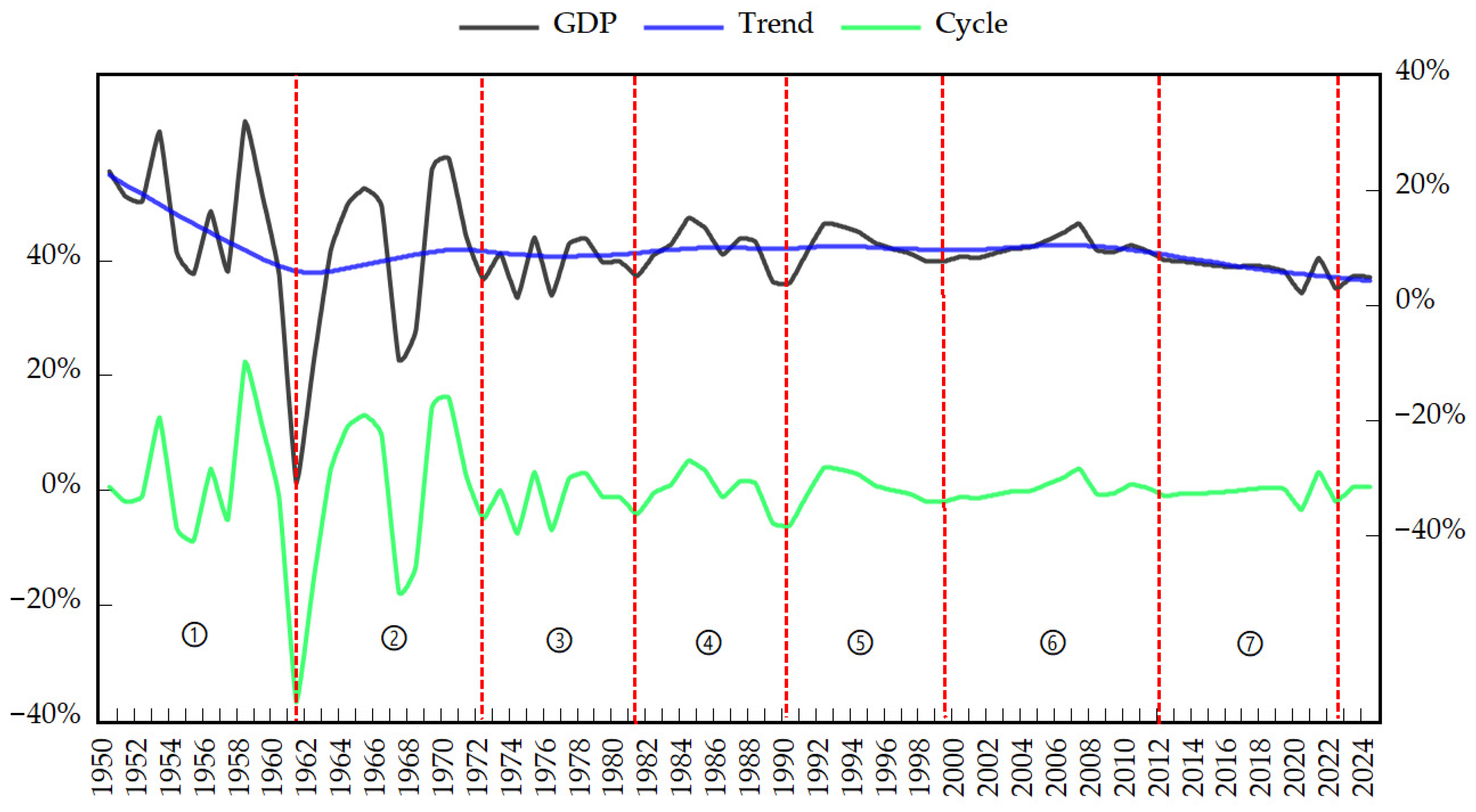
We apply the HP Filter to the GDP growth rate of China’s economy from 1950 to 2024, with the results shown in Figure 1. The horizontal axis denotes the time series, while the left vertical axis shows the GDP growth rate after HP filtering, and the right axis indicates the trend component and the actual GDP growth rate. The black dotted line plots actual GDP growth, the green dotted line represents the cyclical component, and the blue dotted line indicates the long-term trend. Figure 1 identifies seven distinct economic cycles in actual GDP growth: 1951–1961, 1961–1972, 1972–1981, 1981–1991, 1991–2000, 2000–2012, and 2012–2022, labeled as cycles ①, ②, ③, ④, ⑤, ⑥, and ⑦, respectively. The vertical red lines mark the initiation points of these cycles. It can be observed that economic cycles prior to 1972 exhibited pronounced boom-bust volatility, primarily driven by frequent political movements. The growth rate trend descended from its initial level, began recovering in 1961, and subsequently stabilized post-1972. China’s unique institutional characteristics—including government policy interventions, state-owned enterprise investment behaviors, and financial repression—significantly shape these economic fluctuations.

Figure 2 plots the cyclical components of China’s real GDP growth extracted using the HP filter, the Christiano–Fitzgerald (CF) filter, and the Baxter–King (BK) filter. The results demonstrate a striking concordance in the identification of China’s Juglar cycles. Specifically, the timing of the major peaks and troughs is remarkably consistent across all three methods. The visual alignment is corroborated by quantitative measures. The pairwise correlation coefficients between the cyclical series all exceed 0.85, indicating a very strong positive linear relationship. Therefore, we conclude that the chronology of Juglar cycles in China is robust and not sensitive to the choice of detrending algorithm. The evidence strongly suggests that these medium-term fluctuations are an inherent feature of the Chinese macroeconomic data rather than a statistical artifact.

Using Juglar’s methodology, we identify seven complete Juglar cycles in China’s economic trajectory from 1951 to 2024, as presented in

Table 2. Seven Juglar cycles from 1951 to 2024 in China.

Juglar Cycle (Years)	Duration (Years)	Kitchin Cycle (Years)	Duration (Years)
1951–1961	10	1951–1955	4
		1955–1957	2
		1957–1961	4
1961–1972	11	1961–1967	6
		1967–1972	5
1972–1981	9	1972–1976	4
		1976–1981	5
1981–1991	10	1981–1986	5
		1986–1991	5
1991–2000	9	1991–1995	4
		1995–2000	5
2000–2012	12	2000–2003	3
		2003–2006	3
		2006–2012	6
2012–2022	10	2012–2016	4
		2016–2020	4
		2020–2022	2
2022–	-	-	-

.

The first Juglar cycle (1951–1961) spanned 10 years and comprised three Kitchin cycles of 4, 2, and 4 years, respectively. During the recovery and boom phase (1951–1958), state-directed investment in heavy industry and infrastructure was channeled through the centralized planning system, supported by Soviet-aided projects and the First Five-Year Plan. This phase reached its zenith in 1958 with the launch of the Great Leap Forward. Subsequently, a severe Crisis phase (1959–1961) occurred, where the unsustainable policies led to a dramatic economic contraction.

The second Juglar cycle (1961–1972) lasted 11 years and encompassed two Kitchin cycles of 5 and 6 years. Its average annual GDP growth rate was 9.74%, peaking in 1970 at 25.7%. The cycle’s phases unfolded as follows: The recovery phase (1961–1964) featured a gradual rebound of public investment and economic activity following the previous crisis, as policy adjustments were implemented to stabilize the economy. The subsequent boom phase (1965–1966) experienced a significant acceleration in investment, particularly in defense and ‘Third Front’ construction, which drove economic expansion. A sharp crisis phase ensued (1967–1968), where political turmoil severely disrupted normal industrial production and investment activities, leading to a substantial economic contraction. The final recovery phase (1969–1972) was marked by a return to relative political stability and planned development. Investment and industrial output gradually recovered, culminating in a period of overheating around 1970 before growth moderated towards the end of the cycle.

The third Juglar cycle (1972–1981) spanned nine years, consisting of two Kitchin cycles of four and five years, respectively. Its average annual GDP growth rate was 7.46%. The recovery phase (1972–1976) featured moderate economic revitalization through strategic industrial investment, establishing a foundation for expansion with GDP growth averaging 4.0%. The boom phase (1977–1979) witnessed accelerated investment in comprehensive industrialization, pushing economic expansion to a peak growth of 13.19% in 1978. The crisis phase (1980–1981) emerged as structural imbalances required investment recalibration and policy adjustment, with growth moderating to an average of 8.2% during this consolidation period.

The fourth Juglar cycle (1981–1991) spanned ten years with 9.75% average annual GDP growth, encompassing two five-year Kitchin cycles. FAI grew at 18.2% annually with high volatility. The recovery phase (1982–1984) saw investment growth at 24.1% annually as reforms took hold. The boom phase (1985–1988) featured investment peaks above 27.6%, driving expansion but accumulating inflationary pressures. The crisis phase (1989–1991) experienced sharp investment contraction to 6.36% annual growth during economic adjustment. This cycle demonstrated high volatility with GDP growth ranging from 3.9% to 15.2%, reflecting investment-driven cyclical patterns throughout the reform period. This phase represented the initial stage of economic system reform, during which inflation and unemployment emerged as major challenges.

The fifth Juglar cycle (1991–2000) spanned 9 years with 10.58% average annual GDP growth, consisting of two Kitchin cycles of 4 and 5 years, respectively. FAI maintained strong growth at 23.9% annually with significantly lower volatility. During the recovery phase (1991–1992), investment growth rebounded to 34.4% annually as market reforms deepened. The boom phase (1993–1996) was characterized by sustained high investment growth at 31.1% annually, driving economic expansion while maintaining relative stability. The crisis phase (1997–2000) experienced moderated investment growth at 9.52% annually during the Asian Financial Crisis, demonstrating China’s enhanced macroeconomic resilience. This cycle exhibited moderated volatility with GDP growth ranging from 7.6% to 14.2%, reflecting China’s increasing maturity in managing investment-driven business cycles through market-oriented reforms.

The sixth Juglar cycle (2000–2012) spanned 12 years with 10.12% average annual GDP growth, encompassing three Kitchin cycles of 3, 3, and 6 years. FAI maintained robust growth at 19.8% annually, driven by infrastructure and real estate investment. The recovery phase (2000–2003) saw investment growth at 16% annually following WTO accession. The boom phase (2004–2007) featured investment peaks of 21.8% annually, fueling rapid economic expansion. The crisis phase (2008–2009) was triggered by the Global Financial Crisis, causing a sharp but brief economic contraction. In response, the Chinese government implemented a ¥4 trillion stimulus package in November 2008, with over 80% of which was directed toward infrastructure and real estate investment. This was followed by continuous policy refinements that formed a comprehensive crisis mitigation framework. This cycle exhibited sustained growth with GDP ranging from 7.9% to 14.2%, demonstrating the maturity of the investment-driven growth model during China’s accelerated globalization.

The seventh Juglar cycle (2012–2022) spanned 10 years with 6.72% average annual GDP growth, encompassing three Kitchin cycles of 3, 3, and 6 years. FAI growth moderated to 8.5% annually, reflecting the ongoing economic transition. The recovery phase (2012–2014) saw investment growth at 16% annually amid post-stimulus adjustment. The boom phase (2015–2018) featured stable investment growth at 6.9% annually, supporting quality-focused development. The crisis phase (2019–2022) experienced investment slowdown to 4.34% annually during trade tensions and the pandemic. This cycle showed moderated volatility with GDP growth ranging from 5.1% to 13.4%, reflecting China’s economic transition from high-speed to high-quality development.

The period from 2022 to 2024 exhibits characteristics that may indicate the early stages of a new Juglar cycle. However, definitive classification must await the availability of complete data and a clearer manifestation of cyclical phases.

4.3. The Role of Investment and Industrial Structure

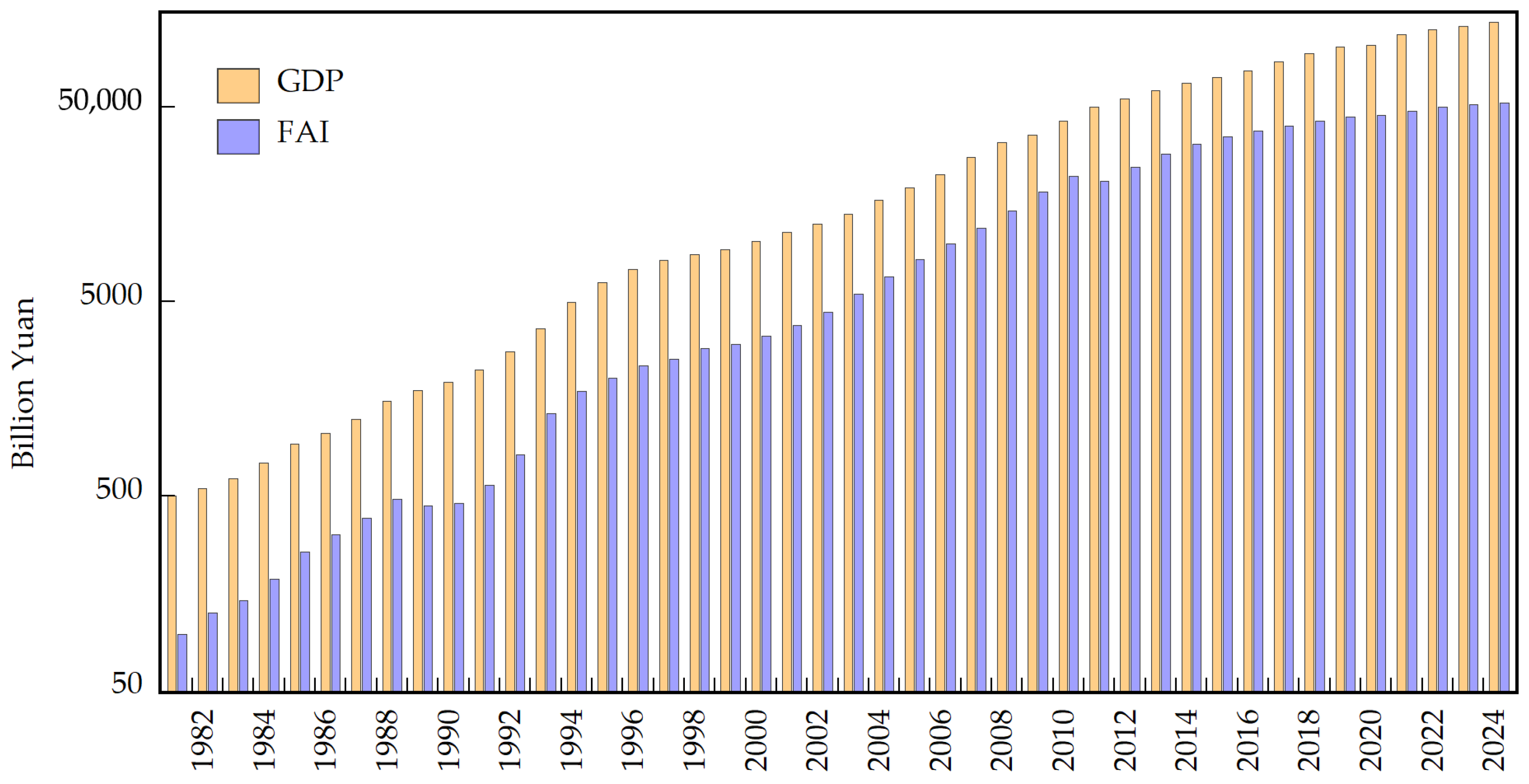
The time series data for GDP and FAI from 1981 to 2024 were analyzed. The data were sourced from various issues of the China Statistical Yearbook and the official website of the National Bureau of Statistics of China (https://www.stats.gov.cn/; accessed on 17 March 2025). As illustrated in Figure 3, GDP and FAI are represented by orange and blue bars, respectively. China’s FAI increased from 96.1 billion yuan in 1981 to 52.0916 trillion yuan in 2024, representing a 542-fold expansion. Over the same period, GDP grew from 494.5 billion yuan to 134.9085 trillion yuan, an increase of 273 times. Figure 3 demonstrates that both indicators exhibit nearly parallel growth trajectories. Following the implementation of the reform and opening-up policy in 1978, China experienced rapid economic development, with annual growth rates typically ranging between 8% and 10% [71]. By embracing market economy principles, the country significantly increased total social FAI, which played a critical role in driving economic growth. Figure 4 identifies four distinct Juglar cycles in total social FAI: 1981–1989, 1989–1999, 1999–2011, and 2011–2020, labeled as cycles ①, ②, ③, and ④, respectively. The vertical lines mark the initiation points of these cycles. Notably, these investment cycles precede corresponding fluctuations in the GDP growth rate by 1–2 years, indicating a delayed economic impact of capital formation.

Industrial structure refers to the composition and configuration of various material production sectors within the national economy, including their respective shares in total social production. China’s industrial structure specifically denotes the proportional relationships among agriculture, light industry, and heavy industry. The primary sector encompasses agriculture, forestry, animal husbandry, and fisheries. The secondary sector includes mining, manufacturing, electricity, gas, and water supply industries, as well as construction. The tertiary sector encompasses all other economic activities beyond the primary and secondary sectors, including the proportional relationships between distribution-related sectors and services supporting production and daily life.

Figure 5 displays the trend of GDP and the added values of the three industries from 1978 to 2024. The required data were collected from the issues of the China Statistical Yearbook and the official website of the National Bureau of Statistics of China (https://www.stats.gov.cn/ (accessed on 17 March 2025)). The black curve represents GDP, the red curve represents the added value of the primary industry (PIVA), the blue curve represents the added value of the secondary industry (SIVA), and the green curve represents the added value of the tertiary industry (TIVA). Figure 6 shows the proportion of added value of the three industries to GDP. The red, blue, and green curves represent the proportion of added value from the three major industries to GDP. These figures reveal that since the economic reforms began in 1978, China’s economy has embarked on a path of rapid development, with continuous growth in GDP and the added value of the primary, secondary, and tertiary industries. The industrial structure has undergone profound adjustments and optimizations, resulting in significant changes in the proportion of added value from these three sectors to GDP.

Since the reform and opening-up policy began in 1978, China’s economy has embarked on a high-speed development track, with GDP and the added value of the primary, secondary, and tertiary industries continuously increasing. The industrial structure has undergone deep adjustments and optimizations, leading to significant changes in the proportion of added value of the three industries to GDP. The proportion of the primary industry has been steadily declining; in 1978, it accounted for 27.69% of GDP, dropping to 14.68% by 2000. In the 21st century, this ratio continued to decline, reaching just 6.78% by the end of 2024. This trend reflects the gradual reduction in agriculture’s share in the national economy due to technological advances and industrialization progress. Despite this, agricultural modernization accelerated through measures like technological empowerment and large-scale operations, which led to continuous improvements in production efficiency and quality. The secondary industry displayed phase-specific fluctuations from 1978 to 2006; the proportion of added value of the secondary industry in GDP showed an upward trend, peaking at 47.56% in 2006. The subsequent decline was largely driven by strategic national policies, specifically the Supply-Side Structural Reforms and stringent environmental protection laws enacted after 2015. These policies deliberately phased out excess capacity in heavy industries (e.g., steel, coal) and reoriented investment towards advanced manufacturing and services, accelerating the sector’s relative contraction.

Subsequently, its proportion gradually decreased to 36.48% by 2024 due to economic restructuring and environmental policies. During this period, China’s industry transitioned from traditional extensive models to modern intensive ones, and from labor-intensive to technology and capital-intensive structures. On one hand, traditional industries have upgraded through technological transformation, phasing out outdated capacities, and enhancing production efficiency and product quality.

On the other hand, emerging industries such as high-end equipment manufacturing, new energy, and new materials have expanded rapidly, becoming new growth points in the industrial economy. The tertiary sector has also undergone significant expansion, increasing its share of GDP from 24.6% in 1978 to 39.79% by 2000. By 2024, it accounted for a dominant 56.75% share, underscoring its pivotal role in the economic structure. Continuously propelled by technological innovation and consumption upgrades, high-tech and modern services within this sector are expected to serve as key engines for promoting high-quality economic development in China. The economic composition in 2024 (primary: 6.78%, secondary: 36.48%, tertiary: 56.75%) reflects this shift towards a new development paradigm. This structure aligns with China’s broader strategic goals of high-quality growth, underpinned by the dual-circulation strategy that leverages a robust domestic service sector, and supports the transition to a greener economy in line with carbon neutrality objectives.

As illustrated in the annotated Figure 6, these structural shifts are closely linked to key historical policy milestones. The accelerated decline of the primary sector and the rapid expansion of the secondary industry after 2001, for instance, can be largely attributed to China’s accession to the WTO, which more deeply integrated the nation into global supply chains. Similarly, the stimulus measures implemented after the 2008 Global Financial Crisis temporarily boosted secondary-industry investment. The more recent decline in the secondary sector’s proportion and the simultaneous rise of the tertiary sector, evident from around 2010 onward, are consistent with strategic policy shifts towards environmental protection and a rebalancing of the economy toward consumption and services.

Furthermore, from a macroeconomic perspective, a given total resource endowment will yield differing economic benefits depending on allocation methods and structural arrangements. In other words, under identical social resource endowments, different industrial structures lead to distinct economic growth outcomes, with the structure of industrial investment representing a critical determinant of economic growth.

5. Empirical Analysis

In this study, we adopted a VECM framework to examine the dynamic interrelationships among GDP, FAI, GFE, TFP, and ISU in China, covering the period from 1981 to 2024. All econometric analyses were conducted using EViews 13. The VAR model is suitable for capturing short-term interactions among stationary variables without imposing a priori structural restrictions. However, when variables are non-stationary but cointegrated, a VECM is preferred, since it incorporates both the short-term dynamics and the long-term equilibrium relationships among the variables.

5.1. Unit Root Tests and Data Transformation

To mitigate potential heteroscedasticity and facilitate the interpretation of elasticity coefficients, the non-stationary time series for GDP, FAI, and GFE are transformed into natural logarithmic form, denoted as LNGDP, LNFAI, and LNGFE, respectively. Because regression analysis involving non-stationary variables may yield spurious results, testing for stationarity is an essential preliminary step in empirical modeling. We apply the Augmented Dickey–Fuller (ADF) test to examine the presence of unit roots in each variable. The test specifications include an intercept and a linear trend for variables in levels, and only an intercept for the first-differenced variables, with critical values derived from MacKinnon [72]. As summarized in

Table 3. Unit Root Test Results.

Variable Sequence	ADF-Statistics	Critical Value (5%)	Prob. *	Phillips-Perron Statistics	Critical Value (5%)	Prob. *	Conclusion
LNGDP	−0.9790	−3.5207	0.9362	0.1239	−3.5180	0.9966	Nonstationary
DLNGDP	−3.6091	−2.9331	0.0410	−3.6092	−2.9331	0.0331	Stationary
LNFAI	−0.8569	−3.5207	0.9515	−0.3389	−3.5181	0.9868	Nonstationary
DLNFAI	−3.8913	−2.9331	0.0212	−3.3139	−2.9331	0.0205	Stationary
LNGFE	−0.0414	−3.5207	0.9943	−0.0198	−3.5181	0.9947	Nonstationary
DLNGFE	−3.5847	−2.9331	0.0393	−3.0033	−2.9331	0.0427	Stationary
TFP	−1.7461	−3.5207	0.7130	−1.9987	−3.5181	0.5854	Nonstationary
DTFP	−4.9008	−2.9331	0.0015	−4.9174	−2.9331	0.0002	Stationary
ISU	−1.8542	−3.5207	0.6601	−1.4649	−3.5181	0.8263	Nonstationary
DISU	−4.5316	−2.9331	0.0041	−4.4937	−2.9331	0.0008	Stationary

Note: the prob. marked with * are MacKinnon’s one-sided p-values [72].

, the ADF test results indicate that the null hypothesis of a unit root cannot be rejected for all level series—LNGDP, LNFAI, LNGFE, TFP, and ISU—as their test statistics exceed the 5% critical values. By contrast, the first-differenced series reject the null hypothesis at the 5% significance level, since their ADF statistics fall below the corresponding critical values. This confirms that all first-differenced series are stationary, and thus the original variables are integrated of order one, I(1). To ensure the robustness of these findings, we also conduct Phillips–Perron (PP) tests, which employ a non-parametric correction to account for potential heteroskedasticity and serial correlation. The results from the PP tests, also presented in Table 3, are fully consistent with those of the ADF tests, providing strong support for the conclusion that all variables are I(1).

5.2. Determination of Optimal Lag Length

Prior to conducting cointegration analysis, the appropriate lag length (p) for the underlying vector autoregression (VAR) model must be determined. This is a critical step, since an underspecified lag structure may fail to capture the data-generating process and render the residuals serially correlated, while an overspecified model can lead to inefficiency and a loss of degrees of freedom. To identify the optimal lag order, we estimate an unrestricted VAR model in levels that includes the five core variables (LNGDP, LNFAI, LNGFE, TFP, ISU) and the set of break dummy variables (Dum1992, Dum1997, Dum2001, Dum2008) as exogenous regressors. This study employs a lag length ranging from 0 to 3. The selection is based on a suite of information criteria such as Likelihood Ratio (LR), Final Prediction Error (FPE), Akaike Information Criterion (AIC), Schwarz Information Criterion (SC), and Hannan-Quinn Criterion (HQ), with the results summarized in

Table 4. Optimal Lag Test.

Lag	LogL	LR	FPE	AIC	SC	HQ
0	68.11948	NA	3.17 × 10−8	−3.078999	2.870027	−3.002903
1	384.9925	541.0028	2.10 × 10−14	−17.31671	−16.06288 *	−16.86013
2	422.6687	55.13582 *	1.20 × 10−14 *	−17.93506	−15.63636	−17.09800 *
3	447.7308	30.56362	1.39 × 10−14	−17.93809 *	−14.59453	−16.72055

Note: the asterisk (*) indicates the selected lag.

. As shown in Table 4, the optimal lag length test indicates that a lag of 2 is selected by most information criteria (LR, FPE, AIC, and HQ). Therefore, the model used in this study is the VECM with a lag length of 2. The error correction term will thus have a lag of 1, denoted as VECM(1).

5.3. Cointegration Test with Structural Breaks

The finding that all variables are I(1) validates the pursuit of a long-run equilibrium relationship. However, standard cointegration tests like the Johansen procedure are prone to pre-test bias if structural breaks are present but ignored. China’s economic landscape over the 1981–2024 period has been shaped by pivotal events, such as the 1992 Southern Tour, the 1997 Asian Financial Crisis, the 2001 WTO accession, and the 2008 Global Financial Crisis—which represent exogenous shocks and major policy shifts with the potential to induce permanent structural changes in the long-run equilibrium [73]. To account for these known structural breaks, we incorporate step dummy variables to capture permanent shifts in the long-run equilibrium relationship following these events: (1) Dum1992: 1 from 1992 onwards, 0 otherwise (Southern Tour Speech); (2) Dum1997: 1 from 1997 onwards, 0 otherwise (Asian Financial Crisis); (3) Dum2001: 1 from 2001 onwards, 0 otherwise (WTO accession); (4) Dum2008: 1 from 2008 onwards, 0 otherwise (Global Financial Crisis). These dummy variables are included in the cointegration space as exogenous components.

The results of the Johansen test with these break dummies are presented in

Table 5. Cointegration Rank Test.

Hypothesized No. of CE(s)	Eigenvalue	Trace Statistic	Critical Value (5%)	Prob. Critical Value	Max-Eigen Statistic	Critical Value (5%)	Prob. Critical Value
None *	0.566635	85.71111	69.81889	0.0016	35.11935	33.87687	0.0354
At most 1 *	0.373081	50.59177	47.85613	0.0270	19.61140	27.58434	0.3686
At most 2 *	0.349219	30.98037	29.79707	0.0364	18.04242	21.13162	0.1283
At most 3	0.171723	12.93794	15.49471	0.1171	7.913122	14.26460	0.3876
At most 4 *	0.112759	5.024822	3.841465	0.0250	5.024822	3.841465	0.0250

Note: the asterisk (*) indicates rejection of the null hypothesis at the 5% significance level.

. As shown in the table, the trace statistic rejects the null hypothesis of no cointegration at the 5% significance level for the assumptions of r = 0, r ≤ 1, and r ≤ 2, as the test values exceed their critical values with associated probabilities below 5%. This suggests the presence of three cointegrating equations. In contrast, the maximum eigenvalue test rejects the null hypothesis of no cointegration only for the r = 0 hypothesis, indicating exactly one cointegrating equation at the 5% significance level. Faced with these mixed results, we proceed based on the maximum eigenvalue test result and the principle of parsimony, concluding there is one cointegrating relation at the 5% significance level. This confirms a stable long-run relationship among the variables even when accounting for structural breaks, justifying the subsequent use of the VECM for further analysis.

Given the evidence of a single cointegrating relationship, we proceed to estimate the corresponding long-run equilibrium. The normalized cointegrating equation is as follows (standard errors in parentheses):

$$\begin{array}{c}LNGDP=0.887094LNFAI-0.084177LNGFE-0.255779TFP+0.844781ISU\\ \left(0.07702\right)\hspace{1em}\hspace{1em} \left(0.10320\right)\hspace{1em}\hspace{1em} \left(0.38819\right)\hspace{1em}\hspace{1em} \left(0.12423\right)\end{array}$$

(12)

The normalized cointegrating coefficients elucidate the long-run elasticities, revealing the sustained responsiveness of economic output to its fundamental drivers. The analysis demonstrates that FAI exerts the strongest marginal influence on long-term growth, with a 1% increase in FAI associated with a 0.88% rise in GDP, ceteris paribus. This dominant elasticity reflects China’s investment-intensive growth paradigm, underscoring the pivotal role of capital accumulation in driving economic expansion. Furthermore, a one-unit advancement in the ISU index—signifying a reallocation of resources towards more advanced, high-value-added sectors—is linked to a 0.84% expansion in output. This statistically significant relationship confirms that strategic structural transformation serves as a genuine driver of growth, enhancing overall allocative efficiency and building a more resilient economic foundation.

The positive and statistically significant coefficients on LNFAI, TFP, and ISU indicate that FAI, technological progress, and ISU are pivotal drivers of long-term economic growth in China. Among these, FAI exhibits the largest long-run marginal effect on output, highlighting its fundamental role in China’s growth model over the study period. The result for ISU is particularly informative, indicating that the strategic shift of resources from traditional, low-value-added sectors towards more advanced, high-productivity industries has been a critical component of China’s development model. This structural transformation enhances allocative efficiency and strengthens linkages with technological innovation, as captured by TFP.

However, the negative and statistically significant coefficient on LNGFE presents a more nuanced finding, highlighting a potential tension within the growth model. A plausible explanation is the crowding-out effect, whereby increased government borrowing drives up interest rates and deters more efficient private investment, which is essential for sustaining the industrial upgrading process. Alternatively, this result could point to inefficiencies in public spending, if funds are misallocated to sustain unproductive state-owned enterprises in obsolete sectors rather than being channeled into productivity-enhancing sectors that support structural upgrading. This finding underscores the complex trade-off between the scale of government expenditure and its qualitative impact on economic growth, suggesting that the composition of public spending may be just as important as its volume for fostering sustainable development.

5.4. Short-Run Dynamics and Adjustment to Equilibrium

The short-run dynamics of economic growth, derived from the VECM, are presented in

Table 6. Short-Run Estimation Results of the VECM (Dependent Variable: D(LNGDP)).

Variable	Coefficient	Std. Error	T-Statistic
ECT(-1)	−0.167499	0.08714	−1.92226
DLNGDP(-1)	−0.116028	0.25433	−0.45620
DLNFAI(-1)	0.173048	0.07901	2.19031
DTFP(-1)	0.522799	0.23701	2.20583
DISU(-1)	−0.228693	0.17418	−1.31300
DLNGFE(-1)	0.298166	0.19140	1.55779
C	0.126746	0.03013	4.20691
DUM1992	0.015589	0.02239	0.69629
DUM1997	−0.073139	0.03902	−1.87442
DUM2001	−0.001947	0.02932	−0.06641
DUM2008	−0.012753	0.02001	−0.63729
R-squared	0.745157
Adjusted R-squared	0.662950
F.statistic	9.064376
Log likelihood	85.19059

. The core of the VECM is the Error Correction Term (ECT(-1)), which is constructed from the long-run cointegrating relationship (Equation (12)) and captures the previous period’s deviation from equilibrium. The negative and statistically significant coefficient on ECT(-1) is a central finding of our model. With a value of −0.167 and significant at the 10% level (t-statistic = −1.92), it fulfills the critical condition for a valid error correction mechanism, thereby confirming the existence of a stable long-run relationship among the variables. This coefficient has a clear economic interpretation: approximately 16.7% of any disequilibrium in one period is corrected in the next. The moderate magnitude of this adjustment speed suggests that the Chinese economy exhibits inherent rigidities—potentially reflecting policy implementation lags or the long gestation period of investments—that slow the return to equilibrium following a shock.

Among the short-run drivers, both fixed asset investment (DLNFAI(-1)) and total factor productivity (DTFP(-1)) exhibit positive and statistically significant effects on GDP growth at the 5% level, with coefficients of 0.173 and 0.523, respectively. These results indicate that investment and productivity improvements serve as important short-run catalysts for economic expansion. Government fiscal expenditure (DLNGFE(-1)) also shows a positive albeit marginally insignificant effect (coefficient = 0.298, t-statistic = 1.56). The model demonstrates a reasonably good overall fit, with an adjusted R-squared of 0.663, meaning that the specified variables explain approximately two-thirds of the short-term variation in GDP growth. The overall significance of the model is confirmed by the F-statistic of 9.064, which is significant at conventional levels. None of the included dummy variables for structural breaks reach statistical significance in the short-run equation, implying that these events did not exert immediate impacts on GDP growth beyond what is captured through the model’s other explanatory variables.

5.5. Model Diagnostics and Analysis of Dynamic Relationships

Following the estimation of the VECM, this section presents a comprehensive analysis of the dynamic interrelationships among the variables. We first subject the model to a battery of diagnostic tests to ensure its statistical adequacy and stability. Subsequently, we employ statistical Granger causality tests, impulse response functions (IRFs), and forecast error variance decomposition (FEVD) to unravel the short-term causal linkages and dynamic responses within the system.

5.5.1. Stability and Residual Diagnostics

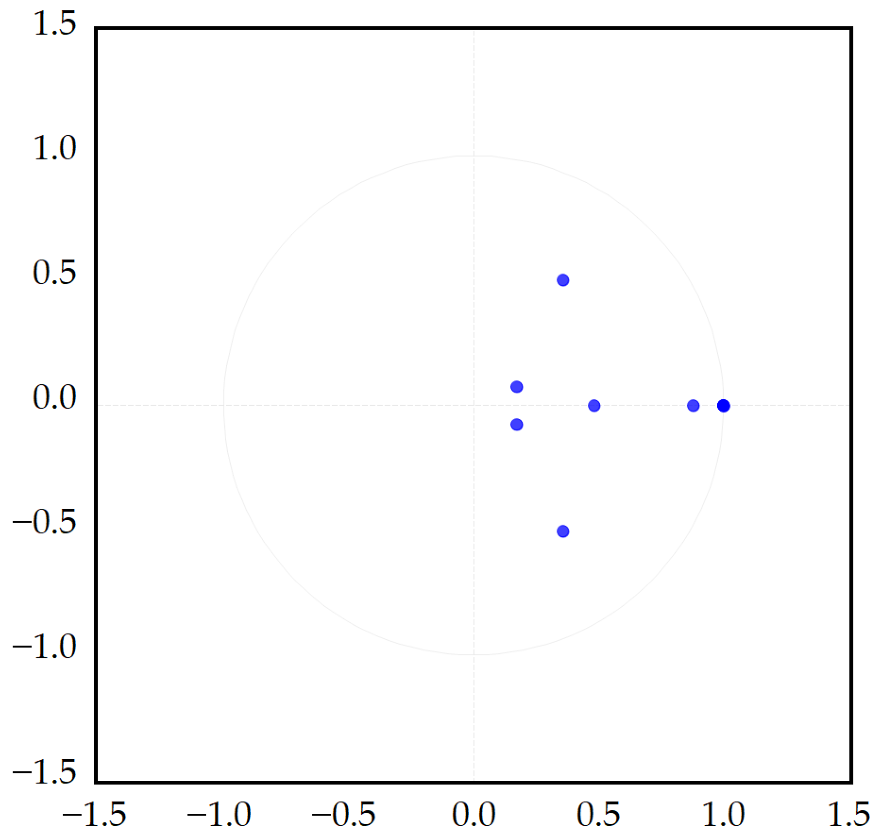
To ensure the reliability of the VECM estimates, we examine the stability condition of the model. Figure 7 displays the inverse roots of the characteristic AR polynomial. Consistent with theoretical expectations for a cointegrated system with five I(1) variables and one cointegrating relation, exactly four roots are found to lie on the unit circle. All remaining roots have moduli strictly less than unity and are located well inside the unit circle. This confirms that our VECM specification is stable and that the impulse response functions will converge, thereby ensuring valid economic inference.

In addition, a series of diagnostic tests were conducted on the residuals to ensure the robustness and statistical adequacy of the estimated model. The results, summarized in

Table 7. VECM Residual Diagnostic Tests.

Test	Test Statistic	p-Value	Conclusion
Portmanteau LM Test (autocorrelation)	Rao F-stat (25, 83.2) = 0.607572	0.9205	No serial correlation
White’s Test (heteroskedasticity)	X2 (240) = 231.48	0.6417	No heteroskedasticity

, confirm that the model is well-specified and satisfies the key assumptions of classical linear regression. The Portmanteau test for serial correlation, based on the Rao F-statistic, fails to reject the null hypothesis of no autocorrelation up to the chosen lag order (F (25, 83.2) = 0.608, p = 0.921). White’s test for heteroskedasticity fails to reject the null hypothesis of homoskedasticity (χ² (240) = 231.48, p = 0.642). The absence of evidence for heteroskedasticity, based on these diagnostic tests, suggests that the model’s residuals are well-behaved for the purpose of our analysis. The absence of serial correlation and heteroskedasticity ensures that the parameter estimates are efficient and the standard errors are reliable. Consequently, the model passes all critical diagnostic checks, providing strong support for the subsequent analysis of impulse responses and variance decomposition.

5.5.2. Granger Causality Analysis

To investigate the short-term causal dynamics between the variables, we conduct statistical Granger causality tests within the VECM framework. These Wald tests evaluate whether the lagged values of one variable can help to predict another variable in the system, holding other factors constant. The results, summarized in

Table 8. Granger Causality.

Dependent Variable	Excluded	Chi-sq (χ2)	df	Prob.
D(LNGDP)	D(LNFAI)	4.797444	1	0.0285
	D(LNGFE)	2.426695	1	0.1193
	D(TFP)	4.865667	1	0.0274
	D(ISU)	1.723973	1	0.1892
	All	16.03219	4	0.0030
D(LNFAI)	D(LNGDP)	0.410955	1	0.5215
	D(LNGFE)	0.099857	1	0.7520
	D(TFP)	0.133792	1	0.7145
	D(ISU)	0.425194	1	0.5144
	All	1.746133	4	0.7823
D(LNGFE)	D(LNGDP)	0.012492	1	0.9110
	D(LNFAI)	2.247792	1	0.1338
	D(TFP)	4.020766	1	0.0449
	D(ISU)	0.216262	1	0.6419
	All	8.892865	4	0.0638
D(TFP)	D(LNGDP)	0.863628	1	0.3527
	D(LNFAI)	3.566215	1	0.0590
	D(LNGFE)	0.005558	1	0.9406
	D(ISU)	0.004226	1	0.9482
	All	4.114832	4	0.3907
D(ISU)	D(LNGDP)	0.094195	1	0.7589
	D(LNFAI)	0.249458	1	0.6175
	D(LNGFE)	0.134505	1	0.7138
	D(TFP)	4.969123	1	0.0258
	All	5.078873	4	0.2793

, reveal a unidirectional predictive structure centered on FAI in the short term. The most robust finding is that FAI exerts a significant short-run driving effect on the economy. It is a strong short-run Granger cause of LNGDP at the 5% significance level (χ² = 4.7974, p = 0.0285). Conversely, and of equal importance, there is no evidence of reverse causality. The hypothesis that “D(LNGDP) does not Granger cause D(LNFAI)” cannot be rejected (p-value = 0.5215). This establishes a unidirectional causal relationship running from investment to GDP, but not from GDP back to investment in the short run. This asymmetry is consistent with the view of investment as a leading indicator within this framework. Furthermore, LNFAI is also a significant Granger cause of TFP at the 10% level (p = 0.059). This indicates that shocks to investment have broad-based effects, influencing not only output but also technological efficiency in the short term. By contrast, GDP itself does not Granger-cause any of the other variables in the short run, as all corresponding p-values are statistically insignificant (p > 0.10). This reinforces the leading role of investment in this short-run predictive system. The joint test for the GDP equation is highly significant (χ² = 16.03, p = 0.030), confirming that the included variables collectively have significant predictive power for short-run economic growth. In addition, TFP growth also significantly predicts changes in the GFE and ISU, positioning it as a central node for broader economic dynamics beyond just growth. It should be emphasized that Granger causality indicates a predictive relationship rather than a proven cause-effect link.

In summary, the short-run dynamics are predominantly characterized by a unidirectional predictive relationship flowing from FAI to economic growth and productivity. This suggests that investment possesses a leading indicator property and underscores its potential role as a key short-term driver for the economy within our modeling framework, though the inherent endogeneity of investment cautions against strong causal claims.

The unidirectional causality from FAI to GDP is consistent with China’s policy-led growth model. This is because a significant portion of investment is directed by state policy for strategic development, causing investment to lead economic cycles rather than respond to them. Furthermore, the long gestation period of large-scale investments means that current FAI is determined by prior decisions and expectations, thereby weakening its short-term statistical feedback from concurrent GDP growth.

5.5.3. Impulse Response Analysis

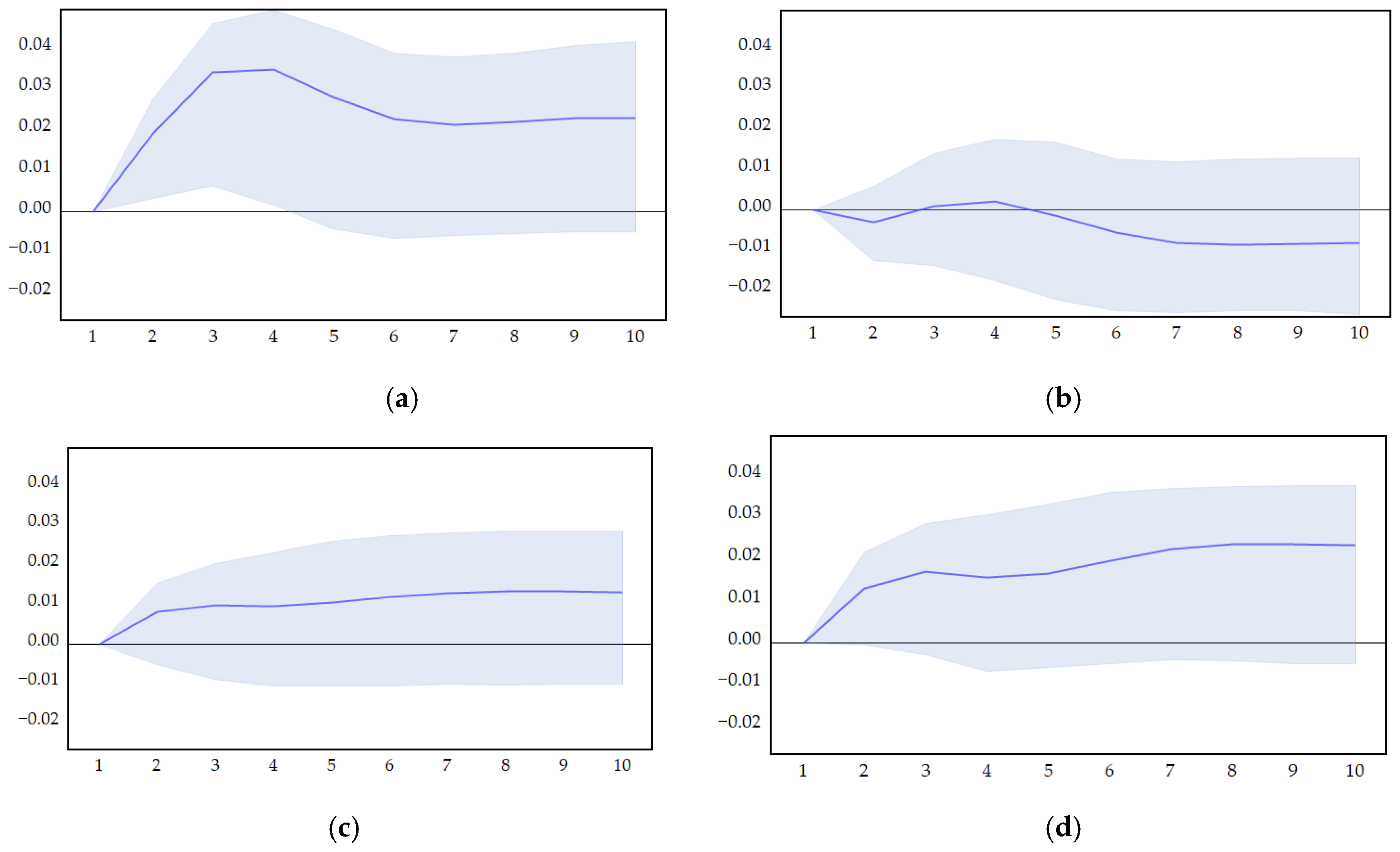
To trace the dynamic time path of the variables in response to economic shocks, we employ generalized impulse response functions (IRFs). Figure 8 depicts the response of GDP to a one standard deviation shock in the other variables. The solid blue line represents the point estimate of the response, while the shaded area denotes the 5% significance confidence band. The impact of FAI is positive from the initial periods (1–3), strengthening gradually before stabilizing around period 6 (see Figure 8a). This pattern reflects both the immediate demand-side stimulus and the sustained cumulative effect of investment, consistent with the theoretical investment multiplier mechanism whereby capital formation stimulates activity across industrial supply chains. In contrast, the response to industrial structure adjustment is initially negative (see Figure 8b), aligning with Schumpeter’s “creative destruction” framework. This short-term contraction represents the necessary transition cost as resources shift from less to more efficient sectors, with the destructive phase preceding the benefits of creative reorganization. The response to a government spending shock is positive but gradual (see Figure 8c), indicating the presence of implementation lags in fiscal policy and the slow propagation of the multiplier effect through successive rounds of consumption. Figure 8d indicates a positive and statistically significant effect of a TFP shock on GDP. Although the initial impact, though very small, is positive, the response increases substantially and monotonically over the subsequent periods before stabilizing around period 8. This finding is consistent with economic theory, which posits that innovations in productivity are a key driver of long-run economic output. The increasing trajectory suggests that the full positive effect of a TFP shock on GDP accumulates over time rather than occurring instantaneously. Taken together, the impulse response analysis corroborates that FAI is a pivotal driver of economic activity in China, generating strong positive output effects.

5.5.4. Variance Decomposition Analysis

Table 9. Variance Decomposition Test of GDP.

Variance Period	S.E.	GDP	FAI	GFE	TFP	ISU
1	0.037052	100.0000	0.000000	0.000000	0.000000	0.000000
2	0.068849	87.15437	6.889501	0.183310	4.827634	0.945189
3	0.098531	77.90688	13.27255	1.163587	6.903727	0.753263
4	0.122047	75.20936	15.45698	1.560980	7.144834	0.627838
5	0.140439	75.37821	15.19892	1.365284	7.348238	0.709355
6	0.156357	75.78228	14.24152	1.107580	7.871100	0.997523
7	0.171148	75.75298	13.37607	0.926719	8.587764	1.356468
8	0.185059	75.49518	12.79178	0.794445	9.263794	1.654800
9	0.198066	75.24196	12.41118	0.693757	9.785326	1.867778
10	0.210223	75.06666	12.12366	0.615901	10.16900	2.024781

presents the variance decomposition of GDP, showing the relative contributions of FAI, GFE, TFP, ISU, and GDP’s own innovations over several periods. In the first period, 100% of the variation in GDP is attributable to its own shocks. From period 2, however, other variables—FAI, GFE, TFP, and ISU—begin to account for a share of the fluctuation, though GDP itself remains the dominant source (87.15%). Over time, the influence of these external factors gradually increases. By period 4, FAI contributes 15.45%, making it the most significant external driver, while GFE, TFP, and ISU account for 1.56%, 7.14%, and 0.62%, respectively. By the 10th period, GDP’s own shocks explain 75.06% of the variation, with FAI, GFE, TFP, and ISU contributing 12.12%, 0.61%, 10.17%, and 2.02%, respectively.

The decomposition results reveal several important patterns. Among all variables, FAI remains the largest contributor to the forecast error variance of GDP. TFP is the third major contributor, exhibiting a clear and monotonically increasing influence over the forecast horizon. Its contribution grows from 4.83% in period 2 to 10.17% by the final period. This rising importance indicates that productivity gains, while less impactful than investment in the immediate short run, become an increasingly vital source of sustainable growth and cycle dynamics in the medium to long term. Additionally, ISU’s contribution indicates a steady upward trend, rising from initially negligible levels to 2.02% by period 10. This suggests that ISU acts as a long-term driver of GDP fluctuations, with its impact strengthening over time. Although its short-term effects are limited, ISU emerges as an important factor in the long run, following FAI and TFP.

6. Conclusions

This study has systematically identified and analyzed the operation of Juglar cycles in China through an integrated framework that incorporates investment, policy, productivity, and structural dimensions. Our empirical investigation yields several key conclusions that collectively address the research gap identified in the introduction regarding the need for a comprehensive, multi-faceted analysis of China’s medium-term fluctuations.

First, we confirm the enduring relevance of the Juglar cycle in explaining China’s medium-term fluctuations, in line with its investment-led growth model. The cyclical patterns, dating back to the 1950s and evolving through distinct phases up to 2024, are robust across alternative detrending methods and reflect the rhythmic pulsations of fixed asset investment. Notably, within China’s institutional context, these investment waves are predominantly state-initiated and policy-anchored, illustrating a transmission mechanism that is reconfigured relative to classic market-driven Juglar cycles.

Second, the long-run cointegration analysis reveals that FAI is the most powerful driver of economic output, underscoring the continued centrality of capital accumulation in China’s growth architecture. At the same time, industrial structure upgrading exerts a significant positive effect, confirming that structural transformation toward advanced sectors enhances allocative efficiency and output. In contrast, the negative long-run coefficient on government fiscal expenditure suggests subtle inefficiencies—likely arising from crowding-out effects or the misallocation of public resources—which can attenuate growth despite short-term stimulus intentions.

Third, the short-run dynamics and Granger causality tests reveal a unidirectional predictive relationship from investment to GDP, implying that shocks to FAI—which often stem from policy changes—play a leading role in initiating economic fluctuations. The error correction mechanism is statistically significant but of moderate magnitude, indicating a sluggish adjustment to equilibrium and inherent rigidities within the economic system.

Finally, variance decomposition and impulse response analyses map out the temporal dynamics of these relationships: while FAI dominates in explaining output variation in the earlier horizons, the contribution of TFP grows steadily over time, reflecting a gradual shift toward a productivity-intensive growth model.

These findings carry salient policy implications. The government’s recent initiative to promote large-scale equipment upgrades resonates directly with the Juglar cycle’s theoretical core and is likely to instigate a new upswing. However, policymakers should recognize the diminishing returns and potential distortions from prolonged investment-led stimulus. Enhancing the quality—not merely the volume—of public expenditure, accelerating structural reforms, and fostering innovation-led productivity are essential to mitigate cyclical downturns and ensure sustainable growth.

The VECM framework, while accounting for structural breaks, does not fully resolve endogeneity, structural identification, and nonlinearities or regime shifts, which is especially critical in a rapidly transforming economy like China. Moreover, the model omits external factors such as global demand shocks, financial spillovers, and foreign direct investment, which may also shape China’s business cycles and investment behavior.

This study acknowledges limitations including the use of macro-aggregate data, which may mask regional and sectoral heterogeneities. Future research could incorporate disaggregated investment data, integrate financial variables, or develop regional-level models to better capture spatial dimensions of fluctuations. Employing nonlinear or time-varying parameter models, along with international variables, would be particularly valuable for understanding how major future trends—such as technological dependence and the green transformation—are likely to reshape industrial structure and investment cycle dynamics, thereby providing a more comprehensive understanding of medium-term cycles in open and heterogeneous economies.

Nevertheless, this analysis offers a robust empirical foundation for examining China’s distinctive economic rhythms and highlights the importance of blending classical theory with institutional specificity to decipher the cycles of one of the world’s most influential economies. Understanding these rhythms is therefore essential not only for navigating China’s future economic development but also for anticipating its profound implications for the global economy.

References

1. Kirby, W.C. Continuity and change in modern China: Economic planning on the Mainland and on Taiwan, 1943–1958. Aust. J. Chin. Aff. 1990, 24, 121–141. [Google Scholar] [CrossRef]
2. Wei, C.G. The economic cooperation administration, the state department, and the American presence in China, 1948–1949. Pac. Hist. Rev. 2001, 70, 21–53. [Google Scholar] [CrossRef]
3. Davies, R.W.; Wheatcroft, S.G. Further thoughts on the first Soviet Five-Year Plan. Slavic Rev. 1975, 34, 790–802. [Google Scholar] [CrossRef]
4. Stone, D.R. The first five-year plan and the geography of soviet Defence industry. Eur. Asia Stud. 2005, 57, 1047–1063. [Google Scholar] [CrossRef]
5. Peterson, G. The Overseas Chinese Areas of Rural Guangdong and Socialist Transformation 1949–1956. Ph.D. Thesis, University of British Columbia, Vancouver, BC, Canada, 1986. [Google Scholar] [CrossRef]
6. Jianhui, L.; Hongxu, W. The origins of the general line for the transition period and of the acceleration of the Chinese socialist transformation in summer 1955. China Q. 2006, 187, 724–731. [Google Scholar] [CrossRef]
7. Zhang, T. A review on western studies on the socialist transformation in China. Chin. Stud. 2022, 11, 147–155. [Google Scholar] [CrossRef]
8. Li, W.; Yang, D.T. The great leap forward: Anatomy of a central planning disaster. J. Polit. Econ. 2005, 113, 840–877. [Google Scholar] [CrossRef]
9. Harrell, S. The four horsemen of the ecopocalypse: The agricultural ecology of the Great Leap Forward. Hum. Ecol. 2021, 49, 7–18. [Google Scholar] [CrossRef]
10. Bai, L.; Wu, L. Political conflict and development dynamics: Economic legacies of the cultural revolution. J. Econ. Hist. 2023, 83, 981–1017. [Google Scholar] [CrossRef]
11. Saich, T. China Under Reform, 1978–2000. In Governance and Politics of China, 1st ed.; Palgrave: London, UK, 2001; pp. 52–79. [Google Scholar] [CrossRef]
12. Lin, J.Y. The household responsibility system reform in China: A peasant’s institutional choice. Am. J. Agr. Econ. 1987, 69, 410–415. [Google Scholar] [CrossRef]
13. Lin, J.Y. The household responsibility system in China’s agricultural reform: A theoretical and empirical study. Econ. Dev. Cult. Change 1988, 36, S199–S224. [Google Scholar] [CrossRef]
14. Zengxian, W. How successful has state-owned enterprise reform been in China? Eur. Asia Stud. 1997, 49, 1237–1262. [Google Scholar] [CrossRef]
15. Brødsgaard, K.E.; Li, X. SOE reform in China: Past, present and future. Cph. J. Asian Stud. 2013, 31, 54–78. [Google Scholar] [CrossRef]
16. Lardy, N.R. The role of foreign trade and investment in China’s economic transformation. China Q. 1995, 144, 1065–1082. [Google Scholar] [CrossRef]
17. Khor, H.E. China—Macroeconomic cycles in the 1980S. China Econ. Rev. 1992, 3, 173–194. [Google Scholar] [CrossRef]
18. Komiya, R. Macroeconomic development of China: “Overheating” in 1984–1987 and problems for reform. J. Jpn. Int. Econ. 1989, 3, 64–121. [Google Scholar] [CrossRef]
19. Yu, Q. Economic fluctuation, macro control, and monetary policy in the transitional Chinese economy. J. Comp. Econ. 1997, 25, 180–195. [Google Scholar] [CrossRef]
20. Lu, Y.; Zhang, Y.; Cao, X.; Wang, C.; Wang, Y.; Zhang, M.; Zhang, Z. Forty years of reform and opening up: China’s progress toward a sustainable path. Sci. Adv. 2019, 5, eaau9413. [Google Scholar] [CrossRef]
21. Shi, Y.; Guo, S.; Sun, P. The role of infrastructure in China’s regional economic growth. J. Asian Econ. 2017, 49, 26–41. [Google Scholar] [CrossRef]
22. Bello, W. The Asian financial crisis: Causes, dynamics, prospects. J. Asia Pac. Econ. 1999, 4, 33–55. [Google Scholar] [CrossRef]
23. Yang, Y.; Tyers, R. The Asian crisis and economic change in China. Jpn. Econ Rev. 2001, 52, 491–510. [Google Scholar] [CrossRef]
24. Li, L.; Willett, T.D.; Zhang, N. The effects of the global financial crisis on China’ s financial market and macroeconomy. Econ. Res. Int. 2012, 2012, 961694. [Google Scholar] [CrossRef]
25. Zhang, J.; Chen, J. Introduction to China’s new normal economy. J. Chin. Econ. Bus. Stud. 2017, 15, 1–4. [Google Scholar] [CrossRef]
26. Fuqian, F. Coordinating Supply-Side Reform and Demand-Side Management. Front. Econ. China. 2023, 18, 309. [Google Scholar] [CrossRef]
27. Naughton, B.J. The Chinese Economy: Adaptation and Growth, 2nd ed.; MIT Press: Cambridge, MA, USA, 2018. [Google Scholar]
28. Clément, J.J. Des Crises Commerciales et de Leur Retour Périodique en France, en Angleterre et Aux Etats-Unis, 2nd ed.; Guillaumin et Cie: Paris, France, 1889. [Google Scholar]
29. Imai, H. China’ s endogenous investment cycle. J. Comp. Econ. 1994, 19, 188–216. [Google Scholar] [CrossRef]
30. Schumpeter, J.A. Business Cycles: A Theoretical, Historical, and Statistical Analysis of the Capitalist Process, 1st ed.; Palgrave Macmillan: London, UK, 1939. [Google Scholar]
31. Grasselli, M.R.; Nguyen-Huu, A. Inventory growth cycles with debt-financed investment. Struct. Change Econ. Dyn. 2018, 44, 1–13. [Google Scholar] [CrossRef]
32. Cendejas, J.L.; Muñoz, F.F.; Fernández-de-Pinedo, N. A contribution to the analysis of historical economic fluctuations (1870–2010): Filtering, spurious cycles, and unobserved component modeling. Cliometrica 2017, 11, 93–125. [Google Scholar] [CrossRef]
33. Bernard, L.; Gevorkyan, A.V.; Palley, T.I.; Semmler, W. Time scales and mechanisms of economic cycles: A review of theories of long waves. Rev. Keynes. Econ. 2014, 2, 87–107. [Google Scholar] [CrossRef]
34. Marañon, M.; Kumral, M. Kondratiev long cycles in metal commodity prices. Resour. Policy 2019, 61, 21–28. [Google Scholar] [CrossRef]
35. Köhler, J. A comparison of the neo-Schumpeterian theory of Kondratiev waves and the multi-level perspective on transitions. Environ. Innov. Soc. Transit. 2012, 3, 1–15. [Google Scholar] [CrossRef]
36. Chen, B.; Gao, J.; Zhao, Z. Analysis of the interaction between endogenous technological innovation, institutional regulation, and economic long wave: A perspective from nonlinear dynamics. Sustainability 2025, 17, 2758. [Google Scholar] [CrossRef]
37. Korotayev, A.V.; Tsirel, S.V. A spectral analysis of world GDP dynamics: Kondratieff waves, Kuznets swings, Juglar and Kitchin cycles in global economic development, and the 2008–2009 economic crisis. Struct. Dyn. 2010, 4. [Google Scholar] [CrossRef]
38. Grinin, L.; Korotayev, A.; Malkov, S. The mathematical model of Juglar cycles and the current global crisis. In Kondratieff Waves: Cycles, Crises, and Forecasts; Uchitel’ Publishing House: Volgograd, Russia, 2016; pp. 14–64. [Google Scholar]
39. Tian, M.; Guo, F.; Niu, R. Risk spillover analysis of China’s financial sectors based on a new GARCH copula quantile regression model. North Am. J. Econ. Financ. 2022, 63, 101817. [Google Scholar] [CrossRef]
40. Huang, Y.; Xu, S.; Yu, C.; Du, H.; Wu, H.X. Production Networks and Business Cycles in China. China Financ. Econ. Rev. 2025, 14, 3–22. [Google Scholar] [CrossRef]
41. Huangfu, Y.; Yu, H.; Dong, Z.; Wang, Y. Research on the risk spillover among the real economy, real estate market, and financial system: Evidence from China. Land 2024, 13, 890. [Google Scholar] [CrossRef]
42. Peng, D.; Shi, K.; Xu, J.; Zhou, Y. SOE and Chinese real business cycle. Ann. Econ. Financ. 2020, 21, 415–469. [Google Scholar] [CrossRef]
43. Yonggang, H.; Enguang, M. Trend shocks, liquidity constraints and China’s economic fluctuations. J. Financ. Econ. 2020, 46, 34–48. [Google Scholar] [CrossRef]
44. Song, Z.; Storesletten, K.; Zilibotti, F. Growing like china. Am. Econ. Rev. 2011, 101, 196–233. [Google Scholar] [CrossRef]
45. Imai, H. Explaining China’s business cycles. Dev. Econ. 1996, 34, 154–185. [Google Scholar] [CrossRef]
46. Acemoglu, D.; Carvalho, V.M.; Ozdaglar, A.; Tahbaz-Salehi, A. The network origins of aggregate fluctuations. Econometrica 2012, 80, 1977–2016. [Google Scholar] [CrossRef]
47. Wang, N.; Li, D.; Wang, Q. Visibility graph analysis on quarterly macroeconomic series of China based on complex network theory. Phys. Stat. Mech. Its Appl. 2012, 391, 6543–6555. [Google Scholar] [CrossRef]
48. Ge, X.; Li, X.L.; Li, Y.; Liu, Y. The driving forces of China’s business cycles: Evidence from an estimated DSGE model with housing and banking. China Econ. Rev. 2022, 72, 101753. [Google Scholar] [CrossRef]
49. Antoniades, I.P.; Stavrinides, S.G.; Hanias, M.P.; Magafas, L. Complex network time series analysis of a macroeconomic model. In Chaos and Complex Systems. Springer Proceedings in Complexity; Springer: Cham, Switzerland, 2020; pp. 135–147. [Google Scholar] [CrossRef]
50. Akinola, G.W.; Ohonba, A. The effects of external debt and foreign direct investment on economic growth in Nigeria. Economies 2024, 12, 142. [Google Scholar] [CrossRef]
51. Telly, Y.; Liu, X.; Gbenou, T.R.S. Investigating the growth effect of carbon-intensive economic activities on economic growth: Evidence from Angola. Energies 2023, 16, 3487. [Google Scholar] [CrossRef]
52. Granger, C.W. Spurious regressions in econometrics. In A Companion to Theoretical Econometrics; Blackwell Publishing Ltd.: Oxford, UK, 2001; pp. 557–561. [Google Scholar] [CrossRef]
53. Phillips, P.C. Understanding spurious regressions in econometrics. J. Econom. 1986, 33, 311–340. [Google Scholar] [CrossRef]
54. Perron, P. The great crash, the oil price shock, and the unit root hypothesis. Econom. J. Econom. Soc. 1989, 57, 1361–1401. [Google Scholar] [CrossRef]
55. Bai, J.; Perron, P. Critical values for multiple structural change tests. Econom. J. 2003, 6, 72–78. [Google Scholar] [CrossRef]
56. Croux, C.; Reusens, P. Do stock prices contain predictive power for the future economic activity? A Granger causality analysis in the frequency domain. J. Macroecon. 2013, 35, 93–103. [Google Scholar] [CrossRef]
57. He, Q.; Chong, T.T.L.; Shi, K. What accounts for Chinese business cycle? China Econ. Rev. 2009, 20, 650–661. [Google Scholar] [CrossRef]
58. Jin, T.; Kwok, S.; Zheng, X. Financial wealth, investment, and confidence in a DSGE model for China. Int. Rev. Econ. Financ. 2022, 79, 114–134. [Google Scholar] [CrossRef]
59. Chen, K.; Ren, J.; Zha, T. The nexus of monetary policy and shadow banking in China. Am. Econ. Rev. 2018, 108, 3891–3936. [Google Scholar] [CrossRef]
60. Gulshan, F.; Zahoor, B.; Iqbal, A.; Ejaz, T. Comparison of VECM and GMDH-Neural Network Algorithm approaches to estimating FDI inflows in Pakistan. Soc. Sci. Rev. Arch. 2025, 3, 1125–1143. [Google Scholar] [CrossRef]
61. Xuan, V.N. Dynamic relationships between energy use economic growth foreign investment and environmental pollution in South Korea from 1990 to 2023. Discov. Sustain. 2025, 6, 782. [Google Scholar] [CrossRef]
62. Sari, Y.; Winarni, E. The Impact of Cryptocurrency and Electronic Money Use on the Circulating Money Supply and Monetary Stability in Indonesia. Major. Sci. J. 2025, 3, 3. [Google Scholar] [CrossRef]
63. Hodrick, R.J.; Prescott, E.C. Postwar US business cycles: An empirical investigation. J. Money Credit. Bank. 1997, 29, 1–16. [Google Scholar] [CrossRef]
64. Phillips, P.C.; Shi, Z. Boosting: Why you can use the HP filter. Int. Econ. Rev. 2021, 62, 521–570. [Google Scholar] [CrossRef]
65. Ravn, M.O.; Uhlig, H. On adjusting the Hodrick-Prescott filter for the frequency of observations. Rev. Econ. Stat. 2002, 84, 371–376. [Google Scholar] [CrossRef]
66. Said, S.E.; Dickey, D.A. Testing for unit roots in autoregressive-moving average models of unknown order. Biometrika 1984, 71, 599–607. [Google Scholar] [CrossRef]
67. Engle, R.F.; Granger, C.W. Co-integration and error correction: Representation, estimation, and testing. Econometrica 1987, 55, 251–276. [Google Scholar] [CrossRef]
68. Angelis, L.; Taylor, A.R. Adaptive information-based methods for determining the co-integration rank in heteroskedastic VAR models. Economet. Rev. 2023, 42, 725–757. [Google Scholar] [CrossRef]
69. Granger, C.W. Investigating causal relations by econometric models and cross-spectral methods. Econometrica 1969, 37, 424–438. [Google Scholar] [CrossRef]
70. Feenstra, R.C.; Inklaar, R.; Timmer, M.P. The next generation of the Penn World Table. Am. Econ. Rev. 2015, 105, 3150–3182. [Google Scholar] [CrossRef]
71. Peter Boswijk, H.; Cavaliere, G.; De Kilian, L. The economic effects of energy price shocks. J. Econ. Lit. 2008, 46, 871–909. [Google Scholar] [CrossRef]
72. MacKinnon, J.G. Numerical distribution functions for unit root and cointegration tests. J. Appl. Economt. 1996, 11, 601–618. [Google Scholar] [CrossRef]
73. Gregory, A.W.; Hansen, B.E. Residual-based tests for cointegration in models with regime shifts. J. Econom. 1996, 70, 99–126. [Google Scholar] [CrossRef]
Figure 1. GDP Growth Rate in China, 1951–2024: Actual, Trend, and Cyclical Components.
Sustainability 17 08724 g001
Figure 2. Robustness Check: Comparison of Business Cycle Components Extracted by Alternative Filtering Methods.
Sustainability 17 08724 g002
Figure 3. GDP and FAI from 1981 to 2024.
Sustainability 17 08724 g003
Figure 4. The fluctuation of FAI.
Sustainability 17 08724 g004
Figure 5. GDP and the added values of the three industries.
Sustainability 17 08724 g005
Figure 6. The proportion of added values of the three industries in GDP.
Sustainability 17 08724 g006
Figure 7. Inverse Roots of AR Characteristic Polynomial.
Sustainability 17 08724 g007
Figure 8. Impulse Response Functions (IRFs)—Impact on GDP. (a) Response of GDP to FAI; (b) Response of GDP to ISU; (c) Response of GDP to GFE; (d) Response of GDP to TFP.
Sustainability 17 08724 g008