A Novel Application of Deep Learning–Based Estimation of Fish Abundance and Temporal Patterns in Agricultural Drainage Canals for Sustainable Ecosystem Monitoring

Abstract

Agricultural drainage canals provide critical habitats for fish species that are highly sensitive to agricultural practices. However, conventional monitoring methods such as capture surveys are invasive and labor-intensive, which means they can disturb fish populations and hinder long-term ecological assessment. Therefore, there is a strong need for effective and non-invasive monitoring techniques. In this study, we developed a practical method using the YOLOv8n deep learning model to automatically detect and quantify fish occurrence in underwater images from a canal in Ibaraki Prefecture, Japan. The model showed high performance in validation (F1-score = 91.6%, Precision = 95.1%, Recall = 88.4%) but exhibited reduced performance under real field conditions (F1-score = 61.6%) due to turbidity, variable lighting, and sediment resuspension. By correcting for detection errors, we estimated that approximately 7300 individuals of Pseudorasbora parva and 80 individuals of Cyprinus carpio passed through the observation site during a seven-hour monitoring period. These findings demonstrate the feasibility of deep learning-based monitoring to capture temporal patterns of fish occurrence in agricultural drainage canals. This approach provides a promising tool for sustainable aquatic ecosystem management in agricultural landscapes and emphasizes the need for further improvements in recall under turbid and low-visibility conditions.

1. Introduction

Agricultural drainage canals serve as fish habitats that are strongly influenced by farming activities, and their conservation is essential to achieve sustainable agriculture that maintains biodiversity. In Japan, drainage canals are often significantly affected by irrigation and rural development projects, which frequently expose fish populations to abrupt habitat changes. For example, to lower groundwater levels in fields, facilitate the use of large machinery, and improve water conveyance in drainage canals, canal beds are often excavated deeper and lined with concrete. However, these interventions can increase flow velocity and reduce flow diversity, resulting in a decline in fish species diversity and population size.

Although the adoption of smart agriculture remains limited, it is expected to advance, potentially leading to substantial changes in water management practices. This may alter the flow conditions in the drainage canals. In Japan, eco-friendly fish habitat structures, such as artificial fish shelters (so-called “fish nests”) and fish refuges (“fish pools”), have been introduced into agricultural canals to enhance aquatic biodiversity [1]. However, methods for quantitatively evaluating the effectiveness of these structures are yet to be established. Thus, there is a need to develop approaches for sustainable canal renovation and to improve the performance of eco-friendly structures in ways that conserve aquatic ecosystems while maintaining agricultural productivity. Advancing these efforts requires a fundamental understanding of fish occurrence in drainage canals. Traditional monitoring methods, such as capture surveys and netting, are invasive, labor-intensive, and may cause stress or mortality to fish, which limits their suitability for long-term assessments. Therefore, there is a strong need for non-invasive and automated monitoring techniques that can provide reliable information on fish species and abundance while minimizing disturbance.

When aiming to conserve fish populations in agricultural drainage canals, understanding the spatiotemporal distribution of resident fish is critical but often challenging. Direct capture methods have low catch rates, and tracking the behavior of small fish using tags poses several difficulties. Although recent attempts have been made to estimate fish species composition and abundance using environmental DNA (eDNA) [2], this approach has not yet allowed the estimation of the number of individual fish inhabiting specific sites.

Methods that input images into deep learning-based object detection models to rapidly detect fish in the ocean [3,4,5,6,7], ponds [8,9], rivers [10,11], and canals [12] have also been explored. Additionally, experiments have been conducted to improve fish detection accuracy in tank environments, primarily for aquaculture applications [13,14]. These approaches are direct and non-invasive, offering promising avenues for studying the temporal distribution of fish at specific sites. Because these methods primarily require underwater images as key data, they also have the advantage of low human and financial costs, making them suitable for the continuous monitoring of fish populations. However, agricultural drainage canals present many challenges for fish detection from underwater images, such as turbidity, falling leaves and branches transported from the banks or upstream, and drifting dead filamentous algae along the canal bed. Although Jahanbakht et al. [7] proposed a deep neural network model for binary fish video frame/image classification, their application was limited to data collected in turbid marine environments. In addition, Liu et al. [15] developed a real-time multi-class detection and tracking framework to monitor fish abundance in marine ranching environments, demonstrating the utility of deep learning approaches for aquaculture resource management. However, despite these advances in marine and aquaculture applications, the application of deep learning models to fish detection in agricultural drainage canals has remained very limited.

In this study, we hypothesized that a state-of-the-art object detection model could be applied to underwater images from agricultural drainage canals to automatically quantify fish occurrence with practical accuracy, despite environmental challenges such as turbidity and drifting debris. Specifically, we tested this hypothesis by employing YOLOv8n to detect two target species—Pseudorasbora parva (topmouth gudgeon, “Motsugo”) and Cyprinus carpio (common carp, “Koi”)—from time-lapse images taken in fish refuges constructed within canals in Ibaraki Prefecture, Japan. Based on these detections, we further aimed to estimate both the total number of individuals and the temporal distribution of their occurrence. To our knowledge, this represents one of the first studies to apply YOLOv8n to agricultural drainage canals, thereby addressing a critical gap between the established applications of deep learning in marine or aquaculture systems and the scarcely explored conditions of inland agricultural waterways.

2. Materials and Methods

2.1. Fish Detection Model and Performance Metrics

In this study, we used YOLOv8n, a YOLO series model released in 2023, as the fish detection model. Redmon et al. [16] first introduced an end-to-end object detection framework called YOLO, inspired by a human vision system of looking only once to gather visual information. Since then, the YOLO family has continuously evolved and gone through several versions, each introducing improvements in accuracy, speed, and network features [17]. YOLO is the most commonly used detection algorithm for computer vision-based fish detection [9]. YOLOv8n is lightweight and operates in low-power or low-specification systems. It produces the normalized center coordinates (x, y), width, and height of each bounding box (BB), along with the class ID and confidence score of the detected objects. The model is trained by minimizing a composite loss function that combined the BB localization, classification, and confidence errors.

To evaluate the performance of this model, we used the Precision, Recall, F1-score, Average Precision (AP), and mean Average Precision (mAP), as defined by Equations (1)–(5): here, true positives (TPs) represent the number of correctly detected target objects, false positives (FPs) denote detections that do not correspond to actual objects, and false negatives (FNs) refer to actual objects missed by the model.

Precision (Equation (1)) reflects the proportion of correct detections among all detections, calculated as TP divided by the sum of TP and FP. Recall (Equation (2)) indicates the proportion of actual objects that are successfully detected, computed as TP divided by the sum of TP and FN. Because Precision and Recall typically have a tradeoff relationship, we also used the F1-score (Equation (3)), the harmonic means of the Precision and Recall, as a comprehensive metric.

To determine whether a detection was counted as a true positive, we used the intersection over union (IoU), defined as the area of overlap divided by the area of union between the predicted and ground truth BB. We calculated the AP for each class i, AP_i, in Equation (4), as the area under the Precision–Recall curve, where P_i(r) denotes the Precision at a given Recall r. Finally, mAP (Equation (5)) was obtained by averaging the AP values across all N classes, thus integrating both the classification and localization performances to provide an overall indicator of detection accuracy.

The mAP reported here was specifically calculated by averaging AP values across IoU thresholds ranging from 0.50 to 0.95 in 0.05 increments, commonly referred to as mAP50–95.

$$\mathrm{Precision}={\displaystyle \frac{\mathrm{TP}}{\mathrm{TP}+\mathrm{FP}}}$$

(1)

$$\mathrm{Recall}={\displaystyle \frac{\mathrm{TP}}{\mathrm{TP}+\mathrm{FN}}}$$

(2)

$$\mathrm{F}1={\displaystyle \frac{2·\mathrm{Precion}·\mathrm{Recall}}{\mathrm{Precision}+\mathrm{Recall}}}$$

(3)

$${\mathrm{AP}}_i={\displaystyle {\int }_0^1{P}_i}(r)dr$$

(4)

$$\mathrm{mAP}={\displaystyle \frac{1}{N}}{\displaystyle \sum _{i=1}^N{\mathrm{AP}}_i}$$

(5)

2.2. Image Data

Underwater images were acquired from the main agricultural drainage canal (3 m wide) located in Miho Village, Ibaraki Prefecture, Japan. The fish refuge in this canal was constructed by excavating the entire canal bed to a depth of 0.5 m, although sedimentation has progressed in some areas. The average bed slope of the canal was 0.003. In this canal, sediment tends to accumulate within artificial fish shelters and fish refuges [18], and filamentous attached algae growing on the bed often detach and drift downstream, with some accumulating inside the shelter [19].

A time-lapse camera (TLC200Pro, Brinno Inc., Taipei, Taiwan) enclosed in waterproof housing was installed on the downstream side of an artificial fish shelter situated within the fish refuge on the right bank. Figure 1 shows the setup for time-lapse monitoring of the agricultural drainage canal. The camera was positioned approximately 0.4 m downstream from the entrance of the artificial fish shelter, which had a width of 1.14 m. A red-and-white survey pole was placed on the canal bed, 1 m away from the camera, to serve as a spatial reference.

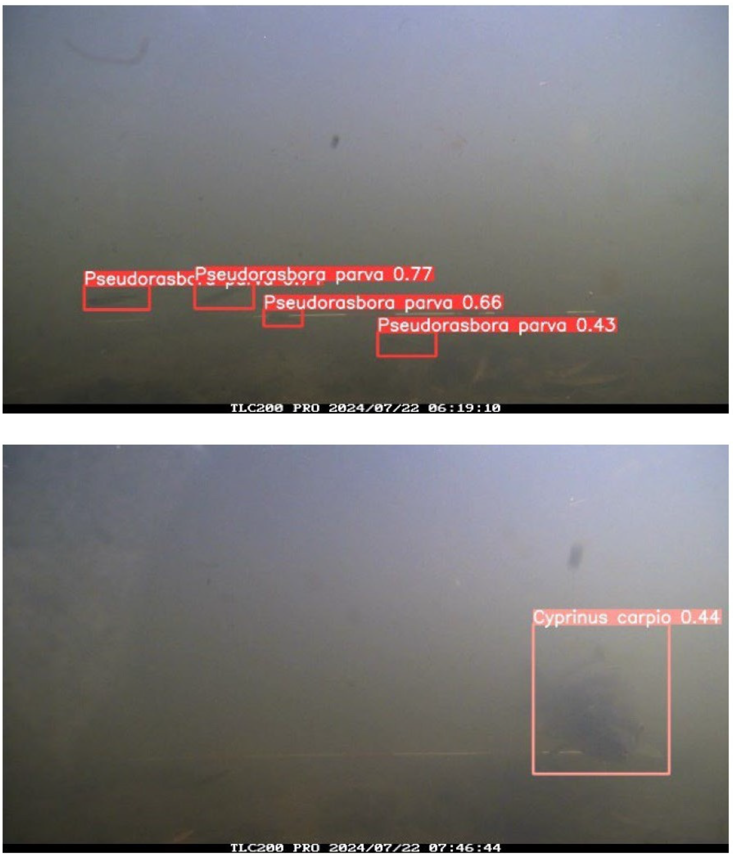
Underwater images were captured at the study site on four occasions: 22 April 2024 from 6:00 to 17:00; 22 July 2024 from 6:00 to 13:00; 26 September 2024 from 6:00 to 17:00; and 18 March 2025 from 7:00 to 16:00. The observation months were selected to cover the period from spring to autumn, when fish activity and movement are relatively high in agricultural drainage canals. Image acquisition was limited to daytime hours to ensure sufficient visibility for reliable detection using optical cameras. The image resolution was 1280 × 720 pixels. The time intervals between images were 2 s on 22 April and 22 July 2024, and 1 s on 26 September 2024, and 18 March 2025. Rainfall was not observed during the monitoring period. Notably, the water depth at the study site was 0.44 m at 6:00 on 22 July, corresponding to the dataset used for inference.

2.3. Dataset

For inferences using the fish detection model, we prepared a dataset consisting of 12,600 images captured between 6:00:00 and 12:59:58 on 22 July 2024. In contrast, the datasets for training and validation were primarily composed of images captured on 22 April, 26 September 2024, and 18 March 2025. However, the data from these three days alone did not sufficiently include images that captured the diverse postures of P. parva and C. carpio or backgrounds that are likely to cause false detections. These variations are crucial for enhancing the ability of the model to generalize and accurately detect the target fish species under different conditions. Therefore, we intentionally included an additional 2.0% of the images from the inference dataset captured on 22 July in the training data so that these critical variations could be adequately represented. This inclusion created a small overlap between the training and inference datasets (approximately 2%), but the impact of this overlap was considered limited, given the small proportion relative to the entire inference dataset (12,600 images). Moreover, the primary objective of this study was not to conduct a general performance evaluation of the object detection model but rather to achieve high accuracy in capturing the occurrence patterns of the target fish species in the drainage canal on a specific day. This focus on practical applicability under real-world conditions directly influenced the manner in which we constructed our datasets.

2.4. Model Training and Validation

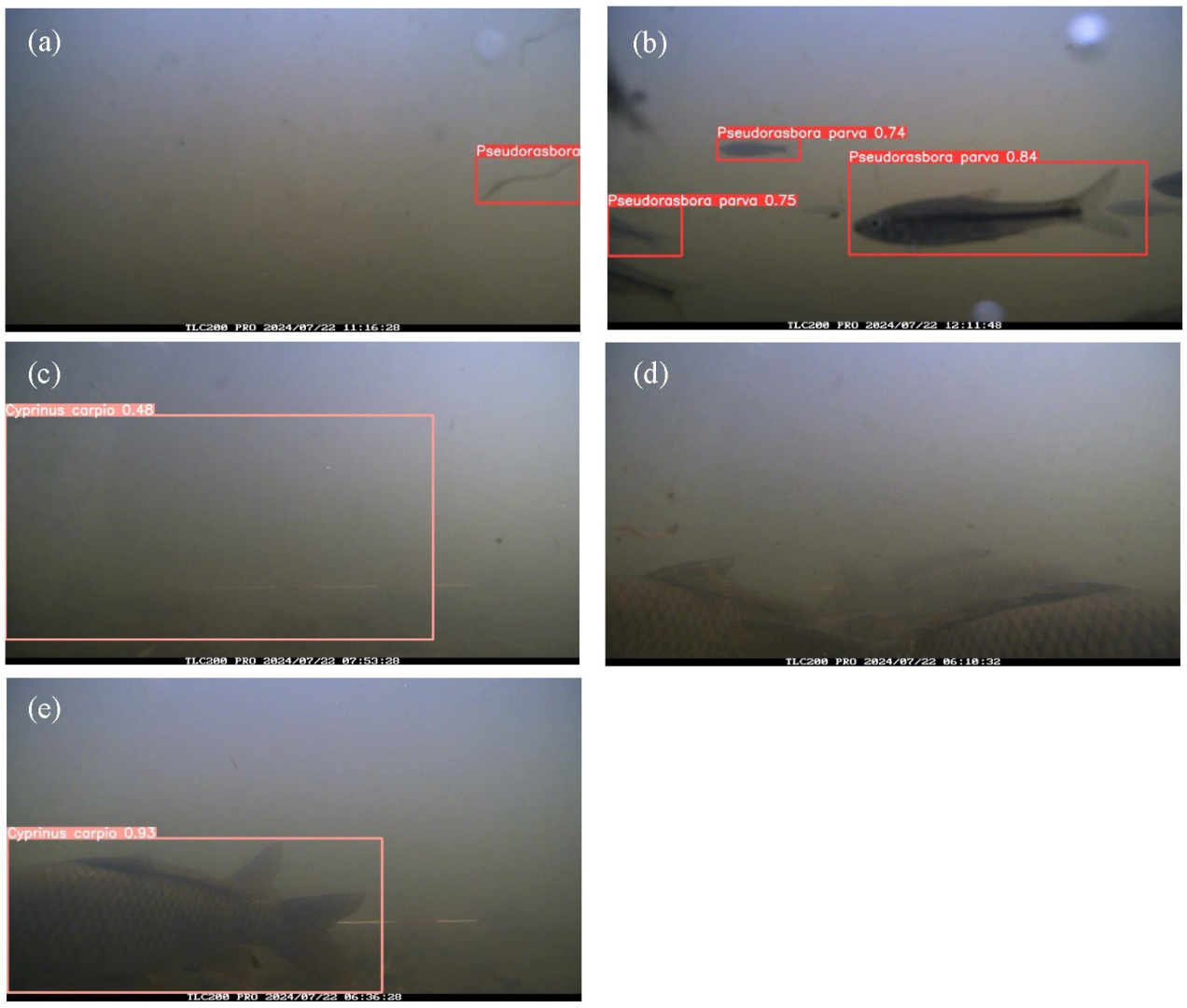
From the four underwater image surveys conducted in this study, we manually identified the presence of several species, including Candidia temminckii (dark chub, “Kawamutsu”), Gymnogobius urotaenia (striped goby, “Ukigori”), Mugil cephalus (flathead grey mullet, “Bora”), Carassius sp. (Japanese crucian carp, “Ginbuna”), Hemibarbus barbus (barbel steed, “Nigoi”), and Neocaridina spp. (freshwater shrimp, “Numaebi”), in addition to Pseudorasbora parva and Cyprinus carpio. Among these, we selected P. parva and C. carpio as the target species because relatively large numbers of individuals were captured in the images. These two species also represent contrasting body sizes, with P. parva being small-bodied and C. carpio being large-bodied, which allowed us to examine differences in detectability. Fish body size and morphological characteristics such as color and shape were important factors influencing detection: smaller species with lower visual contrast against the background (e.g., P. parva) were more prone to missed detections, whereas larger species (e.g., C. carpio) were more reliably detected. Thus, these species were suitable for evaluating the performance of the fish detection model and for estimating temporal distributions of small- and large-bodied swimming fish.

Images containing only non-target organisms were treated as background images and used for training and validation. We prepared the dataset so that both the number of background images and the number of target fish detections maintained an approximate ratio of 4:1 between the training and validation sets. Annotation of P. parva and C. carpio in the images was performed using LabelImg (Ver. 1.8.6) [20]. Individuals were enclosed with rectangles and classified into two classes, with the coordinate information and class IDs saved in YOLO-format text files. An overview of the dataset is provided in

Table 1. Summary of annotated training and validation datasets, including the number of images and fish instances per species.

Category	Training Data	Validation Data
Number of images (total)	546 images	129 images
Number of background-only images	57 images	14 images
Number of images with fish	489 images	115 images
Pseudorasbora parva	305 individuals	76 individuals
Cyprinus carpio	333 individuals	74 individuals

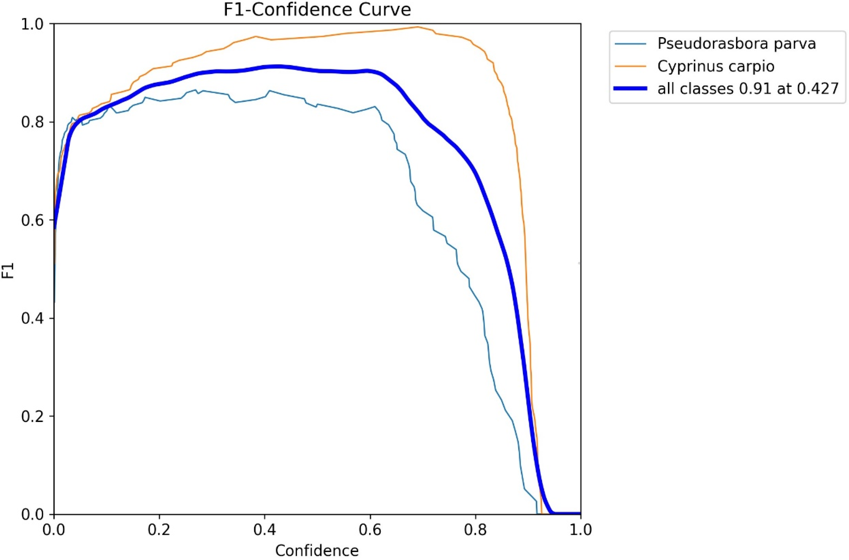
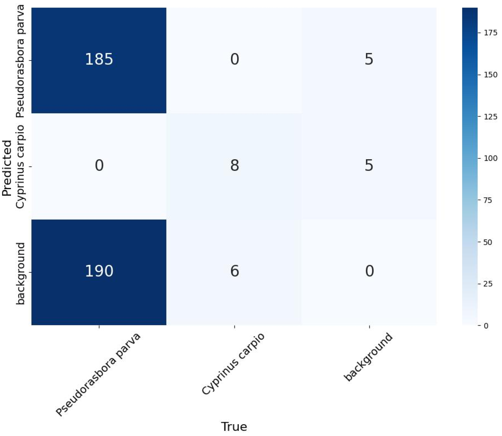
. Background-only frames often contained drifting algae, debris, or other species and were excluded from annotation. The proportion of such background-only images was approximately 10% of the total for both training and validation (Table 1), indicating that nearly 90% of the images were suitable for fish detection and used as valid data for model development. This dataset was selected so that reasonable detection results could be obtained, as confirmed by the Precision–Recall curves, F1–confidence curves, and confusion matrices during validation.

The computational resources and hyperparameters are listed in

Table 2. Computational environment and hyperparameter settings for YOLOv8n training.

Configuration	Parameter
GPU	NVIDIA Quadoro P4000
Operating System	Windows 10 Pro, 64-bit
Python	3.8.5
PyTorch	2.2.0+cu118
CUDA	11.8
Optimizer	AdamW
Initial learning rate	0.001
β1	0.937
β2	0.999
Weight decay	0.0005
Learning rate scheduler	Linear decay
Epochs	500
Input Image Resolution	960 × 960 pixels
Batch Size	16

. We trained the model using a batch size of 16 for 500 epochs, with AdamW as the optimization algorithm for the loss function and an image size of 960 pixels. Following the default settings of YOLOv8, the IoU threshold for assigning positive and negative examples during the matching of the ground truth and predicted boxes was set to 0.2. This threshold balances accuracy and stability and is particularly effective for widening detection candidates when targeting small-bodied fish, such as P. parva, one of the focal species in this study.

During training, YOLOv8n applied several data augmentation techniques by default to enhance generalization and reduce overfitting [21]. Photometric augmentations included random adjustments of hue (±1.5%), saturation (±70%), and value (±40%) in the HSV color space. Geometric augmentations consisted of random scaling (±50%), translation (±10%), and left–right flipping with a probability of 0.5. In addition, mosaic augmentation, which combines four training images into one, was applied consistently. Consequently, although the training dataset consisted of 546 annotated images, the model was effectively exposed to a virtually unlimited number of image variations across epochs, thereby improving robustness under diverse environmental conditions. As a result of this training and validation process, we obtained the best weights that minimized the loss function.

2.5. Methods for Inference and Inference Testing

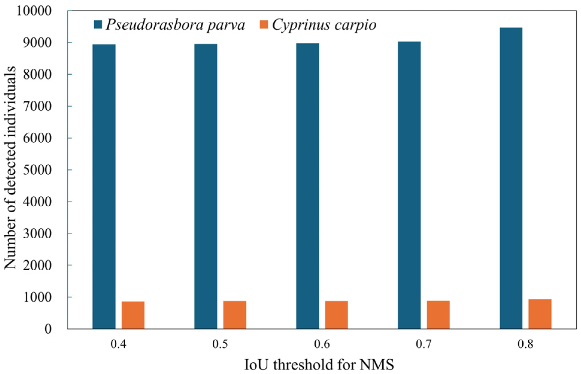
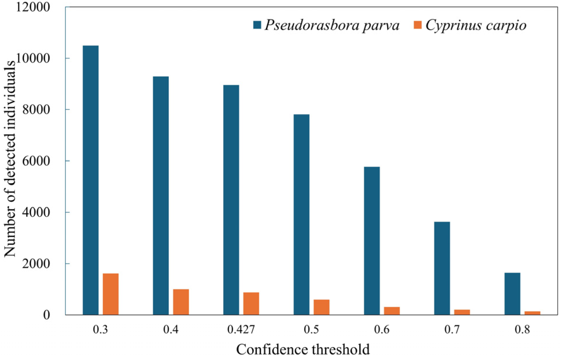
Inference refers to applying the trained model to unlabeled images to estimate fish occurrence, whereas inference testing denotes the evaluation of inference results against manually annotated ground truth data. The best-performing model, obtained through training and validation, was deployed on the inference dataset consisting of 12,600 images. During this inference process, the confidence threshold was explicitly set to the value that maximized the F1-score for both P. parva and C. carpio, as determined from the F1–confidence curves generated during validation. Non-maximum suppression (NMS) was then applied to remove redundant bounding boxes that overlapped on the same object. The IoU threshold for NMS was fixed at 0.5, meaning that when the overlap between two predicted boxes exceeded 50%, only the box with the higher confidence score was retained. This post-processing step ensured that each fish was represented by a single bounding box.

To rigorously assess the reliability and generalization capability of the trained model, we conducted an external validation using held-out data. Specifically, we randomly sampled 300 images from 12,600-image inference dataset to perform a quantitative evaluation. The detection outputs from the model were compared with the manually annotated ground-truth labels created for P. parva and C. carpio using LabelImg. This procedure provides a practical estimate of the detection performance of the model on images not included in the training or validation sets, complementing the internal validation performed during the training phase.

2.6. Estimation of Actual Fish Counts

To estimate the actual number of individual fish that passed through the field of view of the camera during the observation period, we applied a two-step correction to the raw detection counts obtained from the inference dataset. This procedure accounts for (1) undetected individuals owing to imperfect Recall and (2) multiple detections of the same individual across consecutive frames.

First, given the number of detections $N_{\mathrm{detections}}$ and Recall of the model determined from the confusion matrix, the corrected number of occurrences $N_{\mathrm{occurrences}}$ was calculated by compensating for undetected individuals:

$$N_{\mathrm{occurrences}}={\displaystyle \frac{N_{\mathrm{detections}}}{\mathrm{Recall}}}$$

(6)

This correction assumes that detection failures are uniformly distributed and that Recall represents the probability of successfully detecting an individual occurrence.

Second, because a single fish often appeared in multiple consecutive frames, the estimated actual number of individual fish $N_{\mathrm{actual}}$ was obtained by dividing $N_{\mathrm{occurrences}}$ by the average number of detections per individual, denoted as $R_{\mathrm{frames}}$.

$$N_{\mathrm{actual}}={\displaystyle \frac{N_{\mathrm{occurrences}}}{R_{\mathrm{frames}}}}$$

(7)

where $R_{\mathrm{frames}}$ is empirically determined from an analysis of sequential detection images. Based on the patterns observed in this study, $R_{\mathrm{frames}}$ was set to 2.5 for P. parva and 5 for C. carpio.

This approach enabled the estimation of the actual number of individual fish traversing the monitored section of the canal, thereby providing a practical means to quantify fish passages from detection data under field conditions.

3. Results

3.1. Training and Validation

To evaluate the performance of the object detection model (YOLOv8n), we generated an F1-confidence curve using the validation dataset. As shown in Figure 2, the F1 score for both target species peaked at a confidence threshold of 0.427 and was, therefore, selected as the reference value for subsequent analyses, unless otherwise specified.

Table 3. Performance metrics of the YOLOv8n model on the validation dataset, including Precision, Recall, F1 score, and mAP for each fish species.

	Images	Instances	Precision (%)	Recall (%)	F1 Score (%)	mAP50 (%)	mAP50–95 (%)
All species	129	150	95.1	88.4	91.6	95.5	69.0
Pseudorasbora parva	129	76	95.2	78.1	85.8	91.6	58.8
Cyprinus carpio	129	74	95.0	98.6	96.8	99.4	79.1

summarizes the comprehensive evaluation metrics for the model performance on the validation data. For all categories combined, the model achieved a Precision of 95.1%, Recall of 88.4%, F1 score of 91.6%, mAP50 of 95.5%, and mAP50–95 of 69.0%. The performance for C. carpio was particularly high, with a Recall of 98.6% and an F1 score of 96.8%, whereas the Recall for P. parva was relatively low at 78.1%, resulting in an F1 score of 85.8%. Overall, the model demonstrated high accuracy in validation, supporting its potential for reliable fish detection under the given annotation standards and dataset conditions.

3.2. Inference and Inference Testing

To evaluate the performance of the model under more realistic and operational conditions, we computed the detection metrics on 300 randomly sampled images from the inference dataset, which comprised 12,600 images (

Table 4. Detection performance of the YOLOv8n model on 300 randomly selected images from the inference dataset under practical conditions.

	Images	Instances	Precision (%)	Recall (%)	F1 Score (%)	mAP50 (%)	mAP50–95 (%)
All species	300	389	88.9	47.1	61.6	67.8	47.0
Pseudorasbora parva	300	375	96.5	37.0	53.5	72.0	48.7
Cyprinus carpio	300	14	81.2	57.1	67.1	63.6	45.3

). Compared to the internal validation results shown in Table 3, the overall Precision decreased by 6.2% to 88.9%, indicating a modest increase in false positives, whereas the Recall declined substantially by 41.3% to 47.1%, highlighting the increased difficulty of detection under real-world noise and variability.

For individual species, P. parva exhibited very high Precision (96.5%), suggesting a low false positive rate; however, its Recall dropped markedly to 37.0%, indicating a substantial number of missed detections. In contrast, C. carpio achieved a more balanced outcome with a Precision of 81.2% and a Recall of 57.1%, resulting in an F1 score of 67.1%.

Figure 3 shows the confusion matrix derived from the inference results for 300 sampled images. The confidence threshold was set to 0.427, and the IoU threshold for NMS was fixed at 0.5, as described in the previous section.

Examples of successful detections during inference are presented in Figure 4, where all individuals were correctly identified under fixed thresholds (confidence = 0.427, IoU = 0.5). Conversely, Figure 5 illustrates challenging cases, including false positives (for example, floating debris erroneously detected as P. parva) and false negatives (for example, undetected C. carpio), as well as complex scenarios involving overlapping fish and low-light conditions.

Figure 6 and Figure 7 show the sensitivity analyses for the number of individuals detected with respect to the IoU and confidence thresholds, respectively. As shown in Figure 6, the detection counts were largely stable across IoU thresholds ranging from 0.4 to 0.7 for both target species, indicating that detection outcomes are relatively invariant to IoU threshold adjustments within this range. Based on this robustness, an IoU threshold of 0.5 was adopted in subsequent analyses. In Figure 7, varying the confidence threshold resulted in the expected trade-off: increasing the threshold reduced false positives but concurrently elevated the number of false negatives, reflecting the classic Precision–Recall balance inherent to confidence-based detectors.

Figure 8 shows a temporal series of images documenting the entry and exit of two C. carpio individuals within the field of view of the camera, along with the corresponding detection outputs. The thresholds applied were 0.427 for confidence and 0.5 for IoU, offering insights into short-term movement patterns.

Finally, Figure 9 depicts the temporal variation in the 10 min cumulative occurrence counts estimated by the model for (a) P. parva and (b) C. carpio. The IoU threshold is fixed at 0.5. Among the different confidence threshold settings examined, 0.427 for P. parva and 0.7 for C. carpio provided the best agreement with the expected ecological patterns. The black lines in each panel represent the most reliable estimates derived from the analysis. The P. parva appeared frequently during 6:00–7:00, around 10:00, and around 12:00, whereas C. carpio was predominantly observed in the early morning around 6:00.

3.3. Estimated Number of Individuals

Figure 7 shows the variation in the number of detected individuals across different confidence thresholds, with the IoU threshold fixed at 0.5. For P. parva, the number of detections decreased sharply as the confidence threshold increased from 0.427 to 0.5, which is consistent with the F1-confidence curve in Figure 2, where the F1 score peaked at approximately 0.42.

As illustrated in Figure 4, most detection confidence scores for P. parva were concentrated between 0.4 and 0.7. Considering that the underwater images were generally turbid and only captured clear outlines when the fish were close to the camera (Figure 5), high-confidence detection was less common for small, indistinct species, such as P. parva.

The confusion matrix in Figure 3, with a confidence threshold of 0.427, indicated 185 true positives (TP) and 190 false negatives (FN) for P. parva, corresponding to a Recall of approximately 0.49. Accordingly, the total number of occurrences can be estimated by correcting for Recall using

$$N_{\mathrm{occurrences}}={\displaystyle \frac{N_{\mathrm{detections}}}{\mathrm{Recall}}}={\displaystyle \frac{9000}{0.49}}\approx \mathrm{18,367}$$

(8)

Applying this to 9000 detections at this threshold yielded approximately 18,367 occurrences. Additionally, based on the analysis of sequential frames (Figure 8), each individual P. parva was estimated to be detected approximately 2.5 times on average. Thus, the actual number of individuals is given by

$$N_{\mathrm{actual}}={\displaystyle \frac{N_{\mathrm{occurrences}}}{R_{\mathrm{frames}}}}={\displaystyle \frac{\mathrm{18,367}}{2.5}}\approx 7347$$

(9)

Therefore, it was estimated that approximately 7300 individual P. parva passed through the field of view between 6:00:00 and 12:59:58 on 22 July 2024.

A similar estimation was made for C. carpio. As shown in Figure 2, the F1 score for C. carpio peaked at a confidence level of 0.69. Therefore, a threshold of 0.7 was adopted. At this threshold, there were 204 detections, with a Recall of 0.5. This gives:

$$N_{\mathrm{occurrences}}={\displaystyle \frac{204}{0.5}}=408$$

(10)

Considering that each C. carpio individual was typically detected in approximately five consecutive frames (approximately 10 s), as shown in Figure 8, the estimated number of individuals was

$$N_{\mathrm{actual}}={\displaystyle \frac{408}{5}}\approx 82$$

(11)

Hence, approximately 80 individual C. carpio are estimated to have passed through the field of view of the camera during the same period.

4. Discussion

This study demonstrated the applicability of a state-of-the-art deep learning model, YOLOv8n, for fish detection in agricultural drainage canals. The model was applied to an inference dataset consisting of 12,600 images, and the results showed that fish occurrence patterns in this complex environment could be effectively captured. The performance evaluation during validation confirmed that the model achieved sufficiently high precision, recall, and mAP values, supporting the feasibility of using deep learning for ecosystem monitoring in rural waterways. Importantly, this study provides one of the first applications of a modern object detection model to agricultural drainage canals, thereby offering a novel approach for monitoring freshwater biodiversity in agricultural landscapes.

Notably, variation in detection performance within the 7 h observation period was influenced by short-term environmental conditions rather than seasonal differences. During the monitoring on 22 July, no rainfall was recorded, but intermittent cloud cover caused temporal fluctuations in brightness, reducing image contrast in some periods. In addition, sediment resuspension occurred when C. carpio moved across the canal bed, temporarily increasing turbidity and reducing visibility. These factors explain why recall was lower in certain situations, even though water clarity did not vary markedly at the daily scale. Clarifying these influences strengthens the ecological interpretation of our results.

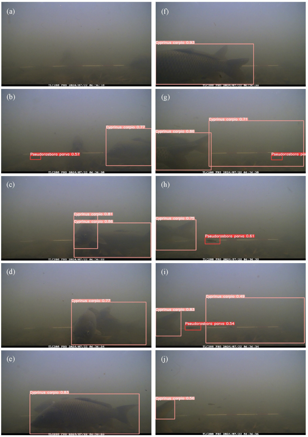
Detection performance also differed between the two target species. For the small-bodied P. parva, recall was reduced because individuals were difficult to detect under turbid conditions and often blended with the background. In contrast, for the large-bodied C. carpio, precision was comparatively lower (81.2%) because large turbid plumes or debris clouds generated during carp movements were occasionally misidentified as carp. These results indicate that the main source of detection errors differed between the two species: missed detections were more frequent for small-bodied fish, whereas false positives were more common for large-bodied fish. Although performance was not optimal, the method still produced ecologically meaningful estimates (approximately 7300 P. parva and 80 C. carpio over 7 h), demonstrating the feasibility of deep learning-based non-invasive monitoring in agricultural waterways.

Previous research has highlighted the potential of deep learning for fish detection under various conditions. For example, Jahanbakht et al. [7] proposed a semi-supervised and weakly supervised deep neural network for binary fish classification in turbid marine environments. However, their dataset consisted of weak labels (fish present/absent), and detailed annotations with bounding boxes were not provided. Vijayalakshmi and Sasithradevi [9] developed AquaYOLO, an advanced YOLO-based architecture for aquaculture pond monitoring, demonstrating improved performance in controlled environments. Compared to these studies, our work focused on a more challenging setting: agricultural drainage canals, where turbidity is compounded by drifting filamentous algae, fallen leaves, and branches. The use of frame-level annotations with bounding boxes and species labels (P. parva and C. carpio) ensured reliable evaluation of model performance in these highly variable inland waters.

A methodological distinction also exists between our study and previous work. Kandimalla et al. [10] randomly divided their dataset into training (80%) and test (20%) subsets, using the test set exclusively to evaluate model accuracy. This is a standard approach in machine learning research. In contrast, the present study aimed to analyze the entire inference dataset of 12,600 images in order to examine temporal patterns of fish occurrence in agricultural drainage canals. To ensure the reliability of this large-scale inference, 300 images were randomly sampled from the inference dataset, manually annotated, and compared with the inference results. Thus, the role of inference testing in our study was different: rather than serving as a conventional test split, it functioned as a credibility check for full-scale inference applied to all available data. This design reflects the applied nature of our research, where the objective was not only to evaluate the model but also to generate ecologically meaningful information from the entire dataset.

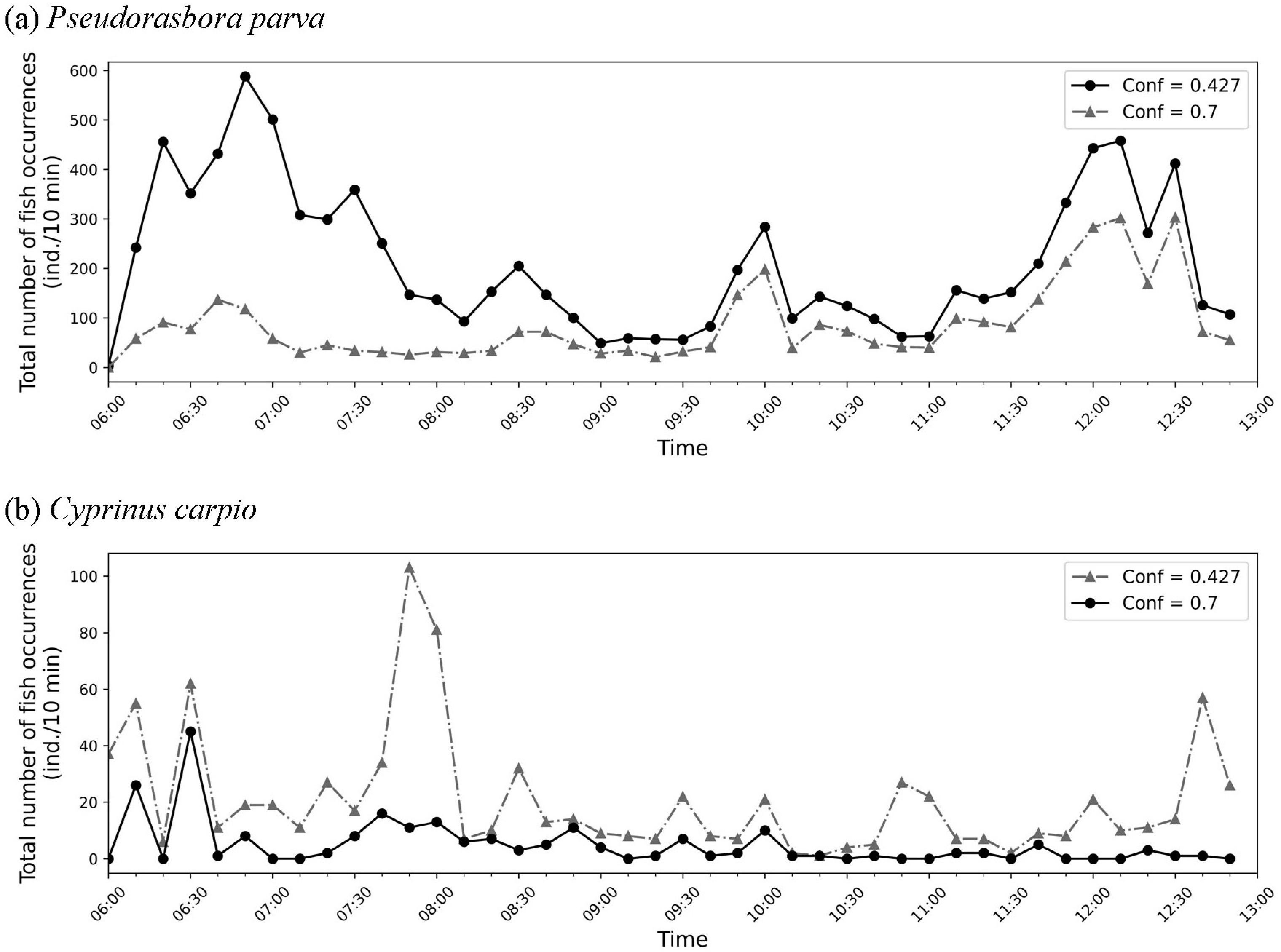
The time-series analysis of fish occurrence in this study conceptually corresponds to the outputs of Liu et al. [15], who visualized hourly variations in fish abundance in a marine ranching environment. Both approaches highlight temporal patterns of fish activity by summarizing occurrence counts within fixed time intervals. However, while Liu et al. [15] focused on large-scale aquaculture and employed a multi-class detection-and-tracking framework, our study targeted freshwater fish in agricultural drainage canals and analyzed occurrence counts per 10 min intervals using YOLOv8n with inference testing. These differences underscore the novelty of our work, which extends deep learning-based fish monitoring from aquaculture contexts to agricultural waterways, thereby broadening its applicability to ecohydraulic management and biodiversity conservation. Although the recall of our trained model was limited, particularly for C. carpio, the relatively high precision (81.2% for C. carpio and 95.1% for P. parva) ensured that most of the detections were correct. As a result, while the absolute number of fish occurrences may be underestimated due to missed detections, the time series analysis of occurrence frequency remains meaningful as a reference for identifying relative fluctuations and temporal patterns in fish activity. This highlights that deep learning-based monitoring can still provide ecologically relevant insights, even under challenging field conditions.

Despite the promising results obtained in this study, several limitations remain that point to directions for future research. The training dataset was relatively small, and additional annotated images covering diverse environmental conditions would likely improve model robustness. Moreover, this study focused solely on object detection, without incorporating tracking or behavior analysis, which could provide deeper ecological insights. Future work should also consider advanced inference techniques for small object detection. For example, Akyon et al. [22] proposed the Slicing-Aided Hyper Inference (SAHI) framework, which improves detection accuracy by slicing large images into patches during inference and aggregating the results. Since the target species in this study often occupy only a small pixel area in underwater images, applying SAHI could further enhance the recall of fish detection in agricultural drainage canals.

Although the number of manually annotated images in this study was relatively small compared with typical machine learning benchmarks, reliable estimates of fish occurrence were still achieved. This outcome was partly due to the application of data augmentation, which increased variability and enhanced the generalization of the trained model. From a practical standpoint, demonstrating the effectiveness of a model trained with a limited number of annotated images is particularly important, because large-scale annotation is highly labor-intensive and may discourage widespread adoption of deep learning techniques in ecological monitoring. Therefore, the ability to obtain ecologically meaningful outputs with relatively few annotations highlights the practical value of our approach. Nonetheless, expanding annotated datasets across different canals and under diverse environmental conditions remains an important future direction to further strengthen model robustness.

5. Conclusions

This study demonstrated the applicability of a state-of-the-art deep learning model (YOLOv8n) for monitoring fish occurrence in agricultural drainage canals. Using 12,600 underwater images collected over a 7 h period, the model detected two representative species, Pseudorasbora parva and Cyprinus carpio, and estimated that approximately 7300 and 80 individuals, respectively, passed the observation site. These results confirm that deep learning provides a non-invasive and effective method for quantifying temporal fish occurrence in turbid and dynamic inland waterways. The novelty of this work lies in applying modern object detection to an ecologically significant yet technically challenging environment, thereby extending the use of deep learning from aquaculture and marine contexts to agricultural landscapes. Future work should expand annotated datasets and adopt advanced inference techniques to improve recall for small-bodied species and under low-visibility conditions.