Article

Active Distribution Network Bi-Level Programming Model Based on Hybrid Whale Optimization Algorithm

Key Laboratory of Smart Grid of Ministry of Education, Tianjin University, Nankai District, Tianjin 300072, China
*
Author to whom correspondence should be addressed.
Sustainability 2025, 17(19), 8560; https://doi.org/10.3390/su17198560
Submission received: 18 July 2025 / Revised: 7 August 2025 / Accepted: 18 August 2025 / Published: 24 September 2025

Abstract

In recent years, the integration of flexible resources into active distribution networks (ADNs) has been significantly enhanced. By coordinating a variety of such resources, the economic efficiency, operational security, and overall stability of ADNs can be improved. In this study, a bi-level planning model is proposed for active distribution networks. The upper-level model aims to minimize the annual comprehensive cost, while the lower-level model focuses on reducing network losses. To solve the upper-level problem, a hybrid whale optimization algorithm (HWOA) is developed. The algorithm integrates adaptive mutation based on Gaussian–Cauchy distributions, a nonlinear cosine-based control strategy, and a dual-population co-evolution mechanism. These enhancements allow HWOA to achieve faster convergence, higher accuracy, and stronger global search capabilities, thereby reducing the risk of falling into local optima. The lower-level problem is addressed using the interior point method due to its nonlinear and continuous nature. The proposed model and algorithm are validated through simulations on the IEEE 33-bus system. The results show that DG consumption increases by 88.77 MWh, network losses decrease by 6.8 MWh, and the total system cost is reduced by CNY 3.62 million over the entire project lifecycle. These improvements contribute to both the economic and operational performance of the ADN. Compared with the polar fox optimization algorithm (PFA), HWOA improves algorithmic efficiency by 18.92%, lowers network loss costs by 6.22%, and reduces the total system costs by 0.71%, demonstrating its superior effectiveness in solving complex bi-level optimization problems in active distribution networks. These findings not only demonstrate the technical efficiency of the proposed method but also contribute to the long-term goals of sustainable energy systems by improving renewable energy utilization, reducing operational losses, and supporting carbon reduction targets in active distribution networks.

1. Introduction

In recent years, the construction of new power systems has been actively promoted in many countries. These efforts have been driven by the rapid development of renewable energy and the growing urgency of carbon neutrality targets. In China, the “dual carbon” policy—aiming for carbon peaking by 2030 and carbon neutrality by 2060—has provided strong momentum for power system reform. At the same time, a large number of distributed energy resources have been deployed at the distribution level. The installed capacity of distributed photovoltaic systems in China exceeded 160 GW by the end of 2023. This trend is expected to continue. As a result, higher requirements have been placed on the flexibility, observability, and controllability of distribution networks. In response to these changes, the concept of the ADN has been proposed. ADNs are characterized by multi-source coordination, dynamic regulation, and intelligent interaction. Their planning and operation must consider multiple types of resources, including distributed generation, demand-side management, and grid infrastructure. In particular, flexible regulatory resources such as demand response (DR) have been increasingly integrated into ADNs. By coordinating these resources effectively, the economic efficiency and operational stability of the grid can be improved. Therefore, the collaborative planning of source, network, and load has become a key research focus under the new power system paradigm [1].
Simultaneously, a diversification of adaptable regulatory resources has been observed, along with increasingly varied electricity demand patterns from grid users. As a result, the traditional distribution network has been gradually transformed into an ADN, which is characterized by multiple power sources, enhanced observability and controllability, as well as improved capabilities for active coordination and optimized management [2]. In the context of the new power system environment, a wide range of adjustable resources exists within the ADN. If these resources are planned and coordinated in a collaborative and integrated manner, significant improvements in both economic efficiency and grid stability can be achieved. Given the numerous challenges arising under the new power system paradigm, the collaborative planning of source, network, and load has become increasingly critical.
Recent studies on ADN planning have mainly focused on two aspects: model development and algorithm design. In terms of model structure, most existing works can be categorized into single-level models and bi-level programming models (BPMs).
Single-level planning models have been widely applied due to their simplicity and computational efficiency. For instance, a multi-objective ADN model based on uncertain stochastic networks was proposed in ref. [3]. In ref. [4], a two-stage robust model was developed for siting of EV charging stations under uncertain load and generation conditions. However, these models often fail to reflect the hierarchical decision-making process between long-term planning and short-term operation. A multi-stage planning approach considering DG and DR uncertainties was proposed in ref. [5], but the interaction between source, network, and load components remains limited.
To overcome these limitations, bi-level models have been introduced to separately handle planning and operation decisions. For example, a BPM considering wind power uncertainty was established in ref. [6], but DR was not incorporated. In ref. [7], unit operating constraints under renewable uncertainty were considered, yet DR was again omitted. A more comprehensive BPM with DR was proposed in ref. [8], though the modeling of source–network–load interaction still requires further improvement.
On the algorithmic side, intelligent optimization methods have been extensively adopted to solve ADN planning problems. Particle swarm optimization was applied in refs. [9,10,11], while genetic algorithms were used in refs. [12,13,14,15], grey wolf optimization appeared in refs. [16,17], and so on. The advantages and disadvantages of the planning results depend on the performance of intelligent algorithms. Compared to alternative intelligent algorithms, the whale optimization algorithm (WOA) possesses advantages such as a straightforward structure, strong adaptability, and rapid convergence speed. However, the basic WOA also presents several limitations, including low population diversity, excessive reliance on the current optimal individual, a singular population search strategy, and weak local search capabilities, which can lead to premature convergence and entrapment in local optima.
To address the collaborative planning problem in ADNs, a bi-level programming model (ADN-BPM) is established. The effects of distributed generation and DR are carefully considered in the model design. The upper-level planning model is formulated to minimize the annual comprehensive cost, while the lower-level model is designed to reduce network losses. The lower-level problem is solved using the interior point method due to its continuous and nonlinear nature. For the upper-level problem, a hybrid improved whale optimization algorithm is proposed. This algorithm incorporates an adaptive mutation mechanism, a nonlinear control factor based on a cosine function, and a dual-swarm co-evolution strategy. The effectiveness of the proposed model and algorithm is verified through simulations based on the IEEE 33-bus test system.
The main innovative contributions of this study are as follows:
  • Demand response is introduced into the ADN planning problem to realize “source-load-network” collaborative planning, which can effectively reduce the network loss and cost of the system.
  • A hybrid improved whale algorithm is proposed to optimize the algorithm structure and search method of the whale algorithm through co-evolution and adaptive mutation, which effectively improves its convergence speed and optimization accuracy.

2. ADN “Source-Load-Network” Two-Tier Planning Model

Figure 1 presents the ADN “source-load-network” two-tier planning model investigated in this study. Unlike conventional approaches, demand response (DR) is integrated into the investment planning stage in the proposed upper-level model. Through this integration, a more adaptive allocation of resources is achieved. In addition, a coordinated mechanism between planning decisions and demand-side flexibility is established.

2.1. Upper-Level Planning Model

2.1.1. Objective Function

The upper layer is the planning layer, which makes decisions on the siting and capacity setting of the DG in terms of economics to achieve the goal of minimizing the total cost of the system, with the following objective function:
C all   = C inv   + C m + C buy + C loss   + C DR + C E s s
C inv = c inv i = 1 N i C a DG i r 1 + r y 1 + r y 1
C m = 365 t = 1 N t i = 1 N i c m P DG i , t
C buy = 365 t = 1 N t c buy t P buy t
C loss   = 365 t = 1 N t c loss P loss t
C DR = 365 t = 1 N t j = 1 N DR   c DR t , j P DR t , j
C E S S = 365 t = 1 N t m e s s P e s s t
where C all   is the total system cost; the annual investment cost is denoted as C inv ; the annual operation and maintenance (O&M) cost is represented by C m ; the cost of purchasing power from the higher level is expressed as C s ; the annual network loss cost is indicated by C lass ; the cost of compensating interruptible loads is defined as C DR ; c inv is the investment cost per unit capacity of DG; C E S S is the energy storage cost; N i represents the number of nodes to be connected by the DG; C a DG i signifies the capacity of the DG; r and y stand for the discount rate and the lifecycle of the DG; N t is the total number of time slots in a day; P DG i , t denotes the actual output of the DG during the time slot; c m represents the operating cost per unit of the DG; P buy t and c buy t correspond to the transmission power and the tariff of the purchased power during the time slot; P loss t is the network loss at the time; c loss is the network loss tariff; N DR is the quantity of consumers on the demand side; P k , l DR , j and c DR t , j are the electricity consumption and compensation tariff of the j th consumer at t time, respectively; m e s s is the operation and maintenance cost coefficient per unit power of the energy storage system; P e s s t is the charging and discharging power at the time [18].

2.1.2. Constraints

DG’s access capacity constraint is as follows:
0 S i S i , max
where the maximum access capacity of the DG is determined as S i , max .

2.2. Lower-Level Planning Model

2.2.1. Objective Function

The operation layer, situated at the lower stratum, strives to optimize the system’s operational state through the coordination of DG and DR’s actual output control. The objective is to minimize network loss, with the corresponding expression as the optimization criterion.
P loss = t = 1 N t i , j Ω I i j t 2 R i j
where I i j t is the branch current between node i and node j at the time of t , and R i j is the branch resistance between node i and node j .

2.2.2. Constraints

The lower-level optimization model considers the operational state of the system and satisfies the following constraints:
(i)
Equation constraints
(1) Power balance constraints
P i t = U i t j i U j t G i j cos θ i j + B i j sin θ i j Q i t = U i t j i U j t G i j cos θ i j B i j sin θ i j
where P i t and Q i t denote the active and reactive power values of node i ; U i , t and U j , t are the voltage magnitudes of node i and node j , respectively; G i j and B i j are the conductance of node i and node j ; and θ i j is the phase angle difference between node i and node j .
(2) Node voltage constraints
U i t 2 = U i t 2 + 2 r i j P i j t + x i j Q i j t r i j 2 + x i j 2 I i j t 2
where U i t and U j t denote the voltage amplitude at nodes i and j , respectively, and r i j and x i j are the impedances between node i and node j .
(3) Branch current constraints
I i j t 2 = P i j t 2 + Q i j t 2 U i t 2
(ii)
Inequality constraints
(1) Node voltage amplitude constraints
U i min U i , t U i max
where U i max and U i min denote the upper and lower voltage limits of the node i , respectively.
(2) Node harmonic distortion constraints
h = 2 H ( U i , t h ) U i 1 T H D +
where U i h denotes the amplitude of the h -th order voltage harmonic at the node i ; T H D + denotes harmonic limit of the node i ; H denotes the highest order of voltage harmonics.
(3) Branch circuit capacity constraints
L i j L i j max
where L i j denotes the capacity of the line between node i and node j ; L j max denotes the rated capacity of the line between node i and node j .
(4) DG operational constraints
0 P DG i , t min ( P DG , max i , t , P rated , max i , t )
(5) Reliability constraint
S A I D I S A I D I max S A I F I S A I F I max
where S A I D I denotes the average outage duration per customer per year; S A I F I denotes the average number of outages per customer per year; S A I D I max and S A I F I max denote the limits of system reliability [19,20].

3. Hybrid Whale Optimization Algorithm

3.1. Basic WOA

WOA mimics the unique hunting style of whales, simulating the way humpback whales search, encircle, and catch prey during the search for superiority for position updates.

3.1.1. Whale Encircling Prey Stage

When the whales start to carry out feeding activities, because it is not possible to determine the specific location of the prey in advance, the WOA assumes that the current feeding position is the best feeding position, and then the rest of the individuals approach the best position and carry out the position update. The mathematical model of its position update is:
D = C X * t X t
X t + 1 = X * t A D
where D represents the distance between the current whale and the whale in the optimal position; X * t is the current position of the best individual; X t indicates the current individual position; and t indicates the number of iterations.
The coefficient vectors A and C to control the way the whale swims can be obtained from the following equation:
A = 2 a r a
C = 2 r
where r is a random number in the interval 0 ,   1 and a is a linearly decreasing vector with the following expression:
a = 2 2 t T max
where T max is the maximum number of iterations.

3.1.2. Stages of the Bubble Web Attack

When an individual whale discovers its prey, it will move through a spiral motion to round up the prey and, in the process, constantly update its position and that of the prey.
X ( t + 1 ) = D e s l cos ( 2 π l ) + X * ( t )
D = X * ( t ) X ( t )
During the process of rounding up prey, groups of whales move in a spiral motion to close the distance between them and their prey. The process can be represented as:
X ( t + 1 ) = X * ( t ) A D , p < 0.5 D e s l cos ( 2 π l ) + X * ( t ) , p 0.5
where D is the value of the distance between the position of an individual whale and the optimal solution; s denotes a constant in the shape of a logarithmic spiral; l is a random vector at [ 0 ,   1 ] ; and p is a random value within [ 0 , 1 ] .

3.1.3. Search and Predation Phase

When A is not less than 1, it means that the whale is foraging randomly in the global space. The distance value D is updated randomly, which can enhance the foraging ability. The mathematical model of the scheme is presented as:
D = C X r a n d X
X t + 1 = X r a n d A D
where X r a n d is a vector of randomized locations of individuals selected from the current population.

3.2. Improvement in WOA

The performance of the WOA has been limited by several inherent shortcomings when applied to complex optimization problems. To address these issues, an HWOA is proposed in this study. The algorithmic structure and search strategy of the original WOA have been improved accordingly.

3.2.1. Optimization of Algorithm Structure Based on Co-Evolution

As for the algorithm structure, this study introduces the idea of co-evolution to optimize the population updating mechanism of the traditional WOA and proposes a two-flock co-evolutionary strategy [21]. The strategy first divides the gull flock into elite gulls and common gulls according to the fitness value, in which the proportion of elite gulls is controlled by the parameter R e l i t e .
During the iterative process, the elite wolves use local search to explore locally by performing small spiral movements at the original position, while the regular wolves continue to use the position update formula of the original algorithm. The update formula for the elite wolf position P o s E i is:
P o s E i ( t + 1 ) = P o s S i ( t ) × x × y × z
The update formula for the common gull location P o s S i is:
P o s S i ( t + 1 ) = D i s ( t ) × x × y × z + P o s best   ( t )
A more refined approach involves the adoption of a dual-cluster co-evolutionary strategy, effectively enhancing the equilibrium between local and global search capabilities. This enables HWOA to achieve superior optimization performance and convergence behavior compared to the original WOA.
The control factor k c plays a role in balancing global exploration and local exploitation. Therefore, to address the problem of mismatch between the linear variation in k c and the actual search situation, this study introduces an improved method based on the cosine function to adjust the variation in k c in the same way as ref. [22]. The cosine function has better smoothness and periodicity in the periodic change, which will help to make the change in the control factor smoother and better adapt to the search process of the population. The improved control factor expression is:
k c ( t ) = k max k max k min × cos π t 2 T max π 2
where k c ( t ) denotes the control factor of the WOA at the t -th iteration, k max   is the maximum value of the control factor, and k min   is the minimum value of the control factor.

3.2.2. Optimization of Search Method Based on Adaptive Mutation

As for the search method, this study proposes an adaptive variant WOA strategy based on the combination of Gaussian variation and Cauchy variation to enrich the search method of the population. Among them, the formula of Gaussian variation operation is as follows [23]:
P i G = P i 1 + Gauss 0 , σ 2
where P i G denotes the position after the Gaussian variation operation; P i is the position before the variation; Gauss 0 , σ 2 is the Gaussian variation operator, whose function is to generate a random number obeying a standard normal distribution.
The formula for the Cauchy variation operation is as follows:
P i C = P i ( 1 + Cauchy ( 0 , ρ ) )
where P i C denotes the position after the Cauchy variation operation; Cauchy ( 0 , ρ ) is the Cauchy variation operator, which serves to generate a random number that obeys the standard Cauchy distribution.
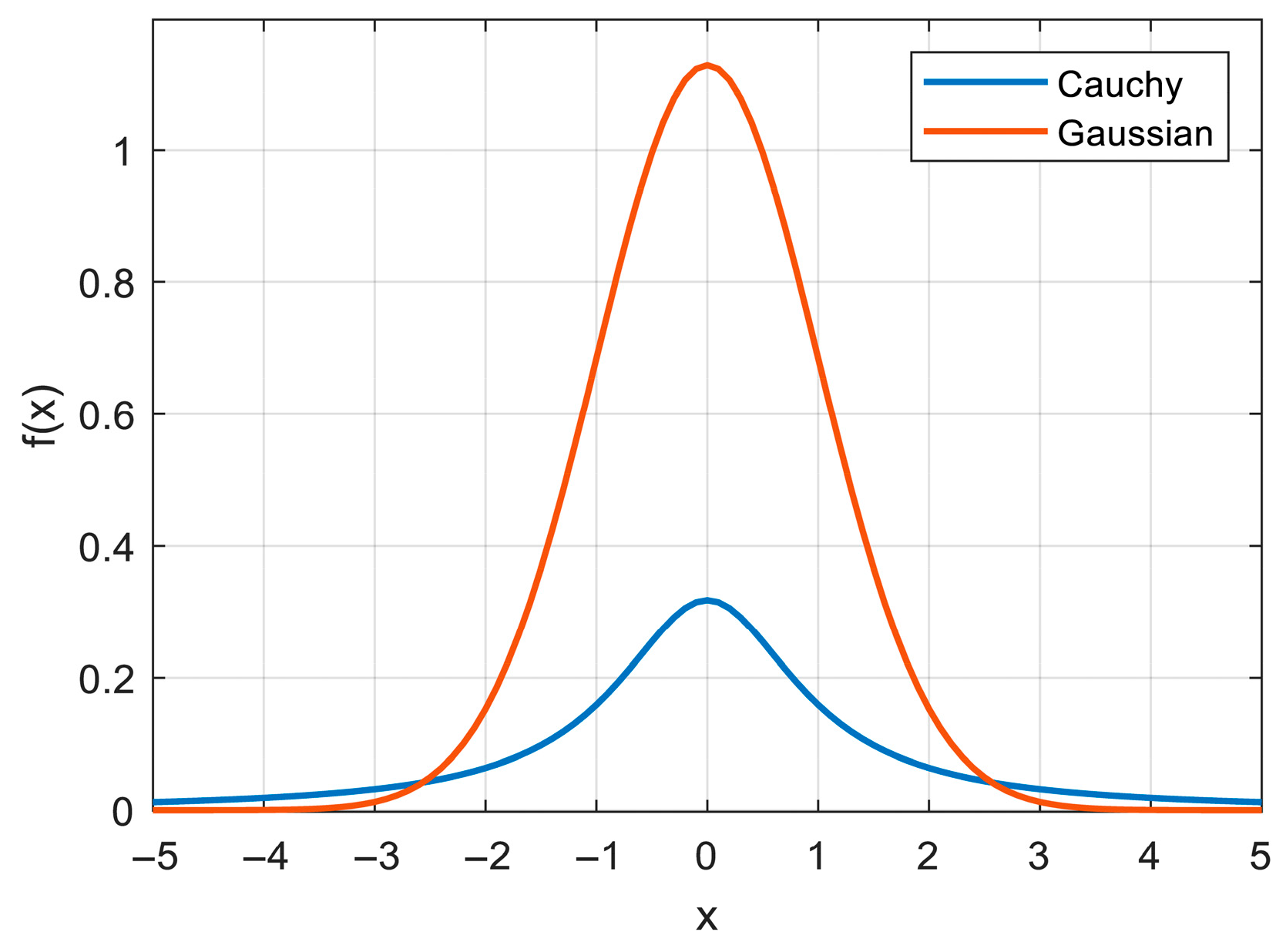
Figure 2 illustrates the standard normal distribution curve alongside the standard Cauchy distribution curve, indicating that the Gaussian variant exhibits a more robust local search capability while demonstrating a comparatively weaker global search capability. The Cauchy variant, on the other hand, has a better global search ability due to its wider distribution range, and it is easier to jump out of the local traps.
According to the different advantageous characteristics of the Cauchy and Gaussian variants, this study combines these two variants and introduces an adaptive variational strategy, which acts on the optimal wolf based on Section 2.2.1:
P o s best . V ( t ) = α P o s best ( t ) α = [ 1 + γ Cauchy ( 0 , 1 ) + ( 1 γ ) Gauss ( 0 , 1 ) ]
where P o s best . V   ( t ) denotes the location of the optimal gull after mutation; Cauchy ( 0 , 1 ) and Gauss ( 0 , 1 ) are the standard Gaussian and standard Cauchy variants, respectively; γ = 1 t 2 / m a x I t e r 2 is the coefficient of control of the variance. The adaptive adjustment of γ occurs in accordance with the number of iterations, allowing the algorithm to emphasize global exploration in the initial stages and local refinement in the subsequent phases. The adaptive adjustment of control parameters enables better global exploration in early iterations and improved local refinement later. As a result, HWOA achieves higher accuracy and avoids local optima more effectively than the original WOA.
The mutated position is not necessarily better than the original position, and a greedy selection strategy is needed to define a good evolutionary direction for the optimal wolf, whose position update formula is:
H S best   ( t + 1 ) = H S best .   V ( t ) ,   if   f H S best . ( t ) < f H S best   ( t ) H S best   ( t ) ,   otherwise  
The flow of the HWOA is as follows:
  • The algorithm parameters were set according to Equations (19) and (20) to randomly generate the initial population;
  • The initial population fitness values were calculated and ranked to mark the optimal individuals;
  • Flocks of gulls were categorized into elite and common gull flocks based on sorting, with the proportion of elites generated by a feedback-adjusted formula;
  • The control factors were updated according to the cosine control strategy of Equation (30);
  • Updating elite gulls, establish common gull positions according to the dual-flock co-evolution strategy;
  • The ranking of the gull flock is updated, and the optimal individuals are determined by calculating the fitness value of the new population using Equations (21)–(29);
  • Mutation and update operations are performed on the optimal individuals according to Equations (33) and (34);
  • Check if the maximum iteration limit has been reached; if so, cease iteration and output the optimal value. Otherwise, proceed to step 3 to resume iteration.

3.3. Model Solving Process

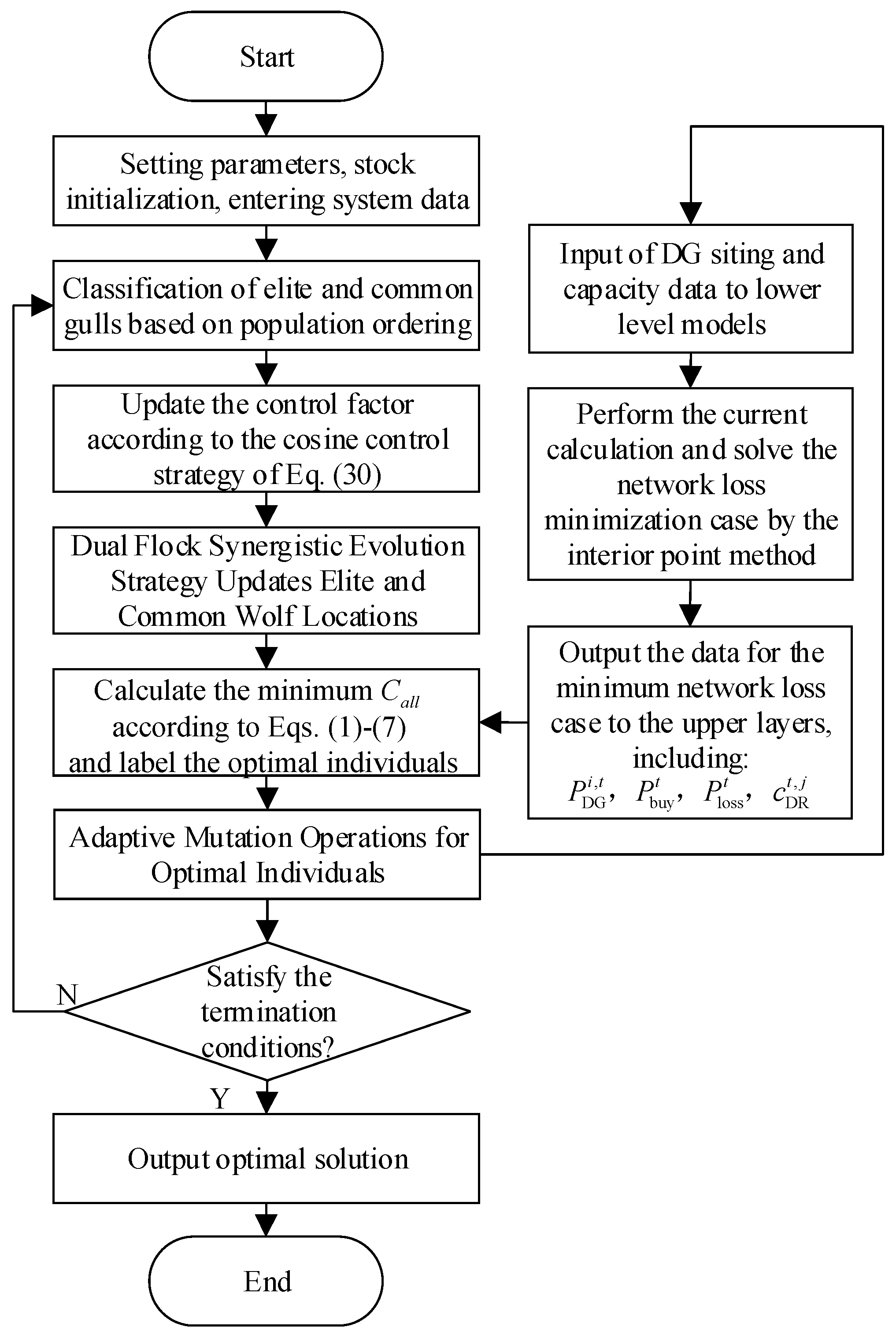
In addressing the ADN “source-network-load-storage” planning issue, the upper-layer model is employed predominantly for optimizing and addressing the DG planning problem. The control variables within this model are entirely discrete. In contrast, the lower-layer model is primarily utilized for optimizing and resolving the operational state of the distribution network, constituting a nonlinear model. Consequently, the upper layer is addressed through the novel HWOA introduced in this study, while the lower layer is tackled using the interior point method. A schematic representation of the solution process is depicted in Figure 3.
In terms of constraint handling, the fitness of the overrun results is improved using a penalty function to exclude them.

4. Example Analysis

4.1. Parameterization

The ADN two-layer planning model and HWOA proposed in this study are subjected to simulation and analysis using the IEEE 33-node distribution network arithmetic example. The system data, as referenced in ref. [24], along with the typical daily load and DG output data, as referenced in ref. [25], are employed. Three DG access points are designated, each with an individual DG capacity upper limit of 1500 kVA. The various economic indices of the system are presented in Table 1. All simulations were conducted on a Windows 10 system using MATLAB R2021b.
The parameters of each algorithm are set as followed: The control factor fc of the WOA is set to linearly decrease from 2, while the control factor fc of the HWOA algorithm is set to nonlinearly decrease from 2, with a fixed elite ratio Relite = 0.5. The population size N for each algorithm is established at 50, with the maximum allowed number of iterations, T max , also set to 50.

4.2. Algorithm Performance Analysis

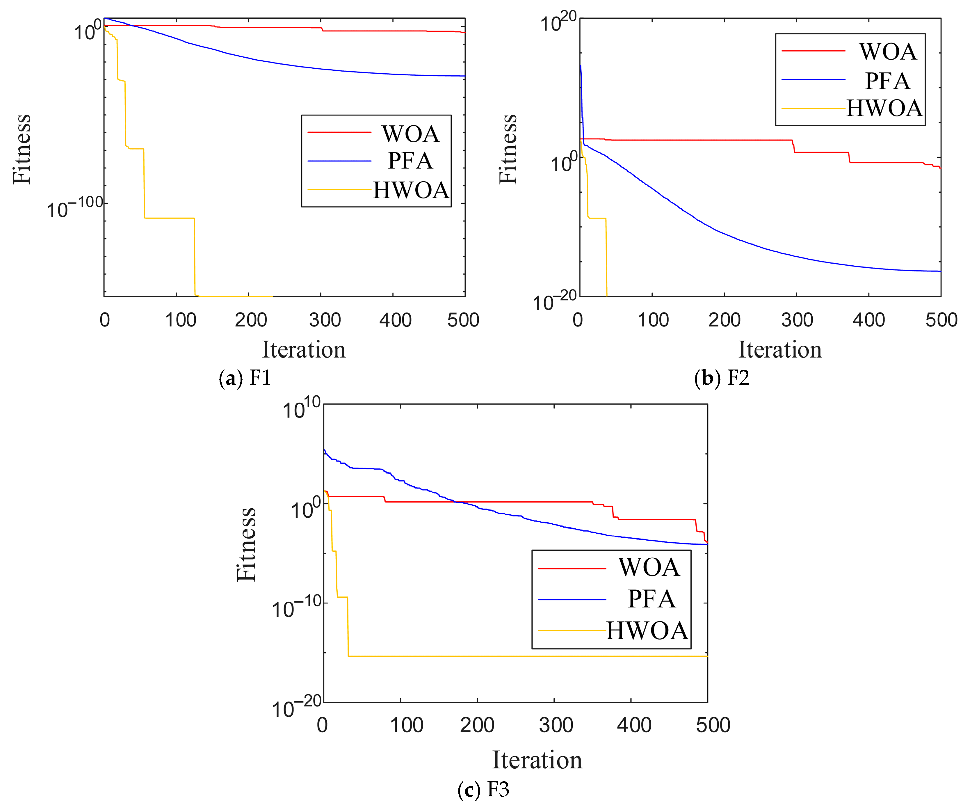
To begin with, the HWOA presented in this study is evaluated against the conventional WOA and the PFA algorithm, frequently utilized in the electrical domain today. A total of 30 optimization search experiments are conducted across three standard test functions, with detailed information about these functions provided in Table 2 [26,27].
The optimization results of the three optimization methods are shown in Figure 4 and Table 3. Compared with the other two algorithms, HWOA exhibits faster search speed and yields better search results in all three standard test functions. Its excellent performance in the multi-peak function indicates that HWOA can better balance the relationship between local and global search.
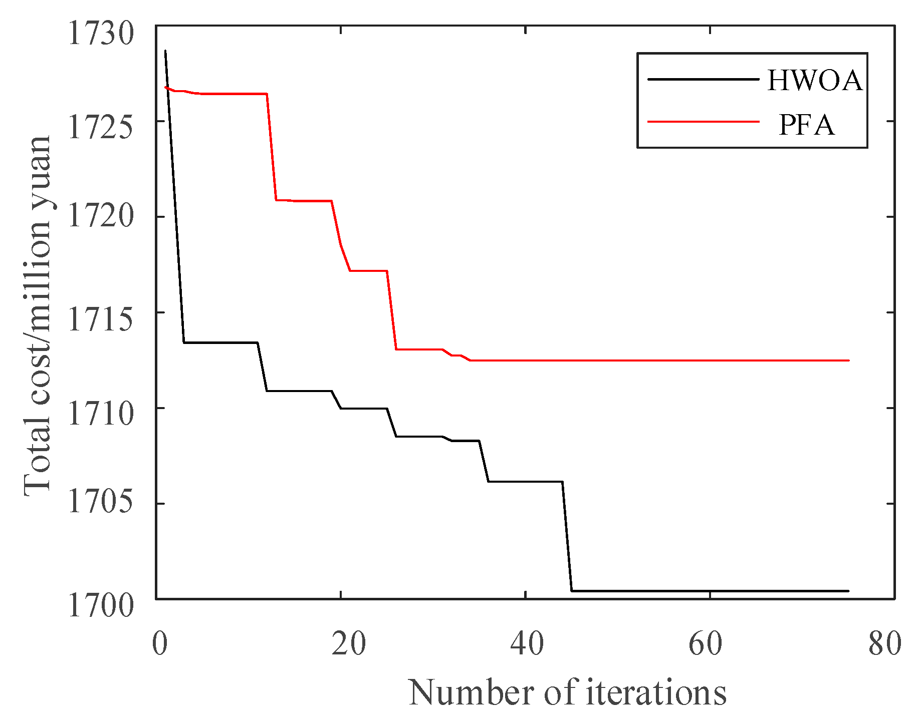
In solving the ADN-BPM optimization problem, PFA and HWOA with better optimization performance are compared. To guarantee an equitable assessment, the highest iteration limit and the population size for each algorithm are established at 75 and 30, accordingly. The outcomes of the optimization are displayed in Table 4, while the simulation convergence characteristic curve is depicted in Figure 5. From the graph, it is evident that local convergence occurs for PFA in the 37th iteration, preventing the attainment of the optimal result. On the other hand, the HWOA algorithm optimization finally converges in 44 iterations, and the algorithm efficiency improves by 18.92% compared to PFA. The total system cost from the optimization is lower for the same number of iterations, showing better optimization capability. The total system cost from the optimization of the HWOA algorithm is reduced by CNY 120,600, and the network loss cost is reduced by CNY 24,200 compared to the PFA. The HWOA algorithm introduced in this study appears to significantly decrease network loss within the system while also minimizing overall system costs, all while considering both the stability and economic efficiency of the system.

4.3. Analysis of Optimization Results

In order to analyze the impact of DR on the total system cost and network loss, two different scenarios are set up to be solved by HWOA to obtain the optimal solution.
Scenario 1: Based on the classical scenario, the DG is sited and sized;
Scenario 2: Based on the classical scenario and considering DR, the DG is sited and sized.
The optimization results for the two distinct approaches are presented in Table 5. When comparing Scenario 1 with Scenario 2, it is evident that, following DR access, there is an 88.77 MWh increase in DG consumption. The effective resolution of uncertainty in new energy generation is achieved through the allocation and scheduling of DG and DR, thereby enhancing system flexibility and efficiency. Network losses are diminished by 6.8 MWh, contributing to an overall improvement in system energy efficiency. Furthermore, the total system cost experiences a reduction of CNY 3.62 million, signifying a noteworthy enhancement in system economics.
To further evaluate the long-term economic viability of the proposed planning strategy, a Net Present Value (NPV) analysis is conducted. The NPV reflects the cumulative discounted benefits of the investment over the project lifetime and is widely used to assess financial feasibility. The NPV is calculated as follows:
N P V = t = 1 T C t C a l l ( 1 + r ) t
where T denotes the DG lifecycle; r denotes the DG discount rate; C t denotes the annual cost saving.
When the NPV is greater than zero, the project is considered profitable. However, whether the investment is worthwhile must be judged by its rate of return. For this purpose, the internal rate of return (IRR) is calculated. It is defined as the discount rate at which the NPV becomes zero.
In Table 5, a discount rate of 8% is adopted. Based on the economic analysis, the IRR is calculated to be about 9%.
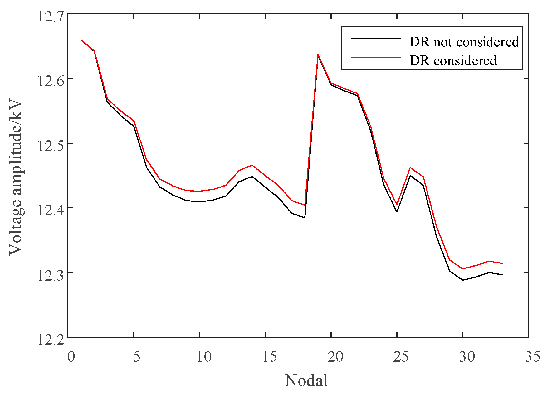
Figure 6 presents the concurrent depiction of voltage distribution across nodes in Scenarios 1 and 2. The illustration reveals a noticeable reduction in voltage amplitude deviation for each node when considering DR. This decline offers benefits in bolstering system power quality and reducing the risk of equipment damage. As a result, it contributes to ensuring the secure and stable operation of the system.
The proposed planning method has been designed to facilitate the integration of renewable energy sources into active distribution networks. In traditional systems, electricity was purchased from upstream thermal power plants at relatively high costs. With the implementation of this approach, renewable energy can be locally generated and consumed through coordinated planning of distributed generation and demand response. As a result, power purchase costs are reduced, and energy self-sufficiency is improved. In addition to economic advantages, the proposed method contributes to sustainability by reducing dependence on fossil fuels and supporting the transition toward cleaner energy systems.
Although the proposed strategy shows good economic performance in simulation, some limitations exist in practical applications. The effectiveness depends on the accuracy of load and generation forecasts. In addition, the response of users cannot always be guaranteed. These factors may reduce the actual benefits when the strategy is applied in real systems.

5. Conclusions

Investigating the two-tier planning challenge within ADNs, this study delves into the incorporation of distributed power sources and DR within the framework of a novel power system. The top layer aims to reduce the yearly overall expenses by carefully determining the positioning and capacity of distributed energy sources. At the same time, the bottom layer tackles the actual system functioning with the goal of decreasing network losses. To address this model, an HWOA is proposed, leveraging co-evolution and adaptive mutation. Utilizing the IEEE33 node arithmetic for testing, the outcomes indicate the following:
  • By incorporating demand response into the ADN planning process, distributed energy consumption can be effectively improved by 88.77 MWh, network loss can be reduced by 6.8 MWh, and the comprehensive cost can be decreased by CNY 3.62 million. This enables the system to operate economically, efficiently, safely, and stably.
  • The HWOA, which considers both global search and local exploration, exhibits excellent optimization performance, with higher accuracy and faster speed in solving the double-layer planning problem for ADNs. Compared to PFA, the algorithm’s efficiency is improved by 18.92%, resulting in a reduction of CNY 120.6 thousand in system assembly derived from optimization and a decrease of CNY 24.2 thousand in network loss cost.
However, in this study, a fixed value is used in setting the Relite of the HWOA, which can be further adaptively optimized, as should many different optimization problems.

Author Contributions

Conceptualization, H.G. and Y.C.; Methodology, H.G.; Software, H.G.; Validation, H.G. and Y.C.; Formal analysis, H.G.; Investigation, H.G.; Re-sources, Y.C.; Data curation, H.G.; Writing—original draft preparation, H.G.; Writing—review and editing, Y.C.; Visualization, H.G.; Supervision, Y.C.; Project administration, Y.C. All authors have read and agreed to the published version of the manuscript.

Funding

This study was supported by the “Key Laboratory of Smart Grid of Ministry of Education for Tianjin University”.

Institutional Review Board Statement

Not applicable.

Informed Consent Statement

Not applicable.

Data Availability Statement

The original contributions presented in this study are included in the article. Further inquiries can be directed to the corresponding author.

Acknowledgments

The author is deeply grateful to his parents for their support, to Yanbo Che for his patient guidance, to lab mates Xiao Guo, Yaling Sun, and Nan Jiang for their valuable help, and to roommates Yunfei Wu, Juewei Lin, and Hao Wang for their encouragement.

Conflicts of Interest

The authors declare no conflicts of interest.

References

  1. Song, M.; Zheng, H.; Shen, Z. Whether the Carbon Emissions Trading System Improves Energy Efficiency—Empirical Testing Based on China’s Provincial Panel Data. Energy 2023, 275, 127465. [Google Scholar] [CrossRef]
  2. Li, Y.; Feng, B.; Wang, B.; Sun, S. Joint Planning of Distributed Generations and Energy Storage in Active Distribution Networks: A Bi-Level Programming Approach. Energy 2022, 245, 123226. [Google Scholar] [CrossRef]
  3. Razavi, S.-M.; Momeni, H.-R.; Haghifam, M.-R.; Bolouki, S. Multi-Objective Optimization of Distribution Networks via Daily Reconfiguration. IEEE Trans. Power Deliv. 2022, 37, 775–785. [Google Scholar] [CrossRef]
  4. Han, F.; Zhang, X.; Li, M.; Li, F.; Zhao, W. Stability Control for Grid-Connected Inverters Based on Hybrid-Mode of Grid-Following and Grid-Forming. IEEE Trans. Ind. Electron. 2024, 71, 10750–10760. [Google Scholar] [CrossRef]
  5. Huang, Y.; Lin, Z.; Liu, X.; Yang, L.; Dan, Y.; Zhu, Y.; Ding, Y.; Wang, Q. Bi-Level Coordinated Planning of Active Distribution Network Considering Demand Response Resources and Severely Restricted Scenarios. J. Mod. Power Syst. Clean Energy 2021, 9, 1088–1100. [Google Scholar] [CrossRef]
  6. Haghifam, S.; Najafi-Ghalelou, A.; Zare, K.; Shafie-khah, M.; Arefi, A. Stochastic Bi-Level Coordination of Active Distribution Network and Renewable-Based Microgrid Considering Eco-Friendly Compressed Air Energy Storage System and Intelligent Parking Lot. J. Clean. Prod. 2021, 278, 122808. [Google Scholar] [CrossRef]
  7. Huang, Z.; Zhang, Y.; Zheng, F.; Lin, J.; An, X.; Shi, H. Day-Ahead and Real-Time Energy Management for Active Distribution Network Based on Coordinated Optimization of Different Stakeholders. Power Syst. Technol. 2021, 45, 2299–2307. [Google Scholar]
  8. Zhang, Z.; Lei, D.; Li, J.; Xu, Y.; Luo, J. Source-Network-Load-Storage Bi-Level Collaborative Planning Model of Active Distribution Network with SOP Based on Adaptive Epsilon-Dominating Multi-Objective Particle Swarm Optimization Algorithm. Power Syst. Technol. 2022, 46, 2199–2209. [Google Scholar]
  9. Tian, X.; Yang, H.; Ge, Y.; Yuan, T. Site Selection and Capacity Determination of Electric Hydrogen Charging Integrated Station Based on Voronoi Diagram and Particle Swarm Algorithm. Energies 2024, 17, 418. [Google Scholar] [CrossRef]
  10. Yang, M.; Li, J.; Li, J.; Yuan, X.; Xu, J. Reconfiguration Strategy for DC Distribution Network Fault Recovery Based on Hybrid Particle Swarm Optimization. Energies 2021, 14, 7145. [Google Scholar] [CrossRef]
  11. Sun, Q.; Yu, Y.; Li, D.; Hu, X. A Distribution Network Reconstruction Method with DG and EV Based on Improved Gravitation Algorithm. Syst. Sci. Control Eng. 2021, 9, 6–13. [Google Scholar] [CrossRef]
  12. Javadi, M.; Gough, M.; Mansouri, S.; Ahmarinejad, A.; Nematbakhsh, E.; Santos, S.; Catalao, J. A Two-Stage Joint Operation and Planning Model for Sizing and Siting of Electrical Energy Storage Devices Considering Demand Response Programs. Int. J. Electr. Power Energy Syst. 2022, 138, 107912. [Google Scholar] [CrossRef]
  13. Xie, H.; Wang, W.; Wang, W.; Tian, L. Optimal Dispatching Strategy of Active Distribution Network for Promoting Local Consumption of Renewable Energy. Front. Energy Res. 2022, 10, 826141. [Google Scholar] [CrossRef]
  14. Xu, X.; Niu, D.; Peng, L.; Zheng, S.; Qiu, J. Hierarchical Multi-Objective Optimal Planning Model of Active Distribution Network Considering Distributed Generation and Demand-Side Response. Sustain. Energy Technol. Assess. 2022, 53, 102438. [Google Scholar] [CrossRef]
  15. Purlu, M.; Turkay, B.E. Optimal Allocation of Renewable Distributed Generations Using Heuristic Methods to Minimize Annual Energy Losses and Voltage Deviation Index. IEEE Access 2022, 10, 21455–21474. [Google Scholar] [CrossRef]
  16. Xiao, H.; Pei, W.; Deng, W.; Ma, T.; Zhang, S.; Kong, L. Enhancing Risk Control Ability of Distribution Network for Improved Renewable Energy Integration through Flexible DC Interconnection. Appl. Energy 2021, 284, 116387. [Google Scholar] [CrossRef]
  17. Yang, Y.; Bian, R.; Wang, T.; Wei, W.; Jun, Z. Inverse Time Overcurrent Optimization of Distribution Network with DG Based on Improved Gray Wolf Algorithm. Energy Rep. 2022, 8, 237–246. [Google Scholar] [CrossRef]
  18. Hao, J.; Feng, X.; Chen, X.; Jin, X.; Wang, X.; Hao, T.; Hong, F.; Du, X. Optimal Scheduling of Active Distribution Network Considering Symmetric Heat and Power Source-Load Spatial-Temporal Characteristics. Appl. Energy 2024, 373, 123974. [Google Scholar] [CrossRef]
  19. Sperr, F.; Stai, E.; Venkatraman, A.; Krause, T.; Hug, G. Service Restoration in the Medium Voltage Grid Minimizing the SAIDI Contribution After Primary Substation Failures. IEEE Trans. Power Syst. 2024, 39, 66–82. [Google Scholar] [CrossRef]
  20. Mirshekali, H.; Mortensen, L.K.; Shaker, H.R. Reliability-Aware Multi-Objective Approach for Predictive Asset Management: A Danish Distribution Grid Case Study. Appl. Energy 2024, 358, 122556. [Google Scholar] [CrossRef]
  21. Li, Y.; Li, W.; Yuan, Q.; Shi, H.; Han, M. Multi-Strategy Improved Seagull Optimization Algorithm. Int. J. Comput. Intell. Syst. 2023, 16, 154. [Google Scholar] [CrossRef]
  22. Liu, J.; Wang, H.; Li, X.; Chen, K.; Li, C. Robotic Arm Trajectory Optimization Based on Multiverse Algorithm. Math. Biosci. Eng. 2023, 20, 2776–2792. [Google Scholar] [CrossRef]
  23. Chen, B.; Zou, H. Self-Conclusion and Self-Adaptive Variation Particle Swarm Optimization. Comput. Eng. Appl. 2022, 58, 67–75. [Google Scholar]
  24. Wang, H.; Schulz, N. A Revised Branch Current-Based Distribution System State Estimation Algorithm and Meter Placement Impact. IEEE Trans. Power Syst. 2004, 19, 207–213. [Google Scholar] [CrossRef]
  25. Sun, P.; Luo, M.; Sun, Z.; Zhou, K.; Luo, Y.; Liu, T.; Tang, H.; Wang, W. An Improved Approach Based on Cuckoo Search Algorithm for Bi-Level Distributed Wind Generation Planning in Active Distribution Network. Power Syst. Technol. 2016, 40, 2743–2749. [Google Scholar]
  26. Liu, X.; Hayati, H. CCHP Optimization for a Building through Optimal Size of the Prime Mover Considering Energy, Exergy, Economics, and Environmental Aspects. CASE Stud. Therm. Eng. 2022, 39, 102403. [Google Scholar] [CrossRef]
  27. Ghiaskar, A.; Amiri, A.; Mirjalili, S. Polar Fox Optimization Algorithm: A Novel Meta-Heuristic Algorithm. Neural Comput. Appl. 2024, 36, 20983–21022. [Google Scholar] [CrossRef]
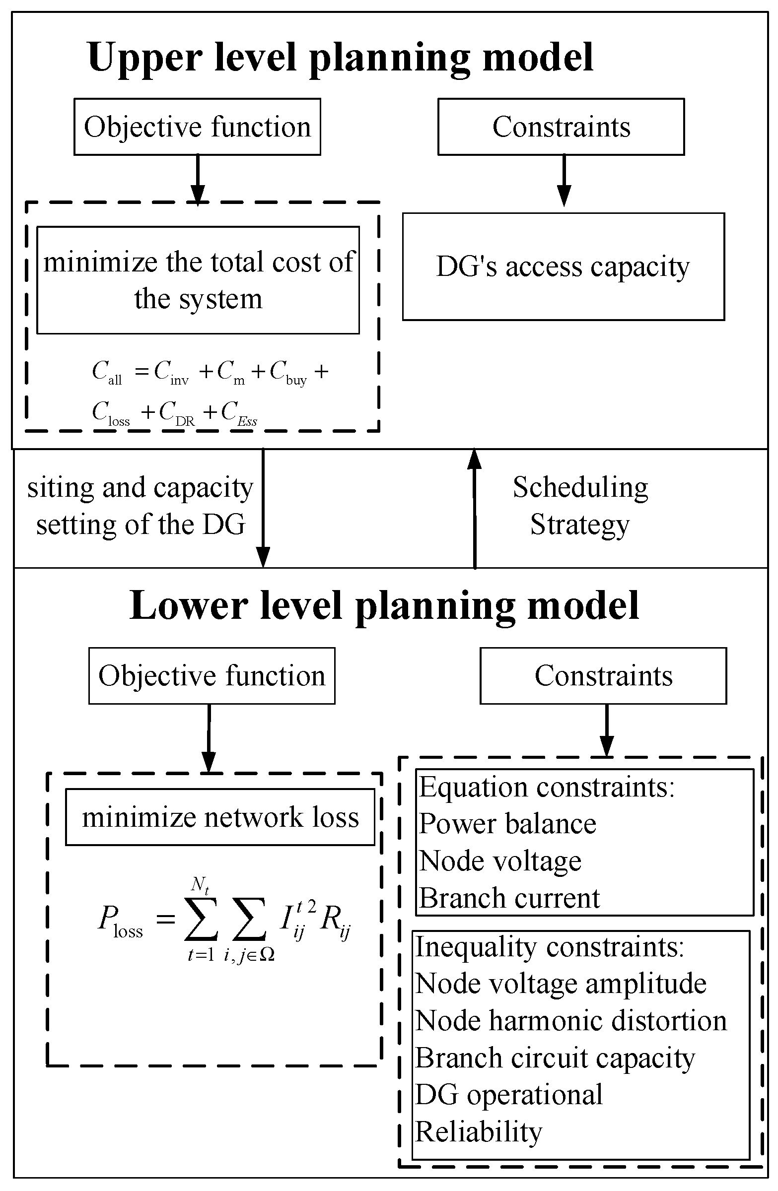
Figure 1. “source-load-network” two-tier planning model.
Sustainability 17 08560 g001
Figure 2. Standard Gaussian distribution and standard Kersey distribution plot.
Sustainability 17 08560 g002
Figure 3. Flowchart of model solving.
Sustainability 17 08560 g003
Figure 4. Convergence curves of WOA, PFA, and HWOA in the standard arithmetic cases.
Sustainability 17 08560 g004
Figure 5. Simulation convergence characteristic curve.
Sustainability 17 08560 g005
Figure 6. Voltage distribution of each node at the same moment in Scenarios 1 and 2.
Sustainability 17 08560 g006
Table 1. System economic indicators.
Project TypeUnitCorrelation Coefficient
DG unit investment costCNY/kVA13
DG discount rate%8
DG lifecycleyears25
DG unit operating costCNY/kWh0.03
Purchase price of electricityCNY/kWh0.4
Grid loss tariffCNY/kWh0.35
DR compensationCNY/kWh1
Table 2. Test Functions for PFA, WOA, and HWOA.
No.Function NameExpressionVariable RangeTheory Extreme Value
F1Sphere f ( x ) = i = 1 n x i 2 [ 100 , 100 ] n 0
F2Rastrigin f ( x ) = i = 1 n x i 2 10 cos 2 π x i + 10 [ 100 , 100 ] n 0
F3Ackley f ( x ) = 20 exp Ackley 0.2 1 n i = 1 n x i 2 exp 1 n i = 1 n cos 2 π x i + 20 + e [ 500 , 500 ] n 0
Table 3. Optimized performance of PFA, WOA, HWOA.
Test FunctionPerformance IndicatorsWOAPFAHWOA
F1Optimum value1.9 × 10−91.7 × 10−340
Average value1.9 × 10−72.0 × 10−330
Standard deviation2.6 × 10−72.6 × 10−330
F2Optimum value8.4 × 10−95.7 × 10−140
Average value3.8 × 10−11.1 × 1000
Standard deviation1.9 × 1002.9 × 1000
F3Optimum value4.1 × 10−64.0 × 10−148.9 × 10⁻¹⁶
Average value4.4 × 10−54.3 × 10−148.9 × 10⁻¹⁶
Standard deviation6.1 × 10−54.3 × 10−150
Table 4. Optimization results of PFA and HWOA.
Optimization ResultsUnitHWOAPFA
DG access point/6, 32, 1427, 12, 25
DG capacitykVA905, 693, 8041048, 837, 803
DG Investment costsk CNY2874.03282.9
DG Running costsk CNY364.3401.1
Power purchase costsk CNY12,716.712,075.7
Net loss costk CNY364.6388.8
DR costk CNY684.6976.3
Total costk CNY17,004.217,124.8
Table 5. Optimization results for Scenarios 1 and 2.
Optimization ResultsOption 1Option 2
DG consumption (MWh)1125.561214.33
DR volume (MWh)068.46
Total system cost (thousand CNY)20,629.817,005.8
Network loss (MWh)110.97104.17
Disclaimer/Publisher’s Note: The statements, opinions and data contained in all publications are solely those of the individual author(s) and contributor(s) and not of MDPI and/or the editor(s). MDPI and/or the editor(s) disclaim responsibility for any injury to people or property resulting from any ideas, methods, instructions or products referred to in the content.