Article

Performance Comparison of LSTM and ESN Models in Time-Series Prediction of Solar Power Generation

Department of System Semiconductor Engineering, Sangmyung University, Cheonan 31066, Republic of Korea
*
Author to whom correspondence should be addressed.
Sustainability 2025, 17(19), 8538; https://doi.org/10.3390/su17198538
Submission received: 14 August 2025 / Revised: 19 September 2025 / Accepted: 21 September 2025 / Published: 23 September 2025

Abstract

Improving the prediction accuracy of solar power generation is a critical challenge in promoting sustainable energy solutions. While machine learning models like long short-term memory (LSTM) have gained attention, they face practical limitations such as their complex structure, long training time, and susceptibility to overfitting. Echo state networks (ESNs) have attracted attention for their small number of trainable parameters and fast training speed, but their sensitivity to hyperparameter settings makes performance improvement difficult. In this study, the key hyperparameters of an ESN (spectral radius, input noise, and leakage rate) were optimized to maximize performance. The ESN achieved a Root Mean Square Error (RMSE) of 0.0069 for power prediction, demonstrating a significant improvement in accuracy over a tuned LSTM model. ESNs are also well-suited for real-time prediction and large-scale data processing, owing to their low computational cost and fast training speed. By providing a more accurate and efficient forecasting tool, this study supports grid operators in managing the intermittency of renewable energy, thereby fostering a more stable and reliable sustainable energy infrastructure.

1. Introduction

Solar power generation is experiencing rapid growth worldwide as it becomes a key component of sustainable energy transition. Global installed solar capacity has grown at an average of more than 20% over the last decade and is expected to reach 5.2 TW by 2030 [1]. This rapid expansion of solar power generation poses new challenges to the reliability and operational efficiency of electricity grids. The most prominent feature of solar power generation is its high variability and intermittency due to weather conditions. Meteorological factors such as solar irradiance, cloud movement, and temperature fluctuations can cause sudden changes in solar power output, and such uncertainty makes reliable grid operation difficult [2]. The accuracy of output forecasts has a direct impact on the reliability of electricity supply and demand, especially in regions where solar power generation capacity accounts for a substantial portion of total generation capacity [3].
Techniques for solar power generation prediction can be broadly categorized into physical models, statistical models, and machine learning-based models. Physical models predict power generation by taking into account solar radiation, atmospheric conditions, and the physical properties of solar cells, but they have limitations in modeling complex weather phenomena and nonlinear relationships [4]. Statistical models such as autoregressive integrated moving average (ARIMA) and seasonal ARIMA (SARIMA) analyze patterns in time-series data to make predictions. However, they have the disadvantage of not fully reflecting the complex nonlinear nature of solar power generation [5]. In recent years, machine learning and deep learning techniques have gained attention in the field of solar power generation prediction. In particular, machine learning models such as artificial neural networks (ANNs), support vector machines (SVMs), and random forests (RFs) outperform traditional statistical models [6,7]. Among deep learning techniques, convolutional neural networks (CNNs), recurrent neural networks (RNNs), and long short-term memory (LSTM) networks have demonstrated excellent performance in solar power generation prediction [8,9]. LSTM networks, a variant of RNNs, were developed to address the problem of long-term dependencies. LSTMs perform well in time-series prediction, owing to their gating mechanism (forget gate, input gate, and output gate), which enables them to selectively retain important information and discard irrelevant data [10]. The performance of LSTM models in the field of solar power generation prediction is highly effective. In various studies, LSTM-based models have achieved 20–30% better prediction accuracy than traditional statistical models, especially for short-term predictions (1–24 h), with Root Mean Square Error (RMSE) in the range of 0.1–0.2 [11,12]. Hybrid models combining CNNs and LSTM models have shown high performance. Some studies have reported high accuracy, with R 2 values of 0.99 or higher [13,14]. However, LSTM models have some important limitations. First, the complex architecture results in long learning times and high computational costs. Second, owing to the large number of parameters, they are prone to overfitting, and this problem is particularly pronounced with limited datasets [15]. Third, the problem of gradient vanishing may not be fully solved and may lead to performance degradation for considerably long sequences [16].
Reservoir computing is a new paradigm for recurrent neural networks, proposed independently by Jaeger and Maass in the early 2000s [17]. The core idea of reservoir computing is to use a fixed random recurrent network (reservoir) to transform the input signal into a high-dimensional space and only train the output layer. This approach considerably simplifies the complex training process of conventional RNNs [18]. Echo state networks (ESNs) are a popular implementation of reservoir computing. An ESN comprises an input layer, a fixed reservoir (hidden layer), and a trainable output layer. The weights of the reservoirs are fixed after initialization, and only the weights of the output layer are learned via least squares [19]. Owing to these structural features, ESNs offer training speeds hundreds of times faster than those of LSTMs and effectively avoid the problem of gradient vanishing [20]. ESNs have performed well on various time-series prediction tasks. In particular, ESNs have achieved higher prediction accuracy and computational efficiency than LSTMs or gated recurrent units (GRUs) in the prediction of chaotic time-series [20]. The potential of ESNs is also recognized in the field of solar power generation prediction. Studies on solar irradiance prediction using multi-reservoir ESNs have achieved performance improvements of more than 10% over traditional methods [21], and some studies have shown that models combining ESNs and kernel extreme learning machines (KELMs) outperform traditional neural networks [22]. However, the biggest challenge for ESNs is the optimization of hyperparameters. Hyperparameters such as the spectral radius, leakage rate, and input noise crucially affect the performance of ESNs, and it is difficult to achieve a performance advantage over LSTMs without proper settings [23].
This study focuses on systematically optimizing the key hyperparameters of an ESN, namely, spectral radius, input noise, and leakage rate, to maximize the performance of solar power generation prediction and to compare and analyze the optimized ESN and LSTM models under the same conditions. The specific procedure of the study is as follows: first, temperature, irradiance, and time (0–23 h cycle) were used as input attributes. These variables were normalized between 0 and 1 to preprocess them into a form suitable for model training. Subsequently, the 720-h dataset was chronologically divided into a training set (the first 80%) and an unseen test set (the final 20%) to build and validate the predictive models. Second, an ESN-based prediction model was designed by fixing the number of hidden units to 50 and setting candidate ranges for three hyperparameters: spectral radius, input noise, and leakage rate. A multidimensional grid search method was then used to systematically test all hyperparameter combinations, and the average RMSE of solar irradiance and power generation predictions was calculated for each combination. The parameter combination with the lowest average RMSE among those explored through grid search was selected as the optimal value. Third, to ensure a fair comparison, the hyperparameters for both the ESN and LSTM models were systematically optimized, and their final predictive performances were compared on the unseen test set using the RMSE metric. Fourth, the prediction results were visualized as a time-series plot to check the consistency of the actual and predicted values, and the hyperparameter optimization results were presented as a three-dimensional scatter plot to intuitively identify the optimal region. Through this multistage evaluation procedure, we experimentally demonstrated that the hyperparameter-optimized ESN model achieves higher prediction accuracy and better computational efficiency than the tuned LSTM model.

2. I-V and P-V Characteristics

The electrical properties of a solar cell are most widely described by a single diode equivalent circuit model [24,25]. The basic equation for this model is as follows:
I = I p h I 0 exp V + I R s n V t h 1 V + I R s R s h
where I is the output current, I ph is the photocurrent, I 0 is the saturation current, V is the voltage of the solar cell, R s is the series resistance, n is the ideality factor, and V t h is the thermal voltage V t h = k T q . Moreover, k is the Boltzmann constant, T is the temperature, q is the electron charge, and R s h is the parallel resistance [26]. The photocurrent in a solar cell varies with temperature and solar irradiance, which is represented by the following equation:
I ph = I sc + K i T T ref G G ref
where I s c is the short-circuit current, K i is the temperature coefficient of the current, T r e f is the reference temperature, G is the solar irradiance, and G r e f is the reference irradiance. This model is important for accurately predicting how the performance of a solar cell changes with changes in temperature and irradiance. The power-voltage P-V curve of a solar cell, which is the product of voltage and current, can be represented as P = V × I . This relationship is important for understanding the maximum power point (MPP), where solar cells operate at optimal efficiency. At the MPP, the conditions in d P d V = 0 are met, which are key to optimizing the efficiency of a PV system. The simulated I-V and P-V curves based on the temperature and irradiance data for one month are presented in Figure 1a,b.
Figure 1 presents the simulated I-V and P-V curves for the two seasonal datasets used in this study, generated using Equations (1) and (2). Figure 1a,b show the characteristics for the spring period, while (c) and (d) represent the more volatile winter period. These curves are based on time-varying temperature and irradiance data over a 30-day period. The color variations in the curves represent different times of the day, with each line corresponding to a specific time point. Using the given temperature and irradiance data, we calculated I ph to find the current in the solar cell. The P–V curve is a plot of the current I and voltage V values at each time of day. These values can be used to calculate the power of the solar cell P at each time of the day. For this study, we used the following settings: I 0 = 1 × 10 10   A , R s = 0.01   Ω , n = 1.3, V t h = 0.0259   V (based on a temperature of 25   ° C ), R s h = 250 Ω ,   I s c = 5.7   A , K i = 0.003   A / ° C , T r e f = 25   ° C , solar irradiance G at each (based on the given data), G r e f = 1000   W / m 2 , respectively [27].

3. Principle of LSTM Networks and Echo State Networks

3.1. Machine Learning in Time-Series Prediction

For solar power forecasting, a variety of machine learning models have been proposed, ranging from traditional methods like Support Vector Regression (SVR) to state-of-the-art architectures like Transformers. However, for time-series data, RNNs and their variants are often favored due to their inherent ability to capture temporal dependencies, a task where static models like SVR can be limited [28]. While Transformers have shown excellent performance on large-scale sequence tasks, they are known to be data-hungry and computationally intensive, often leading to overfitting and poor performance on smaller datasets [29]. Given the limited 30-day dataset used in this study, we concluded that a Transformer-based approach would not be suitable. Therefore, this study focuses on a direct comparison within the RNN family, specifically between the widely used LSTM network and the ESN, a promising alternative known for its computational efficiency and suitability for modeling dynamic systems. The goal is to evaluate the practical advantages of a systematically optimized ESN as a more efficient yet powerful solution for real-world solar power forecasting tasks.

3.2. LSTM Networks

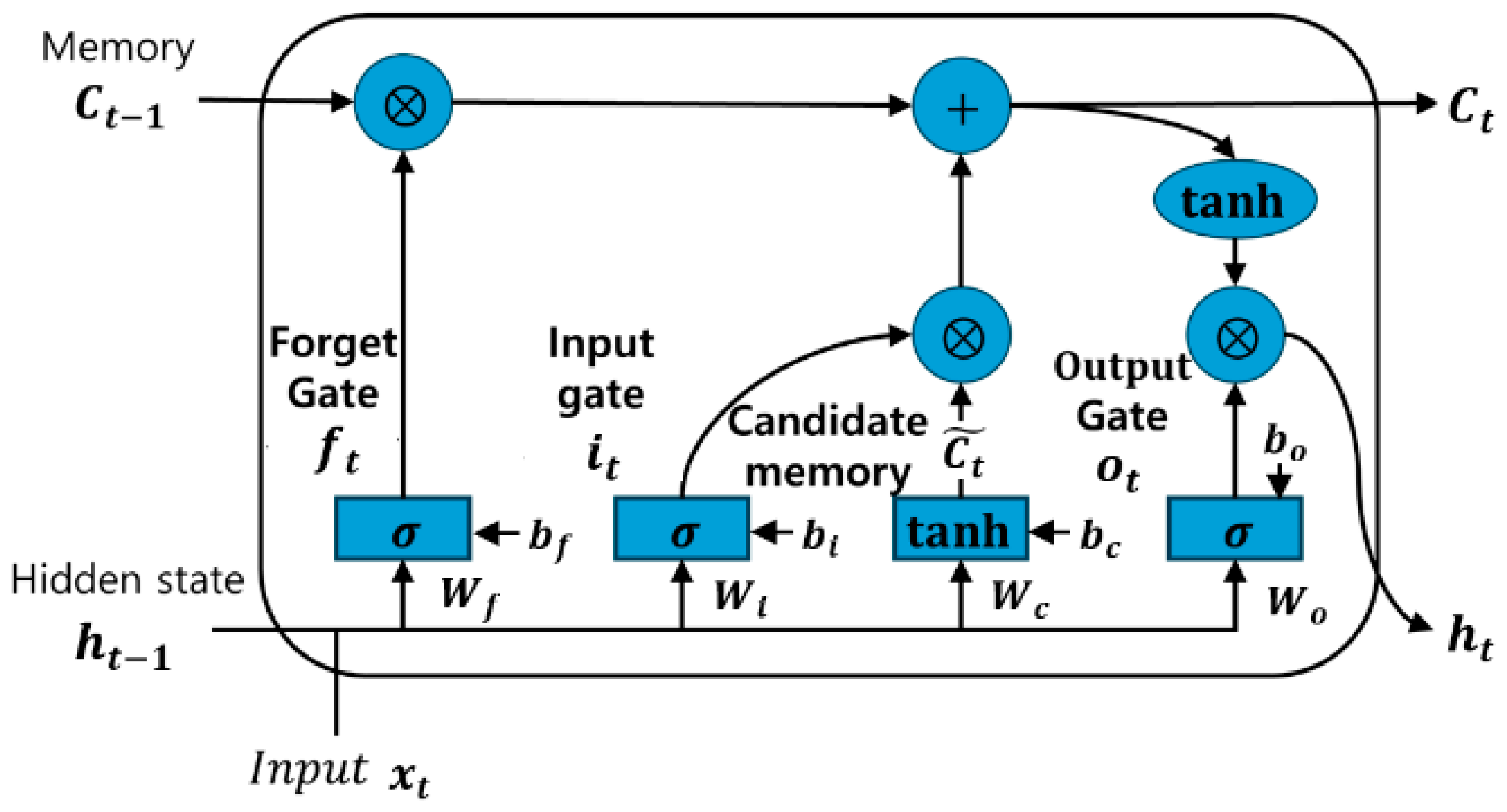
LSTMs are an extension of recurrent neural networks, which were developed to solve the long-term dependence problem of traditional RNNs [30]. LSTMs are designed to effectively learn dependencies in time-series data over long periods of time through an internal gating mechanism [30]. An LSTM cell comprises three core gates: the forget gate, input gate, and output gate [31]. These gates control the flow of information by retaining important information and removing unnecessary information. The forget gate determines the information that should be removed from the state of the cell at a previous point in time. The formula is as follows [31].
f t = σ W f h t 1 , x t + b f
where f t is the output of the forget gate at the current point in time, σ is the sigmoidal activation function, W f is the forget gate weight matrix, h t 1 , x t is the association of the previous hidden state with the current input, and b f is the bias vector [31]. The input gate determines the part of the new information that should be stored in the cell state [30]. The expression is as follows [30]
i t = σ W i h t 1 , x t + b i
The candidate cell state generates new information to be added to the cell. The expression is as follows [30].
C t ~ = tanh W C h t 1 , x t + b C
The cell state is updated by combining the outputs of the forgetting gate and the input gate [31]. The expression is as follows.
C t = f t C t 1 + i t C t ~
The output gate controls the information to be passed from the cell state to the hidden state at the current time [30].
o t = σ W o h t 1 , x t + b o
h t = o t tanh C t
Figure 2 shows the internal structure of an LSTM cell.

3.3. Echo State Networks

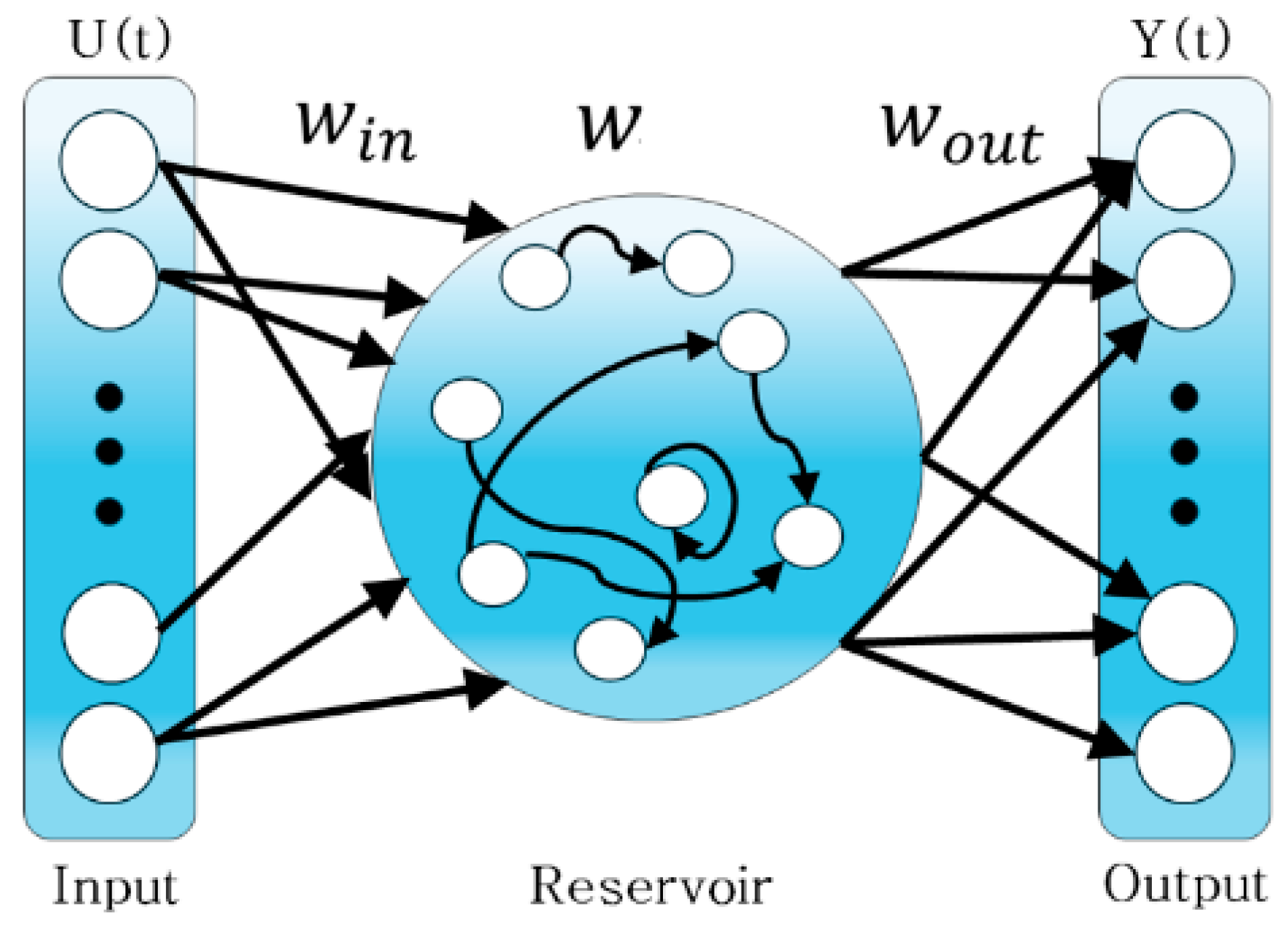
Reservoir computing is a computational model based on dynamic simulations, which provides a structure for efficient processing of complex temporal patterns via nonlinear mapping of input data into a high-dimensional space [32,33]. As a typical implementation, ESNs, a type of RNNs, are effectively applied to problems with temporal dependencies, such as time-series data [17,34]. The core structure of ESNs consists of an input layer, a fixed reservoir, and an output layer [17]. The main feature is that the hidden layer comprises a randomly initialized recurrent network with fixed weights during the learning process [32,33]. This reservoir dynamically projects the input signal into a high-dimensional state space to represent its complex feature and is responsible for the nonlinearity of the entire network [17]. Furthermore, the learning process is simple and fast by learning only the weights of the output layer. This also alleviates the problem of overfitting [17]. Owing to the aforementioned structure, ESNs can effectively avoid the problem of gradient vanishing or runaway, which is common in traditional RNNs, and can achieve good performance with low computation [17,33]. In particular, it utilizes the dynamic nature of reservoirs to represent input sequences in high-dimensional space, making it well suited for prediction and classification problems with complex temporal patterns [32,33].
Figure 3 shows the structure of an echo state network. An ESN consists of an input layer, a fixed reservoir, and an output layer. The dynamics of an ESN are defined by the update of its internal state and the computation of its output. Let u t R K be the input vector, x t R N be the internal reservoir state vector, and y t R L be the output vector at time step t . Then, the dynamics of the ESN can be expressed by the following formula [17,32]:
x t = 1 α x t 1 + α tanh W in u t + W x t 1 + b
where W in R N × K is the input weight matrix, W R N × N is the internal weight matrix of the reservoir, α is the leaking rate, and b is the bias vector [17,35]. The expression for calculating the output is as follows. u t is substituted by a parameter u ~ t created by adding noise to the input vector [35,36].
u ~ t = u t + ε t ,   ε t N 0 , σ 2
where ε t is an additive white Gaussian noise (AWGN) with a mean of 0 and a standard deviation (noise amplitude) of σ [35,36].
y t = W o u t u ~ t x t
where W o u t is the output weight matrix [17]. The states of the reservoir form a high-dimensional nonlinear dynamical system, which can effectively represent the temporal pattern of the input sequence [17,33]. In addition, a key feature of the ESN is that the internal reservoir weights W and W i n are fixed after initialization [17]. Therefore, only the weights of the output layer W o u t are learned; to achieve this, the reservoir states x t from all training time steps are collected into a state matrix X, and the corresponding target outputs are collected into matrix Y target . The output weights are then computed via the least square method as follows [17]:
W out = Y target X
where Y target is the set of target outputs and X is the Moore–Penrose pseudoinverse of X . For ESNs to operate reliably, they must satisfy the echo state property [37]. This is a property that allows (i) the dependency on the initial state to disappear over time and (ii) the state of the reservoir to be determined by the input. The following condition is generally used to satisfy this property.
p W < 1
where p W is the spectral radius of the reservoir weight matrix W , which should be set to less than 1 to ensure that the dynamic system of the reservoir converges stably [17,37].

3.4. Performance Evaluation Metrics

To quantitatively evaluate and compare the prediction performance of the proposed LSTM and ESN models, RMSE was selected as the primary evaluation metric. RMSE is a standard metric for regression tasks that measures the average magnitude of the errors between predicted and actual values. It is particularly sensitive to large errors, making it a suitable indicator for prediction accuracy in volatile time-series data such as solar power generation, The RMSE is calculated as follows:
R M S E = 1 n i = 1 n y i y i ^ 2
where n is the total number of data points, y i is the actual value, and y i ^ is the predicted value. A lower RMSE value indicates a better fit of the model to the data, signifying higher prediction accuracy. This metric will be used to compare the final performance of both models in Section 4 [38].

3.5. Experimental Design and Validation

A consistent experimental framework was established to ensure a fair comparison between the ESN and LSTM models. All input and target variables were first normalized to a [0, 1] range using a MinMaxScaler. The 720-h time-series sequence data was then chronologically split into an 80% training set (the first 576 h) and a 20% unseen test set (the final 144 h). While the data splitting and evaluation procedures were identical, distinct hyperparameter optimization strategies were employed for each model in the training set. For the ESN, while advanced methods like Bayesian Optimization are applicable for hyperparameter tuning in reservoir computing [39], this study employed a systematic Grid Search to exhaustively test combinations of its key hyperparameters (spectral radius, input noise, and leaking rate). For the LSTM, efficient Bayesian Optimization [40], implemented with the Optuna framework [41], was employed for 100 trials to search for the optimal combination of hidden units, number of layers, and learning rate.

4. Simulation Results and Performance Comparison

4.1. Dataset and Experimental Setup

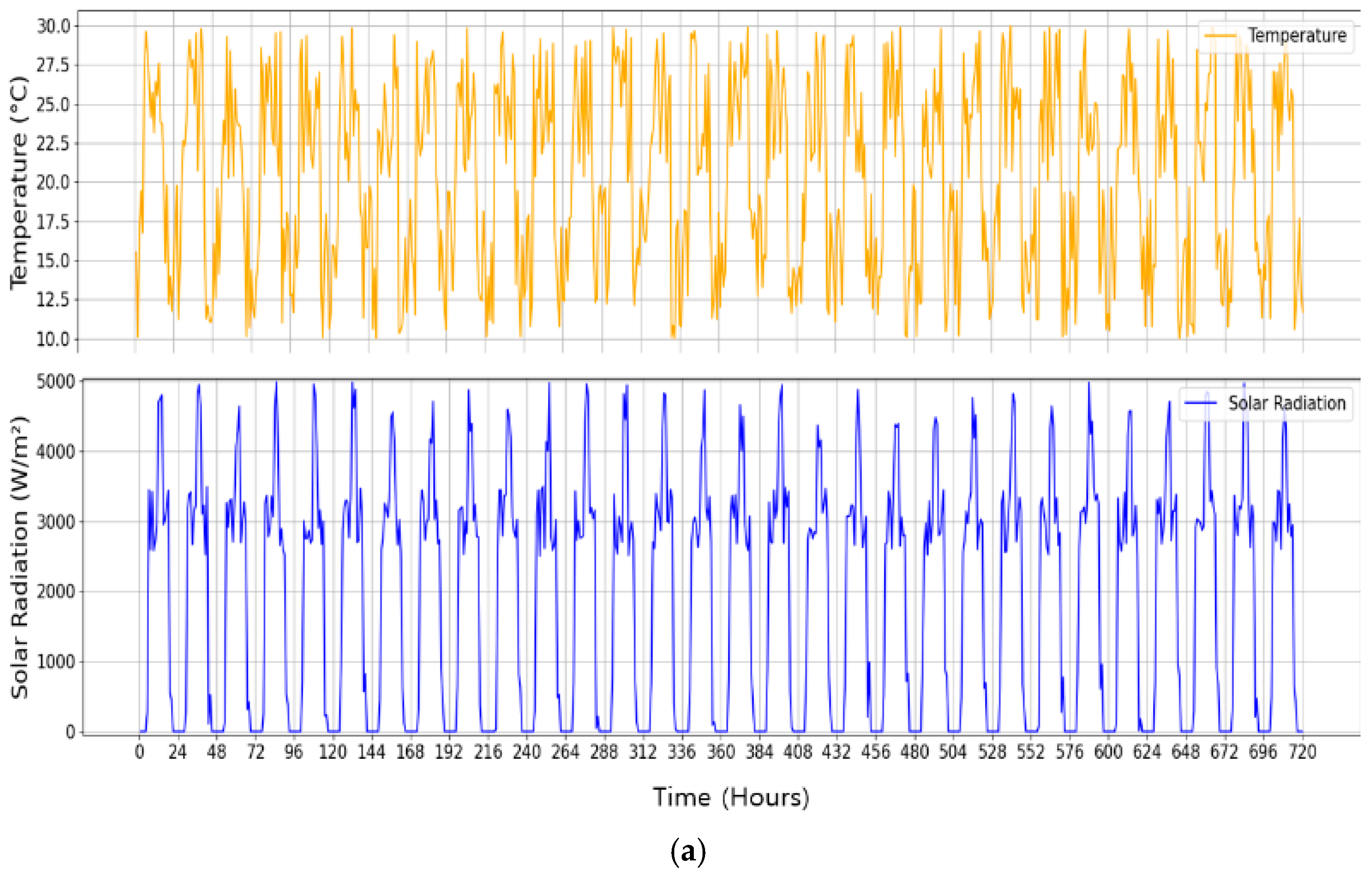
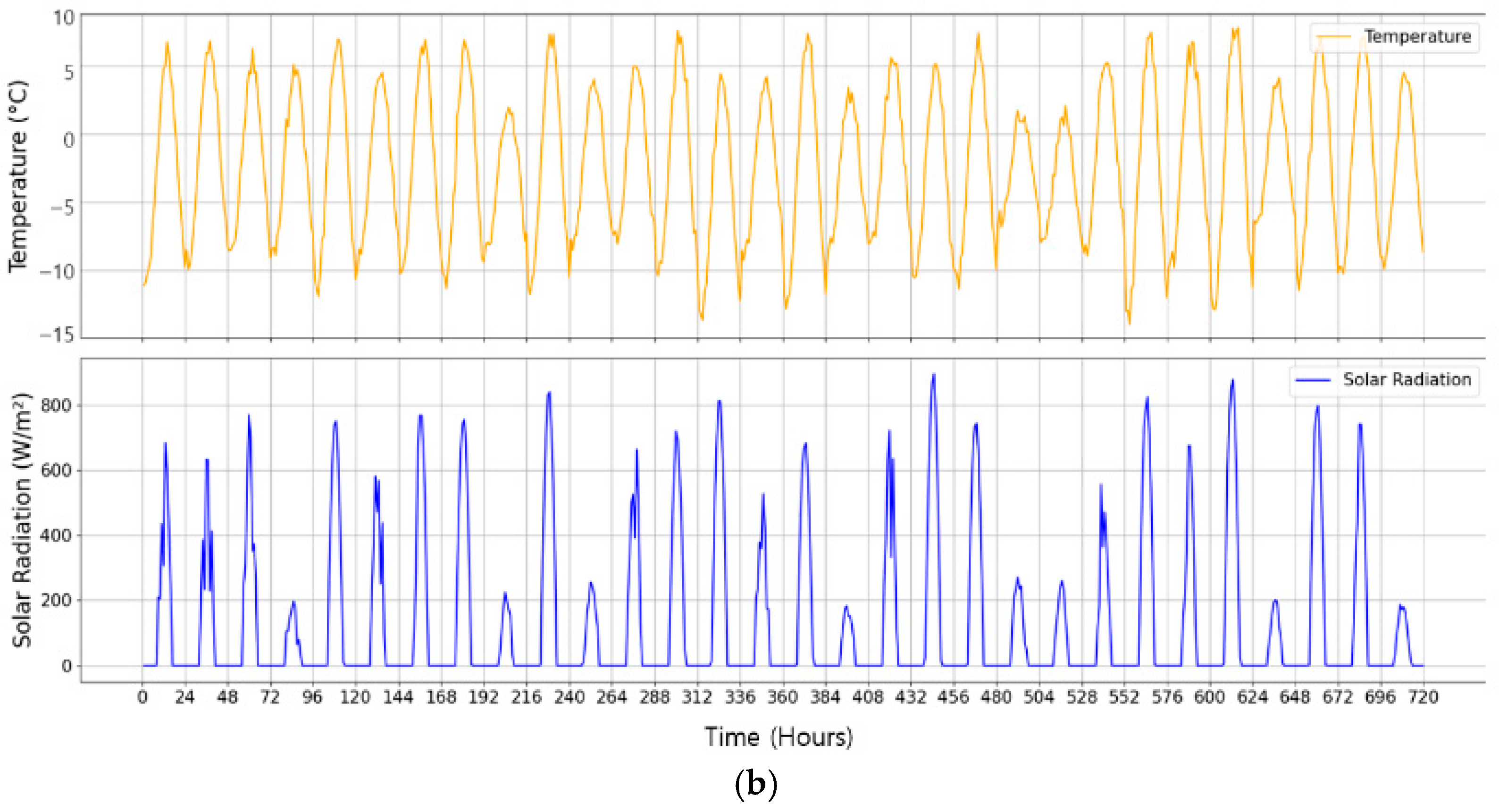
To evaluate without loss of generality of the models across different climatic conditions, this study utilizes two distinct 30-day hourly datasets sourced from South Korea, representing contrasting seasonal patterns. Figure 4 visualizes the time-series data for both datasets used in this study. Figure 4a shows Dataset A, which is characterized by stable, periodic daily patterns with higher temperatures, typical of spring conditions. In contrast, Figure 4b displays Dataset B, which exhibits more variable solar irradiance and significantly lower temperatures, representing more challenging winter conditions. A key aspect of our methodology is that the ‘True Power Output’ for both datasets was generated using the physical model detailed in Section 2 (Equations (1) and (2)). This physics-based ground truth was then used to train and evaluate the models based on an 80% training and 20% test split.

4.2. LSTM Simulation

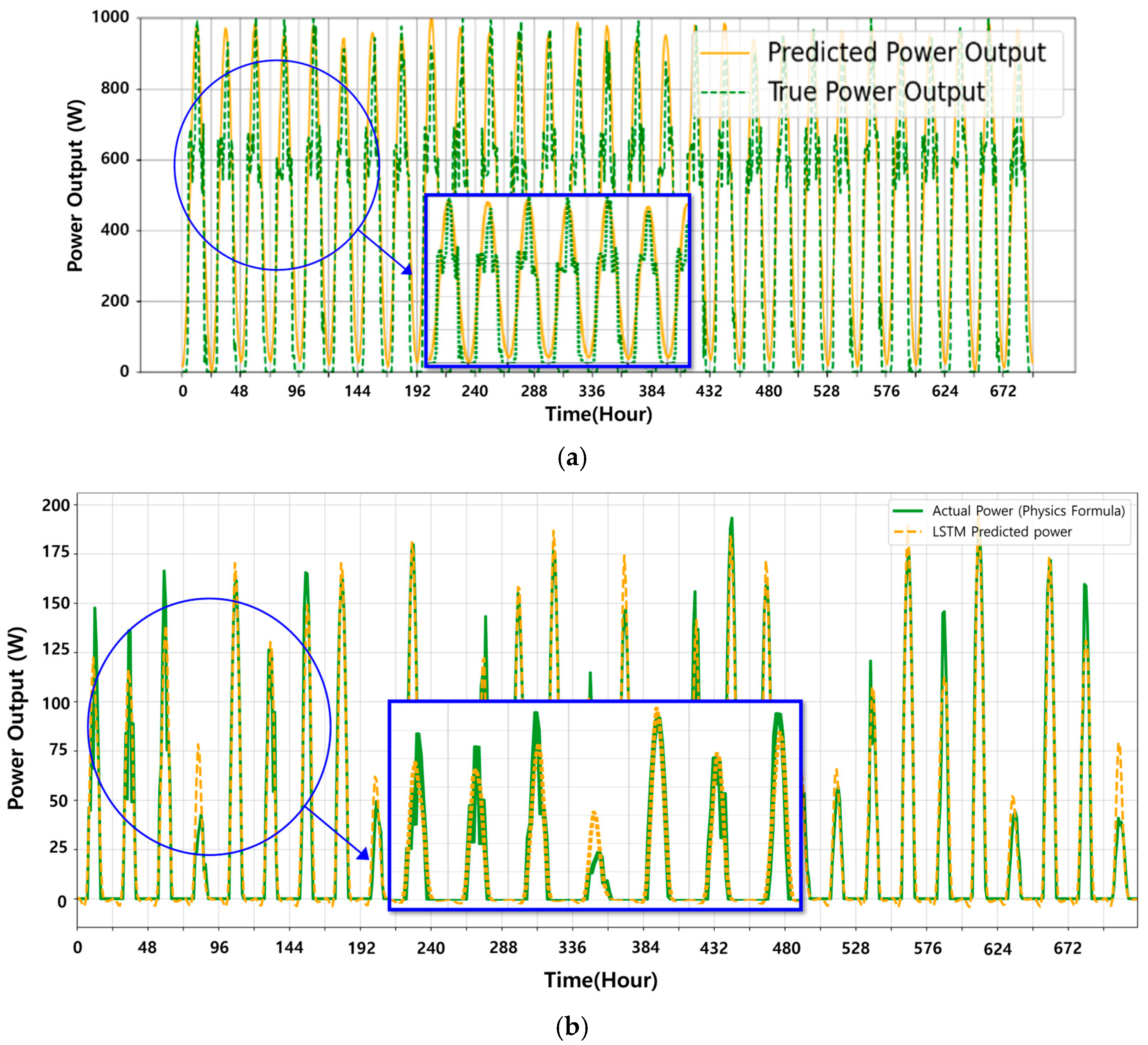
Figure 5 shows the solar power predicted by an LSTM for 30 days. The simulation results were analyzed based on the RMSE. The LSTM’s RMSE was found to be between 0.007 and 0.1 on average.
The LSTM model used in this study is internally processed by the PyTorch LSTM, where the equations from Equation (3) to Equation (8) are implemented to learn the time-series data. To ensure a fair comparison with the optimized ESN, the LSTM model was also subjected to a rigorous hyperparameter optimization process. A Bayesian optimization approach [40], implemented with the Optuna framework [41], was employed for 100 trials to efficiently search for the optimal configuration. The search space included key hyperparameters such as the hidden state size (16 to 128), the number of layers (from 1 to 3), and the learning rate (from 1 × 10 4 to 1 × 10 2 ). For the stable spring data, the optimal configuration was found to be a hidden size of 32, 3 layers, and a learning rate of 0.009, which achieved an RMSE of 0.072. For the more volatile winter data, which presents a more challenging forecasting task, the best-performing model was configured with a hidden size of 128, 3 layers, and a learning rate of 0.008, resulting in an RMSE of 0.094.

4.3. ESN Simulation

ESNs are neural network models that are suitable for modeling dynamic systems and can effectively model changes over time in solar energy generation systems. These models use input layers (temperature and irradiance) and reservoirs (dynamic conversion) to finally generate output layers (predicted power generation). To optimize the performance of these models, we optimized hyperparameters such as the spectral radius, input noise, and leaking rate using a grid search.
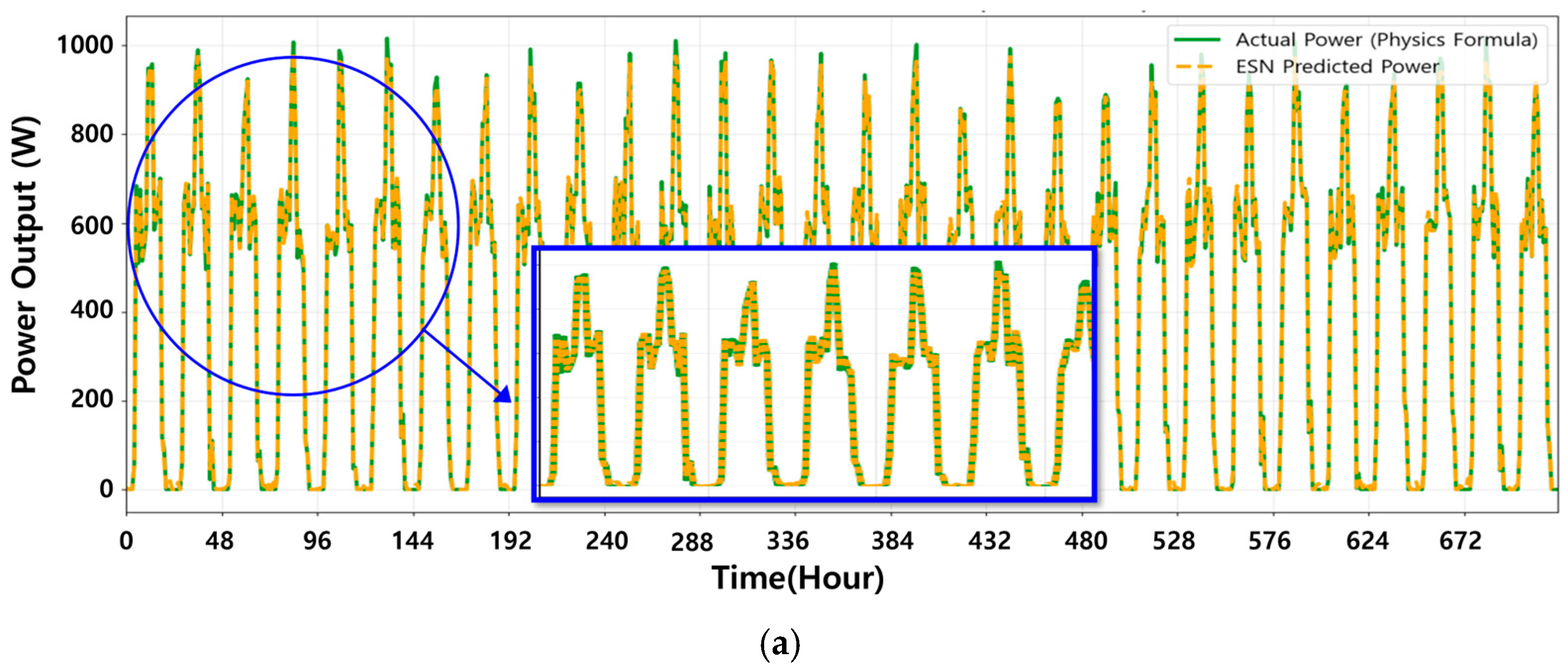
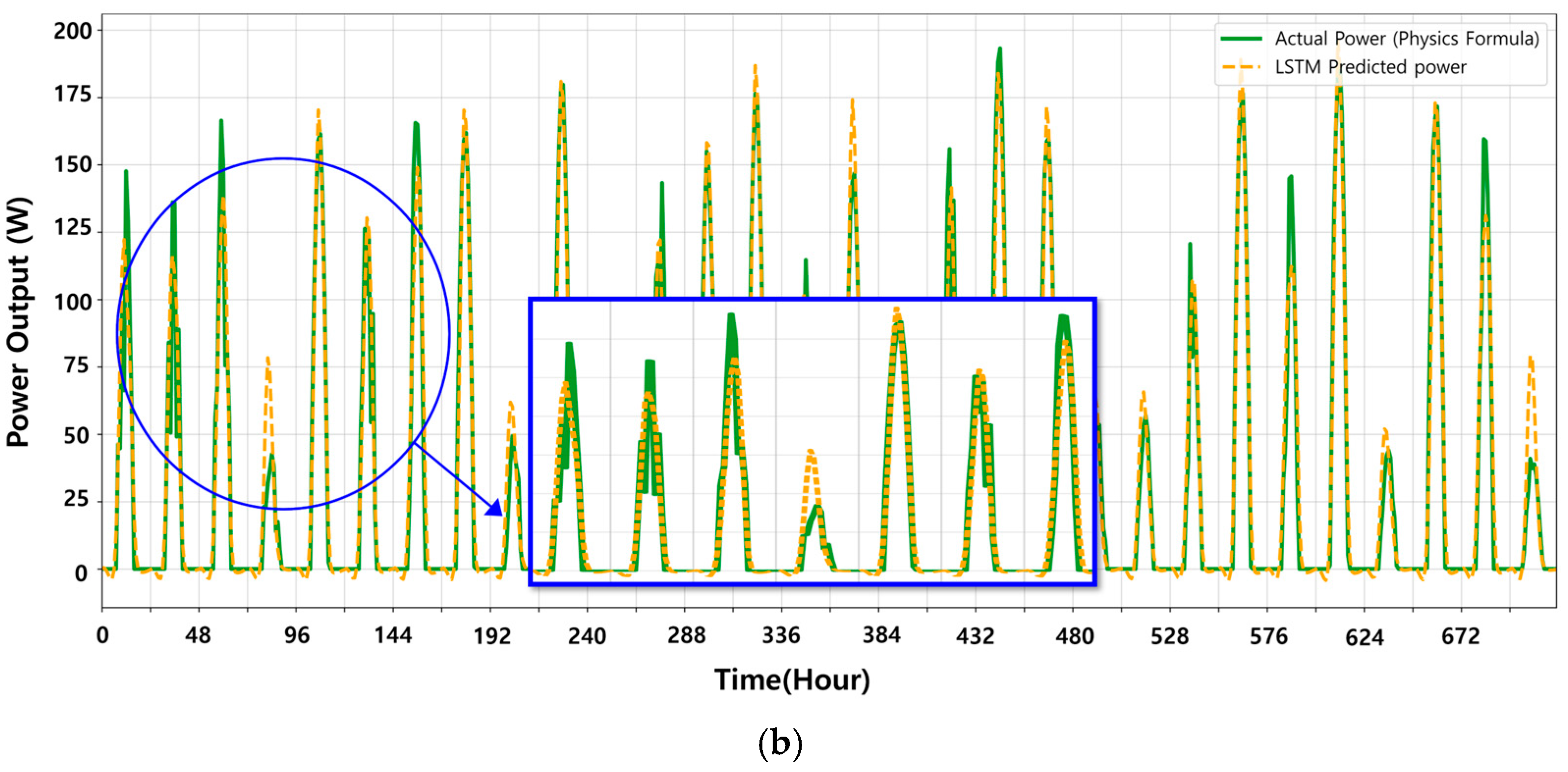
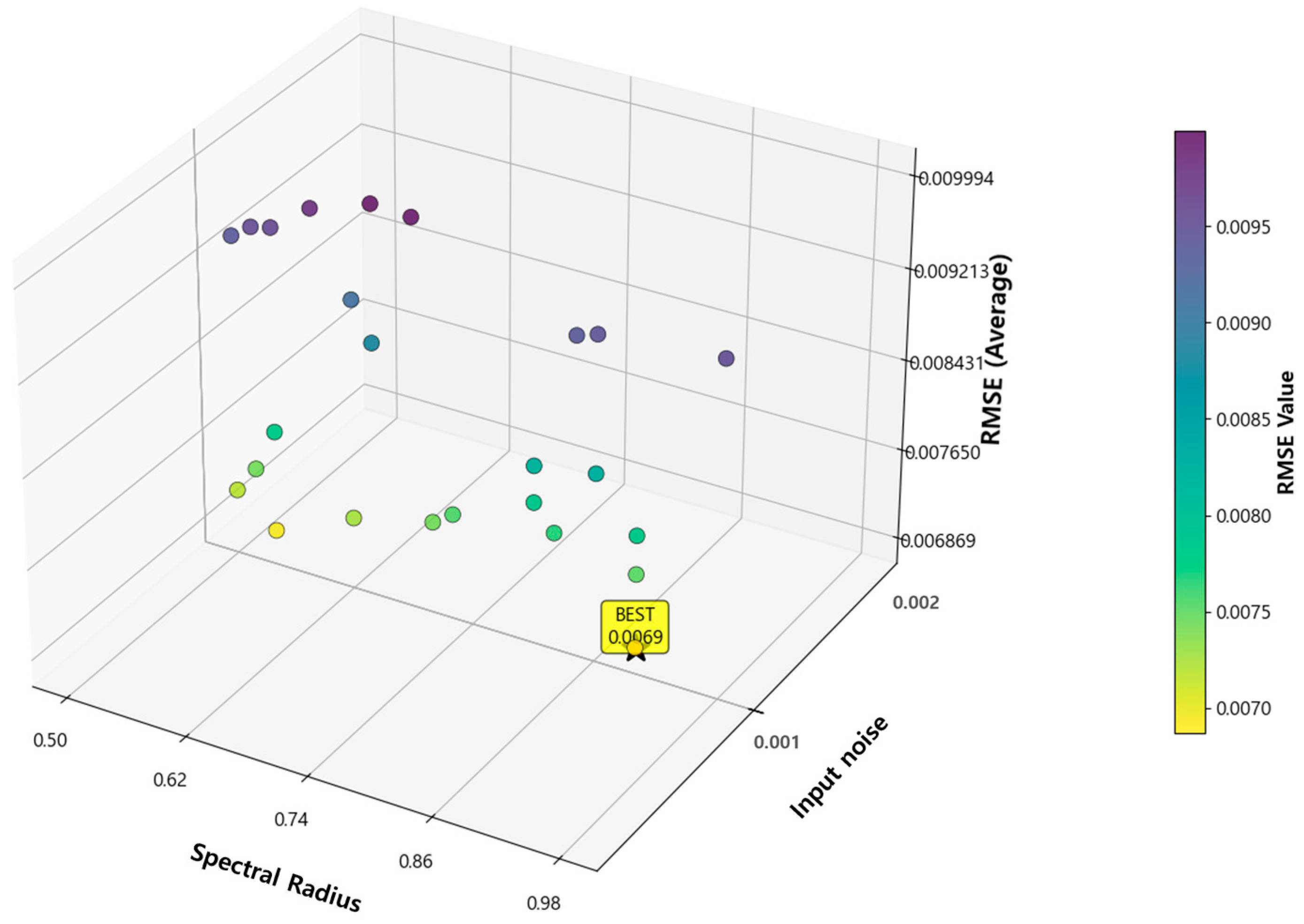
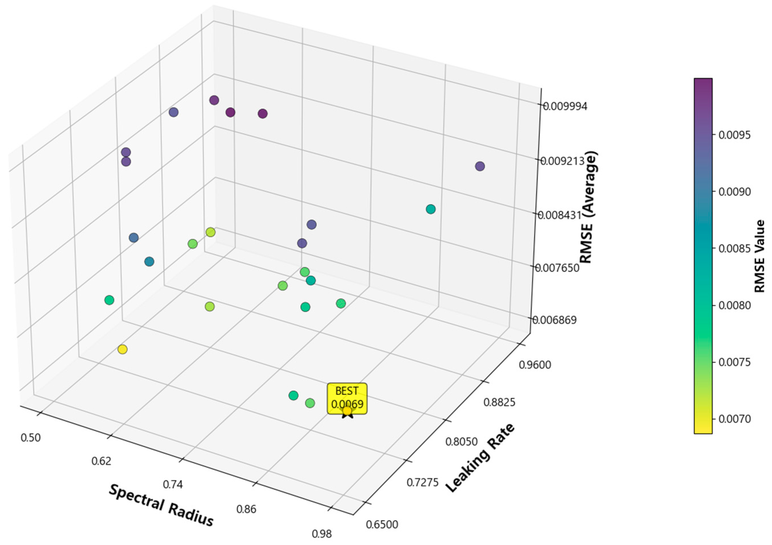
The performance was evaluated by comparing the predicted results with the actual values. The visualization analyzed the relationship between the hyperparameters and RMSE using graphs and 3D graphs comparing the actual data with the predicted values and identified the optimal hyperparameter combinations. The actual power generation was calculated according to the physical formula through Equations (1) and (2). The performance metrics for an ESN model based on optimized hyperparameters are as follows. For the stable spring data, shown in Figure 6a, the optimal hyperparameter combination was a spectral radius of 0.900, the input noise of 0.001, and a leaking rate of 0.750. This configuration achieved a power generation prediction RMSE of 0.0069. For the more challenging winter data, presented in Figure 6b, the best-performing model was configured with a spectral radius of 0.870, input noise of 0.001, and a leaking rate of 0.810. This resulted in an RMSE of 0.0097. Figure 7 and Figure 8 visualize the grid search process, illustrating how the RMSE varies across different hyperparameter combinations.
In RC coupling parameter search, the goal is to select suitable and potentially optimal coupling parameters, a leaking rate α and noise amplitude σ , such that the RC dynamics remain bounded while generating rich patterns in the internal states. Empirical studies suggest that choosing α and σ so that the system lies at the edge of chaos generally yields the best results, which is supported by a necessary condition imposed on the largest singular value of the effective stability matrix.

4.4. Comparison with Previous Studies

To contextualize the performance of our proposed model, we compared our results with those reported in the recent literature for similar solar forecasting tasks, as summarized in Table 1. Conventional LSTM models have reported normalized RMSE values in the range of 0.082 to 0.090 [42,43]. Even advanced hybrid models, such as the CNN-LSTM architecture proposed by Khan et al. [44], achieved an RMSE of approximately 0.075. Our own LSTM model achieved a best-case RMSE of 0.072 and 0.094, demonstrating competitive performance against these benchmarks. However, the systematically optimized ESN in our study achieved a significantly lower RMSE of 0.0069 and 0.0097, outperforming not only the models in the recent literature but also our own rigorously tuned LSTM. This suggests that a systematically optimized ESN can be a more resource-efficient yet equally, if not more, powerful alternative for this forecasting task.

5. Conclusions

This study conducted a comparative analysis of a hyperparameter-optimized ESN against a tuned LSTM model for solar power forecasting. The findings indicated that, under the specific conditions of this study, a systematically optimized ESN serves as a highly efficient and powerful alternative. The ESN achieved a lower RMSE of 0.0069, not only outperforming the tuned LSTM but also demonstrating highly competitive performance against more complex deep learning architectures reported in the recent literature. Furthermore, the ESN’s significantly faster training speed underscores its practical advantage for real-world applications, requiring frequent model retraining with new data. For grid operators, this translates to significant practical benefits: rapid retraining allows for more responsive forecasting, which can lead to better supply-demand balancing, reduced reliance on expensive fossil-fuel reserves, and enhanced overall grid stability. A key factor in this improvement was the tuning of input noise, which acts as a form of regularization, preventing the model from overfitting and thereby enhancing its generalization capability. This highlights that meticulous hyperparameter optimization, rather than increased model complexity, can be a key driver for achieving state-of-the-art forecasting accuracy. However, these findings must be interpreted within the context of the study’s limitations. The models were evaluated on a limited 30-day dataset from a single location, which may not capture diverse seasonal patterns or more volatile climatic conditions. Consequently, the generalizability of these results requires further validation on larger, multi-site datasets to be fully established. In conclusion, this research highlights the significant potential of optimized ESNs as a computationally efficient and robust tool for solar power forecasting. While further validation is necessary, our study suggests that ESN-based approaches are a promising direction for developing practical alternatives to more complex deep learning models, contributing to more efficient and sustainable energy management.

Author Contributions

Conceptualization, Y.J. and J.L.; methodology, Y.J., D.K., Y.N. and J.C.; software, Y.J., D.K., Y.N. and J.C.; validation, Y.J., D.K. and J.L.; writing—original draft preparation, Y.J.; writing—review and editing, Y.J., D.K., Y.N., J.C. and J.L.; visualization, Y.J.; supervision, J.L.; project administration, J.L.; funding acquisition, J.L. All authors have read and agreed to the published version of the manuscript.

Funding

This work is funded by a 2025 research Grant from Sangmyung University.

Institutional Review Board Statement

Not applicable.

Informed Consent Statement

Not applicable.

Data Availability Statement

The data present in this study are available upon request from the corresponding author.

Conflicts of Interest

The authors declare no conflicts of interest.

References

  1. International Energy Agency. Solar PV Global Supply Chains; International Energy Agency: Paris, France, 2022. [Google Scholar]
  2. Wang, H.; Li, X.; Zhang, Y.; Chen, Z. A Review of Deep Learning for Renewable Energy Forecasting. Energy Convers. Manag. 2019, 198, 111–121. [Google Scholar] [CrossRef]
  3. Benti, N.E.; Chaka, M.D.; Semie, A.G. Forecasting Renewable Energy Generation with Machine Learning and Deep Learning: Current Advances and Future Prospects. Sustainability 2023, 15, 7087. [Google Scholar] [CrossRef]
  4. Liu, X.; Zhao, Q.; Sun, Y. Investigating the Power of LSTM-Based Models in Solar Energy Forecasting. Processes 2023, 11, 425–438. [Google Scholar]
  5. Patel, R.; Gupta, S. Solar Radiation Prediction: A Multi-Model Machine Learning and Deep Learning Approach. AIP Adv. 2025, 15, 125101. [Google Scholar] [CrossRef]
  6. Chen, L.; Wang, M.; Huang, G. Comparison of AI-Based Forecasting Model ANN, CNN, and ESN for Forecasting Solar Power. Int. J. Innov. Sci. Adv. Eng. 2024, 10, 45–57. [Google Scholar]
  7. Singh, A.; Kumar, P.; Sharma, T. Hybrid Deep Learning CNN-LSTM Model for Forecasting Direct Normal Irradiance. Nat. Sci. Rep. 2025, 15, 9876. [Google Scholar]
  8. Zhao, L.; Chen, H. Solar Power Prediction Using Dual Stream CNN-LSTM Architecture. Sensors 2023, 23, 3287. [Google Scholar] [CrossRef]
  9. Martínez, J.; Fernández, I. Deep Learning Models for PV Power Forecasting: Review. Energies 2024, 17, 1123. [Google Scholar] [CrossRef]
  10. Santos, R.; Almeida, F. A LSTM Based Method for Photovoltaic Power Prediction. J. Sustain. Energy Built Environ. Stud. 2020, 5, 215–224. [Google Scholar]
  11. Oliveira, M.; Silva, P.; Costa, R. Predicting Photovoltaic Power Output Using LSTM: A Comparative Study. ICPRAM 2025, 4, 300–309. [Google Scholar]
  12. Hassan, N.; Rahman, A. Power Output Forecasting of Solar Photovoltaic Plant Using LSTM. Energy Rep. 2023, 9, 1012–1023. [Google Scholar]
  13. Nguyen, T.; Tran, H. An Optimized Deep Learning Based Hybrid Model for Prediction of Global Horizontal Irradiance. Nat. Sci. Rep. 2025, 15, 10234. [Google Scholar]
  14. Romero, P.; Diaz, G. Deep Learning-Based Solar Power Forecasting Model. Front. Energy Res. 2024, 12, 543. [Google Scholar] [CrossRef]
  15. Srivastava, N.; Hinton, G.; Krizhevsky, A.; Sutskever, I.; Salakhutdinov, R. Dropout: A Simple Way to Prevent Neural Networks from Overfitting. J. Mach. Learn. Res. 2014, 15, 1929–1958. [Google Scholar]
  16. Van Houdt, G.; Mosquera, C.; Nápoles, G. A Review on the Long Short-Term Memory Model. Artif. Intell. Rev. 2020, 53, 5929–5955. [Google Scholar] [CrossRef]
  17. Lukoševičius, M.; Jaeger, H. Reservoir Computing Approaches to Recurrent Neural Network Training. Comput. Sci. Rev. 2009, 3, 127–149. [Google Scholar] [CrossRef]
  18. Ahmed, R.; Lee, J. Echo State Networks: Novel Reservoir Selection and Hyperparameter Optimization. Neurocomputing 2023, 480, 234–248. [Google Scholar]
  19. Kim, J.; Park, S. Time Encoding Echo State Network for Prediction Based on Irregular Time Series. In Proceedings of the IJCAI, Montreal, QC, Canada, 19–26 August 2021; pp. 4567–4573. [Google Scholar]
  20. Banerjee, S.; Roy, P. Prediction of Chaotic Time Series Using Recurrent Neural Networks and Reservoir Computing. Chaos Solitons Fractals 2022, 154, 110619. [Google Scholar]
  21. Zhang, X.; Wu, Y. Multi-Reservoir Echo State Computing for Solar Irradiance Prediction. Appl. Soft Comput. 2020, 88, 105956. [Google Scholar] [CrossRef]
  22. Li, Q.; Xu, M. Research on Short-Term Photovoltaic Power Prediction Based on ESN and KELM. Energy 2023, 256, 124381. [Google Scholar]
  23. Jaeger, H. Optimization and Applications of Echo State Networks with Leaky Integrator Neurons. Neural Netw. 2002, 15, 1345–1357. [Google Scholar] [CrossRef]
  24. Villalva, M.G.; Gazoli, J.R.; Ruppert Filho, E. Comprehensive Approach to Modeling and Simulation of Photovoltaic Arrays. IEEE Trans. Power Electron. 2009, 24, 1198–1208. [Google Scholar] [CrossRef]
  25. Luque, A.; Hegedus, S. (Eds.) Handbook of Photovoltaic Science and Engineering; Wiley: Hoboken, NJ, USA, 2011. [Google Scholar]
  26. Hansen, C.W. Parameter Estimation for Single Diode Models of Photovoltaic Modules; Sandia National Laboratories Report SAND2015-2065; Sandia National Laboratories: Albuquerque, Mexico, 2015; pp. 1–36. [Google Scholar]
  27. De Soto, W.; Klein, S.A.; Beckman, W.A. Improvement and Validation of a Model for Photovoltaic Array Performance. Solar Energy 2006, 80, 78–88. [Google Scholar] [CrossRef]
  28. Rumelhart, D.E.; Hinton, G.E.; Williams, R.J. Learning representations by back-propagating errors. Nature 1986, 323, 533–536. [Google Scholar] [CrossRef]
  29. Zeng, A.; Chen, M.; Zhang, L.; Xu, Q. Are Transformers Effective for Time Series Forecasting? Proc. AAAI Conf. Artif. Intell. 2023, 37, 11121–11128. [Google Scholar] [CrossRef]
  30. Hochreiter, S.; Schmidhuber, J. Long Short-Term Memory. Neural Comput. 1997, 9, 1735–1780. [Google Scholar] [CrossRef] [PubMed]
  31. Gers, F.A.; Schmidhuber, J.; Cummins, F. Learning to Forget: Continual Prediction with LSTM. Neural Comput. 2000, 12, 2451–2471. [Google Scholar] [CrossRef] [PubMed]
  32. Jaeger, H. The ‘Echo State’ Approach to Analysing and Training Recurrent Neural Networks. GMD Report 2001, 148, 1–30. [Google Scholar]
  33. Lukoševičius, M. A Practical Guide to Applying Echo State Networks. In Neural Networks: Tricks of the Trade; Springer: Berlin/Heidelberg, Germany, 2012; pp. 659–686. [Google Scholar]
  34. Jaeger, H. Echo State Network. Scholarpedia 2007, 2, 2330. [Google Scholar] [CrossRef]
  35. Estébanez, I.; Fischer, I.; Soriano, M.C. Constructive Role of Noise for High-Quality Replication of Chaotic Attractor Dynamics Using a Hardware-Based Reservoir Computer. Phys. Rev. Appl. 2019, 12, 34058. [Google Scholar] [CrossRef]
  36. Strauss, T.; Jaeger, H.; Haas, H. Reservoir Computing with Noise. In Advances in Neural Information Processing Systems; MIT Press: Cambridge, UK, 2004; Volume 17, pp. 1201–1208. [Google Scholar]
  37. Yildiz, I.B.; Jaeger, H.; Kiebel, S.J. Re-Visiting the Echo State Property. Neural Netw. 2012, 35, 1–9. [Google Scholar] [CrossRef]
  38. Chai, T.; Draxler, R.R. Root Mean Square Error (RMSE) or Mean Absolute Error (MAE)?—Arguments Against Avoiding RMSE in the Literature. Geosci. Model Dev. 2014, 7, 1247–1250. [Google Scholar] [CrossRef]
  39. Bergstra, J.; Bengio, Y. Bayesian Optimization of Hyper-Parameters in Reservoir Computing. Neurocomputing 2016, 194, 12–20. [Google Scholar]
  40. Snoek, J.; Larochelle, H.; Adams, R.P. Practical Bayesian Optimization of Machine Learning Algorithms. In Advances in Neural Information Processing Systems; MIT Press: Cambridge, UK, 2012; Volume 25. [Google Scholar]
  41. Akiba, T.; Sano, S.; Yanase, T.; Ohta, T.; Koyama, M. Optuna: A Next-generation Hyperparameter Optimization Framework. In Proceedings of the 25th ACM SIGKDD International Conference on Knowledge Discovery & Data Mining, Anchorage, AK, USA, 4–8 August 2019; pp. 2623–2631. [Google Scholar]
  42. Al-Hajj, R.; Assi, A.; Fouad, M. Short-Term Solar Irradiance Forecasting Using a Hybrid CNN-LSTM Model. Energies 2021, 14, 5893. [Google Scholar]
  43. Ullah, F.; Mehmood, A.; Ullah, A. A Short-Term Solar Radiation Forecasting Model Using Recurrent Neural Network. SN Appl. Sci. 2020, 2, 1–8. [Google Scholar]
  44. Khan, W.; Walker, S.; Zeiler, W. Improved Solar Radiation Forecasting Using a Hybrid CNN-LSTM Model. Energy 2022, 246, 123322. [Google Scholar]
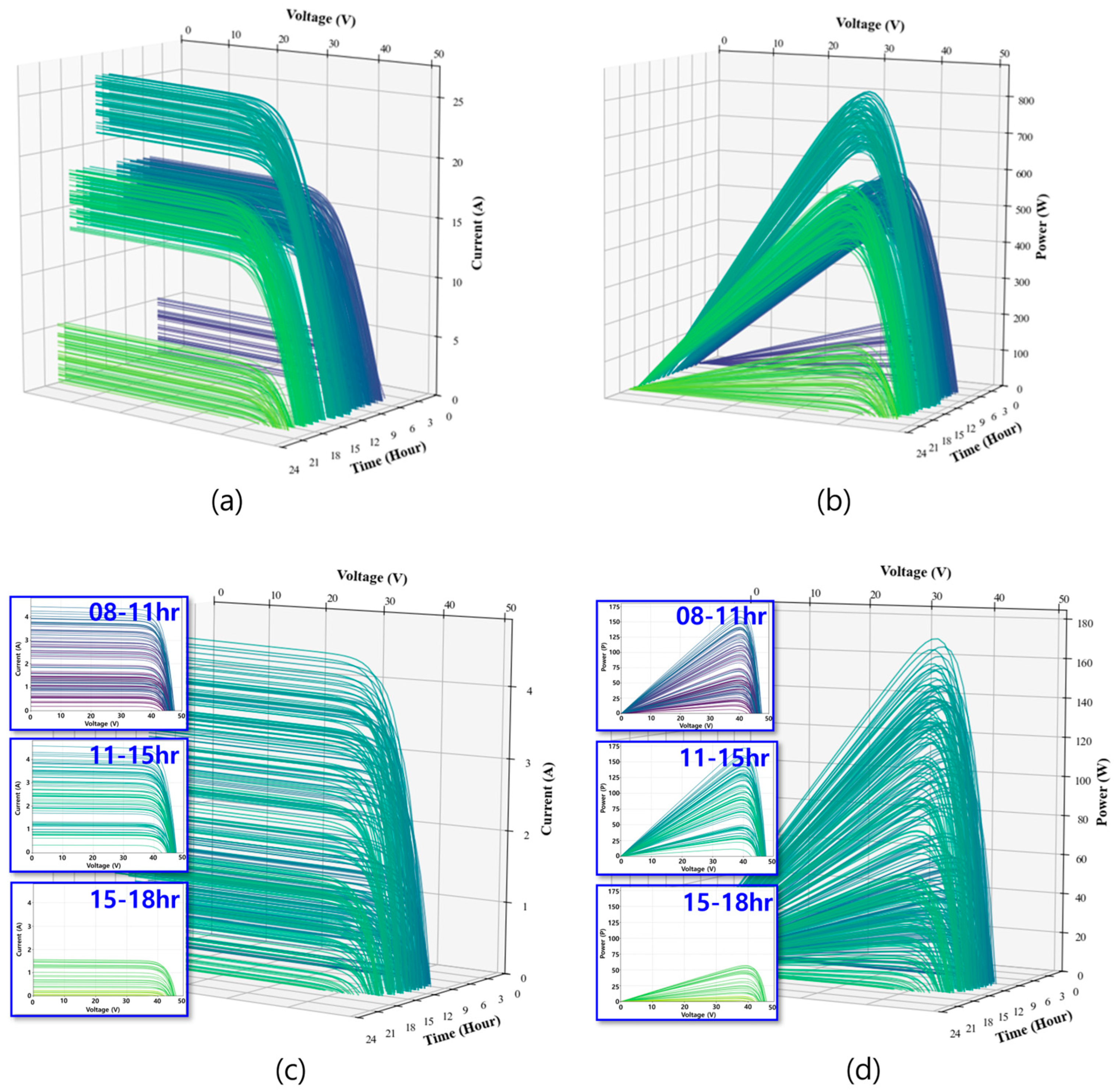
Figure 1. Simulated electrical characteristics of a solar panel for two distinct 30-day dataset. (a) I-V curves and (b) P-V curves for the high-yield spring climate dataset. (c) I-V curves and (d) P-V curves for the lower-yield winter climate dataset.
Sustainability 17 08538 g001
Figure 2. Internal structure of an LSTM cell.
Sustainability 17 08538 g002
Figure 3. Structure of an ESN.
Sustainability 17 08538 g003
Figure 4. Input time-series data for the two 30-day datasets used in this study: (a) Dataset A, characterized by stable spring climate conditions, and (b) Dataset B, representing more volatile winter climate conditions.
Sustainability 17 08538 g004aSustainability 17 08538 g004b
Figure 5. Power generation prediction using an LSTM for (a) the stable spring dataset and (b) the volatile winter dataset.
Sustainability 17 08538 g005
Figure 6. Power generation prediction using an ESN for (a) the stable spring dataset and (b) the volatile winter dataset.
Sustainability 17 08538 g006aSustainability 17 08538 g006b
Figure 7. Variation in the RMSE with the spectral radius and leaking rate for the ESN model.
Sustainability 17 08538 g007
Figure 8. Variation in the RMSE with the spectral radius and input noise for the ESN model.
Sustainability 17 08538 g008
Table 1. Comparison of model performance with previous studies on a normalized scale.
ReferenceModel UsedReported Performance (Normalized RMSE)
Al-Hajj et al. (2021) [42]LSTM0.082
Khan et al. (2022) [44]Hybrid CNN-LSTM0.075
Ullah et al. (2020) [43]LSTM0.090
This StudyLSTM0.072, 0.094
This StudyOptimized ESN0.0069, 0.0097
Disclaimer/Publisher’s Note: The statements, opinions and data contained in all publications are solely those of the individual author(s) and contributor(s) and not of MDPI and/or the editor(s). MDPI and/or the editor(s) disclaim responsibility for any injury to people or property resulting from any ideas, methods, instructions or products referred to in the content.