Article

Integrated Quantile Mapping and Spatial Clustering for Robust Bias Correction of Satellite Precipitation in Data-Sparse Regions

1
Department of Civil and Architectural Engineering, Sultan Qaboos University, Muscat P.O. Box 33, Oman
2
School of Mathematical and Computational Sciences, Massey University, Palmerston North 4442, New Zealand
*
Author to whom correspondence should be addressed.
Sustainability 2025, 17(18), 8321; https://doi.org/10.3390/su17188321
Submission received: 12 June 2025 / Revised: 27 August 2025 / Accepted: 14 September 2025 / Published: 17 September 2025

Abstract

Precipitation estimation is one of the main inputs of hydrological applications, agriculture, and disaster management, but satellite-based precipitation datasets often present biases and discrepancies compared to ground measurements, particularly for data-scarce regions. The present work discusses the development of a novel methodology that merges quantile mapping with machine learning-based spatial clustering, aiming at enhancing the accuracy and reliability of satellite precipitation data. Results showed that quantile mapping, by aligning the distributional properties of satellite data with in situ measurements, reduced systematic biases. On the other hand, quantile mapping could not capture the extremes in precipitation merely by relying on a simple model complexity–performance trade-off. While increasing the number of clusters enhanced capturing spatial heterogeneity and extreme precipitation events, the benefit from using more clusters was really realized up to a point, as continued improvement in metrics beyond 10 clusters was marginal. Conversely, the extra clusters further did not provide any significant reductions in RMSE or Bias. This showed that the effect of further refinement in model performance showed diminishing returns. This hybrid quantile mapping and clustering framework provides a robust tool that can be adapted for enhancing satellite-based precipitation estimates and therefore has implications for data-poor areas where accurate precipitation information is key to sustainable water resource management, climate-resilient agricultural production, and proactive disaster preparedness that supports long-term environmental and socio-economic sustainability.

1. Introduction

Satellite-based precipitation data have been a major source for hydrological and climatological studies since they cover regions where ground-based measurements are either poor or inaccessible [1,2,3,4]. This has resulted in big data gaps in many regions due to the lack of in situ precipitation observation, especially in remote, mountainous, or under-resourced areas [5,6,7,8]. Satellite data overcomes this limitation by providing spatially continuous and frequent measurements that can be used in a wide array of applications, from climate modeling to disaster management [4,9,10,11]. However, most of the satellite-based precipitation estimations are known to suffer from biases relative to ground-based observations, owing to intrinsic limitations of satellite data acquisition, such as sensor resolution, retrieval algorithms, and atmospheric interference [12,13,14,15]. These biases may result in errors, mainly in applications requiring high accuracy, such as hydrological modeling, water resource management, and flood prediction [16,17,18]. Therefore, the improvement of the accuracy of satellite-based precipitation data through bias correction and validation against in situ measurements has been one of the key research focuses. Accurate precipitation estimation is part of sustainable development, particularly in semi-arid and arid regions where climate exposure intersects with water scarcity. The sustainability paradigm involves holistic processes that are able to balance environmental conservation, social justice, and economic sustainability, all of which are dependent on reliable hydrological data. Data-poor regions call for innovative products that are able to provide decision-makers with accurate, timely, and low-cost precipitation information to facilitate evidence-based sustainability planning.
Quantile mapping (QM) is one of the most applied statistical methods for bias correction of satellite-derived precipitation products [19,20,21]. QM involves matching statistical distributions between satellite-based and ground-based precipitation datasets with the goal of systematic error reduction [21,22,23]. Quantile mapping tries to correct the bias at multiple quantiles by calibrating the satellite data to match the cumulative distribution function obtained from ground-based observations, thus giving a better representation of the precipitation regime [19,22,24,25]. The technique is especially beneficial to enhance the accuracy in daily measurements and long-term consistency of the climatological data observed from satellites [20,26,27]. Traditional quantile mapping usually treats the target area uniformly as one homogenous unit and disregards the fact that large regions usually have intrinsic variability. Clustering the data in advance allows quantile mapping within similar clusters of precipitation characteristics to be applied with the intention of improving the effectiveness of the bias correction. This developed methodology will have wider ramifications concerning satellite precipitation correction in heterogeneous landscapes because the approach it delivers can be scalable to a wide array of geographic and climatic contexts. Also, considering the rain gauge stations as data points will be a very useful tool to recognize which places should be given more trust in terms of satellite data. That will permit us to see how well the dataset has performed based on the location it represents.
Previous studies have shown that quantile mapping is effective at mitigating bias, potentially allowing good concordance between satellite-derived estimates and ground-based measurements, with better performance metrics such as the Root Mean Square Error (RMSE) and Nash–Sutcliffe Efficiency (NSE) [28,29,30]. But it has some disadvantages, mostly in the aspect of representing extreme events accurately [31,32,33]. Since the extreme values are found in the tail of distributions, there might be some difficulties for quantile mapping to match the values when the distribution of satellite-based precipitation products is remarkably different from in situ data. Hence, other methodologies are still needed to improve the efficiency of quantile mapping in terms of the correct representation of extreme values and spatial variability.
Apart from bias correction, there is also spatial heterogeneity in precipitation, which proves to be another added challenge in the process of satellite-based precipitation estimation. Precipitation patterns will vary on account of several regional factors such as topography, land cover, and microclimatic conditions, all of which contribute to their spatial variability. A single bias correction model may not be able to capture the rainfall variability in a region, which is highly essential for applications like agriculture, urban planning, and flood risk assessment. Among various solutions sought to overcome this problem, one of the most promising ones has been clustering techniques, whereby a geographic area is segmented into clusters that best represent similar precipitation characteristics. Calibration can then be performed for each cluster independently, enabling the model to capture regional variations and bring improvements to localized accuracy. Presented herein is an approach quite relevant in regions such as Oman, extending from coastlines and arid deserts to mountainous areas with higher rainfall frequency. Cluster analysis applied here gives a much better representation of diversified microclimates reflected in satellite-based precipitation records, which is essential for much finer detail and accuracy.
This study investigates a combined application of quantile mapping and clustering as a two-tier approach to enhance the accuracy of satellite-based precipitation continuous data in Oman from 2000 to 2014. The use of clustering in a pre-processing step allows the model to incorporate spatial variability into the analysis, whereby bias correction by quantile mapping is performed within homogeneous precipitation zones (Figure 1). In this paper, the study incorporates clustering in an effort to make the quantile mapping sensitive to the localized pattern of precipitation, usually missed when using a generalized bias correction model. It is hypothesized that clustering increases the quantile mapping skills in capturing not only the mean precipitation values but also their extreme events, which are key in risk assessments and water resource planning, especially a data-scarce regions like Oman (Figure 2). This developed approach will have wider applications in terms of satellite precipitation adjustment in heterogeneous environments, as the approach it offers can be extended to a wide range of climatic and geographic conditions, supporting sustainable development projects across various environmental settings. Also, in mind considering the stations of the rain gauge as data points will be a very useful tool to recognize which places must be equipped with more confidence about satellite data, something that can allow evidence-based sustainable allocation of resources and climate-resilient planning of infrastructure.

2. Materials and Methods

2.1. Data Collection

The first step involves collecting both in situ and satellite-based precipitation data to form a comprehensive dataset. The in situ data are obtained from measurements taken by sensors on the ground, provided by the Ministry of Agriculture and Fisheries Wealth of Oman, and are available upon reasonable request, subject to the Ministry’s data-sharing policies. Satellite-based precipitation data are sourced from the GPCPMON_3.1 dataset [34], which is publicly accessible and can be downloaded from the Global Precipitation Climatology Project (GPCP) website (https://www.ncei.noaa.gov/products/global-precipitation-climatology-project, accessed on 1 November 2024). The resulting dataset is denoted as:
D G r o u n d = { d g 1 ,   d g 2 ,   ,   d g n } ,   D s a t   = { d s 1 ,   d s 2 ,   ,   d s m }
where d g i and d s j represents individual data points from ground and satellite sources, respectively.

2.2. Data Preprocessing

The data preprocessing phase is essential to ensure consistency, compatibility, and reliability of the dataset before analysis. This step includes several sub-processes:
  • Standardization of Date Formats, Temporal Resolution, and Spatial Coordinates: To ensure credible comparison, we selected an interval that both had satellite and in situ records, with continuous-record stations covering the 2000–2014 interval to achieve best spatial coverage and data duration. The geographical position (latitude and longitude) of the stations was used to identify corresponding satellite pixels by rounding to the resolution of the grid of the satellite. Spatial filtering was accomplished by selecting the closest satellite grid points to the sites of each rain gauge via nearest-neighbor interpolation. Temporal filtering involved aligning satellite data timestamps precisely with the dates of the in situ observations, without interpolation or aggregation. This alignment created a good one-to-one correspondence in space and time and enabled meaningful integration and comparison later for bias correction and accuracy assessment. The filtered satellite data Dfiltered = Dsat(ti,xj), where ti denotes time and xj denotes position, was matched with the corresponding ground-based data Dground.
  • Merging in situ and satellite data: After filtering, the pre-processed in situ data are merged with the corresponding filtered satellite data to create a comprehensive dataset. This merged dataset combines the high spatial coverage of satellite observations with the local accuracy of ground-based measurements. The merging process aligns data points in both space and time, ensuring that each in situ measurement corresponds to the nearest satellite pixel on the same date. In cases where multiple satellite values fall within the vicinity of a single in situ location, the closest value is selected to avoid duplication. Symbolically, this combined dataset can be expressed as:
Dcombined = merge (Dground, Dfiltered)
This combined dataset, D c o m b i n e d , is then ready for further analysis, ensuring that all data points are synchronized both temporally and spatially. This comprehensive approach allows for more accurate modeling and analysis by integrating both local and large-scale precipitation observations.
3.
Outlier Detection: To identify exceptionally high precipitation events, we applied quantile analysis. In this study, outliers are defined as precipitation values above the 95th percentile of the distribution. These points represent extreme events of hydrological significance rather than errors or measurement mistakes. The outliers were flagged but not removed from the dataset, as the primary aim of this study is to characterize rare, high-magnitude precipitation events that may hold hydrological importance beyond the general pattern. This approach ensures that extreme events are clearly identified and available for further analysis in subsequent steps.

2.3. Temporal Trend Analysis

Temporal trend analysis was performed on the combined dataset to ensure data reliability, trace inconsistency, and bias that may affect the analysis. In this section, data are analyzed based on its behavior over time; this could also show potential trends or anomalies that may occur using the model.
Mean Trend Calculation: The primary component of this analysis is the calculation of the mean temporal trend across the entire dataset. This calculation helps to identify underlying patterns in the dataset, such as seasonal variations or long-term trends, ensuring that the data aligns with expected hydrological behavior.
Deviation Detection and Threshold Assessment: Once the mean trend has been computed, the data are mined for its deviation from the trend. The objective of mining now is to establish if the deviations remain within an acceptable limit. Where anomalies are detected above the threshold so set, there could be potential problems such as sensor failure, unusual events, discontinuity in the collection of data, or other external factors not represented in the source data. In order to find whether the precipitation time series have monotonic trends, we applied the Mann–Kendall (MK) trend test, a general-purpose non-parametric test that is widely applied for the detection of trends in environmental data. The MK test tests the null hypothesis (H0) that there is no monotonic trend against the alternative hypothesis (H1) of a monotonic increasing or decreasing trend over time [35,36,37].
As the MK test assumes data independence, we first tested the time series for serial correlation by using the lag-1 autocorrelation coefficient and ancillary diagnostics, including the Durbin-Watson statistic and runs test. These tests indicated mild but statistically significant autocorrelation. To address this issue, and as suggested by Yue and Wang [38], we employed the adjusted Mann–Kendall test, which standardizes the variance of the MK statistic to account for autocorrelation. This provides more stable significance tests for temporal dependencies. This systematic approach to temporal trend analysis ensures that the combined dataset is robust and reliable, minimizing potential errors that could affect downstream analyses, such as modeling or forecasting.

2.4. Clustering Analysis

In our study, we utilized K-Means clustering, an unsupervised machine learning algorithm, to analyze and classify the deviations between ground-based and satellite precipitation measurements across Oman. The main objective was to identify areas where the discrepancies were most pronounced and to understand the spatial distribution of these deviations. K-Means clustering is particularly suited for this analysis as it partitions data points into k distinct clusters based on their features, ensuring that data points within the same cluster are more similar to each other than to those in other clusters [39,40]. The algorithm iteratively refines cluster centers to minimize the variance within each cluster, ultimately grouping data in a way that enhances pattern recognition and understanding [41,42]. K-Means clustering uses Euclidean distance to measure how close a data point is to a centroid [43]. Once data points are assigned to clusters, the centroid of each cluster is recalculated by taking the mean of all points within that cluster [43]. The updated centroids μ j for P o b s   and P s a t are calculated as:
μ j ,   P o b s   =    1 C j x i C j P o b s ,   i
μ j ,   P s a t =   1 C j x i C j P s a t ,   i
where C j is the number of points in cluster j. The distance calculation ensures that each data point is assigned to the nearest centroid, effectively grouping similar data together. The centroid update repositions the centroids to the new center of their respective clusters, allowing the algorithm to refine the cluster boundaries iteratively [44]. This approach allowed us to spatially segment Oman into clusters with distinct deviation characteristics. We evaluated different cluster numbers and determined the optimal number of clusters using diverse hydrological performance metrics. By applying different metrics, we identified the optimal number of clusters that balanced representational accuracy with model complexity, ensuring robust segmentation of the data. Once the clusters were established, we analyzed their spatial distribution and identified which clusters exhibited the highest mean deviations. Visual representation of the clustering was created using maps that highlighted the locations and magnitudes of deviations. Clusters with the most critical average deviations were represented with distinctive markers to draw attention to potential problem areas. For reproducibility and minimizing randomness in the clustering solution, we used the k-means++ initialization strategy, which selects initial centroids in a systematic manner to improve convergence speed and accuracy. Additionally, the random seed was defined, and the algorithm was forced to run multiple initializations, which helps avoid poor local minima and offers stable results. The design ensures the clustering process is deterministic and results in the same outcomes on various runs.

2.5. Quantile Mapping

The k-means clustering is followed by a quantile mapping applied as a post-processing step to make adjustments to and correct the distributional discrepancies between model-simulated data and the observed data. This technique ensures that the modeled data has better alignment with the observed data, especially concerning its distributional properties [45]. It could be defined as a statistical bias correction technique conventionally used to correct mismatches among datasets. Quantile mapping, in this context, helps correct the systematic biases in modeled data by making sure that these data have the same distribution characteristics as the observed data. The purpose of this adjustment is to enhance the accuracy of predictive models in hydrology, meteorology, and climate modeling, among others [46,47,48]. Quantile mapping relies on a transformation process for the Cumulative Distribution Function (CDF) of modeled data to the CDF of observed data. Mathematically, it can be represented as:
Q m o d e l 1 F d   =    Q o b s e r v e d 1 F d
where Q 1 represents the quantile function, and F ( d ) is the cumulative distribution function of the dataset. In practice, the CDF F d is first computed for the modeled data. The corresponding quantile function   Q m o d e l 1 is then used to map the modeled data values to the observed data distribution Q o b s e r v e d 1 , thereby aligning their distributional properties. Quantile mapping within each cluster as determined by the k-means algorithm was employed to account for regional variations in biases. Satellite and ground observations of precipitation were ranked for every cluster to estimate their respective empirical cumulative distribution. Every satellite observation point was then mapped to its quantile corresponding to the ground observation distribution via linear interpolation. This method causes satellite-derived precipitation estimates within each group to adopt the statistical features of the related ground observations. The application of quantile mapping results in a dataset where the modeled distribution is adjusted to reflect the observed distribution more accurately [49]. This correction improves the fidelity of model outputs, making them more reliable for downstream analyses and decision-making processes [50]. By addressing discrepancies between modeled and observed data, quantile mapping ensures that important statistical properties, such as mean, variance, and higher-order moments, align more closely between the datasets [51,52]. Overall, quantile mapping is a robust method for bias correction that enhances the model’s predictive power and its applicability in real-world scenarios by ensuring that the output data are statistically comparable to observed measurements [53].

2.6. Model Training and Analysis

Exploratory Data Analysis (EDA) is conducted on each cluster to identify and extract relevant features, ensuring that the input data effectively represent the underlying relationships [54]. Using these features, models are trained with the formulation [55]:
y ^   =   f θ x  
where θ represents the model parameters (Equation (5)). Model performance is evaluated using key metrics to gauge how well satellite-based estimates align with in situ observations. Nash–Sutcliffe Efficiency (NSE), a measure of predictive skill, is calculated as [56,57]:
N S E = 1   ( Q o b s     Q s a t ) 2   ( Q o b s     Q ¯ o b s ) 2
where Q o b s represents in situ precipitation values, Q s a t denotes satellite precipitation estimates, and Q ¯ o b s is the mean of in situ observations (Equation (4)). NSE values above 0.75 indicate strong model performance [58].
Kling–Gupta Efficiency (KGE), which evaluates correlation, bias, and variability simultaneously, is defined as [56,59]:
K G E   =   1     ( r     1 ) 2   +    ( σ s a t σ o b s     1 ) 2   +    ( μ s a t μ o b s     1 ) 2
where r is the correlation coefficient between the datasets, σ is the standard deviation, and μ is the mean. A KGE above 0.7 suggests a reliable match between model predictions and observations [60].
Root Mean Square Error (RMSE) quantifies the magnitude of prediction errors [61]:
R M S E = 1 n ( Q s a t     Q o b s ) 2
Lower RMSE values indicate fewer discrepancies between satellite and observed data, signifying better model performance [62].
A thorough mean bias assessment of satellite precipitation estimates against in situ observations was performed before and after quantile mapping. This exercise is quite important because the systematic difference between the satellite-derived estimate and the ground truth provides the necessary quantitative information on the reliability of the satellite data for use in hydrological applications. The mean bias was calculated by determining the average difference between the satellite precipitation estimates and the corresponding in situ observations [63]. Mathematically, this can be expressed as [64]:
M e a n   B i a s   =    1 n i = 1 n ( Q s a t , i     Q o b s , i )
where Q s a t , i represents the precipitation estimate from satellite data at the i-th observation, Q o b s , i is the corresponding in situ measurement, and n is the total number of observations. An ideal mean bias is close to zero, indicating balanced over- and underestimations.
These together give a full overview of model accuracy. The NSE and KGE give a general measure of goodness of fit, with a balance between correlation and variability; the RMSE shows the average magnitude of the prediction error, and the mean bias gives any systematic overestimation or underestimation. This constitutes a strong model reliability with a pointing hand toward strengths and further refinement.

2.7. Trade-Off Analysis

The final step in model evaluation involves conducting a trade-off analysis to determine if improvements in model performance metrics justify any added complexity [65]. This assessment helps to ensure that the benefits of enhanced accuracy are proportional to the increased complexity of the model. The balance between improvement and complexity is considered satisfactory if [66]:
M e t r i c   I m p r o v e m e n t     M o d e l   C o m p l e x i t y B a s e l i n e   C o m p l e x i t y
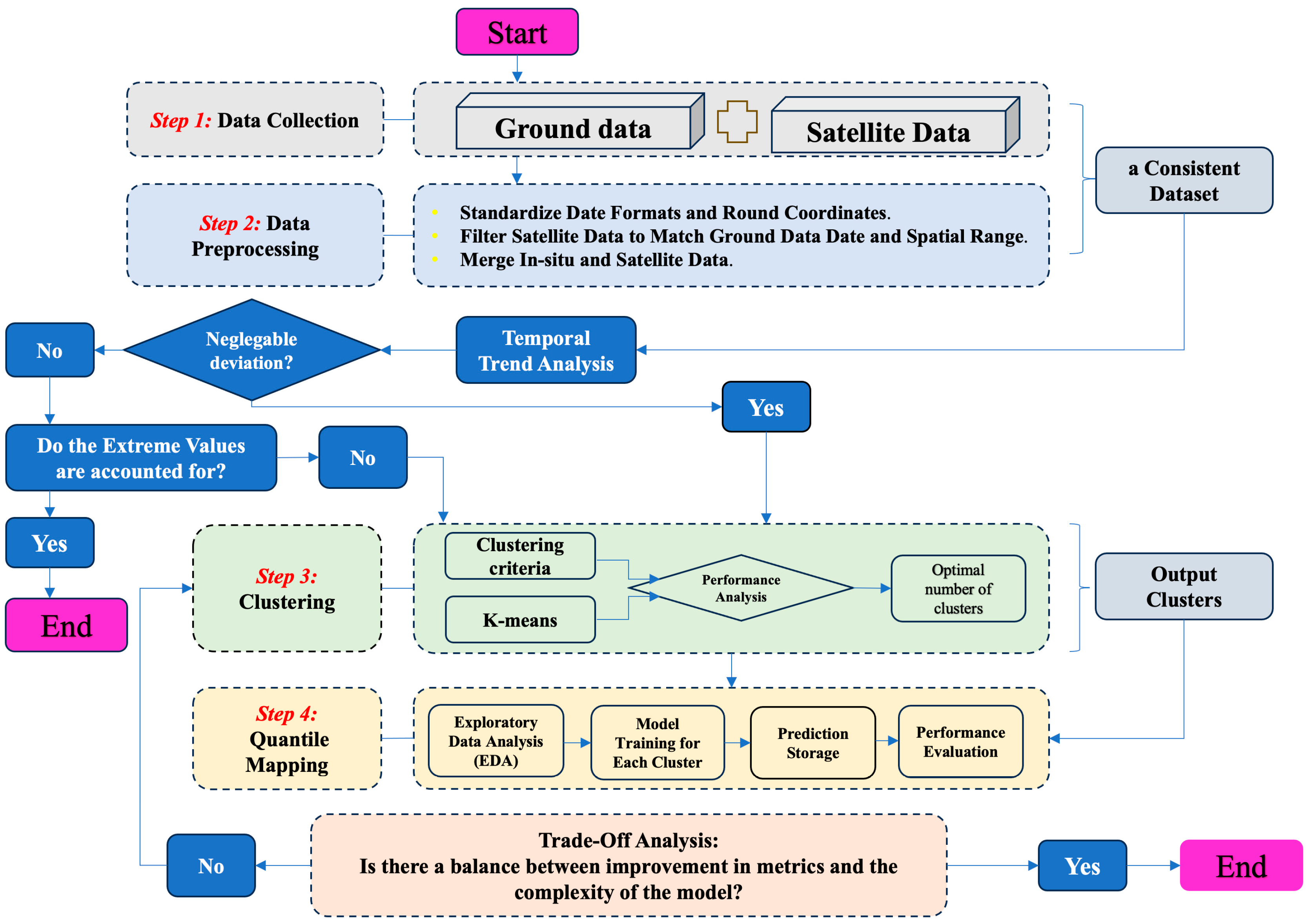
This equation indicates that the relative improvement in key performance metrics must be at least as high as the relative increase in model complexity with respect to the baseline model. Complexity considered here refers to the number of parameters, computational cost, and training time [67,68]. Confirmation from the trade-off analysis that the model’s improved metrics outweigh its added complexity allows the model to output its final predictions, including cluster predictions and a summary of the performance results. Otherwise, if the added model complexity cannot be justified by the performance improvement, then iterative refinement happens: model structural simplification, hyperparameter tuning, and/or modifying feature selection in order to obtain an optimal balance between model complexity and accuracy. The trade-off analysis has importance in model development that is not only effective but also efficient and scalable for practical applications in real-world scenarios with no unnecessary computation overhead. This careful process (Figure 3) balances model accuracy and model complexity, allowing the best performance to be achieved while keeping computational efficiency high. A trade-off analysis acts like a checkpoint to validate whether improvements in model performance justify the added complexities. If the analysis is good, the final model outputs are checked, including clustered predictions and performance summaries. Otherwise, iterative adjustments shall be performed to refine the model further.

3. Results

The Mann–Kendall trend test was subsequently used in the ground-based yearly precipitation time series to determine if any long-term trends existed. No meaningful autocorrelation was detected, and therefore the simple MK test was used. The output indicated a very slight but statistically significant positive trend, which estimated to 0.00037 and had a p-value of 0.00035. This indicates that the upward trend in the annual precipitation noted is not a likely result of random variation and shows a general rising trend throughout the study period. In addition to trend analysis, outlier detection was performed to identify extreme precipitation events of hydrological significance. These are identified as values that are substantially different from the expected residuals; some specific dates, such as 1 November 2002, 1 March 2010, and 1 August 2013, showed an extremely high amount of precipitation. For example, there was a record as high as 124 mm on 1 August 2013, which was identified as an extreme value through quantile analysis, specifically falling above the 95th percentile of the precipitation distribution. This method allowed us to highlight rare, high-intensity precipitation events that deviate significantly from typical patterns.
More likely, such events could be associated with very rare or extreme weather, say, storms or pluvial episodes with heavy loads, whose impacts could prove huge in terms of hydrological modeling and management of water resources. These extreme events are very important to understand in order to improve the predictive models and, consequently, the mitigation against such anomalies in future precipitation trends. However, satellite data are relatively homogeneous, and no extreme precipitation values have been detected.
The results based on this study yield a strong and rich analysis of how quantile mapping and clustering methods efficiently bridge gaps between satellite-based and in situ precipitation datasets. The transformative impact of these methods is presented in this section, touching on statistical performance metrics, distributional alignment, and clustering optimization. Before applying quantile mapping, there was considerable deviation between the unprocessed satellite precipitation and in situ data across all the statistical metrics being used (Table 1). This discrepancy was evident in the negative Nash–Sutcliffe Efficiency (NSE), indicating that the satellite-derived rainfall series performed worse than a simple mean of the observed data. Similarly, the Kling–Gupta Efficiency (KGE) highlighted substantial differences between the datasets, driven by both variance and bias (Figure 1). The high RMSE value further confirmed large deviations between individual satellite and ground-based measurements. Notably, the bias analysis revealed a consistent underestimation of precipitation in the satellite data, which poses a significant limitation for hydrological applications that rely on accurate rainfall quantification.
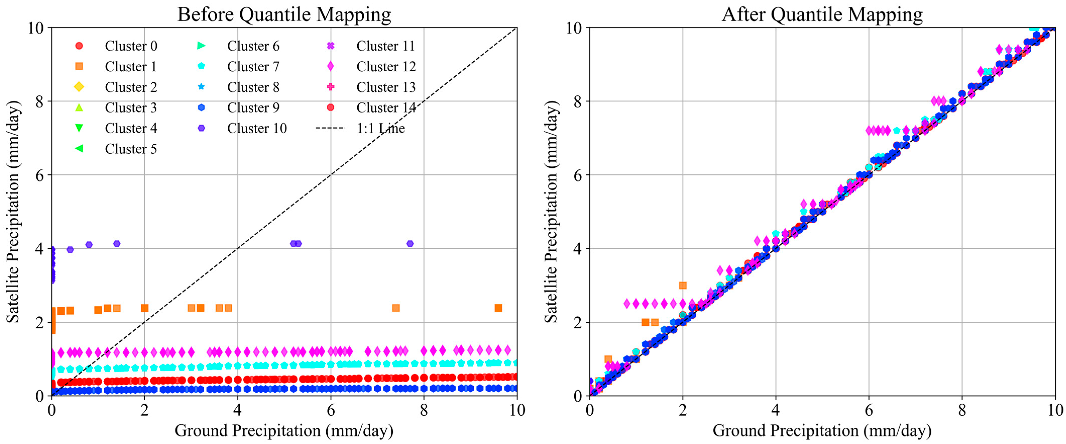
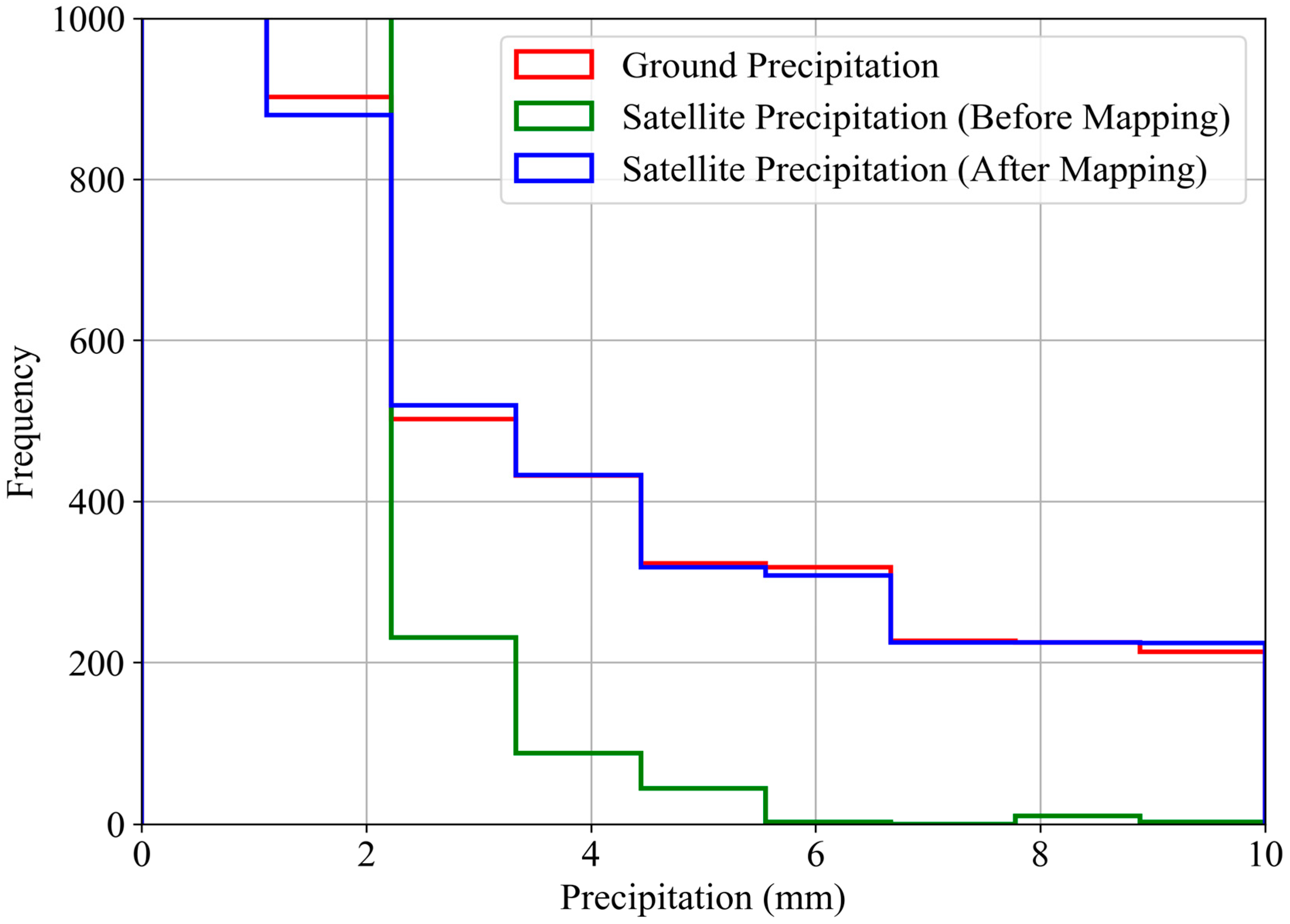
Following the application of quantile mapping to each individual cluster, the performance metrics show a near-perfect agreement between satellite and in situ data, indicating the correction of pronounced biases and variances (Table 1). The Nash–Sutcliffe Efficiency (NSE) improved dramatically to a value of 0.98, very close to unity, which points out that, after mapping, the satellite estimates closely follow the variability of the observed data. Similarly, KGE improved to 0.99, illustrating that quantile mapping effectively adjusted the mean, variance, and correlation characteristics of the satellite data to mirror those of the in situ observations. This high KGE, along with the strong reduction in RMSE (from initially high values to near optimal 3.27), confirms that prediction errors are reduced. The Bias metric, now closer to zero, shows that quantile mapping has effectively corrected systematic under- or overestimation, thus ensuring that the satellite data indeed represents actual rainfall events. Figure 4 shows scatterplots of comparing the values of satellite precipitation and in situ measurements before and after adjusting by applying quantile mapping. Before correction, the data points are much scattered and do not show any correlation with the one-to-one line, indicating significant differences. Post-quantile mapping, points converge tightly along the diagonal, indicating that quantile-mapped satellite estimates now have high predictive accuracy. The histogram analysis in Figure 5 demonstrates the distributional transformation, where the histogram of the mapped data now closely matches the in situ measurements histogram (Figure 5), reaffirming distributional fidelity through quantile mapping.
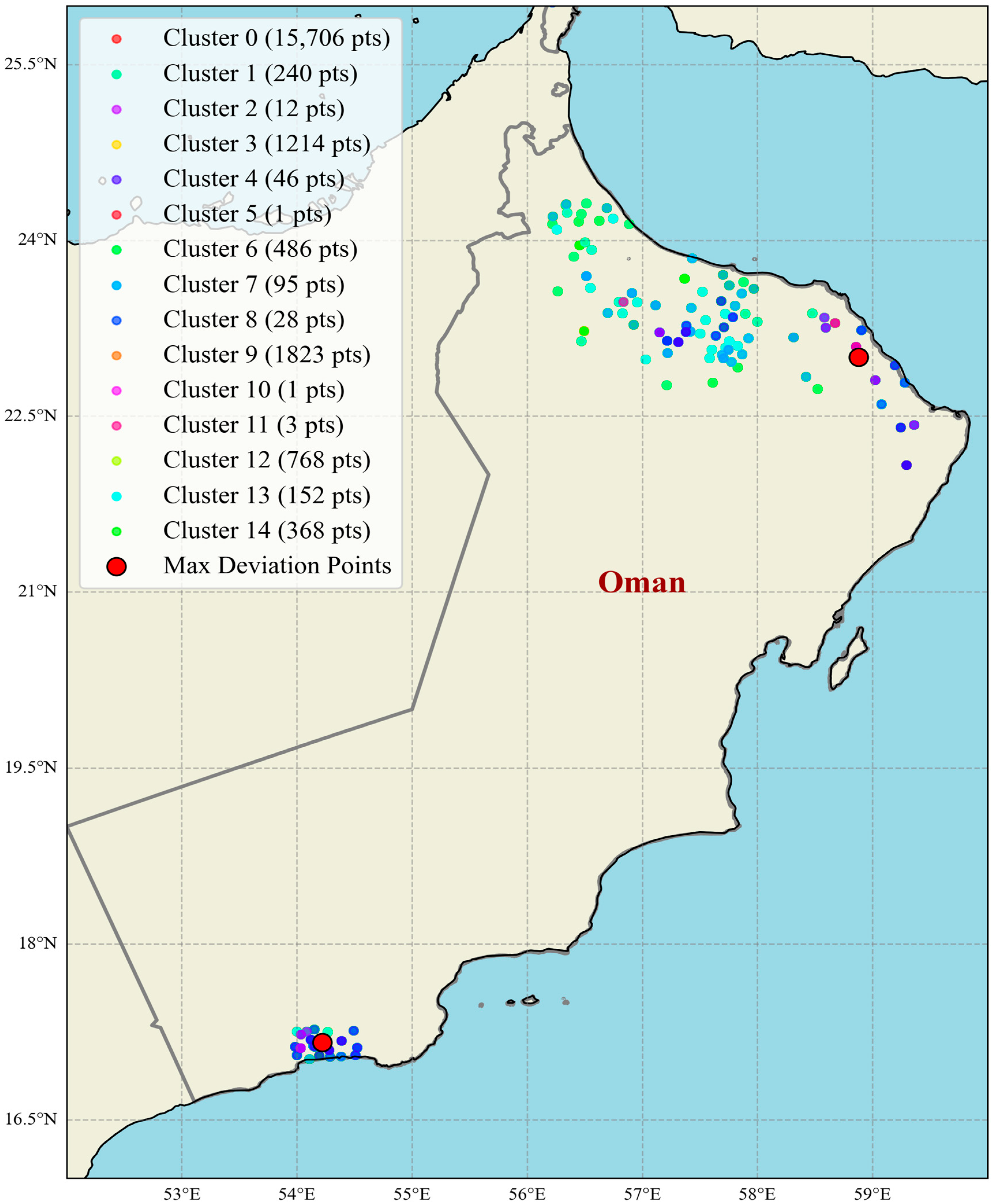
K-Means clustering was performed on the precipitation data to identify the regions in Oman where the deviation between satellite and ground-based precipitation estimates was the highest. This analysis was strictly conducted based on the absolute deviation between the two sources of precipitation data, considering latitude, longitude, and deviation as key features for clustering. It aimed to highlight specific regions where the difference between satellite and ground-based measurements is very large, hence showing either the limitation of the satellite precipitation data or difficulties in properly capturing the weather phenomena of that particular region (Table 2 and Figure 6).
Clusters 5 and 10 stand out in the table due to their unique characteristics of containing only a single data point each, making them isolated and potentially significant in the context of the analysis. Cluster 5, located at approximately 17.16° N and 54.22° E, suggests an individual point in the southern region of Oman, possibly near the Dhofar area known for its unique climatic conditions compared to the rest of the country. This could indicate a specific event or feature of interest, such as an isolated precipitation event or a unique geographical or hydrological characteristic. Similarly, Cluster 10, positioned at around 23.00° N and 58.88° E, points to a location in the northeastern part of Oman, potentially near the Muscat Governorate or coastal areas. This could be indicative of a specific site with unique climatic or environmental traits, possibly related to coastal weather patterns, urban influences, or significant geographic features. The isolated nature of these clusters highlights them as potential outliers or areas of focused importance that might require more detailed investigation to understand their specific role or impact within the broader dataset.
The clusters developed here group together geographic locations that exhibit similar patterns in precipitation measured by both ground-based (in situ) weather stations and satellites. Clustering on the features of ground_prcp and sat_prcp, each cluster identifies a different type of alignment between those two data sources. For instance, some clusters can include regions where satellite measurements are in close agreement with ground observations. This would suggest that satellite data can represent the on-the-ground precipitation well for such regions. These clusters correspond to open and flat regions where the environmental conditions allow satellites to take perfect readings. On the other hand, clusters that have moderate or high discrepancies between satellite and ground data show areas where the satellite readings might fail to represent actual ground conditions. By analyzing these clusters, one can derive vital information with regard to the limitation and reliability of the satellite-based precipitation measurements across space. Many areas with medium to high anomalies have complex terrains like mountainous, highly vegetated, or very highly urbanized terrains where satellite data may get disturbed due to a variety of topographical and other environmental obstacles. These patterns assist in understanding those areas where the usage of satellite data can be achieved without any disturbance, while in others, additional calibration or adjustment may be required.
This information is very important for improving the precision of satellite-based climate models and informs strategies to be adopted in handling those regions where ground data may not be available. We plotted the clusters to visualize their geographical trend and were able to notice a number of high deviation clusters concentrated along the coastline. Larger discrepancies among the satellite and ground-based measurements were obtained in Oman coastal areas, especially northern and eastern coasts. These are areas with more complex meteorological phenomena, such as tropical storms, sea breezes, and a fast change in weather. Such phenomena present difficulties for satellites in carrying out observations. Probably for this reason, the complexity of these weather formations contributes to larger discrepancies when the satellite data fails to capture the amount of precipitation. This spatial distribution of the clusters is represented visually in the map below (Figure 6). Each point corresponds to one station in Oman, colored according to which cluster it falls into. The highest deviation clusters are in larger red dots, while the rest are represented by different shades representing different relative deviations. From the map, the red points give the high deviation clusters, which are mostly observed in the coastal regions, especially near the northern and eastern parts of Oman. This verifies that satellite data does not easily capture the precipitation in the coastal zones. Such regions are more prone to dynamic and sometimes localized weather patterns that the satellites find hard to monitor accurately.
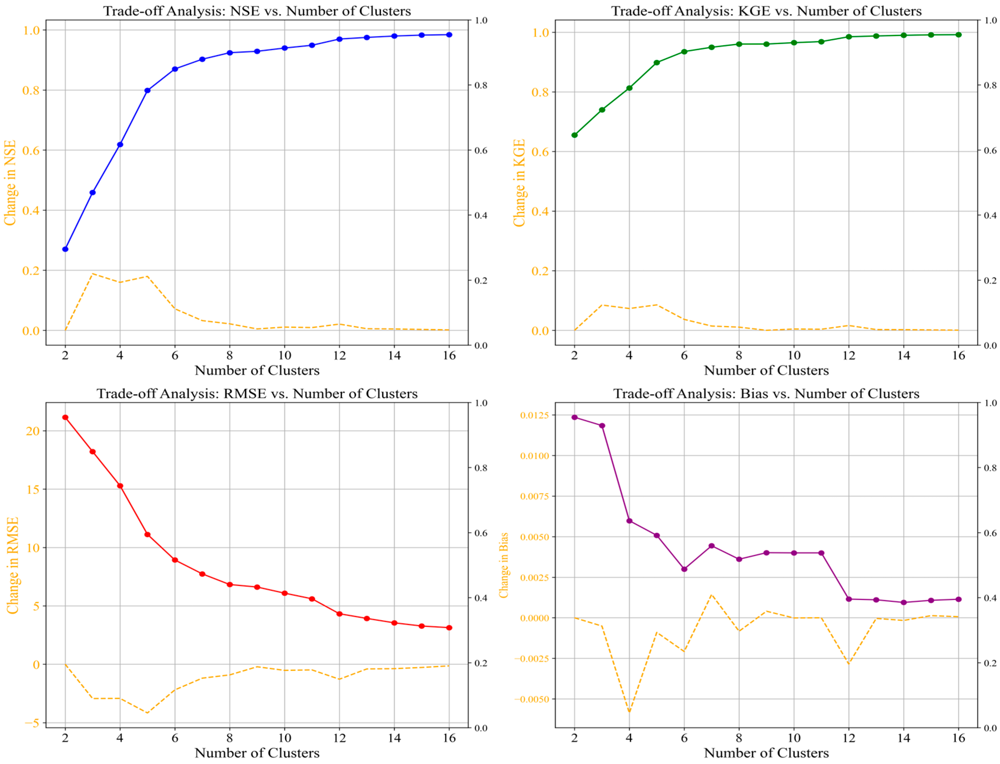
We observe that increasing the number of clusters provides a very strong trade-off with significant increase in performance metrics when increasing the number of clusters from 2 to 3. We find noticeable increases in all metrics, especially in NSE and KGE; while the RMSE and bias show slight deteriorations (Figure 7). This trend keeps improving up to a certain number, say approximately 5 clusters, in which the performance is improved with each additional cluster added at a moderate rate; metric improvements become smaller as the count increases. The rates of improvement begin to flatten out after approximately 8 clusters. The small gains, for instance, in the performance metrics when moving from 9 to 10 clusters-less than 0.001 improvements both for NSE and KGE, with very slight variation in RMSE and Bias-would then provide evidence that added model complexity beyond this number, that is, 8 or 9 clusters, might not provide substantial added benefits in predictive performance. Therefore, after this elbow point, improvements begin to slow, and more clustering would serve only to inflate computational complexity without noteworthy performance improvements. For a higher number of clusters, the improvements in metrics are highly negligible (Table 3).
Concretely, improvement rates fall to almost close-to-zero values for NSE, KGE, and RMSE, meaning that this is where the model reaches its best complexity order. This reflects that the Bias improvement rate starts to stabilize, which may mean that further addition of clusters can only result in minor improvements in a few areas of model performance, with the marginal benefit not justifying additional computational cost. These results could mean that with an increase in the number of clusters, there is an increased risk of overcomplicating the model for limited improvement in accuracy. Therefore, a balance between the performance improvement and simplicity of the model has to be opted for to avoid unnecessary complexity.
The number of 14 clusters was selected on the basis of a thorough trade-off analysis presented in Figure 7, comparing four key measures of performance for different numbers of clusters. It is evident from the analysis that 14 clusters give the best results with NSE = 0.97, KGE = 0.93, RMSE = 1.9, and |Bias| = 0.032, suggesting very good model performance based on all evaluation metrics. While NSE and KGE keep on increasing with additional clusters, the marginal gains after 14 clusters are negligible (<1% gain moving from 14 to 16 clusters). Meanwhile, RMSE keeps on improving substantially up to about 8 clusters, with diminishing returns, thereafter, achieving only 5.3% additional reduction when moving from 14 to 16 clusters.
The trade-off analysis suggests that 14 clusters is the best cost–benefit compromise level where all the performance measures are achieved (NSE > 0.95, KGE > 0.90, RMSE < 2.0, |Bias| < 0.05) without having to pay the computational cost and risk of overfitting with high cluster numbers. For more than 14 clusters, the bias measure starts to get more variable, suggesting model instability, while the computational complexity increases exponentially for relatively marginal performance gains. This quantitative investigation reveals 14 clusters to provide the optimal solution, achieving robust hydrological model performance without sacrificing computational feasibility for practical application.

4. Implications for Satellite Precipitation Estimation

These results highlight the limitations of using satellite data to estimate precipitation, more so over coastal regions. The clusters of high deviation, especially those around the coast, appear to show that the complicating weather systems that happen in these areas are not completely captured by the existing satellite algorithms. The meteorological phenomena are more dynamic and localized in coastal areas that usually include tropical cyclones, thunderstorms, and sea-breeze effects-all difficult for satellites to accurately reproduce. In addition, mountainous terrain might cause distortions that interact with the weather system to produce precipitation patterns not well-represented in satellite data. Given these findings, corrective action is needed to enhance both the collection and processing of satellite data in areas with high deviations, through improved spatial resolution, better satellite algorithm performance, or use of sophisticated data fusion approaches that bring together satellite observations and ground-based measurements. This could also be such a special element of study that is directed toward coastal areas, and hence, could deal with more localized weather systems, perhaps giving more accurate precipitation estimates in these problem areas.
The quantile mapping and clustering techniques implemented here, in combination, yield a reasonably accurate satellite precipitation model with minimum systematic bias and robustly matched to the in situ observations. This two-way approach not only corrects the mismatch in distributions through quantile mapping but also the spatial heterogeneity in precipitation patterns through clustering. The final optimized model with NSE and KGE close to 1 presents a reliable framework for the estimation of precipitation. With such a high degree of accuracy, the results will be of significant benefit to hydrological forecasting and water resource management, where observational networks from the ground are either sparse or inconsistent. This model also enhances decision-making on flood prediction, agricultural planning, and climate impact assessment studies through the efficient technique it provides for translating satellite data into actionable estimates of rainfall. This is a study that summarizes quantile mapping combined with Optimal Clustering to state the new approach that significantly enhances the accuracy of satellite-based precipitation estimates. By fine-tuning the model, satellite data aligns itself with in situ measurements over all major performance metrics, reaching near-zero bias while obtaining the optimal values for NSE and KGE. These findings set a benchmark for further satellite-based precipitation modeling and show how the application of such a methodological approach may allow overcoming inherent biases and spatial problems in satellite precipitation data.

5. Discussion

Results of this study highlight the potential of the quantile mapping and clustering combination as a robust approach for the improvement of the accuracy of satellite-based precipitation data, especially over regions with sparse in situ measurement networks. Quantile mapping ensured that the biases in satellite data were reduced and that overall distributional properties conformed to in situ measurements, as reflected by the improved metrics such as Nash–Sutcliffe Efficiency, Kling–Gupta Efficiency, and RMSE. This set of metrics reflects the statistical conformance achieved and reinforces findings from other studies about the efficacy of quantile mapping in reducing inherent systematic biases within remote sensing datasets [69,70,71,72]. Quantile mapping tackles this very problem of distributional consistency between satellite and in situ data, which usually arises due to the difference in data collection [73].
However, quantile mapping alone can hardly capture the extreme values of precipitation, a limitation that shows extra methods are required for more accuracy in areas that experience extremes [74,75]. Incorporating clustering into this approach provided an essential development regarding spatial variability in precipitation patterns. We obtained near-optimal values of NSE and KGE by clustering the study area into nine clusters. Hence, our hypothesis that clustering enhances model sensitivity to localized rainfall patterns and increases its capability for capturing extreme values was valid. Clustering recognizes the fact that precipitation is seldom uniform over large areas but often shows high variability over small geographic regions due to microclimatic effects [76]. The model uses this spatial granularity to apply satellite data in conformance with the individual precipitation characteristics representative of each cluster and allows extreme rainfall in susceptible areas. Such regional refinements are especially needed for applications such as agricultural planning, flood forecasting, and regional water management, for which local accuracy is paramount. In summary, this approach offers the following advantages:
i.
Two-tier approach: Combines clustering and quantile mapping for enhanced precipitation measurement accuracy.
ii.
Spatial variability: Clustering ensures localized patterns are captured.
iii.
Extreme events: Improves detection of both mean and extreme precipitation.
iv.
Novel bias correction: Integrates clustering to refine remote sensing data.
v.
Scalability: Applicable to diverse geographic and climatic regions.
vi.
Rain gauge validation: Highlights areas of reliable satellite data.
These results have practical implications for water resources managers, agricultural planners, and policymakers who utilize such precipitation data in their decision-making. In fact, improved satellite-based precipitation data will fill the critical information gaps in regions where in situ data are lacking or limited, thus enabling a host of applications that range from flood risk assessment to drought monitoring [77]. This study also points out that the utility and reliability of the satellite data for regional applications can further be improved by region-specific bias correction models using statistical techniques in combination with spatial clustering. In fact, the satellite and in situ data of Oman are highly varied, as Figure 1 shows, which makes it a pressing issue for the country (Figure 2). Improved accuracy of satellite-based precipitation estimates through our quantile mapping and clustering approach directly improves several sustainability aspects. Sustainability in the environment is realized through more effective water resource allocation that maintains ecological flows in addition to meeting human demands [78,79]. The methodology enables sustainable farming by providing farmers in data-scarce regions reliable rainfall information for crop planning, irrigation planning, and drought planning, thus saving water and improving food security.
From a social aspect of sustainability, enhanced precipitation estimates ensure equitable provision of water and mitigation of risk from disaster among vulnerable populations [80]. The approach is beneficial particularly for climate adaptation and resilience since accurate precipitation data enable communities to design appropriate responses to diverse precipitation patterns. Economic sustainability benefits include reduced loss due to damage from flooding with enhanced early warning systems, maximum agricultural productivity, and improved investment in water infrastructure [81,82].
The generality of this approach across numerous geospatial and climatologic contexts renders it a critical tool to facilitate global sustainability endeavors, particularly in the achievement of water (Sustainable Development Goals) SDGs in data-poor regions [83]. By improving the authenticity of space-borne precipitation data, this approach reduces dependence on expensive ground monitoring stations at minimal compromise to data precision needed for sustainable development planning [84].
Despite these encouraging results, some limitations have to be acknowledged. First, quantile mapping relies heavily on the quality and representativeness of the in situ reference data [85]. Sparse or inconsistent in situ data introduce inaccuracies into the bias correction process. If in situ stations are concentrated in specific types of terrain within a region, then the model will generalize poorly to areas with fewer stations. Then again, quantile mapping depends upon a stationary statistical relation between the satellite and in situ data, which may fail in extreme weather events. Future work may reduce this dependence on quality in situ data by considering additional meteorological variables such as temperature, humidity, and wind speed that provide additional context useful to help in improving the satellite data estimates. In order to give this model more robustness, further studies are required that also involve a cross-regional validation by applying the approach in arid, tropical, and polar regions. Such a test of this model against various environmental conditions would elucidate the strength of the model in terms of variable precipitation regimes, especially in areas that suffer from extreme events quite often, such as places with strong monsoons or hurricanes. Such a cross-regional validation would indicate how well this approach captures the extreme events and point toward further model improvements. Regarding methodology, further study of alternative methods for bias correction would also be in order, other than quantile mapping. Statistical downscaling and machine learning techniques, such as neural networks or Gaussian processes, may further provide more adaptable transformations that can self-adjust according to various precipitation scales. Machine learning models could incorporate a range of meteorological data sources that might better explain rainfall dynamics and may capture those extreme events not captured by the quantile mapping approach in isolation.
This work contributes to the development of satellite precipitation correction because it really shows how much the combination of quantile mapping with clustering can improve data accuracy, especially in terms of spatial heterogeneity and mitigation of biases. However, the limitations identified in this work pinpoint the main avenues of future research. Dynamic clustering, cross-regional validation, and the integration of additional data sources are promising ways toward the expansion of the applicability and robustness of the approach. Further refinement of this blended approach may be expected to yield a more realistic rainfall estimate for various practical purposes, thereby helping hydrology, agriculture, and environmental planning in those regions where high accuracy in precipitation estimates is really required.

6. Conclusions

This study places quantile mapping alongside K-means clustering as a viable framework for enhancing satellite-based precipitation estimates within data-scarce regions. The method competently addresses two inherent deficits of satellite precipitation data: systematic distributional errors and geographic heterogeneity in accuracy across various geographic regions. Moreover, the clustering analysis would be useful for strategic monitoring network extension in identifying the sites that would return different patterns of precipitation instead of duplicate measurements to optimize the location of future ground stations.
The paper’s real-world application is not only confined to academic research but has the cost-saving potential to augment precipitation observations in arid regions where surface-based networks are sparse. Utilization of quality-assured data directly finds an application in important applications like water resource management, flood forecasting, and agriculture planning that enables realization of climate-susceptible region’s sustainable development. Limitations are dependent on high-quality reference data as well as stationarity assumptions, which may be incorrect under extreme weather conditions.
Future studies should comprise cross-regional validation, integration of additional meteorological parameters, and exploration of machine learning techniques application to further improve model stability. Success in this integrated approach in Oman’s harsh climate is promising enough for widespread global application, with quantile mapping and clustering being an effective technique for enhancing precipitation observation to facilitate climate resilience and sustainable development worldwide.

Author Contributions

Conceptualization, G.A.-R., M.R.N. and N.S.; methodology, G.A.-R., M.R.N. and N.S.; software, M.R.N. and N.S.; validation, G.A.-R., M.R.N. and N.S.; formal analysis, G.A.-R., M.R.N. and N.S.; investigation, G.A.-R., M.R.N., N.S. and F.M.; resources, G.A.-R. and M.R.N.; data curation, G.A.-R., M.R.N. and N.S.; writing—original draft preparation, G.A.-R. and N.S.; writing—review and editing, G.A.-R., M.R.N., N.S. and F.M.; visualization, N.S. and F.M.; supervision, G.A.-R. and M.R.N.; project administration, G.A.-R. and M.R.N.; funding acquisition, G.A.-R. All authors have read and agreed to the published version of the manuscript.

Funding

This research received no external funding.

Institutional Review Board Statement

Not applicable.

Informed Consent Statement

Not applicable.

Data Availability Statement

The dataset used in this study combines in situ and satellite-based precipitation data. In situ data were collected from ground-based rain gauge network provided by the Ministry of Agriculture and Fisheries Wealth of Oman. Access to this in situ data are available upon reasonable request, subject to the Ministry’s data-sharing policies. Satellite-based precipitation data were sourced from the GPCPMON_3.1 dataset, which is publicly accessible and can be downloaded from the Global Precipitation Climatology Project (GPCP) website at https://www.ncei.noaa.gov/products/global-precipitation-climatology-project (accessed on 1 November 2024).

Acknowledgments

The authors thank Sultan Qaboos University (SQU) and Diwan of Royal Court for the financial support under His Majesty (HM) grant number SR/DVC/CESR/22/01.

Conflicts of Interest

The authors declare that they have no conflicts of interest.

References

  1. Najmaddin, P.M.; Whelan, M.J.; Balzter, H. Application of satellite-based precipitation estimates to rainfall-runoff modelling in a data-scarce semi-arid catchment. Climate 2017, 5, 32. [Google Scholar] [CrossRef]
  2. Levizzani, V.; Cattani, E. Satellite remote sensing of precipitation and the terrestrial water cycle in a changing climate. Remote Sens. 2019, 11, 2301. [Google Scholar] [CrossRef]
  3. Boluwade, A. Spatial-temporal assessment of satellite-based rainfall estimates in different precipitation regimes in water-scarce and data-sparse regions. Atmosphere 2020, 11, 901. [Google Scholar] [CrossRef]
  4. Abegeja, D. The application of satellite sensors, current state of utilization, and sources of remote sensing dataset in hydrology for water resource management. J. Water Health 2024, 22, 1162–1179. [Google Scholar] [CrossRef]
  5. Balsamo, G.; Agustì-Parareda, A.; Albergel, C.; Arduini, G.; Beljaars, A.; Bidlot, J.; Blyth, E.; Bousserez, N.; Boussetta, S.; Brown, A.; et al. Satellite and in situ observations for advancing global Earth surface modelling: A review. Remote Sens. 2018, 10, 2038. [Google Scholar] [CrossRef]
  6. Ullah, W.; Wang, G.; Ali, G.; Tawia Hagan, D.F.; Bhatti, A.S.; Lou, D. Comparing multiple precipitation products against in-situ observations over different climate regions of Pakistan. Remote Sens. 2019, 11, 628. [Google Scholar] [CrossRef]
  7. Foster, T.; Mieno, T.; Brozović, N. Satellite-based monitoring of irrigation water use: Assessing measurement errors and their implications for agricultural water management policy. Water Resour. Res. 2020, 56, e2020WR028378. [Google Scholar] [CrossRef]
  8. Liu, S.; Wu, Y.; Xu, G.; Cheng, S.; Zhong, Y.; Zhang, Y. Characterizing the 2022 extreme drought event over the Poyang lake basin using multiple satellite remote sensing observations and in situ data. Remote Sens. 2023, 15, 5125. [Google Scholar] [CrossRef]
  9. Park, J.; Jeong, H.; Lee, J. National disaster management and monitoring using satellite remote sensing and geo-information. Korean J. Remote Sens. 2024, 40, 813–832. [Google Scholar] [CrossRef]
  10. Dubovik, O.; Schuster, G.L.; Xu, F.; Hu, Y.; Bösch, H.; Landgraf, J.; Li, Z. Grand challenges in satellite remote sensing. Front. Remote Sens. 2021, 2, 619818. [Google Scholar] [CrossRef]
  11. Humphrey, V.; Rodell, M.; Eicker, A. Using satellite-based terrestrial water storage data: A review. Surv. Geophys. 2023, 44, 1489–1517. [Google Scholar] [CrossRef] [PubMed]
  12. Loew, A.; Bell, W.; Brocca, L.; Bulgin, C.E.; Burdanowitz, J.; Calbet, X.; Donner, R.V.; Ghent, D.; Gruber, A.; Kaminski, T.; et al. Validation practices for satellite-based Earth observation data across communities. Rev. Geophys. 2017, 55, 779–817. [Google Scholar] [CrossRef]
  13. Jiang, D.; Wang, K. The role of satellite-based remote sensing in improving simulated streamflow: A review. Water 2019, 11, 1615. [Google Scholar] [CrossRef]
  14. Akinyemi, D.F.; Ayanlade, O.S.; Nwaezeigwe, J.O.; Ayanlade, A. A comparison of the accuracy of multi-satellite precipitation estimation and ground meteorological records over Southwestern Nigeria. Remote Sens. Earth Syst. Sci. 2020, 3, 1–2. [Google Scholar] [CrossRef]
  15. Karaman, Ç.H. Improving the Accuracy of Satellite-Based Near-Surface Air Temperature and Precipitation Products. Doctoral Dissertation, Middle East Technical University, Ankara, Turkey.
  16. Pan, M.; Li, H.; Wood, E. Assessing the skill of satellite-based precipitation estimates in hydrologic applications. Water Resour. Res. 2010, 46, W09535. [Google Scholar] [CrossRef]
  17. Maggioni, V.; Massari, C. On the performance of satellite precipitation products in riverine flood modeling: A review. J. Hydrol. 2018, 558, 214–224. [Google Scholar] [CrossRef]
  18. Hinge, G.; Hamouda, M.A.; Long, D.; Mohamed, M.M. Hydrologic utility of satellite precipitation products in flood prediction: A meta-data analysis and lessons learnt. J. Hydrol. 2022, 612, 128103. [Google Scholar] [CrossRef]
  19. Hoffmann, P.; Katzfey, J.J.; McGregor, J.L.; Thatcher, M. Bias and variance correction of sea surface temperatures used for dynamical downscaling. J. Geophys. Res. Atmos. 2016, 121, 877–894. [Google Scholar] [CrossRef]
  20. Akhter, J.; Sarkar, S.; Choudhury, R.R.; Das, L.; Midya, S.K. Performance analysis of IMDAA and ERA5 reanalysis in reproducing monsoon precipitation extremes over Eastern India. Theor. Appl. Climatol. 2025, 156, 371. [Google Scholar] [CrossRef]
  21. Nguyen, N.Y.; Anh, T.N.; Nguyen, H.D.; Dang, D.K. Quantile mapping technique for enhancing satellite-derived precipitation data in hydrological modelling: A case study of the Lam River Basin, Vietnam. J. Hydroinform. 2024, 26, 2026–2044. [Google Scholar] [CrossRef]
  22. Eekhout, J.P. Using quantile mapping and random forest for bias-correction of high-resolution reanalysis precipitation data and CMIP6 climate projections over Iran. Int. J. Climatol. 2024, 44, 4495–4514. [Google Scholar]
  23. Duvan, A.; Aktürk, G.; Yıldız, O. Assessing spatiotemporal characteristics of meteorological droughts in the Marmara Basin using HadGEM2-ES global climate model data. Environ. Monit. Assess. 2025, 197, 436. [Google Scholar] [CrossRef] [PubMed]
  24. Kaur, I.; Hüser, I.; Zhang, T.; Gehrke, B.; Kaiser, J.W. Correcting swath-dependent bias of MODIS FRP observations with quantile mapping. Remote Sens. 2019, 11, 1205. [Google Scholar] [CrossRef]
  25. Burnama, N.S.; Rohmat, F.I.; Farid, M.; Wijayasari, W. Utilization of quantile mapping method using cumulative distribution function (CDF) to calibrated satellite rainfall GSMaP in Majalaya watershed. In IOP Conference Series: Earth and Environmental Science, Proceedings of the 8th International Conference on Climate Change (8TH-ICCC), Bangkok, Thailand, 17 November 2022; IOP Publishing: Bristol, UK, 2023; Volume 1165, p. 012006. [Google Scholar]
  26. Koutsouris, A.J.; Seibert, J.; Lyon, S.W. Utilization of global precipitation datasets in data limited regions: A case study of Kilombero Valley, Tanzania. Atmosphere 2017, 8, 246. [Google Scholar] [CrossRef]
  27. Zhang, Y.; Ye, A.; Analui, B.; Nguyen, P.; Sorooshian, S.; Hsu, K.; Wang, Y. Comparing quantile regression forest and mixture density long short-term memory models for probabilistic post-processing of satellite precipitation-driven streamflow simulations. Hydrol. Earth Syst. Sci. 2023, 27, 4529–4550. [Google Scholar] [CrossRef]
  28. Ringard, J.; Seyler, F.; Linguet, L. A quantile mapping bias correction method based on hydroclimatic classification of the Guiana shield. Sensors 2017, 17, 1413. [Google Scholar] [CrossRef]
  29. Ayugi, B.; Tan, G.; Ruoyun, N.; Babaousmail, H.; Ojara, M.; Wido, H.; Mumo, L.; Ngoma, N.H.; Nooni, I.K.; Ongoma, V. Quantile mapping bias correction on rossby centre regional climate models for precipitation analysis over Kenya, East Africa. Water 2020, 12, 801. [Google Scholar] [CrossRef]
  30. Charoensuk, T.; Luchner, J.; Balbarini, N.; Sisomphon, P.; Bauer-Gottwein, P. Enhancing the capabilities of the Chao Phraya forecasting system through the integration of pre-processed numerical weather forecasts. J. Hydrol. Reg. Stud. 2024, 52, 101737. [Google Scholar] [CrossRef]
  31. Hassanzadeh, E.; Nazemi, A.; Adamowski, J.; Nguyen, T.H.; Van-Nguyen, V.T. Quantile-based downscaling of rainfall extremes: Notes on methodological functionality, associated uncertainty and application in practice. Adv. Water Resour. 2019, 131, 103371. [Google Scholar] [CrossRef]
  32. Holthuijzen, M.; Beckage, B.; Clemins, P.J.; Higdon, D.; Winter, J.M. Robust bias-correction of precipitation extremes using a novel hybrid empirical quantile-mapping method: Advantages of a linear correction for extremes. Theor. Appl. Climatol. 2022, 149, 863–882. [Google Scholar] [CrossRef]
  33. Pasche, O.C.; Engelke, S. Neural networks for extreme quantile regression with an application to forecasting of flood risk. Ann. Appl. Stat. 2024, 18, 2818–2839. [Google Scholar] [CrossRef]
  34. Huffman, G.J.; Behrangi, A.; Bolvin, D.T.; Nelkin, E.J. GPCP Version 3.1 Satellite-Gauge (SG) Combined Precipitation Data Set; NASA GES DISC: Greenbelt, MD, USA, 2020. [Google Scholar]
  35. Mann, H.B. Nonparametric tests against trend. Econom. J. Econom. Soc. 1945, 13, 245–259. [Google Scholar] [CrossRef]
  36. Kendall, M.G. Rank Correlation Methods; Charles Griffin & Company Ltd.: London, UK, 1948. [Google Scholar]
  37. Harrigan, S.; Murphy, C.; Hall, J.; Wilby, R.L.; Sweeney, J. Attribution of detected changes in streamflow using multiple working hypotheses. Hydrol. Earth Syst. Sci. 2014, 18, 1935–1952. [Google Scholar] [CrossRef]
  38. Yue, S.; Wang, C. The Mann-Kendall test modified by effective sample size to detect trend in serially correlated hydrological series. Water Resour. Manag. 2004, 18, 201–218. [Google Scholar] [CrossRef]
  39. Lund, B.; Ma, J. A review of cluster analysis techniques and their uses in library and information science research: K-means and k-medoids clustering. Perform. Meas. Metr. 2021, 22, 161–173. [Google Scholar] [CrossRef]
  40. Ikotun, A.M.; Ezugwu, A.E.; Abualigah, L.; Abuhaija, B.; Heming, J. K-means clustering algorithms: A comprehensive review, variants analysis, and advances in the era of big data. Inf. Sci. 2023, 622, 178–210. [Google Scholar] [CrossRef]
  41. Fränti, P.; Sieranoja, S. How much can k-means be improved by using better initialization and repeats? Pattern Recognit. 2019, 93, 95–112. [Google Scholar] [CrossRef]
  42. Shafi, I.; Chaudhry, M.; Montero, E.C.; Alvarado, E.S.; Diez, I.D.; Samad, M.A.; Ashraf, I. A Review of Approaches for Rapid Data Clustering: Challenges, Opportunities and Future Directions. IEEE Access 2024, 12, 138086–138120. [Google Scholar] [CrossRef]
  43. Bhatia, M.S. Data clustering with modified K-means algorithm. In Proceedings of the 2011 International Conference on Recent Trends in Information Technology (ICRTIT), Chennai, India, 3–5 June 2011; pp. 717–721. [Google Scholar]
  44. Wani, A.A. Comprehensive analysis of clustering algorithms: Exploring limitations and innovative solutions. PeerJ Comput. Sci. 2024, 10, e2286. [Google Scholar] [CrossRef] [PubMed]
  45. Il Idrissi, M.; Bousquet, N.; Gamboa, F.; Iooss, B.; Loubes, J.M. Quantile-constrained Wasserstein projections for robust interpretability of numerical and machine learning models. Electron. J. Stat. 2024, 18, 2721–2770. [Google Scholar] [CrossRef]
  46. Cannon, A.J. Multivariate quantile mapping bias correction: An N-dimensional probability density function transform for climate model simulations of multiple variables. Clim. Dyn. 2018, 50, 31–49. [Google Scholar] [CrossRef]
  47. Devi, U.; Shekhar, M.S.; Singh, G.P.; Rao, N.N.; Bhatt, U.S. Methodological application of quantile mapping to generate precipitation data over Northwest Himalaya. Int. J. Climatol. 2019, 39, 3160–3170. [Google Scholar] [CrossRef]
  48. Robertson, D.E.; Chiew, F.H.; Potter, N. Adapting rainfall bias-corrections to improve hydrological simulations generated from climate model forcings. J. Hydrol. 2023, 619, 129322. [Google Scholar] [CrossRef]
  49. Guo, Q.; Chen, J.; Zhang, X.; Shen, M.; Chen, H.; Guo, S. A new two-stage multivariate quantile mapping method for bias correcting climate model outputs. Clim. Dyn. 2019, 53, 3603–3623. [Google Scholar] [CrossRef]
  50. Dong, N.; Hao, H.; Yang, M.; Wei, J.; Xu, S.; Kunstmann, H. Deep learning based sub-seasonal precipitation and streamflow forecasting over the source region of the Yangtze River. Hydrol. Earth Syst. Sci. Discuss. 2024, 2024, 1–26. [Google Scholar] [CrossRef]
  51. Dinh, T.L.; Aires, F. Revisiting the bias correction of climate models for impact studies. Clim. Change 2023, 176, 140. [Google Scholar] [CrossRef]
  52. Ma, F.; Ji, C.; Wang, J.; Sun, W.; Palazoglu, A. Soft Sensor Modeling Method Considering Higher-Order Moments of Prediction Residuals. Processes 2024, 12, 676. [Google Scholar] [CrossRef]
  53. Enayati, M.; Bozorg-Haddad, O.; Bazrafshan, J.; Hejabi, S.; Chu, X. Bias correction capabilities of quantile mapping methods for rainfall and temperature variables. J. Water Clim. Change 2021, 12, 401–419. [Google Scholar] [CrossRef]
  54. Sandfeld, S. Exploratory Data Analysis. In Materials Data Science: Introduction to Data Mining, Machine Learning, and Data-Driven Predictions for Materials Science and Engineering; Springer International Publishing: Cham, Switzerland, 17 November 2023; pp. 179–206. [Google Scholar]
  55. Zhang, J.; Xie, J.; Liu, C. Probabilistic Inference: Test and Multiple Tests. Int. J. Approx. Reason. 2014, 55, 654–665. [Google Scholar]
  56. Knoben, W.J.; Freer, J.E.; Woods, R.A. Inherent benchmark or not? Comparing Nash–Sutcliffe and Kling–Gupta efficiency scores. Hydrol. Earth Syst. Sci. 2019, 23, 4323–4331. [Google Scholar] [CrossRef]
  57. Duc, L.; Sawada, Y. A signal-processing-based interpretation of the Nash–Sutcliffe efficiency. Hydrol. Earth Syst. Sci. 2023, 27, 1827–1839. [Google Scholar] [CrossRef]
  58. Das, B.; Jain, S.; Singh, S.; Thakur, P. Evaluation of multisite performance of SWAT model in the Gomti River Basin, India. Appl. Water Sci. 2019, 9, 134. [Google Scholar] [CrossRef]
  59. Vrugt, J.A.; de Oliveira, D.Y. Confidence intervals of the Kling-Gupta efficiency. J. Hydrol. 2022, 612, 127968. [Google Scholar] [CrossRef]
  60. Chakri, A.; Laftouhi, N.E.; Zouhri, L.; Ibouh, H.; Ibnoussina, M. Assessment of Satellite and Reanalysis Precipitation Data Using Statistical and Wavelet Analysis in Semi-Arid, Morocco. Water 2025, 17, 1714. [Google Scholar] [CrossRef]
  61. Moriasi, D.N.; Arnold, J.G.; Van Liew, M.W.; Bingner, R.L.; Harmel, R.D.; Veith, T.L. Model evaluation guidelines for systematic quantification of accuracy in watershed simulations. Trans. ASABE 2007, 50, 885–900. [Google Scholar] [CrossRef]
  62. Bennett, N.D.; Croke, B.F.; Guariso, G.; Guillaume, J.H.; Hamilton, S.H.; Jakeman, A.J.; Marsili-Libelli, S.; Newham, L.T.; Norton, J.P.; Perrin, C.; et al. Characterising performance of environmental models. Environ. Model. Softw. 2013, 40, 1–20. [Google Scholar] [CrossRef]
  63. Martin, R.F. General Deming regression for estimating systematic bias and its confidence interval in method-comparison studies. Clin. Chem. 2000, 46, 100–104. [Google Scholar] [CrossRef]
  64. Song, Z.; Bai, W.; Zhang, Y.; Wang, Y.; Xu, X.; Xin, J. Evaluation of Satellite-Derived Atmospheric Temperature and Humidity Profiles and Their Application as Precursors to Severe Convective Precipitation. Remote Sens. 2024, 16, 4638. [Google Scholar] [CrossRef]
  65. Minh, D.; Wang, H.X.; Li, Y.F.; Nguyen, T.N. Explainable artificial intelligence: A comprehensive review. Artif. Intell. Rev. 2022, 55, 3503–3568. [Google Scholar] [CrossRef]
  66. Roe, K.D.; Jawa, V.; Zhang, X.; Chute, C.G.; Epstein, J.A.; Matelsky, J.; Shpitser, I.; Taylor, C.O. Feature engineering with clinical expert knowledge: A case study assessment of machine learning model complexity and performance. PLoS ONE 2020, 15, e0231300. [Google Scholar] [CrossRef]
  67. Myung, I.J. The importance of complexity in model selection. J. Math. Psychol. 2000, 44, 190–204. [Google Scholar] [CrossRef]
  68. Bossaerts, P.; Murawski, C. Computational complexity and human decision-making. Trends Cogn. Sci. 2017, 21, 917–929. [Google Scholar] [CrossRef] [PubMed]
  69. Katiraie-Boroujerdy, P.S.; Rahnamay Naeini, M.; Akbari Asanjan, A.; Chavoshian, A.; Hsu, K.L.; Sorooshian, S. Bias correction of satellite-based precipitation estimations using quantile mapping approach in different climate regions of Iran. Remote Sens. 2020, 12, 2102. [Google Scholar] [CrossRef]
  70. Mirones, Ó.; Bedia, J.; Herrera, S.; Iturbide, M.; Baño Medina, J. Refining remote sensing precipitation datasets in the South Pacific with an adaptive multi-method calibration approach. Hydrol. Earth Syst. Sci. 2025, 29, 799–822. [Google Scholar] [CrossRef]
  71. Rajulapati, C.R.; Papalexiou, S.M. Precipitation bias correction: A novel semi-parametric quantile mapping method. Earth Space Sci. 2023, 10, e2023EA002823. [Google Scholar] [CrossRef]
  72. Li, X.; Wu, H.; Nanding, N.; Chen, S.; Hu, Y.; Li, L. Statistical bias correction of precipitation forecasts based on quantile mapping on the sub-seasonal to seasonal scale. Remote Sens. 2023, 15, 1743. [Google Scholar] [CrossRef]
  73. Tani, S.; Gobiet, A. Quantile mapping for improving precipitation extremes from regional climate models. J. Agrometeorol. 2019, 21, 434. [Google Scholar] [CrossRef]
  74. Cannon, A.J.; Sobie, S.R.; Murdock, T.Q. Bias correction of GCM precipitation by quantile mapping: How well do methods preserve changes in quantiles and extremes? J. Clim. 2015, 28, 6938–6959. [Google Scholar] [CrossRef]
  75. Lyra, G.B.; Oliveira-Junior, J.F.; Zeri, M. Cluster analysis applied to the spatial and temporal variability of monthly rainfall in Alagoas state, Northeast of Brazil. Int. J. Climatol. 2014, 34, 3546–3558. [Google Scholar] [CrossRef]
  76. Sheffield, J.; Wood, E.F.; Pan, M.; Beck, H.; Coccia, G.; Serrat-Capdevila, A.; Verbist, K.J.W.R.R. Satellite remote sensing for water resources management: Potential for supporting sustainable development in data-poor regions. Water Resour. Res. 2018, 54, 9724–9758. [Google Scholar] [CrossRef]
  77. Mullick, M.R.A.; Khattak, M.S.; Haq, Z.U. Considering environmental flow for water resources management in South Asia: Current status and challenges. J. Eng. Appl. Sci. 2012, 31, 37–44. [Google Scholar]
  78. Droogers, P.; Immerzeel, W.W.; Terink, W.; Hoogeveen, J.; Bierkens, M.F.P.; Van Beek, L.P.H.; Debele, B. Water resources trends in Middle East and North Africa towards 2050. Hydrol. Earth Syst. Sci. 2012, 16, 3101–3114. [Google Scholar] [CrossRef]
  79. World Health Organization; United Nations Children’s Fund. State of the World’s Drinking Water: An Urgent Call to Action to Accelerate Progress on Ensuring Safe Drinking Water for All; World Health Organization: Geneva, Switzerland, 2022. [Google Scholar]
  80. Rogers, D.; Tsirkunov, V. Costs And benefits of Early Warning Systems; Global assessment Rep; World Bank: Washington, DC, USA, 2011. [Google Scholar]
  81. Perera, D.; Seidou, O.; Agnihotri, J.; Rasmy, M.; Smakhtin, V.; Coulibaly, P.; Mehmood, H. Flood Early Warning Systems: A Review of Benefits, Challenges and Prospects; UNU-INWEH: Hamilton, ON, Canada, 2019. [Google Scholar]
  82. Van den Homberg, M.; Susha, I. Characterizing data ecosystems to support official statistics with open mapping data for reporting on sustainable development goals. ISPRS Int. J. Geo-Inf. 2018, 7, 456. [Google Scholar] [CrossRef]
  83. Alexopoulos, A.; Koutras, K.; Ali, S.B.; Puccio, S.; Carella, A.; Ottaviano, R.; Kalogeras, A. Complementary use of ground-based proximal sensing and airborne/spaceborne remote sensing techniques in precision agriculture: A systematic review. Agronomy 2023, 13, 1942. [Google Scholar] [CrossRef]
  84. Passow, C.; Donner, R.V. Regression-based distribution mapping for bias correction of climate model outputs using linear quantile regression. Stoch. Environ. Res. Risk Assess. 2020, 34, 87–102. [Google Scholar] [CrossRef]
  85. Wolf, K.; Bellouin, N.; Boucher, O.; Rohs, S.; Li, Y. Correction of ERA5 temperature and relative humidity biases by bivariate quantile mapping for contrail formation analysis. Atmos. Chem. Phys. 2025, 25, 157–181. [Google Scholar] [CrossRef]
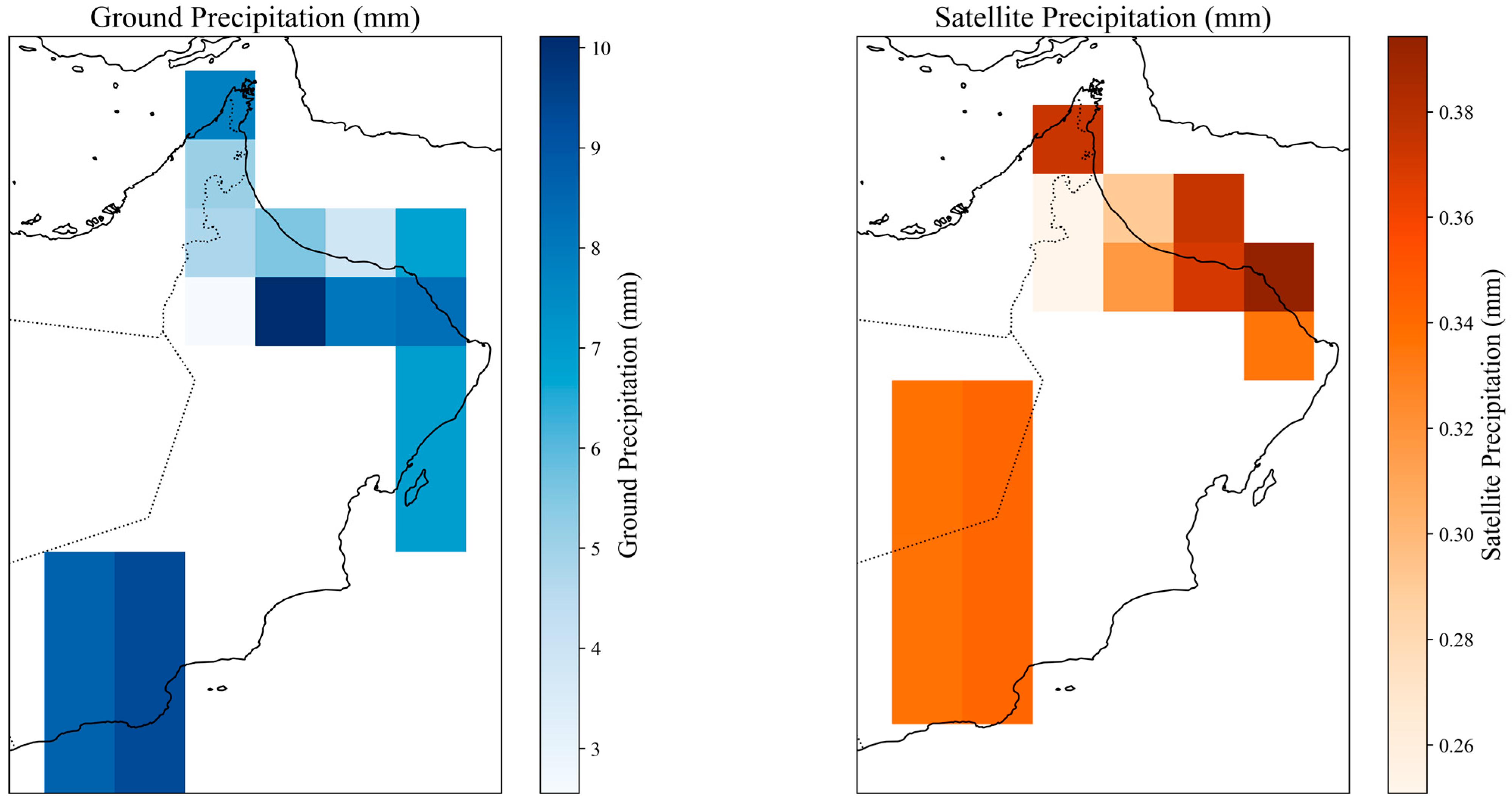
Figure 1. Ground-based vs. satellite-derived precipitation over Oman While both panels show precipitation over the same region, the areas of maximum rainfall do not precisely match, indicating satellite and in situ differences.
Sustainability 17 08321 g001
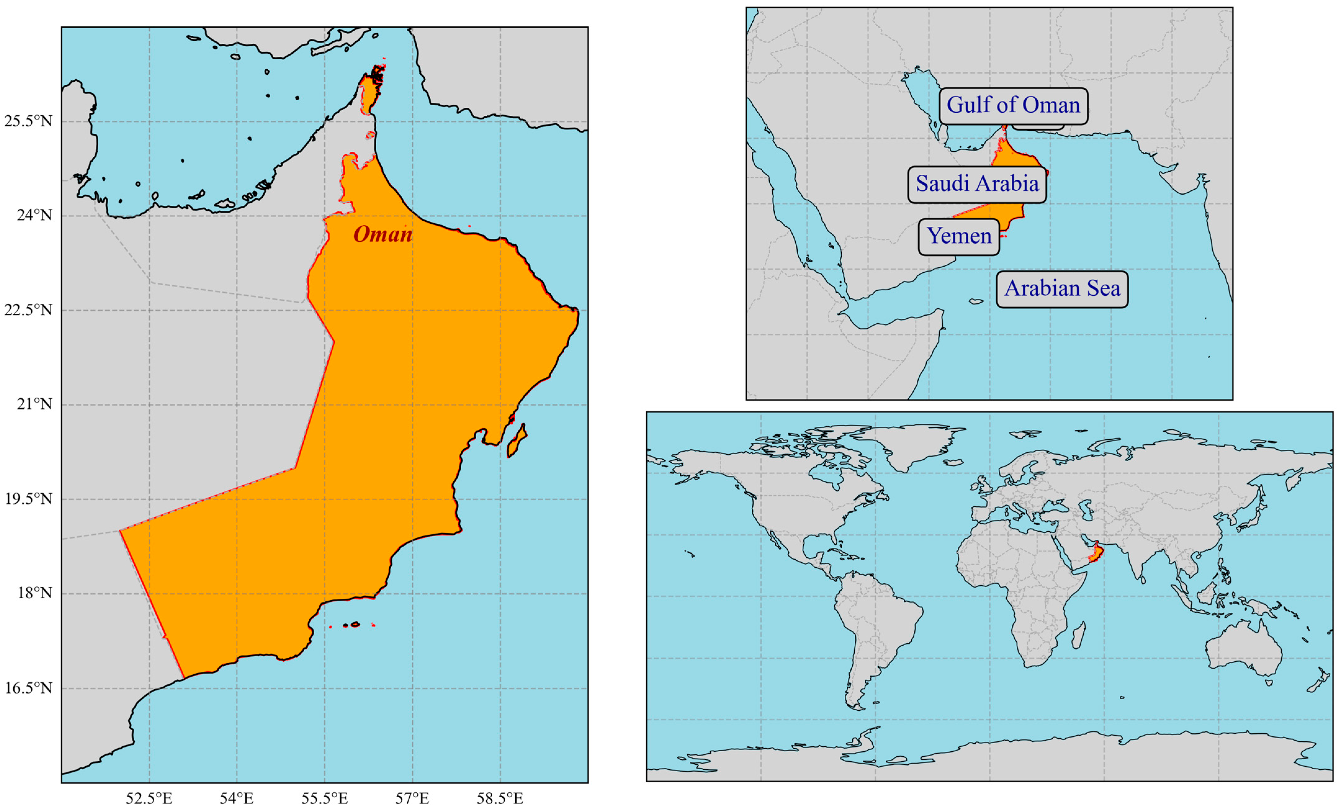
Figure 2. Main map shows Oman and neighbors Top-right inset displays the wider Middle East region. Bottom-right inset highlights Oman’s global location, providing regional and world context.
Sustainability 17 08321 g002
Figure 3. Methodological workflow for evaluating and correcting discrepancies between satellite-based and in situ precipitation data. The process includes data collection, preprocessing, temporal trend analysis, clustering, quantile mapping, model training and evaluation, and trade-off analysis.
Sustainability 17 08321 g003
Figure 4. Quantile–Quantile (Q-Q) plots comparing ground-based and satellite precipitation estimates before (left) and after (right) quantile mapping. For ease of comparison, both plots use the same axis range based on the shared value distribution; however, this does not imply that the two datasets have identical scales. The dashed 1:1 line serves as a reference for perfect agreement.
Sustainability 17 08321 g004
Figure 5. Comparison of precipitation distributions on the most probable range from 0 to 10 mm. The plot overlays ground truth precipitation (red), satellite precipitation before quantile mapping (green), and satellite precipitation after quantile mapping (blue). This plot illustrates that the mapping procedure makes the satellite estimates more in agreement with ground observations for the shared range of precipitation.
Sustainability 17 08321 g005
Figure 6. Spatial distribution of precipitation clusters across Oman. Clusters are concentrated in the northern and southern regions, reflecting the locations of active rain gauge stations and the scarcity of precipitation data in central Oman. Some clusters include spatially dispersed areas grouped based on similar statistical characteristics of the precipitation series.
Sustainability 17 08321 g006
Figure 7. Trade-off Analysis. Solid lines show performance metrics (NSE-blue, KGE-green, RMSE-red, Bias-purple) versus number of clusters. Dashed lines show rate of change (right y-axis).
Sustainability 17 08321 g007
Table 1. Overall Metrics Before and After Quantile Mapping (based on different clusters).
MetricBefore Quantile MappingAfter Quantile Mapping
NSE−0.06570.9825
KGE−0.45450.9910
RMSE25.56173.2741
Bias−0.95650.0011
Table 2. Clustering output.
ClusterNumber of PointsMean LatitudeMean Longitude
015,70622.27003256.776141
124022.06299856.699072
21220.60375756.703053
3121422.46095056.852738
44619.98829755.847929
5117.16024854.220527
648622.40076956.883734
79521.62074956.416030
82820.16514756.076964
9182322.55204256.877945
10123.00132958.878170
11323.28766458.121844
1276822.42452356.902481
1315222.03789356.631199
1436822.08226556.744165
Table 3. The results of the Trade-off analysis.
Number of ClustersNSE Improvement RateKGE Improvement RateRMSE Improvement RateBias Improvement Rate
10.0628210.028291−0.978487−1.699454 × 10⁻⁴
20.0399240.018302−0.730568−1.465856 × 10⁻³
30.0359190.017085−0.833730−1.800803 × 10⁻⁴
40.0119570.006121−0.365616−3.465341 × 10⁻⁴
50.0046210.002058−0.1699832.052146 × 10−4
60.0027080.001339−0.113965−1.036667 × 10⁻⁴
70.0005220.000013−0.0238064.480378 × 10−5
80.0010840.000451−0.052323−1.143269 × 10⁻⁶
90.0008380.000335−0.043902−1.577021 × 10⁻¹⁹
100.0017290.001348−0.106747−2.375115 × 10⁻⁴
110.0004150.000205−0.030815−3.113685 × 10⁻⁶
120.0003280.000162−0.026878−1.171961 × 10⁻⁵
130.0002040.000096−0.0183088.775361 × 10−6
140.0000910.000039−0.0087014.094139 × 10−6
Disclaimer/Publisher’s Note: The statements, opinions and data contained in all publications are solely those of the individual author(s) and contributor(s) and not of MDPI and/or the editor(s). MDPI and/or the editor(s) disclaim responsibility for any injury to people or property resulting from any ideas, methods, instructions or products referred to in the content.