Article

Investigating Spatial Extremes of Annual Daily Precipitation Using CMIP6 Multi-Model Ensembles for Sustainable Flood Risk Assessment

1
School of Climate Change & Adaptation, University of Prince Edward Island, Charlottetown, PE C1A 4P3, Canada
2
School of Mathematical and Computational Sciences, University of Prince Edward Island, Charlottetown, PE C1A 4P3, Canada
3
Faculty of Engineering and Design, Atlantic Technological University, F91 YW50 Sligo, Ireland
*
Author to whom correspondence should be addressed.
Sustainability 2025, 17(18), 8198; https://doi.org/10.3390/su17188198
Submission received: 14 July 2025 / Revised: 12 August 2025 / Accepted: 22 August 2025 / Published: 11 September 2025
(This article belongs to the Section Hazards and Sustainability)

Abstract

This study investigates the spatial characteristics of daily maximum precipitation for Prince Edward Island using a max-stable process model. The ssp126, ssp245, and ssp585 climate change scenarios, indicating low/optimistic, intermediate/in-between, and worst/pessimistic emissions scenarios, respectively, were extracted from 11 global climate model ensembles. For the time periods, the reference (historical) period was from 1971 to 2000, according to the World Meteorological Organization recommendations. Other time periods considered were 2011–2040, 2041–2070, and 2071–2100 as immediate, intermediate, and far future periods, respectively. The spatial trends analysis shows a west-to-east gradient throughout the entire study area. Return levels of 25 years were predicted for all the projections using the spatial generalized extreme value model fitted to the historical period, showing that topography should be included as a covariate in the spatial extreme model. Across the 134 grid points used in the study, the predicted return level for the historical period was 94 mm. Compared with the immediate time period, there is an increase of 47%, 53%, and 50% for the low, intermediate, and worst emission scenarios, respectively. For the intermediate period, there is an increase of 43%, 59%, and 56% for the low, intermediate, and worst emission scenarios, respectively. For the far future period, there is an increase of 49%, 48%, and 84% for the low, intermediate, and worst emission scenarios, respectively. There is a systematic increase in return levels based on the different periods. This shows a high chance of increased risks of extreme events of large magnitudes for this area in the immediate future through to the far future. This study will be useful for engineers, city planners, financial officials, and policymakers tasked with infrastructure development, long-term safety protocols, and sustainability and financial risk management.

1. Introduction

The Paris Agreement aims to limit “the increase in the global average temperature to well below 2 °C above pre-industrial levels” [1]. Furthermore, world leaders have advocated for the “need to limit global warming to 1.5 °C by the end of this century” [1]. Meeting these goals is important; however, efforts must also be made to adapt to the current impacts of continuous increases in global temperatures. Informed decision-making is required to help communities adapt to the effects of climate change, such as heat waves, hurricanes, cyclones, and flooding due to extreme precipitation. Furthermore, hydroclimatic extremes such as excess precipitation are increasing in frequency and intensity, leading to higher flood events; therefore, understanding the spatial variability of these events is crucial for effective flood risk management, sustainability, and climate change adaptation strategies. One method is to have a proactive approach, such as using predictions from climate models. The Coupled Model Intercomparison Project Phase 6 (CMIP6) Multi-Model Ensembles is an effective tool in climate extremes analysis to help researchers and decision-makers compare different climate model predictions up to the year 2100. In addition, using a multi-model ensemble reduces uncertainty when aggregated into a single model, as an input/forcingfor an application of interest. Using multiple CMIP6 scenarios, such as ssp1-2.6 (Shared Socioeconomic Pathway 1 and Radiative Forcing Pathway 2.6 W/m2 by 2100) and ssp3-7.0 (Shared Socioeconomic Pathway 3 and Radiative Forcing Pathway 7.0 W/m2 by 2100) [2,3], is crucial for policy-making bodies and organizations that need information on the impacts of various global emissions pathways. For instance, the Canadian federal and provincial governments are interested in the effects of various emissions scenarios on urban design and development, infrastructure reliability and resilience, disaster preparedness, business risk vulnerability and exposure, etc. This is very important in Atlantic or Maritime Canada, which is exposed to extreme climatic events such as hurricanes. This region is also vulnerable to the impacts of extreme precipitation due to its coastal exposure to erosion, storm surge, and sea level rise. During Hurricane Fiona and Dorian, the reported deaths were 29 and 77, respectively [4,5]. Moreover, the associated damage costs were USD 3.4 billion (Bahamas alone) and USD 600 million (insured damages) for Dorian and Fiona, respectively (IADB, 2019). Therefore, quantifying extreme daily maximum precipitation under a changing climate is crucial.
The CMIP6 dataset has been widely used in extreme climate studies. Huang et al. [6] state that these climate data performed well for consecutive dry days and annual total precipitation but did poorly in reproducing extremely high and low values using 22 GCMs for Central Asia. Zhang et al. [7] used eight extreme precipitation indices to describe the extreme precipitation based on 19 CMIP6 GCMs. From their findings, half of the selected GCMs underestimated extreme precipitation in northern North America and northern Asia. In contrast, there was overestimation in other regions such as the Sahara, Central Asia, and the Arabian Peninsula. Their study concluded that global extreme precipitation will likely increase in cold and polar regions. The authors concluded that the CMIP6 multi-model ensemble performed well in reproducing extreme precipitation in individual ensembles in different climate regions. Kim et al. [8] evaluated the CMIP6 multi-model ensemble for climate extremes. The authors used a generalized extreme value (GEV) technique for the warmest day temperatures, coldest night temperatures, and annual daily maximum precipitation. In their findings, the 20-year return level using CMIP6 for annual daily precipitation shows that dry biases characterize the tropics and subtropics. Other methods to downscale the CMIP6 include the Localized Constructed Analog (LOCA) by [9]. Their study included 27 CMIP6 and 10 members per model with three ssps (i.e., ssp245, ssp370, and ssp585). Their study found that daily precipitation extremes are the longest and largest in the winter (up to 25% for ssp370) in southern Canada and other regions. It is paramount to bias-correct the GCM ensembles before using them for practical applications. Methods include semiparametric quantile mapping [10]. These authors [10] used bias-corrected CMIP6 under four ssps to develop 33-year precipitation levels across the globe. The authors found that this (33-year) return level will increase up to 33.2 mm when compared to the historical period. The authors further confirmed that the 100-year return levels will likely increase to 7.5–21% over the historical level for the worst emission scenario. Moreover, the “100-year historical events will decrease to approximately 50 years and 70 years for the Northern and Southern Hemispheres” [10].
Moreover, Sobie et al. [11] used multivariate techniques to statistically downscale simulations of GCMs for GMIP for 26 models, resulting in the dataset called the “Multivariate Canadian Downscaled Climate Scenarios for CMIP6” (CanDCS-M6). Their approach improved in reproducing the “multivariate and compound climate indices compared to previously used univariate downscaling methods” [11]. The CMIP6 ensemble can also be downscaled to the Statistically Downscaled Indices from Univariate bias-adjusted CMIP6 Simulations (hereafter: CanDCS-U6). CanDCS-U6 has been used to quantify the future streamflow changes in Canada by [12]. Hember et al. [13] also integrated CanDCS-M6 into a modelling application for drought risks to crops. In addition, these indices can also be used in infrastructure planning and future climate extremes [14].
Applying statistical extreme value theory (EVT) effectively captures rare and extreme events since conventional geostatistics are irrelevant as extremes are far from normal. In other words, the approach will include using and extending EVT; therefore, spatial extremes extend the conventional EVT by allowing the marginal parameters to vary spatially. De Haan [15] presented the approach and methodology for spatial extremes of the multivariate extreme value models called the max-stable processes (MSP) [16]. MSP can further be described as having asymptotic motivation, as the univariate generalized extreme value (GEV) distribution can integrate both spatial and temporal dependencies [16]. This means that environmental phenomena such as extreme precipitation causing flooding can be quantified using MSP models with all relevant covariates such as topography, geographical coordinates (i.e., latitude and longitude), temperature, wind speed, and temporal covariates such as time. Takeuchi’s Information Criterion (TIC) is an extension of the Akaike Information Criterion (AIC) designed to address model misspecification. In other words, while AIC assumes models are accurately specified, TIC eased this assumption, and therefore, it is more appropriate in MSP modeling applications such as the spatial extreme characterization of environmental processes. For instance, MSP modeling applications involve heavy-tailed distributions where the real data generating the processes may be outside the available model family [17,18]. MSP models include Smith, Schlather, and Brown–Resnick, extremal-t, etc., which have been used in quantifying the spatial dependency of extreme events globally. The Smith model has been used in capturing the anisotropic dependence using a Gaussian kernel [19]; Davison et al. [20] used the Schlather model in capturing European temperature extremes; Koch et al. [21] used the Brown–Resnick method in modeling precipitation extremes in Germany, while Optiz [22] also used the extremal-t technique in modeling extreme precipitation and wind. Other applications also include [23,24], which focused on extreme precipitation and temperature in the Canadian Prairies. MSP theoretical conceptualizations and applications can be found in studies such as [10,25,26,27].
This study’s primary objective is to quantify the spatial dependency of daily maximum precipitation for PEI in a changing climate. By leveraging the CMIP6 ensembles (CanDCS-U6), this study comprehensively quantifies daily maximum precipitation across diverse climate scenarios to provide a strong understanding of the spatial-temporal trends of extreme precipitation in Prince Edward Island (PEI). Moreover, important metrics such as 25-year return levels for the reference period (1970–2000) were compared with those of the climate emission scenarios (ssp126, ssp245, and ssp585) based on different periods (2011–2040, 2041–2070, and 2071–2100). MSP has been applied in various studies of climatic extremes. Significant gaps exist in applying MSP to characterize the spatial dependency of daily precipitation in PEI. Applying MSP for a regional study allows new insights into extreme precipitation patterns and unique underlying spatial-temporal influences such as geographic coordinates, topography, and climate change. After an exhaustive literature search, this is the first study to quantify PEI’s spatial-temporal trends and 25-year return levels. In other words, this study’s insights will help reassess flood risk preparedness in PEI. Moreover, this study will help in climate change adaptation and resilience in PEI, especially for decision-makers in local and municipal counties and provincial governments in PEI and beyond.

2. Materials and Methods

2.1. Study Area

Prince Edward Island [46.00°–47.08°N, −64.49°–−61.97°W] is the smallest province in Canada and is located in the Gulf of St. Lawrence (Figure 1). The total area is approximately 5000 km2. The province has summer, autumn, winter, and spring temperatures ranging from 20 °C to 34 °C, 8 °C to 22 °C, −3 °C to −11 °C, and 8 °C to 22 °C, respectively [28]. PEI has a coastline approximately 1000 km in length. The province receives an average annual precipitation of 900 to 1200 mm. Snow falls from November until April. The average annual snow depth across the province is approximately 290 cm [28]. As an island in the Atlantic Ocean, PEI is vulnerable to sea level rise, which is estimated at approximately 0.5 to 1 m of erosion loss per year. Moreover, PEI is subjected to storm surges due to storm winds (~15 to 30 km/h) from Atlantic storms and extreme events such as hurricanes. It has been reported that in eastern PEI, between 1970 and 2000, the annual precipitation in the province increased by 6% [29]. During the same period, the annual precipitation in the central and western regions decreased by 5% and 8%, respectively. Being an island surrounded by water, PEI experiences windy conditions. These windy conditions can last for six months with an approximate wind speed of around 25.10 km/h [30]. Figure 1 shows the topography of the study area with an average elevation of 45 m (above sea level). Also, the highest elevation points (~140 m) are the areas of Summerside and Charlottetown. The soil texture is mainly sandstone (red soil) and is rich in iron oxide. Tourism significantly contributes to the province’s revenue and GDP due to the scenic landscapes, beaches, and historic festivals. Due to the lack of rocky subsurface underlay, the province is vulnerable to high soil erosion and degradation. In addition to the low-lying topography of this area, this province is further susceptible to sea-level rise and storm surges. Addressing these challenges requires strategic adaptation planning.

2.2. Multi-Model Ensemble Datasets

This study used the multi-model ensembles developed by Environment Canada (https://climatedata.ca/, accessed on 5 December 2024). The portal hosted two future global climate model simulation phases: Coupled Model Intercomparison Project Phase 5 (CMIP5) and CMIP6. The CMIP6 version is used in this study. CMIP6 uses an ensemble of 26 climate models and has been downscaled to CanDCS-U6, which is a high-resolution statistically downscaled index, and can capture and correctly represent extreme events in Canada. It is based on the Bias Correction/Constructed Analogues with Quantile Mapping reordering (BCCAQv2) and Expert Team on Climate Change Detection and Indices (ETCCDI) techniques, where quantitative indicators such as annual maximum daily temperature, annual minimum temperature, and total daily precipitation can be extracted. The multi-model ensemble used in this study only has 11 climate models, as shown in Table 1. The dataset is from 1950 to 2100, with the historical period ranging from 1950 to 2014. For this study, we followed the World Meteorological Organization (WMO) 30-year intervals, such as 1971–2000, as reference periods. Other periods are divided into 2011–2040, 2041–2070, and 2071–2100, respectively, representing near-future, intermediate-future, and far-future periods. The total daily annual maximum precipitation was extracted from each grid point for all the periods and emission scenarios defined above. The emission scenarios used in this study are based on the ssps framework (ssp126, ssp245, ssp485). They are based on qualitative scenarios that integrate socioeconomic development and quantitative drivers, including GHG emissions, population, and economic growth. The above pathways are further integrated with the RCPs to simulate policy and socioeconomic scenarios. The ssp126, ssp245, and ssp585 are described as follows:
(a)
ssp126: This is a low-emission scenario and is an update of RCP2.6, which assumes a radiative forcing of 2.6 W/m2 by 2100 and represents a sustainable, low-emission pathway that aligns with the Paris Agreement 2 °C target. It is an emission scenario with the narrative of a world that shifts toward sustainability, equity, and international cooperation with CO2 concentrations of around 393 ppm by 2100 [3,31];
(b)
ssp245: This is termed the “middle of the road” scenario, with continuation of the current trajectory with any major shift. It assumes a radiative forcing and estimated warming of 4.5 W/m2 and 2.7 °C, respectively, by 2100. In other words, this emission scenario assumes moderate mitigation efforts, mixed energy sources, a medium population, and economic growth leading to CO2 concentrations of approximately 600 ppm by 2100 [3,31];
(c)
ssp585: This emission scenario assumes little climate policy, high energy demand and resource consumption, and high emission profiles and is also termed “fossil-fueled development–taking the highway”. It assumes emission rise throughout the century, with radiative forcing of 8.5 W/m2 by 2100. The estimated warming is approximately 4.4 °C with a CO2 concentration up to 1135 ppm by 2100, with associated severe impacts [3,31].
Table 1. List of CMIP6 global climate models used in the CanDCS-U6 ensemble.
ModelInstitutionCountry
1CMCC-ESM2Fondazione Centro Euro-Mediterraneo sui Cambiamenti ClimaticiItaly
2GFDL-ESM4NOAA Geophysical Fluid Dynamics LaboratoryUSA
3BCC-CSM2-MRBeijing Climate Centre, China Meteorological AdministrationChina
4INM-CM4-8 Institute for Numerical MathematicsRussia
5FGOALS-g3Institute of Atmospheric Physics, Chinese Academy of SciencesChina
6TaiESM1Research Center for Environmental Changes, Academia SinicaTaiwan
7NorESM2-MMNorwegian Climate CentreNorway
8CanESM5Canadian Centre for Climate Modelling and AnalysisCanada
9KIOST-ESMKorea Institute of Ocean Science and TechnologySouth Korea
10NorESM2-LMNorwegian Climate CentreNorway
11INM-CM5-0Institute for Numerical MathematicsRussia
The above scenarios were selected to qualify a spectrum of socio-economic and climatic futures ranging from optimistic/best (ssp126), in-between (ssp245), and worst/pessimistic (ssp585) situations. The spatial extremes of these scenarios, using daily annual maximum precipitation, were analyzed in this study using the periods defined above.

2.3. Block Maxima and Generalized Extreme Value Theory: A Link to Max-Stable Process for Modeling Spatial Extremes

According to the Fisher–Tippet–Gnedenko Theorem, if we use the block maxima from a dataset (i.e., the yearly maxima of i.i.d. variables (in this case, maximum precipitation), X i ), we can define the block maxima over N observations as M N = m a x X 1 , ,   X N . If a normalizing series exists where a N > 0 and b N , the following applies (refer to Equation (1)):
M N b N a N G x       a s   N
Hence, G(x) is a GEV family, given as Equation (2) [27,32].
G x = e x p 1 + ξ x μ σ 1 ξ ,   ξ   x μ σ > 0
where µ is the location parameter, σ > 0 is the scale parameter, and ξ is the shape parameter that governs the tail of the distribution. In other words, ξ > 0 is heavy-tailed (i.e., Fréchet distribution), ξ = 0 is light-tailed (i.e., Gumbel distribution), and ξ < 0 is short-tailed (i.e., Weibull distribution).
The theoretical formulation of MSP generalizes this GEV to handle spatial applications. MSP models the spatially dependent extreme instead of the independent location. Suppose Z s s ϵ S is a stochastic process domain, S , for any finite set of locations s 1 , , s k . Therefore, the maximum over independent replicates Z s i satisfy the following in Equation (3):
M N s b N s a N s G s x
where G s x is a multivariate or spatially dependent GEV structure, and Z s s ϵ S is termed MSP [20,33]. There are several major MSP models, such as the Smith Model [23], which represents extremes as the maxima of a Poisson point process; the Schlather Model [34], which is based on a spectral construction with a Gaussian random field; the Brown-Resnick Model [35], which is based on the maxima of log-Gaussian processes; and the Extremal-t Model [22], which is based on variation in Schlather’s model using a Student-t process and expressed as Equation (4).
Z s = m a x ξ i . m a x 0 , T i s

2.4. Spatial Dependence Structures of Annual Daily Maximum Precipitation

It is important to check if the daily annual maximum precipitation exhibits spatial dependency to use any of the MSP mentioned above. F-Madogram was introduced by Cooley et al. [36] as the efficient way to assess the extremal dependence function of two spatial locations. The main advantage over conventional variograms in EVT applications is that it is less sensitive to the tail behavior of the distribution. It is also efficient in capturing the spatial dependencies that are specific to particular extreme events. Moreover, tt is a nonparametric measure of dependence, and its connection to the extremal coefficients If Z(s) is an MSP at spatial location s∈Rd, standardized to unit Fréchet margins as follows in Equation (5).
P Z s z = e x p 1 z ,   z > 0
The marginal cumulative distribution function (CDF), F z = exp 1 / z .
Therefore, the F-madogram between two spatial locations, s and s , can be defined as Equation (6).
V F h = 1 2 E F Z s F Z s
where h = { s s } denotes the distance between the two locations [36]. Notably, F-madogram can help in estimating the extremal coefficient, θ h , which lies within the range of 1 and 2. In other words, θ h is an indication of extremal dependencies where θ h = 1 means complete dependencies between spatial locations, while θ h = 2 means independence.
Therefore, F-madogram and extremal coefficient are related through Equation (7).
θ h = 1 + 2 V F h 1 2 V F h

2.5. Takeuchi’s Information Criterion (TIC) in Spatial Extremes

TIC (also known as the Composite Likelihood Information Criterion) is very relevant in MSP modeling due to computational complexity and availability of several competing models. In the presence of the limited identifiability of full likelihoods, composite and pairwise likelohoods are applied. TIC is therefore more efficient than TIC during the model misspecifications.
TIC is defined as shown in Equation (8) [17,37,38].
T I C = 2 l θ ^ + 2 t r J 1 K
where l θ ^ is the maximized (possibly composite) log-likelihood; J is the observed information matrix (negative Hessian of the log-likelihood); and K is the expected outer product of the score vector (the Godambe information matrix when using composite likelihoods). Model selection is performed through the minimization of the TIC defined above; in other words, among several competing models, the model with the least TIC should be selected.
Figure 2 shows the simplified steps followed in this study to characterize the spatial dependencies of extreme precipitation using the CMIP6 ensembles for flood risk assement in PEI.

3. Results and Discussions

3.1. Evaluating the Reliability of GCM Ensembles and Gauge Observations

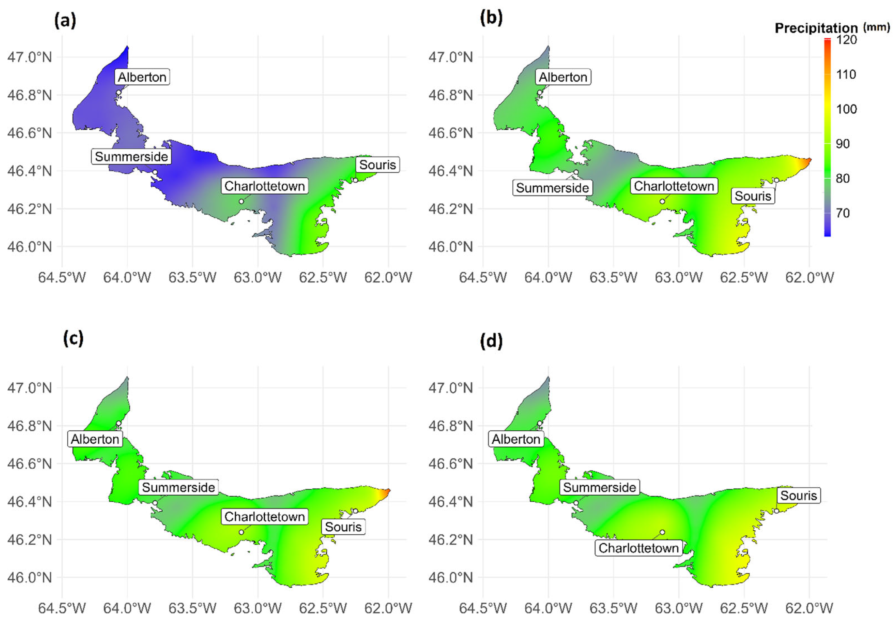
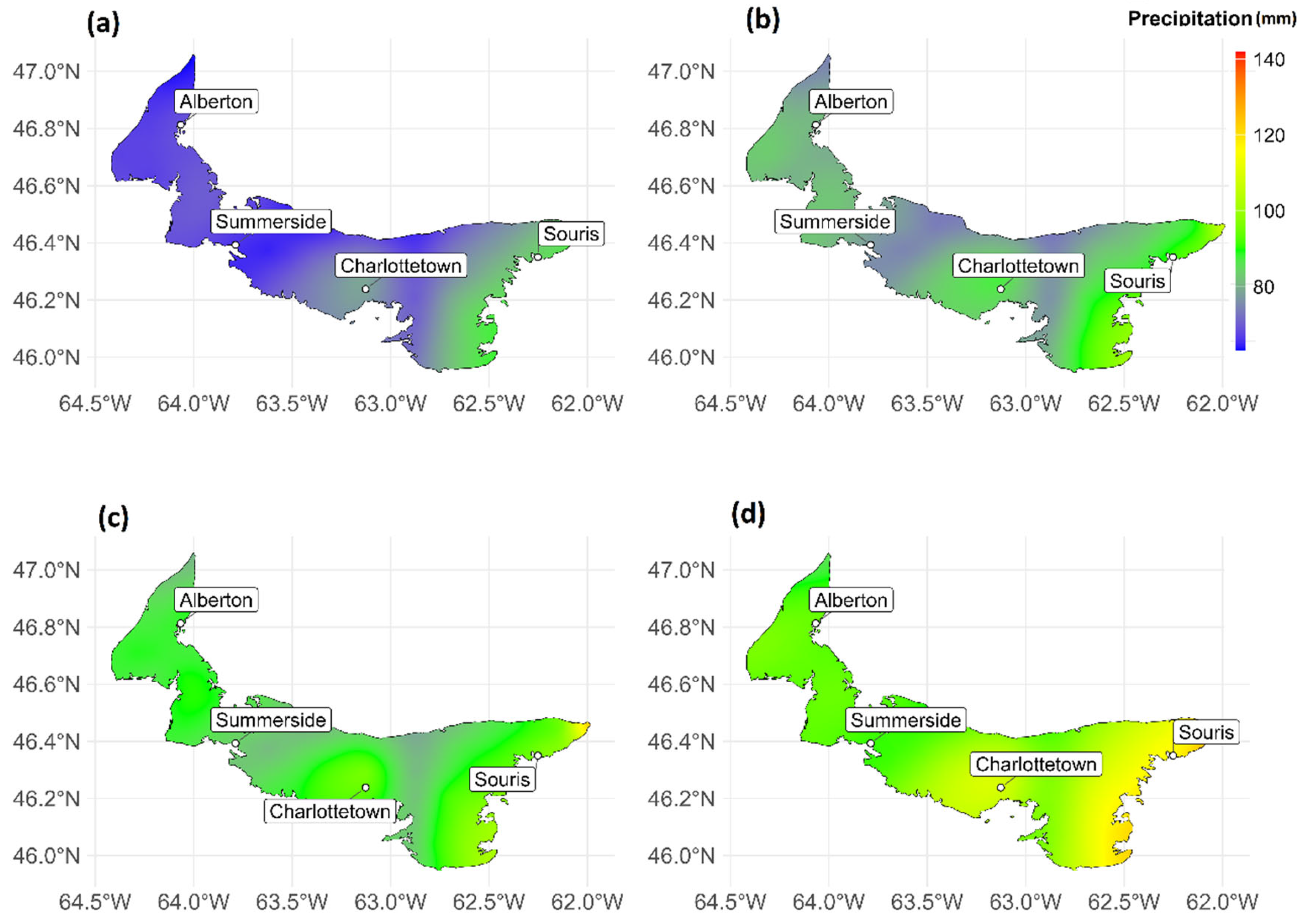
Figure 3, Figure 4 and Figure 5 show plotted annual daily extreme precipitation for the climatic scenarios compared to the observations for 2011–2014, 2041–2070, and 2071–2100, respectively. For the historical period (2011–2014), all the scenarios have values greater than the historical period. Figure 3 shows the historical period with extreme precipitation increased up to 120 mm in the east. There are also west–east gradient patterns in all the scenarios. Similarly, for the period 2041–2070, there is evidence of west–east drift with values up to 120 mm in the eastern portion of the province. Considering the 2071–2100 period, similar patterns are also evident within the province; however, the annual daily precipitation is up to 140 mm. This consistent increase in the climatic projections and scenarios over the historical period shows that an increase in average global temperatures would lead to increased storm energy due to higher sea surface temperatures and more atmospheric instability and chaos. Also, future climatic projections and scenarios from the climate models show the frequency of extreme precipitation days because of global warming. This increase seen in Figure 3, Figure 4 and Figure 5 suggests that increased temperatures will lead to higher evaporation rates from land and oceans, causing more moisture surplus in the atmosphere and leading to heavier and more intense precipitation events supported by the climatic scenarios and projections.

3.2. Spatial-Temporal Trend of Historical and Future Projections of Extreme Precipitation

It is important to explore the possibility of all underlying explanatory variables contributing to extreme precipitation predictions from both temporal and spatial characterization perspectives. Table 2 shows the results of the Multisite Mann–Kendall test for all the climatic scenarios and projections used in this study. There is some evidence of a temporal trend in the ssp456 (in 2041–2070) with a p-value of 0.03, which is less than the 5% significance level. All other scenarios and projections show p-values greater than the 0.05 significance level, meaning there is no evidence of the statistical significance of a temporal trend. This analysis implies that time as a temporal covariate may not be important in the spatial extreme model for all the scenarios, with no statistically significant evidence of a temporal trend. It would be interesting to see the contribution of time as a covariate in spatial extreme model development.
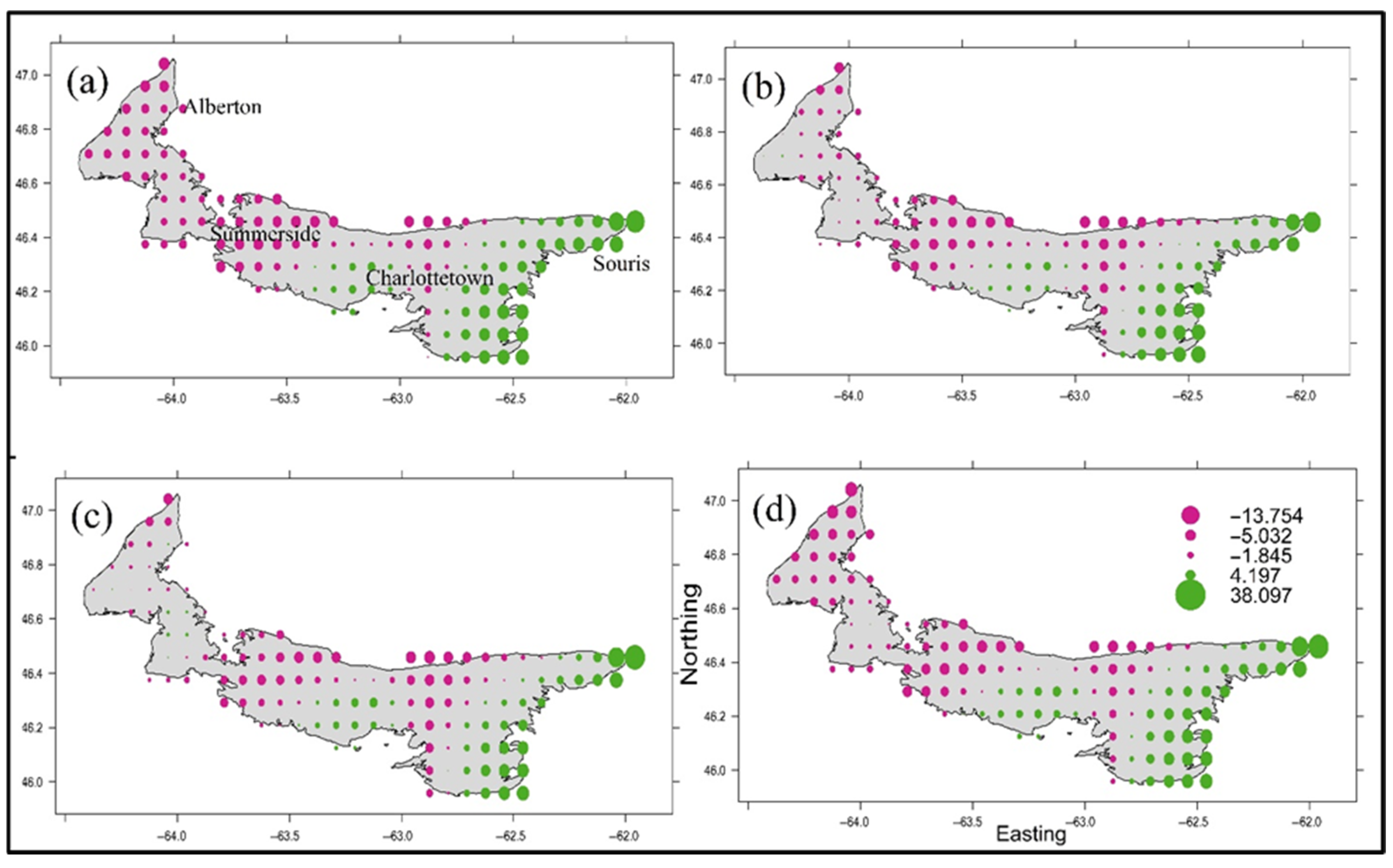
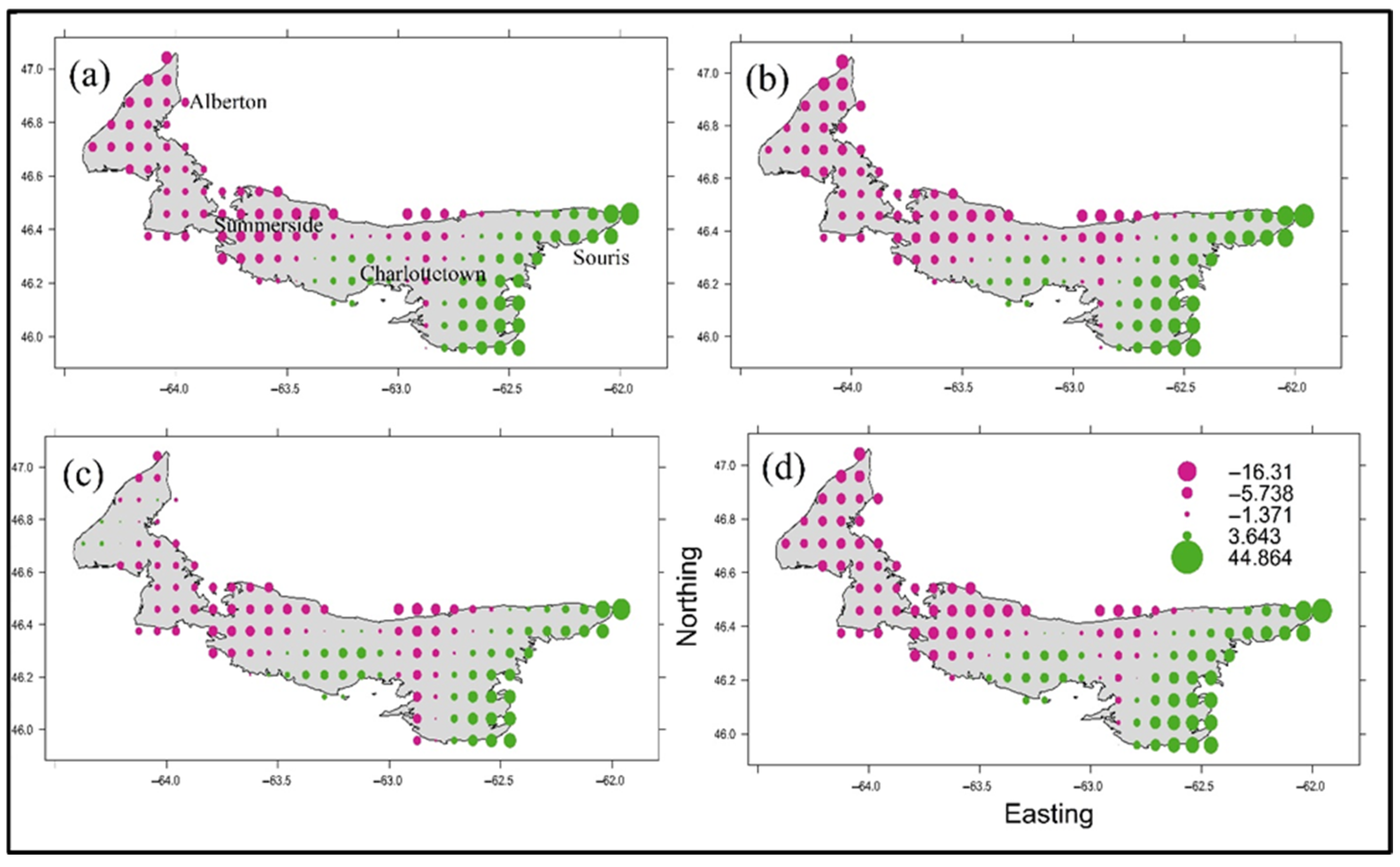
Figure 6, Figure 7 and Figure 8 show the symbol plots of the spatial trends of annual daily maximum precipitation for emission scenarios and future projections. Figure 6 (2011–2040 period) shows that the western and eastern parts of the province show deviation below and above the mean annual maxima daily precipitation, respectively. There is clear evidence of the western–eastern trend as well. The magnitude of deviation below and above the mean annual daily maxima is approximately 13 mm and 30 mm, respectively. This shows that the eastern portion of the province will experience about 38 mm above the mean annual maximum for this projected period. This is crucial, especially for agricultural activities in this part of the province. The above-average annual daily maxima for the eastern section are important for ferry transportation across the Northumberland Strait between Wood Islands, PEI, and Caribou, Nova Scotia. For this future projection, all the emission scenarios show a consistent pattern compared to the reference period. Figure 7 also shows the spatial trend for the 2041–2070 future projections. The western–eastern gradient is also evident with a below–above deviation pattern, respectively. The western–eastern gradient shows deviation below and above the mean annual maxima daily precipitation of approximately 13.7 mm and 38 mm, respectively. The central portion of the study area shows a mixture of deviations above and below the mean annual daily maxima precipitation. This mixture pattern can create uncertainty in the future monitoring of weather patterns for urban cities such as Charlottetown and Summerside. Similarly, Figure 8 follows the same pattern as seen above. The western–eastern gradient shows deviation below and above the mean annual maxima daily precipitation of approximately 14 mm and 35 mm, respectively.
Evidence of this western–eastern drift is an indication of other explanatory variables such as locations (geographical coordinates) and topography. Although not shown, the marginal parameters also show spatial variation from one grid to the other. Therefore, the fitted model should account for this spatial variation in its development.

3.3. Evaluating the Spatial Dependence Structure of Extreme Precipitation

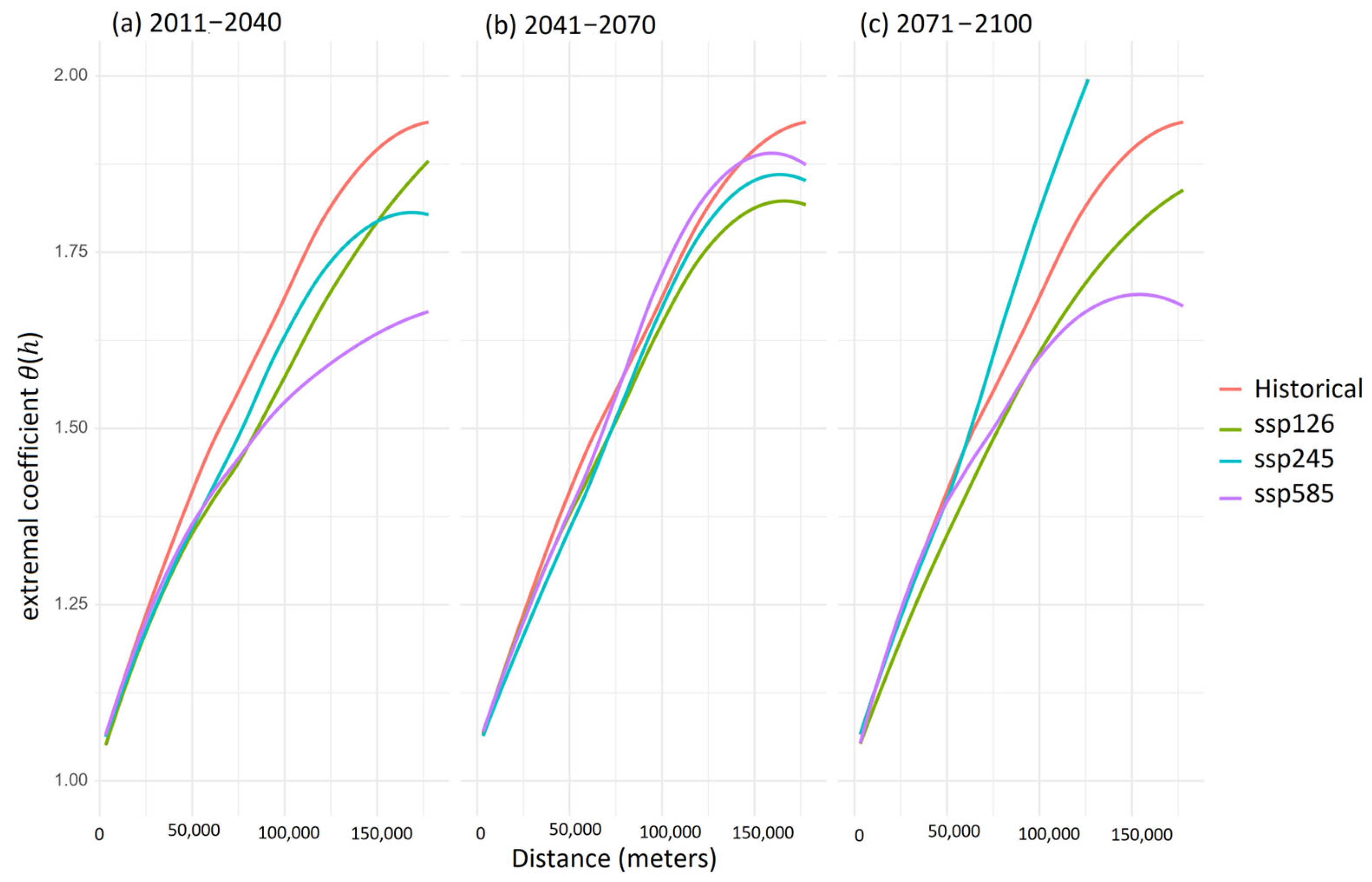
Figure 9 and Figure 10 show the F-madogram and the measure of extremal coefficient, which shows the extremal dependence against distance for the extreme daily annual maximum precipitation historical and all emission scenarios. Figure 9 shows the F-madogram representing the variance in the pairwise maximum annual daily precipitation. It shows a monotonic increase with distance, which shows that at large distances, the spatial dependencies weaken. In small distances, extreme annual daily precipitation at nearby spatial locations is more likely to be similar. For example, periods 2011–2040 and 2041–2070 show a spatial threshold (distance) of around 150,000 m. This indicates the spatial range beyond which extremes in daily annual precipitation can be considered independent. It is interesting to note that for the period 2070–2100 (ssp245), emission scenarios exhibit large V_F (h) compared to other periods. This shows that extreme values at climate grid points are less spatially dependent than in the previous months. This shows that extremes may likely become more localized. In other words, heavy and intensified precipitation may only affect smaller areas rather than an event happening over a large area. PEI’s relatively flat terrain is consistent with the 150,000 m range obtained as the maximum distance at which extreme precipitation recorded from gauging stations or grid points is dependent. The lack of mountain ranges in the region minimizes pockets of localized rainfall patterns due to orographic effects. Nevertheless, in the future, due to rising sea temperature because of global warming, it is expected that there will be more intense precipitation due to enhanced convective activity, leading to more pronounced localized precipitation patterns not seen now (i.e., historical period). Figure 10 also shows the same pattern of all the emission scenarios plateauing at around 150,000 m, except ssp245 in the 2071–2100 period. The wider margin among the scenarios and historical in the 2071–2100 period may be evidence of nonstationary spatial dependence due to climate change. Furthermore, the wider range seen in both the extremal coefficient and F-madogram plots may be due to the increased uncertainty associated with long-range/far future climate projections.

3.4. Spatial Generalized Extreme Value Theorem Model Selection

The best model with the least TIC (TIC = 16,142.93) at the Fréchet scale for the historical period is given in Equation (9).
μ x = 1 + 6.887 × 10 4 l o n x + 2.526 × 10 4 l a t x + 9.925 × 10 5 a l t x σ x = 0.8874997 + 0.0004931 l o n x ξ x = 0.9098
Table 3 gives the SPEV model for all the climatic scenarios and future projections in data space scale. For the location parameter, the intercept values for the model configurations vary between 70 mm and 85 mm. This value represents the baseline level of extremes when the latitude, longitude, and elevation are zero. In other words, it is a theoretical reference point as it sets the starting value for the location parameter. Interestingly, the worst scenario and far future projections have the highest location magnitude of 85 mm. Furthermore, the coefficient for longitude indicates how the baseline level of extremes changes per unit increase in longitude. These coefficients vary between 0.3 and 3.8, suggesting that when longitude increases (moving east), the baseline level of extreme events increases. This is consistent with the impacts of a geographic gradient where eastern areas in PEI experience more intense or frequent extremes (e.g., higher rainfall, stronger winds, or greater temperature extremes) than western areas, as seen in previous sections. Moreover, there is a consistent negative coefficient for the latitude variable, meaning the location parameter decreases as the latitude increases (i.e., moving northward in PEI). In other words, the magnitude of rainfall declines with increasing latitude. This is reflected in all the model configurations except the worst emission scenarios and far future projections. All the elevation coefficients are consistently positive for all the model configurations except the ssp245 (2071–2100). This means that higher elevations experience larger extreme values, which is consistent with phenomena such as the orographic enhancement of precipitation in higher topography
For the scale parameter, the intercept values vary between 16.56 mm and 20.52 mm. This is the value of the scale parameter σ s when all covariates (latitude, longitude, elevation) are zero. It represents the reference variability of extreme values at this reference point. Interestingly, the worst-case emission scenario (ssp585) and far-future projection (2071–2100) have the highest variability at 20.52 mm. This shows the highest variability in this scenario, and the far future projection indicates the long tail of climate inertia, where temperature, sea level, and weather patterns have significantly diverged from the historical period. Considering the longitude coefficients for the model configurations, these are positive, meaning that extreme precipitation variability grows eastward linearly. That is, eastern regions of the province have a wider spread of extremes, leading to an increase in the risk of both high and low outliers of extreme values.
The shape parameters for all the configurations vary between 0.07 and 0.16, which implies that the tail behavior of extremes of all the model configurations across the spatial domain follows a Fréchet distribution with varying degrees of heaviness. The ramifications of this suggest that while the magnitude ( μ ) and variability ( σ ) of extremes may differ spatially due to spatial covariates such as latitude, longitude, topography, and the nature of the extreme; specifically, their potential for rare, very large events remains consistent across the model configurations with the moderate heaviness of the tail of the spatial GEV model.

3.5. Diagnostic Checking of Spatial Extreme Modeling

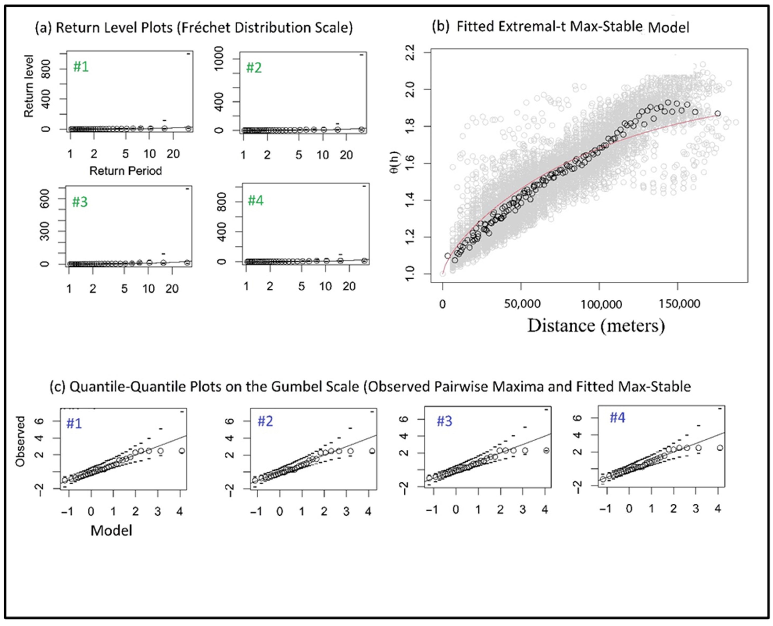
Figure 11 shows the diagnostic plots of the fitted extremal-t model to the extreme precipitation for the historical period. This helps determine if this model fit captures the underlying spatial dependence assumption of the daily maximum precipitation in PEI. As shown in this figure, the spatial dependence structure of the daily maximum precipitation is well captured by the fitted extremal-t model. The extremal-t was used for the scenarios and associated climate projections. The MSP model captured the spatial dependence of annual daily maximum precipitation. The QQ plots (on the Gumbel scale) of the observed pairwise maxima and simulations from the fitted extremal-t Max-Stable model equally show a good fit, as shown in Figure 11. This pattern and performance were also evident in all the scenarios and climate projections.

3.6. Projected Changes in Extreme Precipitation Under Different Scenarios

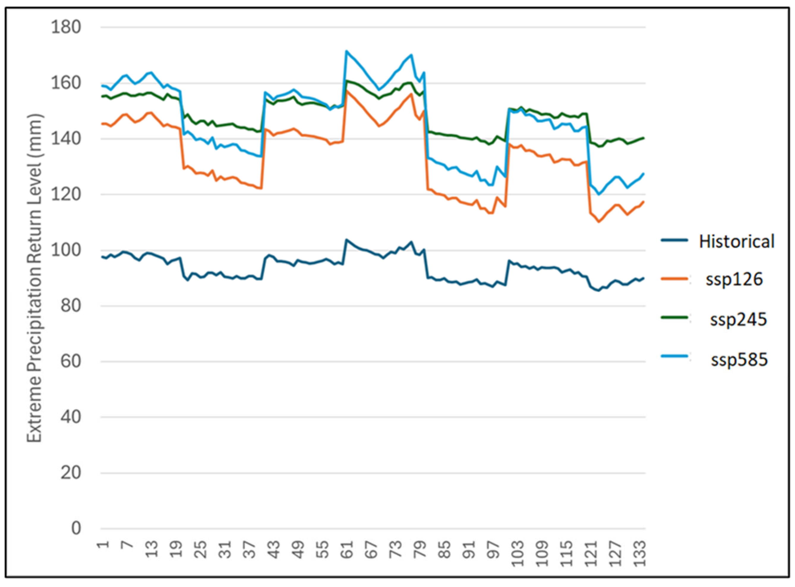
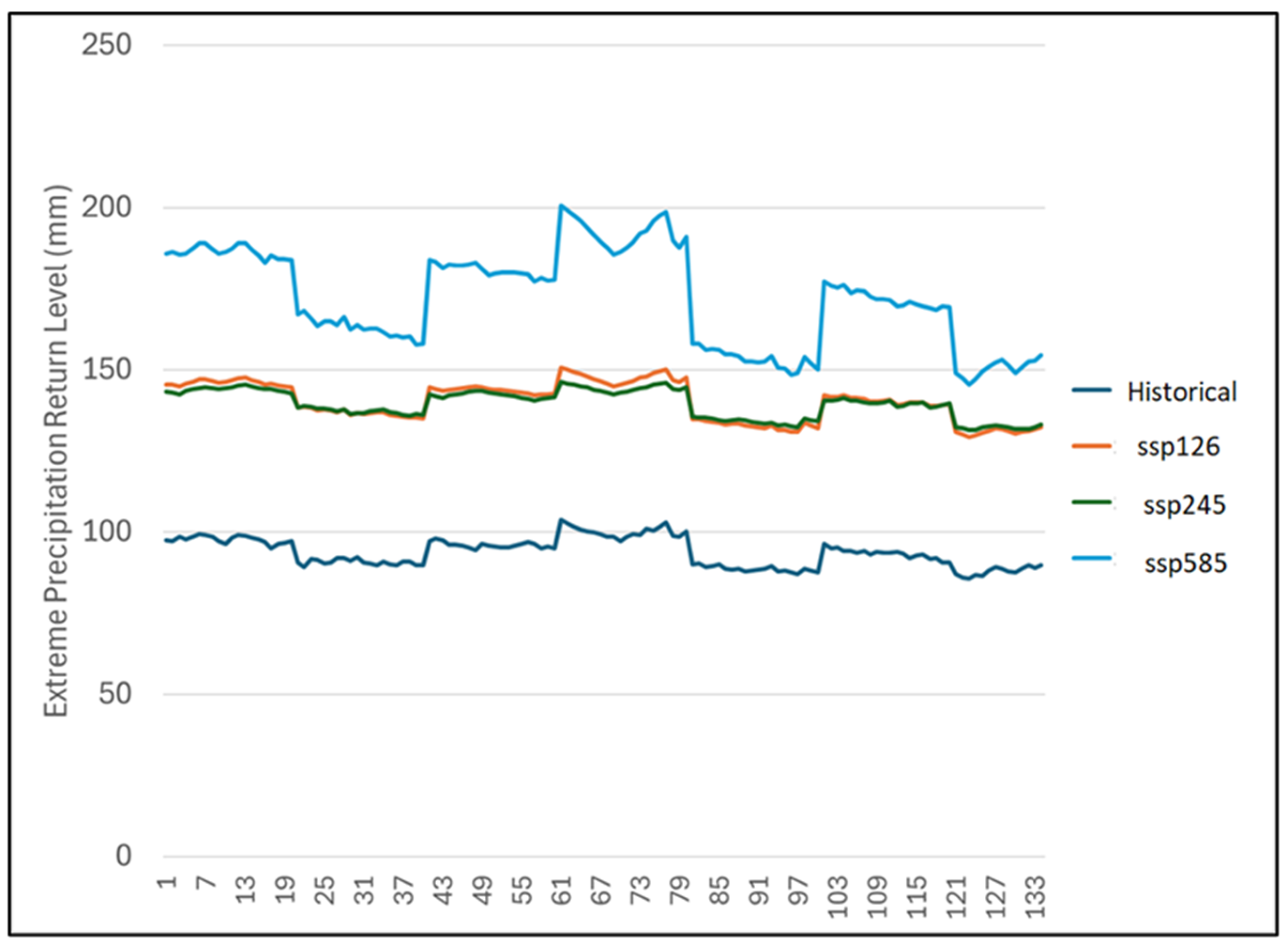
Table 4 shows the qualitative descriptions of spatial predictions for various scenarios and projections. For the 2011–2040 period, the average return levels for the province are 137 mm, 143 mm, and 140.68 mm, for ssp126, ssp245, and ssp585, respectively. The results also show that the maximum return level for ssp126, ssp245, and ssp585 is approximately 152 mm, 157 mm, and 160 mm, respectively. This shows that the percentage increase compared to the historical period is 47%, 53%, and 50%, respectively, for ssp126, ssp245, and ssp585. In the intermediate-future (2041–2070) period, the average predicted return levels for ssp126, ssp245, and ssp585 are around 133mm, 148 mm, and 146 mm, respectively. Moreover, the maximum return levels for ssp126, ssp245, and ssp585 are 157 mm, 160 mm, and 171 mm, respectively. This indicates a percentage increase of 43%, 59%, and 56% for ssp126, ssp254 and ssp585, respectively. Furthermore, for the 2071–2100 projection, the predicted average return level for ssp126, ssp245, and ssp585 is approximately 140 mm, 139 mm, and 172 mm, respectively. The percentage increase compared to the historical period is 49%, 48%, and 84% for ssp126, ssp245, and ssp585, respectively. The maximum return level for this period is approximately 150 mm, 146 mm, and 200 mm for the ssp126, ssp245, and ssp585 emissions scenarios, respectively. All the above quantitative results show a substantial increase in the intensity of daily maximum precipitation for all scenarios and projections. In other words, even in the low-emission scenarios (ssp126), the “sustainable development” pathway, where it assumes that there would be significant global agreement and common ground on climate initiatives, there is substantial risk related to the intensification of extreme precipitation. Moreover, the “middle of the road” and “fossil fuel economy” scenarios also substantially increase the intensity of extreme precipitation.
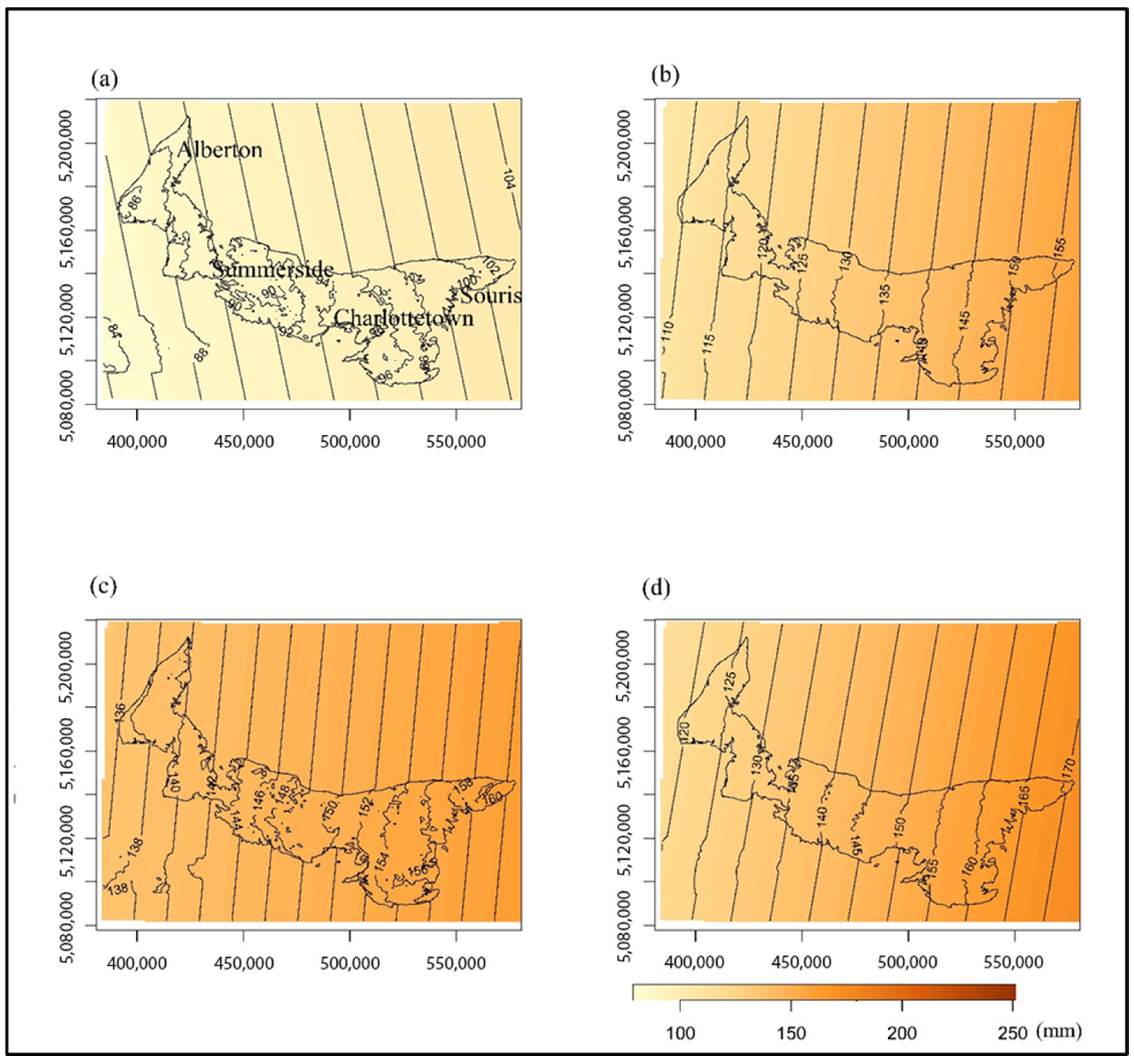
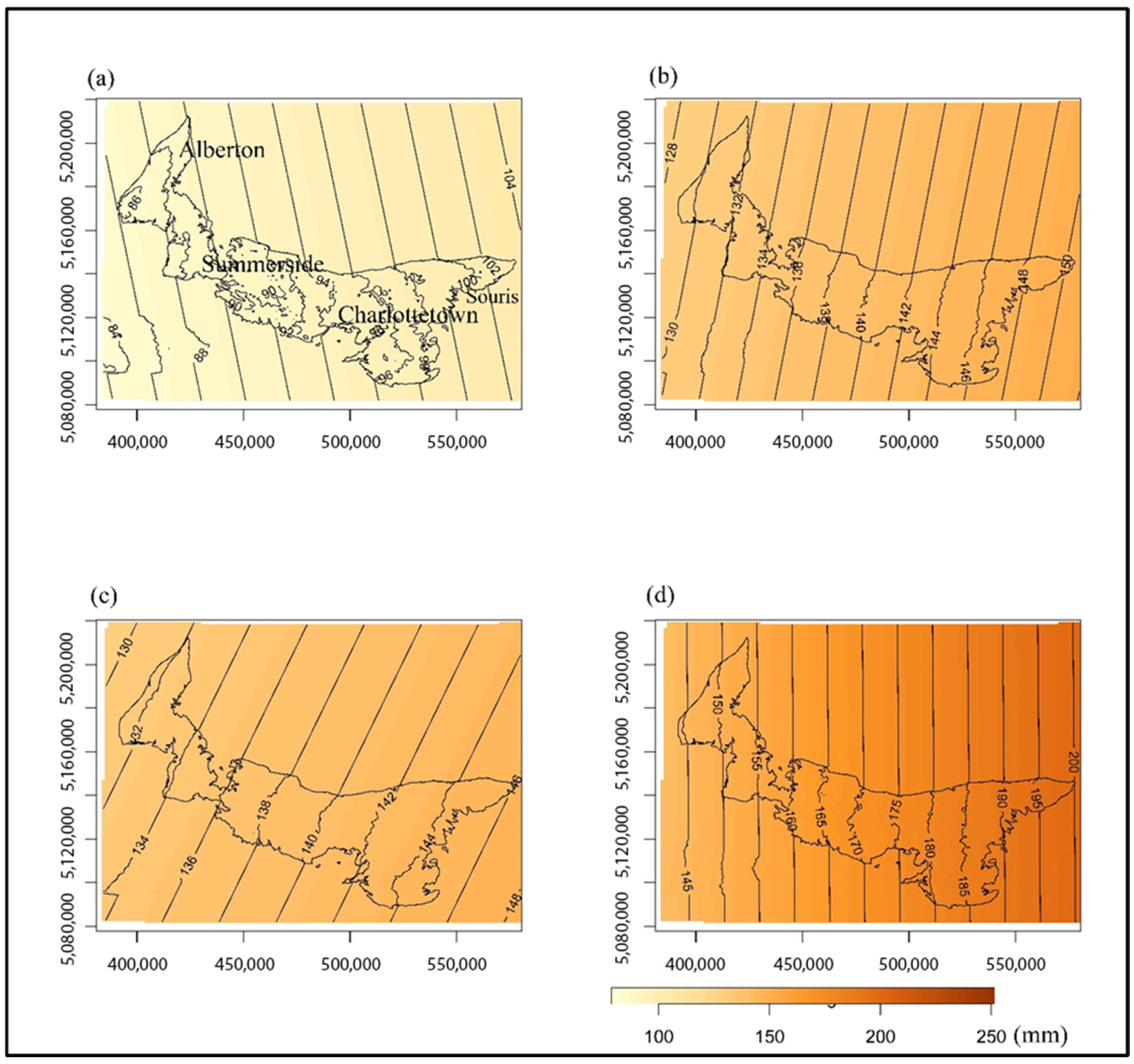
Figure 12, Figure 13 and Figure 14 show the spatial distribution and highlight the key differences in the predicted 25-year return levels of the daily maximum precipitation of PEI for reference and future projections. The contour lines show the systematic increase in the return levels across the emissions scenarios. For the 2011–2040 period (Figure 12), the western–eastern gradient in Figure 2 is correctly reproduced. The return levels around A (Alberton), S (Summerside), C (Charlottetown), and SR (Souris) are 90 mm, 90 mm, 94 mm, and 100 mm, respectively, for the historic period. For ssp126, this increased to 126 mm, 136 mm, 140 mm, and 150 mm, respectively. Similarly, the return level increased to 135 mm, 136 mm, 148 mm, and 164 mm for A, S, C, and SR, respectively. For all the scenarios, there is an increase in the return level values over the historical period. Considering the intermediate future projection (2041–2070) as shown in Figure 13, ssp126 indicates approximately 116 mm, 120 mm, 135 mm, and 155 mm for Alberton, Summerside, Charlottetown, and Souris, respectively. For ssp245, the contour line for this period’s return level is 140 mm, 144 mm, 154 mm, and 160 mm, respectively. For ssp585, it has a return level of 129 mm, 132 mm, 150 mm, and 170 mm for Alberton, Summerside, Charlottetown, and Souris, respectively. This period also consistently increased in the 2011–2040 climatic projection. For the far future projections in Figure 14, ssp126 indicates that Alberton, Summerside, Charlottetown, and Souris would have a return level of approximately 132 mm, 134 mm, 140 mm, and 150 mm, respectively. Furthermore, for ssp245, the return levels for Alberton, Summerside, Charlottetown, and Souris are approximately 133m, 134 mm, 140 mm, and 146 mm, respectively. Finally, ssp585 has a return level of 154 mm, 156 mm, 170 mm, and 200 mm, respectively. This is a significant increase compared to other emission scenarios. This shows that this worst-case scenario, due to increased average global temperatures causing climate change, would significantly increase the return level of extreme daily precipitation.

3.7. Variability of Return Levels for Historical and Future Projections of Extreme Precipitation

Furthermore, we explored the consistency in return level variability using the 134 grid points that cover the study area (Figure 15, Figure 16 and Figure 17). The results show a sustained increase for all the scenarios and future projections for all the grid points. Figure 15 highlights the key differences between the emission scenarios for the period 2011–2040. There is evidence of an increase in intensity and consistency in spatial patterns across the grid points. It is also interesting to note the closeness in the return levels for all the emission scenarios across the grid points. Figure 16 also shows the spatial pattern of the predicted return level for the 2041–2070 period. The consistency in the return level variability can be seen across the grid points; however, there are disparities in the values of the emission scenarios. Figure 17 shows large differences between the worst and other emission scenarios for the 2071–2100 period. This shows that the impacts of the worst emission scenarios for the end of the 21st century will be catastrophic from an extreme precipitation intensity perspective. The downtrend seen in all three plots replicates the west–east extreme precipitation gradients discussed above. Moreover, the wider margin seen in Figure 17 may be due to the uncertainty inherent in longer far-future climate projections.

3.8. Implications of Spatial Extremes in Prince Edward Island

There are socio-economic implications of the historical and climatic projected spatial patterns of extreme precipitation in terms of regional climate risk for PEI. These include flood risk management, urban planning, design and development, the development of new building codes, and the resilience of old infrastructure such as bridges, roads, and buildings. Extreme rainfall would impact agricultural activities, causing erosion, waterlogging, and the leaching of nutrients into the groundwater or open freshwater. Waterlogged farmlands can delay farm operations, causing farmers to miss important farming dates, reducing yield quantity and quality. Excessive moisture due to extreme rainfall can also trigger pest and disease infestations. From a public health management standpoint, extreme rainfall with high intensity can also lead to contaminated overland flow (runoff), which can cause drinking water pollution and amplify the risk of waterborne diseases and epidemics. Another major implication of this study is the possibility of higher insurance costs, especially for houses and properties now in the range of the extreme precipitation spatial extent. In other words, extreme precipitation could lead to business disruptions in all industries, particularly for fisheries and construction. From the beginning, this study has shown there is a need for various adaptation strategies ranging from community-based, land planning, climate finance, and green infrastructure (e.g., urban restoration of wetlands) to counter the significant increase in the intensity of extreme precipitation using various emissions scenarios and future projections when compared to the historical period as demonstrated in this study.
For future recommendations and work, it would be interesting to assess the interactions between precipitation extremes and other important climatic variables such as temperature and snowpack. Furthermore, it would be interesting to quantify the uncertainty in the multi-model ensembles using models other than the 11 used in this study. Moreover, other advanced machine-learning-based downscaling techniques could also be used in the regional climate model datasets. Environment Canada has a newly downscaled version of CMIP6, which uses a multivariate downscaling method that will use an ensemble of the same climate models as CanDCS-U6, referred to as CanDCS-M6 or M6; it would be interesting to see the improvement in these new data on the current study. Evaluating the impacts of urbanization or land use change on the extreme precipitation pattern of the province under a changing climate is another interesting future research prospect. This new dataset (not used in this study) also produced ssp370, which sits between ssp245 and ssp585. Future research should include this emission scenario and its impacts on climatic extremes in the North Atlantic.

4. Conclusions

This study applied the spatial extremal technique to quantify the spatial extreme and dependency of daily maximum precipitation in PEI using CMIP6 multi-model ensembles. The study provides insights into the impacts of climate change due to extreme daily precipitation and the spatial heterogeneity across the province. Return levels were predicted for the reference period (1971–2000) and future periods (2011–2040, 2041–2070, and 2071–2100) under low, intermediate, and worst emission scenarios. This study could serve as a methodological blueprint for other regions in PEI and beyond on applying MSP in multi-model ensembles of spatial extremes. This study demonstrated advanced statistical methods incorporating important covariates in regional spatial extremes of daily maximum precipitation. The study provides an important direction for a precise study that applies to climatic resilience, disaster preparedness, and urban design and development
The following are the conclusions drawn from this study:
(a)
The spatial trend of extreme daily precipitation shows a west–eastern gradient for the historical and future periods. Also, the temporal trend using the multivariate (Multisite) Mann–Kendall Test indicates there was no statistically significant trend in both historical and future periods;
(b)
The fitted extremal-t max-stable model correctly captured the spatial dependency and characteristics of extreme daily precipitation for the reference period and future projections. The predicted return levels are within the 95% confidence levels of the predicted results, meaning that this fitted model can be used to model both historical and future extremes in PEI;
(c)
Considering the 25-year return levels extracted from the 134 grid points of the multi-model ensembles, the average return level was 94 mm across PEI for the historical period. For the 2011–2040, 2040–2070, and 2070–2100 periods, there is an increase in the return levels up to 50%, 56%, and 84%, respectively. This shows there would be systematic increases in the intensity of extreme precipitation in the future under all emission scenarios.
This study provides evidence of the necessity of integrating spatial characteristics of extremes in climate projections to quantify infrastructure design and sustainable development risks and ensure decisions are being made based on facts and quantitative evidence. Moreover, with a high likelihood of the increased frequency and magnitude of extreme precipitation events in PEI, this study contributes to the research literature in the Maritime provinces of Canada and beyond, especially in addressing climate change impacts and adaptation strategies for flood risk management.

Author Contributions

Conceptualization: A.B.; methodology: A.B. and P.S.; formal analysis and investigation: A.B. and P.S.; writing—original draft preparation: A.B. and P.S.; writing—review and editing: A.B., P.S. and U.R.; contribution to the final manuscript: A.B., P.S. and U.R. All authors have read and agreed to the published version of the manuscript.

Funding

This research received no external funding.

Institutional Review Board Statement

Not applicable.

Informed Consent Statement

Not applicable.

Data Availability Statement

Climate Model Datasets used are publicly available at https://climatedata.ca/download/ (accessed on 1 October 2024).

Conflicts of Interest

The authors declare no known competing financial interests or personal relationships that could have appeared to influence the work reported in this paper.

References

  1. United Nations Framework Convention on Climate Change. The Paris Agreement. 2024. Available online: https://unfccc.int/process-and-meetings/the-paris-agreement/the-paris-agreement (accessed on 5 December 2024).
  2. O’Neill, B.C.; Kriegler, E.; Riahi, K.; Ebi, K.L.; Hallegatte, S.; Carter, T.R.; Mathur, R.; van Vuuren, D.P. A new scenario framework for climate change research: The concept of shared socioeconomic pathways. Clim. Change 2014, 122, 387–400. [Google Scholar] [CrossRef]
  3. IPCC. Climate Change 2021: The Physical Science Basis. Contribution of Working Group I to the Sixth Assessment Report of the Intergovernmental Panel on Climate Change; Cambridge University Press: Cambridge, UK, 2021; Available online: https://www.ipcc.ch/report/ar6/wg1/ (accessed on 5 December 2024).
  4. Inter-American Development Bank. Assessment of the Effects and Impacts of Hurricane Dorian in the Bahamas; Inter-American Development Bank: Washington, DC, USA, 2019; Available online: https://www.iadb.org/en/news/damages-and-other-impacts-bahamas-hurricane-dorian-estimated-34-billion-report (accessed on 5 December 2024).
  5. Insurance Bureau of Canada. Hurricane Fiona Causes $660 Million in Insured Damage. 19 October 2022. Available online: https://www.ibc.ca/news-insights/news/hurricane-fiona-causes-660-million-in-insured-damage (accessed on 5 December 2024).
  6. Huang, X.; Wang, Y.; Ma, X. Simulation of extreme precipitation changes in Central Asia using CMIP6 under different climate scenarios. Theor. Appl. Climatol. 2024, 155, 3203–3219. [Google Scholar] [CrossRef]
  7. Zhang, B.; Song, S.; Wang, H.; Duan, Y.; Liu, J.; Tang, G. Evaluation of the performance of CMIP6 models in simulating extreme precipitation and its projected changes in global climate regions. Nat. Hazards 2024, 121, 1737–1763. [Google Scholar] [CrossRef]
  8. Kim, Y.-H.; Min, S.-K.; Zhang, X.; Sillmann, J.; Sandstad, M. Evaluation of the CMIP6 multi-model ensemble for climate extreme indices. Weather Clim. Extrem. 2020, 29, 100269. [Google Scholar] [CrossRef]
  9. Pierce, D.W.; Cayan, D.R.; Feldman, D.R.; Risser, M.D. Future increases in North American extreme precipitation in CMIP6 downscaled with LOCA. J. Hydrometeorol. 2023, 24, 951–965. [Google Scholar] [CrossRef]
  10. Abdelmoaty, H.M.; Papalexiou, S.M. Change of extreme precipitation in CMIP6 projections: Should we use stationary or nonstationary models? J. Clim. 2023, 36, 2999–3014. [Google Scholar] [CrossRef]
  11. Sobie, S.R.; Ouali, D.; Curry, C.L.; Zwiers, F.W. Multivariate Canadian downscaled climate scenarios for CMIP6 (CanDCS-M6). Geosci. Data J. 2024, 11, 806–824. [Google Scholar] [CrossRef]
  12. Mousavi, R.; Johnson, D.L.; Byrne, J.M.; Kroebel, R. Projected 21st Century Drought Condition in the South Saskatchewan River Watershed: A Case Study in the Canadian Prairies. Atmosphere 2024, 15, 1292. [Google Scholar] [CrossRef]
  13. Hember, R.A.; Werner, A.T.; Huang, J. Projecting future drought risk for Canadian agriculture using downscaled CMIP6 climate data. Agric. For. Meteorol. 2023, 321, 109091. [Google Scholar] [CrossRef]
  14. Bonsal, B.R.; Cannon, A.J.; Anslow, F.S. Projected changes to climate extremes over Canada using downscaled CMIP6 scenarios. Clim. Change 2022, 172, 23. [Google Scholar]
  15. de Haan, L. A spectral representation for max-stable processes. Ann. Probab. 1984, 12, 1194–1204. [Google Scholar] [CrossRef]
  16. Padoan, S.A.; Ribatet, M.; Sisson, S.A. Likelihood-based inference for max-stable processes. J. Am. Stat. Assoc. 2010, 105, 263–277. [Google Scholar] [CrossRef]
  17. Takeuchi, K. Distribution of information statistics and the criteria for adequacy of models. Math. Sci. 1976, 153, 12–18. [Google Scholar]
  18. Konishi, S.; Kitagawa, G. Information Criteria and Statistical Modeling; Springer: Berlin/Heidelberg, Germany, 2008. [Google Scholar] [CrossRef]
  19. Blanchet, J.; Davison, A.C. Spatial modeling of extreme snow depth. Ann. Appl. Stat. 2011, 5, 1699–1725. [Google Scholar] [CrossRef]
  20. Davison, A.C.; Padoan, S.A.; Ribatet, M. Statistical modeling of spatial extremes. Stat. Sci. 2012, 27, 161–186. [Google Scholar] [CrossRef]
  21. Koch, T.; Naveau, P.; Ribatet, M. Spatial extremes: Modeling rainfall in France. J. De La Société Française De Stat. 2013, 154, 128–144. [Google Scholar]
  22. Opitz, T. Extremal-t processes: Elliptical domain of attraction and a spectral representation. J. Multivar. Anal. 2013, 122, 409–413. [Google Scholar]
  23. Boluwade, A. Stochastic modeling of spatial dependency structures of extreme precipitation in the Northern Great Plains using max-stable processes. J. Water Clim. Change 2024, 14, 3131–3149. [Google Scholar] [CrossRef]
  24. Boluwade, A.; Sheridan, A.P.; Farooque, A.A. Spatial modeling of extreme temperature in the Canadian Prairies using max-stable processes. Results Eng. 2024, 21, 101879. [Google Scholar] [CrossRef]
  25. de Haan, L.; Pereira, T.T. Spatial extremes: Models for the stationary case. Ann. Stat. 2006, 34, 146–168. [Google Scholar] [CrossRef]
  26. Coles, S.G.; Tawn, J.A. Modelling extremes of the areal rainfall process. J. R. Stat. Soc. Ser. B 1996, 58, 329–347. [Google Scholar] [CrossRef]
  27. Ribatet, M. Modelling spatial extremes using max-stable processes. In Nonlinear and Stochastic Climate Dynamics; Hannachi, A., Battisti, D.S., Schultz, D.M., Eds.; Cambridge University Press: Cambridge, UK, 2017; pp. 369–391. [Google Scholar] [CrossRef]
  28. Government of Prince Edward Island. PEI Climate and Weather. 2022. Available online: https://www.princeedwardisland.ca/en/information/environment-energy-and-climate-action/pei-climate-and-weather (accessed on 5 December 2024).
  29. Bhatti, A.; Farooque, A.; Krouglicof, N.; Peters, W.; Acharya, B.; Li, Q.; Ahsan, M.S. Climate change impacts on precipitation and temperature in Prince Edward Island, Canada. World Water Policy 2021, 7, e12046. [Google Scholar] [CrossRef]
  30. Weather Spark. Average Weather in Charlottetown, Prince Edward Island, Canada Year Round. 2025. Available online: https://weatherspark.com/y/28438/Average-Weather-in-Charlottetown-Prince-Edward-Island-Canada-Year-Round (accessed on 5 December 2024).
  31. Meinshausen, M.; Nicholls, Z.R.J.; Lewis, J.; Gidden, M.J.; Vogel, E.; Freund, M.; Beyerle, U.; Menne, B. The shared socio-economic pathway (SSPSSP) greenhouse gas concentrations and their extensions to 2500. Geosci. Model Dev. 2020, 13, 3571–3605. [Google Scholar] [CrossRef]
  32. Coles, S. An Introduction to Statistical Modeling of Extreme Values; Springer: Berlin/Heidelberg, Germany, 2001. [Google Scholar]
  33. de Haan, L.; Ferreira, A. Extreme Value Theory: An Introduction; Springer: Berlin/Heidelberg, Germany, 2006. [Google Scholar]
  34. Schlather, M. Models for stationary max-stable random fields. Extremes 2002, 5, 33–44. [Google Scholar] [CrossRef]
  35. Brown, B.M.; Resnick, S.I. Extreme values of independent stochastic processes. J. Appl. Probab. 1977, 14, 732–739. [Google Scholar] [CrossRef]
  36. Cooley, D.; Naveau, P.; Poncet, P. Variograms for spatial max-stable random fields. In Dependence in Probability and Statistics; Bertail, P., Soulier, P., Doukhan, P., Eds.; Springer: Berlin/Heidelberg, Germany, 2006; Volume 187, pp. 373–390. [Google Scholar]
  37. Akaike, H. Information theory and an extension of the maximum likelihood principle. In Second International Symposium on Information Theory; Petrov, B.N., Csáki, F., Eds.; Akadémiai Kiadó: Budapest, Hungary, 1973; pp. 267–281. [Google Scholar]
  38. Varin, C.; Vidoni, P. A note on composite likelihood inference and model selection. Biometrika 2005, 92, 519–528. [Google Scholar] [CrossRef]
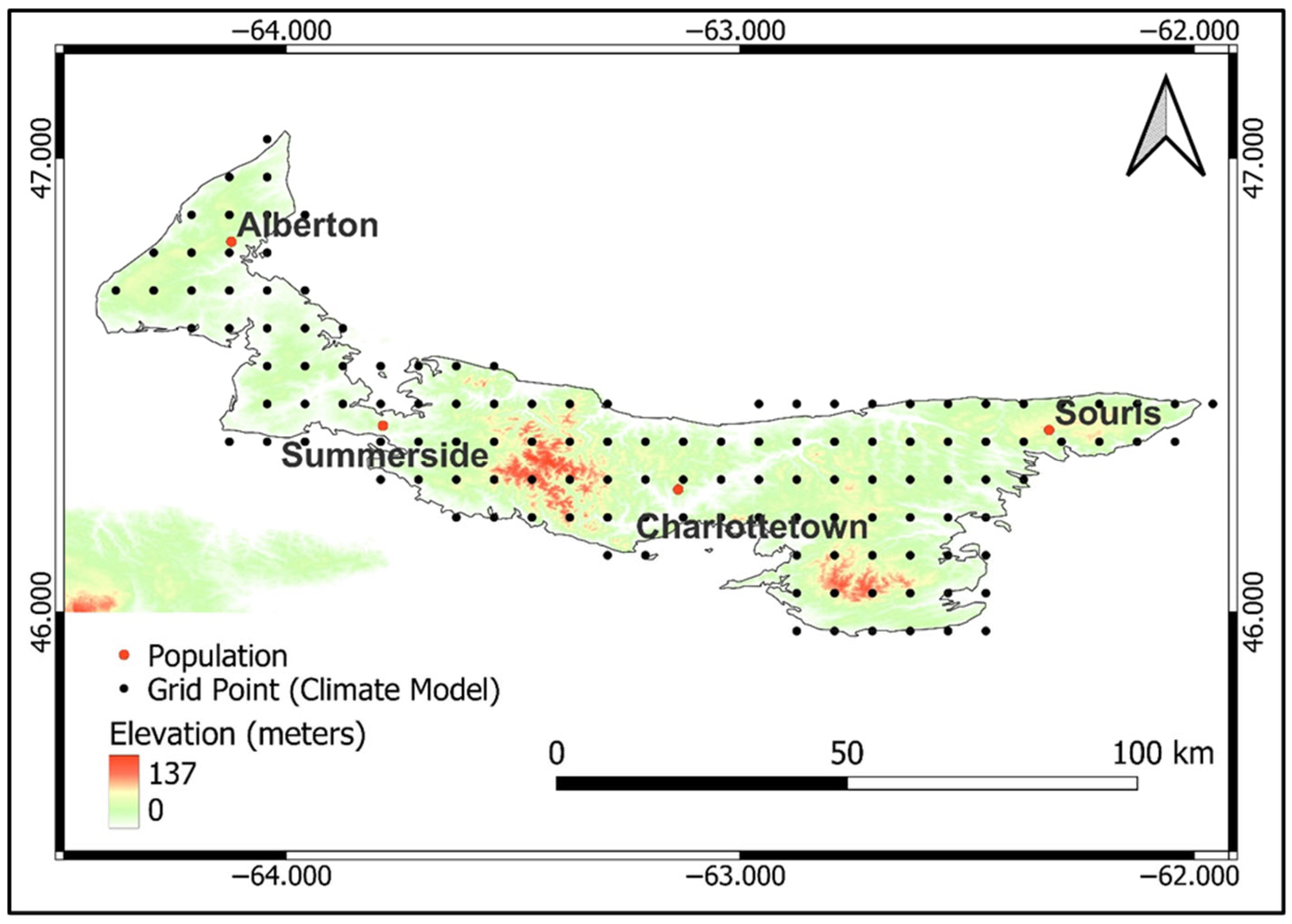
Figure 1. Elevation map of Prince Edward Island showing the topography and locations of CMIP6 grid points used in the study.
Sustainability 17 08198 g001
Figure 2. Flow chart of spatial extreme model development, prediction, and simulation for daily maximum precipitation in Prince Edward Island.
Sustainability 17 08198 g002
Figure 3. Spatial distribution of the average daily maximum precipitation for (a) a historical period, (b) low emissions (ssp126), (c) intermediate emissions (ssp245), and (d) high emissions (ssp4585) for Prince Edward Island from the CMIP6 Multi-Model Estimate for 2011–2041 for a climatic emission scenario.
Sustainability 17 08198 g003
Figure 4. Spatial distribution of the average daily maximum precipitation for (a) a historical period, (b) low emissions (ssp126), (c) intermediate emissions (ssp245), and (d) high emissions (ssp4585) for Prince Edward Island from the CMIP6 Multi-Model Estimate for 2041–2071 for a climatic emission scenario.
Sustainability 17 08198 g004
Figure 5. Spatial distribution of the average daily maximum precipitation for the (a) historical period, (b) low emissions (ssp126), (c) intermediate emissions (ssp245), and (d) high emissions (ssp4585) for Prince Edward Island from the CMIP6 Multi-Model Estimate for 2071–2100 for a climatic emission scenario.
Sustainability 17 08198 g005
Figure 6. Symbol plots of the spatial trends for daily maximum precipitation for the 2011–2041 periods for the (a) historical period, (b) low emissions (ssp126), (c) intermediate emissions (ssp245), and (d) high emissions (ssp4585). The center of the circle represents the location of the climate model grid point whose radius is proportional to the departure of the value at that position from the areal mean value of the extreme precipitation for that period.
Sustainability 17 08198 g006
Figure 7. Symbol plots of the spatial trends for daily maximum precipitation for the 2041–2071 periods for the (a) historical period, (b) low emissions (ssp126), (c) intermediate emissions (ssp245), and (d) high emissions (ssp4585). The center of the circle represents the location of the climate model grid point whose radius is proportional to the departure of the value at that position from the areal mean value of the extreme precipitation for that period.
Sustainability 17 08198 g007
Figure 8. Symbol plots of the spatial trends for daily maximum precipitation for the 2071–2100 periods for the (a) historical period, (b) low emissions (ssp126), (c) intermediate emissions (ssp245), and (d) high emissions (ssp4585). The center of the circle represents the location of the climate model grid point whose radius is proportional to the departure of the value at that position from the areal mean value of the extreme precipitation for that period.
Sustainability 17 08198 g008
Figure 9. Measuring extremal dependence using F-Madogram for all emission scenarios in Prince Edward Island.
Sustainability 17 08198 g009
Figure 10. Measuring extremal dependence using the extremal coefficient for all emission scenarios in Prince Edward Island.
Sustainability 17 08198 g010
Figure 11. The diagnostic plots for the historical period (1971–2000) show (a) return level plots in the Fréchet distribution scale at selected stations (#1–#4), (b) fitted extremal coefficient functions (red line) to semi-empirical estimates from F-Madogram, and (c) quantile-quantile plots (on the Gumbel scale) of observed pairwise maxima and simulations from the fitted extremal-t Max-Stable model.
Sustainability 17 08198 g011
Figure 12. The spatial distributions of the return levels for the 2011–2040 period for (a) historical period, (b) low emissions (ssp126), (c) intermediate emissions (ssp245), and (d) high emissions (ssp4585). The unit of the legends is mm.
Sustainability 17 08198 g012
Figure 13. The spatial distributions of the return levels for the 2041–2070 period for the (a) historical period, (b) low emissions (ssp126), (c) intermediate emissions (ssp245), and (d) high emissions (ssp4585). The unit of the legends is mm.
Sustainability 17 08198 g013
Figure 14. The spatial distributions of the return levels for the 2071–2100 period for the (a) historical period, (b) low emissions (ssp126), (c) intermediate emissions (ssp245), and (d) high emissions (ssp4585). The unit of the legends is mm.
Sustainability 17 08198 g014
Figure 15. The 25-year return levels of daily annual temperature at the climate model’s grid point for Prince Edward Island for the 2011–2040 projection. The horizontal axis represents the grid point number.
Sustainability 17 08198 g015
Figure 16. The 25-year return levels of daily annual temperature at the climate model’s grid point for Prince Edward Island for the 2041–2070 projection. The horizontal axis represents the grid point number.
Sustainability 17 08198 g016
Figure 17. The 25-year return levels of daily annual temperature at the climate model’s grid point for Prince Edward Island for the 2071–2100 time period. The horizontal axis represents the grid point number.
Sustainability 17 08198 g017
Table 2. Temporal Trend Analysis of Daily Maximum Precipitation using the Multisite Mann–Kendall test.
Emission ScenariosZp-Value
historical 1971–2000 −0.780.43
ssp1261.300.19
2011–2040ssp245−1.220.22
ssp5851.250.21
ssp126−1.690.09
Future period2041–2070ssp2450.820.41
ssp5852.0950.03
ssp126−0.530.59
2071–2100ssp2450.140.88
ssp585−0.890.37
Table 3. The models for parameters of the generalized extreme value (GEV) distribution and l o n x ,   l a t x ,   a l t x are the longitude, latitude, and topography, respectively, of the weather station, x , at which the data are observed.
Emission ScenarioFuture ProjectionLocationScaleShape
ssp1262011–2040 μ x = 72.98 + 3.07 l o n x 0.7224 l a t x + 0.1439 a l t x σ x = 16.798 + 1.217 l o n x ξ x = 0.115
2041–2070 μ x = 73.37 + 3.38 l o n x 0.763 l a t x + 0.255 a l t x σ x = 16.56 + 2.49 l o n x ξ x = 0.079
2070–2100 μ x = 70.18 + 1.388 l o n x 0.5679 l a t x + 0.1189 a l t x σ x = 17.31 + 1.036 l o n x ξ x = 0.1414
ssp2452011–2040 μ x = 72.17 + 1.72 l o n x 0.5434 l a t x + 0.0402 a l t x σ x = 17.67 + 1.032 l o n x ξ x = 0.1406
2041–2070 μ x = 74.246 + 1.65 l o n x 0.311 l a t x + 0.5548 a l t x σ x = 17.67 + 1.13 l o n x ξ x = 0.1673
2070–2100 μ x = 77.46 + 0.3822 l o n x 0.9577 l a t x + 0.1323 a l t x σ x = 17.299 + 0.9262 l o n x ξ x = 0.06984
ssp5852011–2040 μ x = 74.137 + 1.893 l o n x 0.283 l a t x + 0.09059 a l t x σ x = 17.975 + 2.242 l o n x ξ x = 0.0892
2041–2070 μ x = 77.208 + 2.058 l o n x 1.239 l a t x + 0.3588 a l t x σ x = 17.65 + 2.93 l o n x ξ x = 0.1205
2070–2100 μ x = 85.988 + 3.653 l o n x + 0.0708 l a t x + 0.5084 a l t x σ x = 20.52 + 2.713 l o n x ξ x = 0.1628
Table 4. Descriptive statistics of the 25-year return level of the CMIP6 multi-model ensemble for the 2011–2040, 2041–2070, and 2071–2100 projections.
Historicalssp126ssp245ssp585
Mean (mm)93.76137.93143.53140.68
Standard Deviation4.438.266.2410.36
2011–2040Coefficient of Variation (%)4.735.994.357.36
Minimum (mm)85.64122.99132.19121.89
Maximum (mm)103.70152.61154.71160.39
Historicalssp126ssp245ssp585
Mean93.76133.71148.99146.06
Standard Deviation4.4312.986.7214.34
2041–2070Coefficient of Variation (%)4.739.714.519.82
Minimum85.64110.32137.25120.20
Maximum103.70157.33160.80171.43
Historicalssp126ssp245ssp585
Mean93.76140.19139.46172.10
Standard Deviation4.435.964.3815.06
2071–2100Coefficient of Variability (%)19.6435.5419.18226.88
Minimum85.64129.41131.51145.38
Maximum103.70150.69146.19200.72
Disclaimer/Publisher’s Note: The statements, opinions and data contained in all publications are solely those of the individual author(s) and contributor(s) and not of MDPI and/or the editor(s). MDPI and/or the editor(s) disclaim responsibility for any injury to people or property resulting from any ideas, methods, instructions or products referred to in the content.