Spatiotemporal Heterogeneity and Socioeconomic Drivers of Landscape Patterns in High-Density Communities of Wuhan

Abstract

High-density communities, characterized by concentrated populations and compact built environments, often exacerbate issues such as green space fragmentation, uneven distribution, and intensified urban heat island effects. Investigating the spatiotemporal heterogeneity and evolutionary characteristics of landscape patterns driven by population density (POP), road density (RD), street-level GDP (GDP_S), and nighttime light intensity (NTL) in Wuhan’s high-density communities using a geographically weighted regression (GWR) model is essential for informing sustainable urban planning strategies. The results showed that ED, PD, and SHDI exhibit consistent annual declines averaging 1.53%, 0.97% and 0.59%, respectively, while AI increased steadily at 0.11% per year. This indicates that human intervention has surpassed natural succession and become the dominant force in shaping landscape patterns. Among them, POP and RD are the direct driving factors for landscape pattern changes, while GDP_S and NTL indirectly affect landscape patterns through economic structural adjustments and land use changes, forming differentiated spatial patterns in high-density communities. In terms of relationships, the GWR model performs better than ordinary least squares regression (OLS) by adjusting R² and residual Moran’s I, significantly improving its explanatory power. This study demonstrates the effectiveness of the GWR model in revealing the spatiotemporal heterogeneity between socioeconomic factors and landscape patterns, providing a transferable analytical framework for high-density cities. It thereby offers empirical and methodological support for addressing regional ecological constraints and advancing sustainable urban renewal.

1. Introduction

China’s rapid urbanization has transformed its demographic landscape, with the urban population proportion rising dramatically from 36.22% to 66.16% between 2000 and 2023 [1]. This urban concentration has made high-density communities crucial for optimizing land use while maintaining residential quality through compact spatial organization [2]. Nevertheless, such communities face considerable ecological challenges, primarily in excessive building density, restricted green space availability, and degraded environmental functionality. Specifically, the constrained and fragmented distribution of green infrastructure in these areas impedes ecological connectivity [3,4,5], diminishes ecosystem services, and triggers cascading negative impacts, including biodiversity loss [6], impaired climate regulation [7], and exacerbated urban heat island effects [8,9]. Consequently, urban green spaces that encompass both natural and semi-natural elements have emerged as vital ecological infrastructure, delivering essential services such as temperature moderation to biodiversity conservation [10,11]. Notably, the spatial configuration of these green areas fundamentally determines their ecological performance and social–environmental benefits. Accordingly, analyzing the spatial variability and structural complexity of landscape patterns provides a scientific basis for enhancing ecosystem services in high-density communities while promoting sustainable human–nature interactions within constrained urban environments [12]. Therefore, investigating the spatial heterogeneity of landscape patterns carries substantial theoretical and practical significance, offering valuable insights for mitigating ecological deterioration and improving living conditions in densely populated urban areas.

High-density communities constitute a defining element of China’s urban residential landscapes during rapid urbanization, typified by high floor area ratios, dense high-rise buildings, limited open space provisions, and elevated population densities [13]. Yan et al. (2021) identifies high-density communities as exhibiting distinctive high-rise morphologies, with buildings typically exceeding 25 m in height, contrasting Western counterparts [14]. Kim et al. (2019) defined high-density communities through quantitative indicators including high floor area ratio, building density, and population concentration [15]. Chen et al. (2022) further specify that high-density residential zones are primarily characterized by floor area ratios exceeding 2.0 and predominantly residential land use functions [1,16]. Current scholarly investigations, including work by Ho et al. (2022) [17], Ye et al. (2018) [18], and Zhao et al. (2024) [19], have primarily focused on macro-scale green space analyses within high-density urban contexts, with particular attention to their impacts on elderly health, resident well-being, and urban heat island mitigation. In contrast, micro-scale spatial patterns at the community level remain inadequately explored. While macro-scale studies hold significant value for strategic planning, they often fall short of translating into actionable guidelines for community renewal or localized urban design. In contrast, micro-level heterogeneity at street or community scale not only captures localized non-stationary relationships between socioeconomic drivers and green space configuration but also links the dynamics of spatial patterns in high-density environments to residents’ lived experiences—thereby directly informing community planning and governance. Additionally, regarding landscape metrics, they serve as essential tools for the quantitative analysis of urban green space spatial characteristics. By systematically describing patch types, sizes, shapes, distributions, and inter-patch relationships within the space landscape, these metrics effectively capture both landscape composition and configuration [20,21]. Landscape pattern refers to the spatial arrangement of different landscape elements, representing the spatial manifestation of landscape heterogeneity shaped by the combined influences of natural environmental factors and human socioeconomic activities. Landscape indices are commonly used to analyze and assess landscape patterns [22]. For instance, Ye et al. (2021) utilized landscape shape indices, contagion indices, Shannon’s diversity index, and Shannon’s evenness index to quantify the spatial heterogeneity of land use, examining the relationship between landscape patterns and infectious disease risk [23]. Similarly, Dong et al. (2023) chose 12 landscape metrics to evaluate the number and size of green space patches, conducting an in-depth analysis of how landscape patterns influence carbon sequestration capacity [24]. Critically, green space landscapes demonstrate significant spatial heterogeneity, manifested through regional variations in metric values and scale-dependent non-stationarity [25]. Collectively, these findings underscore the imperative to examine micro-scale green space configurations while leveraging landscape metrics to decipher their spatially heterogeneous dynamics that are essential for optimizing socioecological functions in vertically constrained environments.

The relationship between urban landscape patterns and socioeconomic factors exhibits a close coupling effect. Key determinants, such as built-up area extent, building age gradients, housing price differentials, population density variations, and management efficacy collectively shape landscape patterns’ diversity and functionality [26,27,28]. Ecologically, sufficient green space facilitates ecological corridor formation, facilitating species dispersal while landscape configurations critically regulate biodiversity through habitat connectivity [29,30,31]. Socioeconomic drivers, particularly population density [32], economic output, transportation networks, and urbanization intensity that measured through indicators like GDP [33], road density [34], and nighttime lighting [35], fundamentally steer landscape evolution by modulating land use decisions and human activity patterns [36,37,38]. Methodologically, studies examining the relationship between socioeconomic factors and landscape patterns have often employed multiple regression and stepwise regression, based on Ordinary Least Squares (OLS) [39]. As a global estimation technique, OLS relies on the assumptions that residuals exhibit no spatial autocorrelation and that random disturbances are homoscedastic [40]. However, given that natural and socioeconomic data often demonstrate spatial non-stationarity, these assumptions are frequently violated in spatial analyses. In contrast, Geographically Weighted Regression (GWR) establishes local regression equations at the street scale, effectively revealing spatial heterogeneity in variable relationships while mitigating issues of spatial autocorrelation and non-stationarity [41,42]. GWR provides precise regression coefficients for each street unit, offering a more intuitive reflection of the spatial relationships between landscape patterns and socioeconomic factors across different areas. Moreover, the spatial distribution of its residuals exhibits greater randomness [43]. GWR has been widely used in spatial correlation research; for instance, Chang et al. (2020) used the GWR model to explore spatially varying relationships between landscape physical attributes and public esthetic preferences in the UK, revealing variable regional disparities in these relationships [44]. Similarly, Dadashpoor et al. (2019) applied the GWR model to analyze the interplay between land use transformations, urbanization dynamics, and landscape pattern changes, thereby providing scientific insights for regional sustainable development planning [45]. Collectively, the GWR methodological advancement proves particularly relevant for high-density communities where intensified socioeconomic-landscape interactions generate pronounced spatial differentiation.

In sum, the constraints imposed by the statistical units employed in socioeconomic data have predominantly confined existing research to urban or county-level scales, thereby impeding precise elucidation of the spatially heterogeneous evolution of landscape patterns driven by socioeconomic factors. This study addresses this research gap by taking high-density communities in Wuhan City as a case study, systematically analyzing the spatial heterogeneity of their landscape patterns at the community level from 2019 to 2023. By integrating landscape metrics with socioeconomic data, the main research objectives are as follows:

(1)

Identify the evolution of landscape patterns;

(2)

Exploring the heterogeneity characteristics among different streets;

(3)

Comparing the influences of distinct socioeconomic factors on landscape pattern.

2. Data and Methods

2.1. Research Objects

2.1.1. Study Area

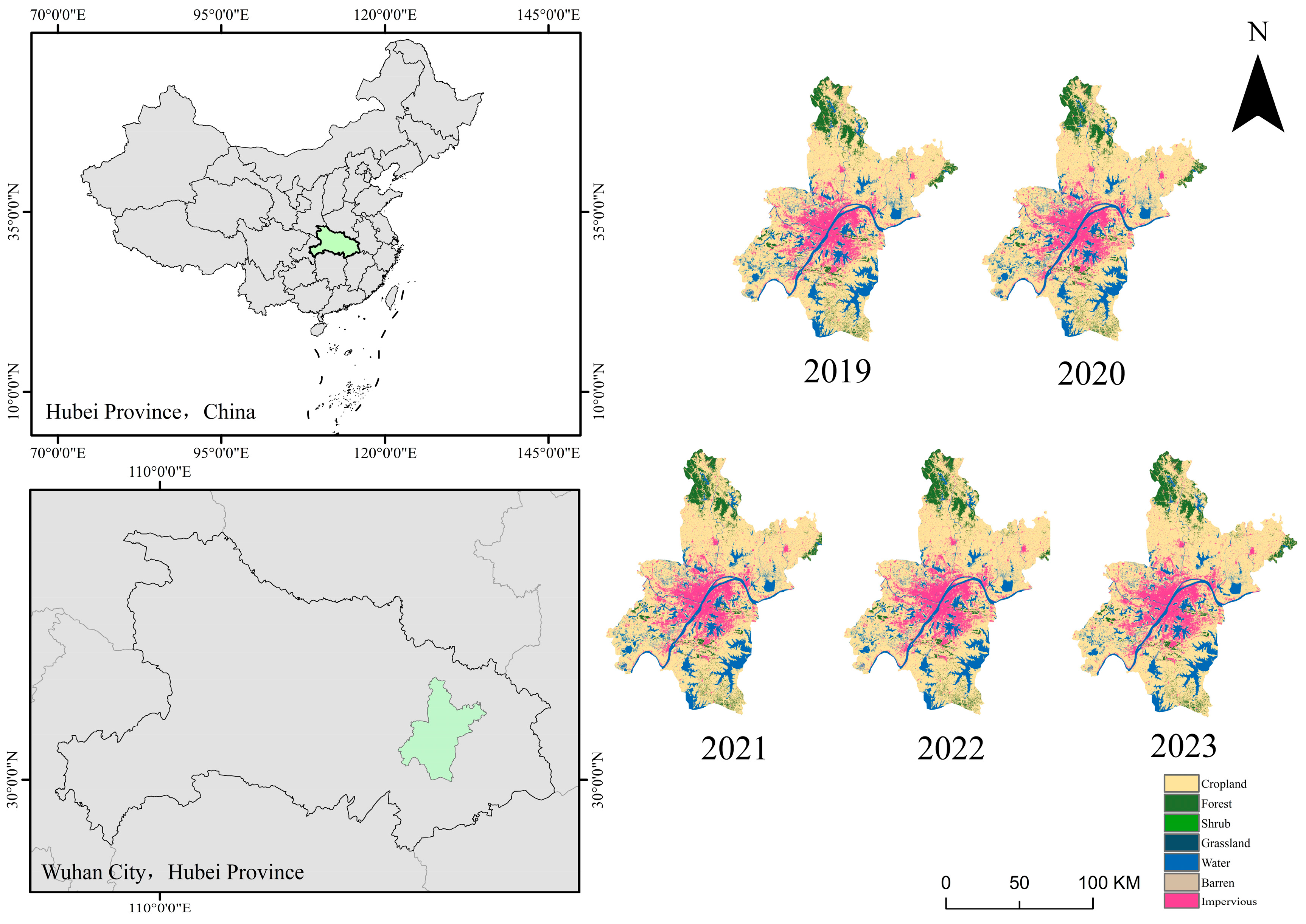
This research focused on Wuhan’s central urban area, a core metropolis in central China strategically positioned within the Yangtze River Economic Belt (see in Figure 1). Characterized by a subtropical humid monsoon climate with abundant precipitation, Wuhan features a unique hydrological landscape where the Yangtze River and its major tributary, the Han River, converge within the city core. Notably, over 200 lakes covering over 35% of the metropolitan area form an interconnected aquatic network. The study encompasses six central districts—Jiangan, Jianghan, Qiaokou, Hanyang, Wuchang, and Hongshan—spanning 589.83 km² and housing approximately 17.68 million residents as of 2023. Since 1980, rapid urbanization has transformed land cover through the conversion of cultivated land, grasslands, and bare earth to built-up land and water surfaces. Intensive economic growth and sustained population influx have driven vertical expansion, with high-rise structures and super-high-rise buildings now dominating the urban fabric. This spatial intensification has created distinctive micro-environments in high-density residential and commercial zones, establishing Wuhan as an exemplary case for studying compact urban form dynamics.

2.1.2. Selection of High-Density Communities

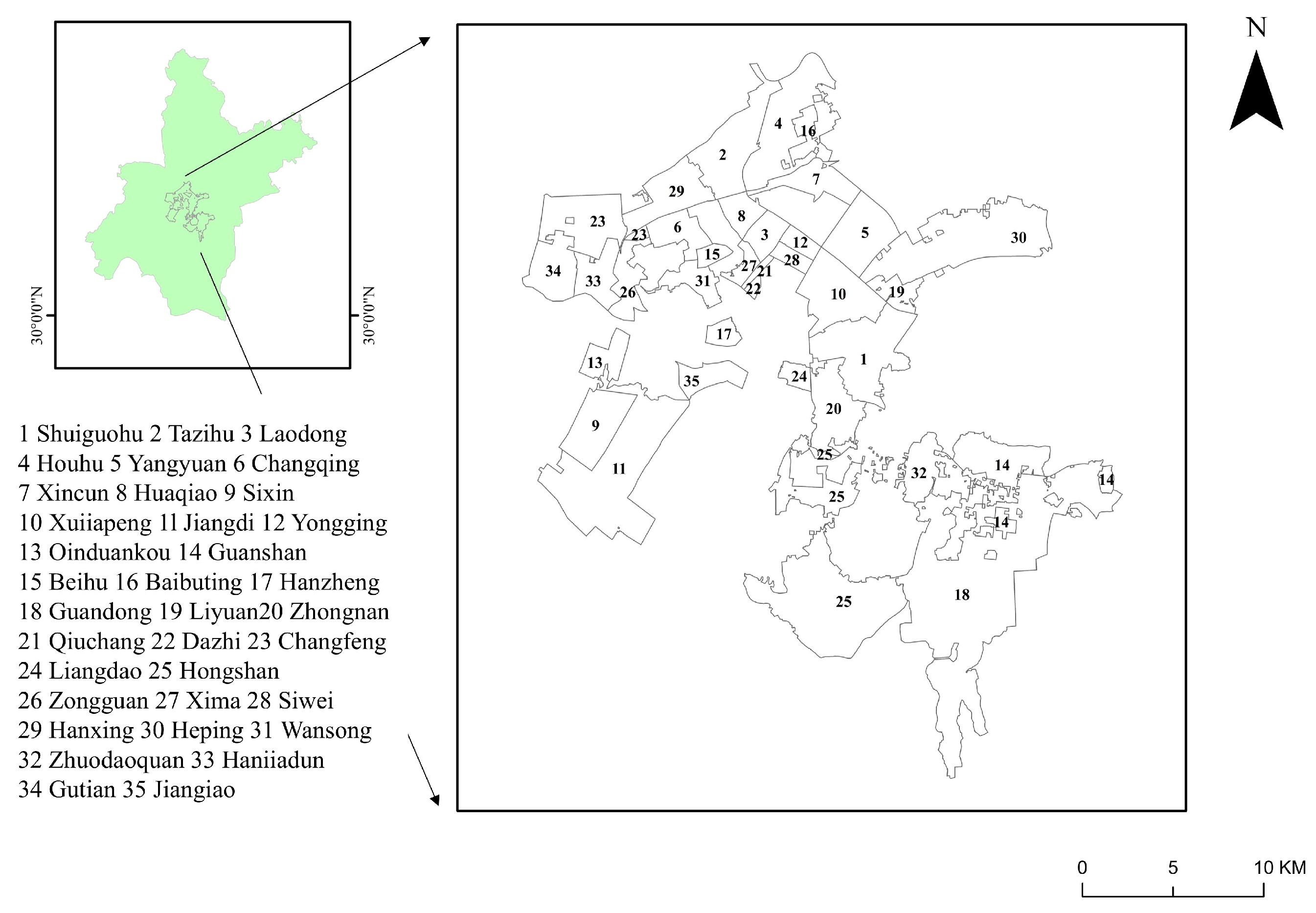
High-density communities are operationally defined as residential areas accommodating an elevated population density and built volumes within constrained land parcels. According to China’s 2018 Urban Residential Area Planning and Design Standards, such communities are defined as residential areas that exceed prescribed thresholds across key living-circle parameters, including maximum walking distances, population capacity limits, dwelling unit quotas, and floor area ratios. Complementing this, Wuhan’s 2020 Residential Land Construction Intensity Management Opinions established specific construction intensity controls for central urban areas (see

Table 1. Regulatory thresholds for residential intensity in Wuhan’s central urban area.

Control Indicators	Zoning of Residential Intensity
	Intensity Zone 1	Intensity Zone 2	Intensity Zone 3	Intensity Zone 4	Intensity Zone 5
Baseline floor area ratio	2.7	2.5	2.3	2.1	1.5
Maximum floor area ratio	3.0		2.5		2.0
Building density	D ≤ 20%		D ≤ 25%	D ≤ 30%	D ≤ 40%
Building height	H ≤ 100 m

). Combing above standards and academic definitions, we establish three diagnostic criteria for high-density residential areas: Baseline Floor Area Ratio > 2.5, Maximum Floor Area Ratio ≤ 3.0, and Building Density ≤ 20%. Furthermore, we define a high-density community as a spatial unit at street scale. Through geospatial validation using Gaode Map and Anjuke platforms, augmented by field verification, 35 streets that met all predefined criteria were identified (see in Figure 2). These selected streets serve as our research subjects.

2.2. Data Source

2.2.1. Landscape Pattern Indices

Landscape metric selection followed a multidimensional framework encompassing three core heterogeneity dimensions: compositional (type diversity), structural (patch geometry, edge effects), and configurational (spatial arrangement, connectivity) [46,47]. Based on the aforementioned three dimensions and previous research [48], this study selected patch density (PD), edge density (ED), Shannon’s diversity index (SHDI), and aggregation index (AI) as core indicators representing landscape patterns. Among these, SHDI reflects typological diversity within the compositional dimension; PD and ED together capture patch geometry and edge effects in the structural dimension; and AI exclusively characterizes spatial arrangement and connectivity in the configurational dimension. Each of these indicators carries unique and irreplaceable ecological significance within its respective dimension [49], collectively forming a comprehensive and non-redundant indicator system.

2.2.2. Land Use Data

The land use and land cover (LULC) data for Wuhan City spanning the period from 2019 to 2023 were obtained from the Global Surface Cover Database, which provides spatial resolution at 30 m (1.0.3, Vol. 13, Number 1, pp. 3907–3925) (https://zenodo.org/records/12779975, accessed on 1 May 2025). The dataset classifies land use types into nine distinct categories: cropland, forest, shrubland, grassland, water bodies, snow and ice, bare land, impervious surfaces, and wetlands [50].

2.2.3. Socioeconomic Factors

This study adopts four socioeconomic indicators at the street-level scale: population density (POP), gross domestic product (GDP_S), road density (RD), and nighttime light (NTL), with all calculations derived from street-level administrative units within Wuhan’s built-up area. Using ArcGIS 10.8, we performed spatial-temporal data fusion procedures to calculate these indicators for each street-level unit, as shown in

Table 2. Socioeconomic Indicators.

Socioeconomic Indicators	Calculation Formula	Data Source
POPD	$PO{P}_D={\displaystyle \frac{PO{P}_S}{A_S}}$	Land Scan dataset (https://landscan.ornl.gov, accessed on 12 May 2025)
GDPS	$GD{P}_S={\displaystyle \frac{PO{P}_S}{PO{P}_D}}GD{P}_D$	Wuhan Statistical Yearbook (https://tjj.wuhan.gov.cn/tjfw/tjnj/, accessed on 12 May 2025)
RD	$RD={\displaystyle \frac{L_S}{A_S}}$	Open Street Map (https://www.openstreetmap.org, accessed on 20 May 2025)
NTL	$NTL={\displaystyle \frac{{{\displaystyle \sum }}_{i=1}^{\mathrm{n}}D{N}_i}{n}}$	https://dataverse.harvard.edu/dataset.xhtml?persistentId=doi:10.7910/DVN/GIYGJU, accessed on 25 May 2025

Note: POP_S denotes the total population within a street segment boundary, person; A_S refers to the surface area of a street segment, km²; POP_D indicates the population density of containing county-level administrative unit, persons/km²; GDP_D represents the gross domestic product density of corresponding county-level administrative unit, ¥/km²; RD stands for road density, calculated as the ratio of total road length (L_S) to street segment area (A_S), km/km²; DN_i refers to the pixel radiance value for grid cell i; n represents total grid cells within study area.

.

2.3. Regression Model

Both the OLS regression and the GWR models were used to examine spatial relationships between landscape pattern metrics as dependent variables—specifically PD, ED, SHDI and AI—and socioeconomic indicators as independent variables, namely POP_D, GDP_S, RD, and NTL. Each landscape metric underwent separate univariate regression against individual socioeconomic predictors using both modeling approaches. Analyses were executed through ArcGIS 10.8’s regression tools, with all variables standardized via min–max normalization prior to modeling.

2.3.1. Spatial Autocorrelation

Spatial autocorrelation denotes the statistical dependence among observed variable values within a geographic distribution, where proximal locations may exhibit interdependent characteristics. The global Moran’s I index quantifies this spatial relationship, assessing the existence and magnitude of variable clustering across the study area. A statistically significant Moran’s I value confirms spatial dependence, indicating that geographically weighted regression modeling becomes methodologically appropriate for such data. The computation follows the formula as defined in reference [51].

$$I={\displaystyle \frac{{{\displaystyle \sum }}_{i=1}^s{{\displaystyle \sum }}_{j=1}^{\mathrm{s}}{w}_{ij}\left(x_i-\overline{x}\right)\left(x_j-\overline{x}\right)}{{{\displaystyle \sum }}_{i=1}^s{\left(x_i-\overline{x}\right)}^2}}$$

(1)

where I represents the global Moran’s I index within the range [−1, 1], where I > 0 indicates clustered patterns with increasing magnitude signifying stronger positive correlation, I < 0 denotes dispersed patterns with decreasing magnitude reflecting greater spatial disparity, and I = 0 confirms spatial randomness; s represents the total number of high-density community units comprising the study area; x_i and x_j are values of the explanatory variables at specific high-density community locations i and j; W_ij is the proximity-based spatial weight quantifying the connectivity strength between high-density communities i and j, typically derived from distance thresholds or contiguity relationships.

2.3.2. OLS Model

OLS is a conventional regression methodology characterized by globally fixed regression coefficients, implying that the relationships between variables remain consistent across all spatial locations. The calculation formulation of OLS is presented as follows [52]:

$$y={\beta }_0+{{\displaystyle \sum }}_{i=1}^{\mathrm{n}}{\beta }_i{x}_i+\epsilon$$

(2)

where y represents the dependent variable; β₀ denotes the global intercept constant; x_i corresponds to the value of the ith independent variable for the ith sample observation; β_i signifies the regression coefficient associated with the ith independent variable; n indicates the total number of independent variables; and ε represents the random error term accounting for unexplained variance.

2.3.3. GWR Model

GWR is an extension of the OLS regression method that incorporates spatially varying coefficients to account for spatial non-stationarity within the sample data. The model integrates geographical coordinates (u_i,v_i) of each observation point into its formulation [53], expressed as Equation (3) as follows:

$$y_i={\beta }_0\left({\mathrm{u}}_i,{\mathrm{v}}_i\right)+{{\displaystyle \sum }}_{j=1}^{\mathrm{n}}{\beta }_j\left({\mathrm{u}}_i,{\mathrm{v}}_j\right){\mathrm{x}}_{ij}+\epsilon$$

(3)

where y_i represents the dependent variable at spatial location i; u_i and vi denote the longitude and latitude coordinates of the ith location, respectively; β₀ (u_i,v_i) signifies the spatially varying intercept for the ith sample point; β_j (u_i,v_j) is the regression coefficient associated with the jth independent variable at the ith sample point; X_ij indicates the measured value of the jth independent variable at location i; and ε represents the random error component.

Additionally, GWR employs spatially variable weighting, where observations closer to the target location receive stronger influence on parameter estimation through distance-decay functions. This localized modeling approach constructs unique regression equations for each geographical unit by weighting neighboring observations according to their spatial proximity, effectively capturing spatial heterogeneity. Common weighting schemes include the Fixed Gaussian Kernel and the Adaptive Bi-square Kernel. The mathematical expression for the Fixed Gaussian function is written as follows:

$$W_{ij}=exp(-(d_{ij}^2/b^2))$$

(4)

where W_ij represents the spatial weight for observation j relative to target location i; d_ij is the Euclidean distance between locations i and j; and b denotes the kernel bandwidth determining the spatial scale of influence. In GWR modeling, two types of kernel functions are used: fixed and adaptive. In this study, since driving factors and their spheres of influence at the community level often operate at geographically consistent scales, the fixed kernel function was selected as a more suitable and robust option. The Akaike Information Criterion (AIC) serves as a selection criterion for determining the optimal bandwidth and evaluating model performance by balancing goodness of fit against model complexity. However, in cases of small sample sizes, AIC tends to exhibit significant bias toward overfitted models. In contrast, AICc effectively corrects this bias through an additional penalty term, making it a more reliable model selection criterion in GWR analysis [54].

3. Results

3.1. Evolutionary Characteristics of Landscape Patterns in Wuhan’s High-Density Communities

This study calculated landscape pattern metrics for the period of 2019–2023 using Fragstats 4.2 software, with the results presented in

Table 3. Comprehensive index of landscape pattern in high-density communities during 2019–2023.

Year	Landscape Pattern Metrics
	PD (number/hm2)	ED (m/hm2)	SHDI	AI (%)
2019	10.521	53.004	0.808	91.081
2020	10.524	52.478	0.802	91.159
2021	10.437	52.263	0.800	91.192
2022	10.303	50.456	0.790	91.463
2023	10.012	49.396	0.786	91.622

. According to Table 3, ED, PD, and SHDI exhibit consistent annual declines averaging 1.53%, 0.97% and 0.59%, respectively, while AI increased steadily at 0.11% per year. The positive correlation between decreasing PD and ED indicates progressive landscape consolidation with simplified patch boundaries, whereas the inverse relationship between rising AI and declining SHDI suggests aggregation processes reduce ecological diversity. A notable acceleration occurred in 2022, with PD decline intensifying from −1.3% to −2.8% and AI growth expanding from 0.15% to 0.27%, temporally coinciding with Wuhan’s 14th Five-Year Plan for Urban Renewal Initiatives. These metrics collectively demonstrate that anthropogenic landscape modification through urban expansion has exceeded natural succession processes in shaping landscape patterns during the study period.

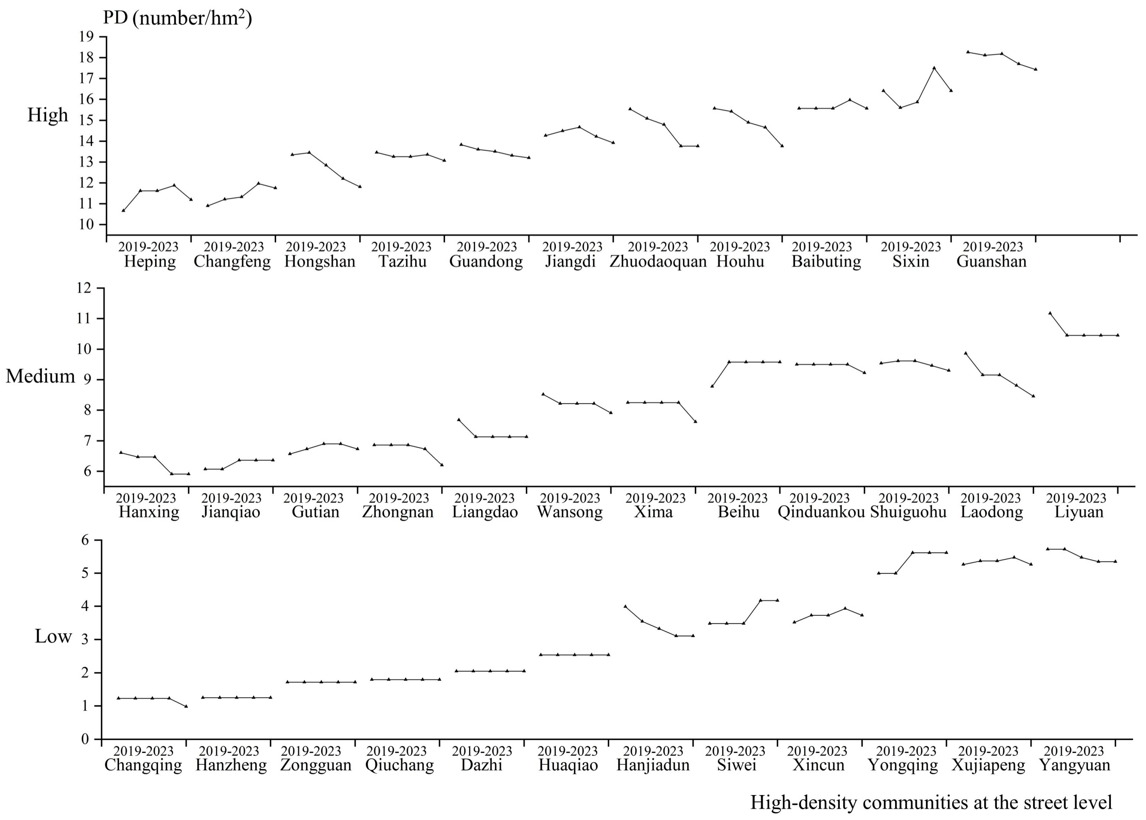
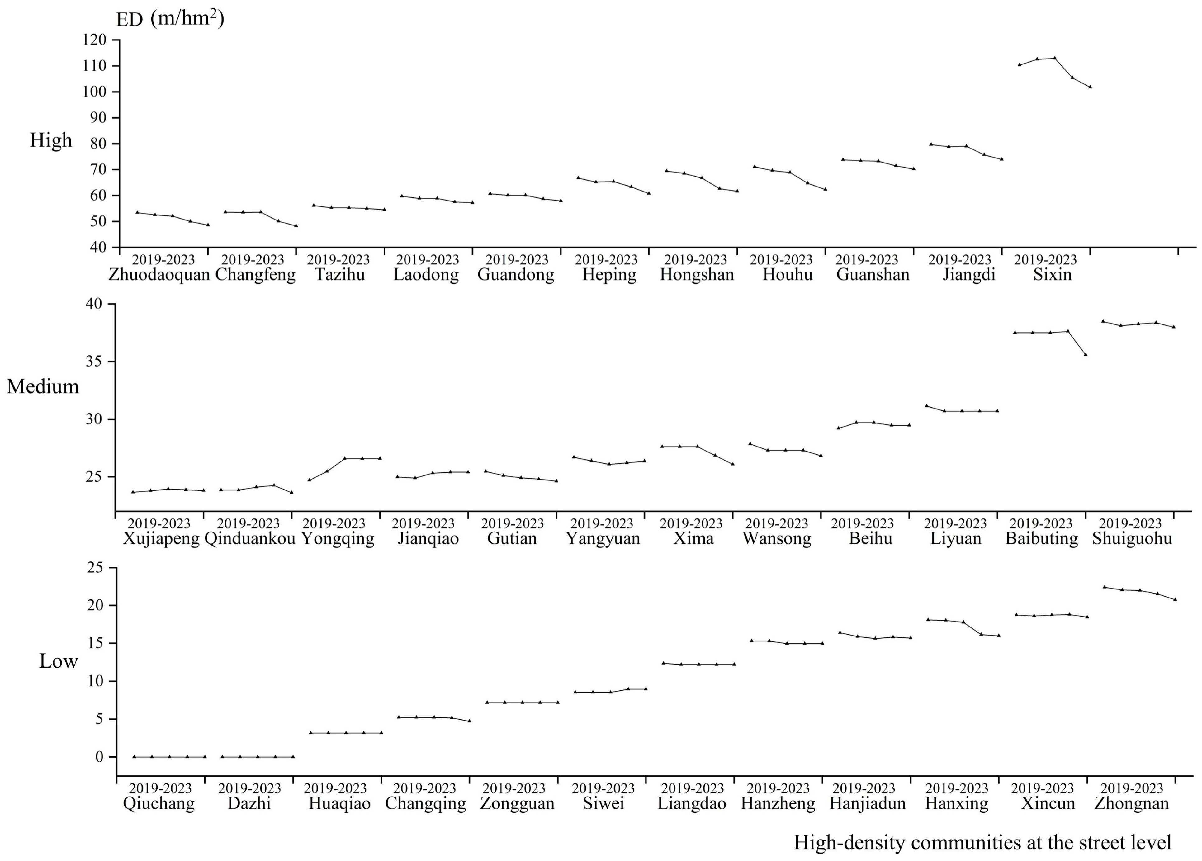
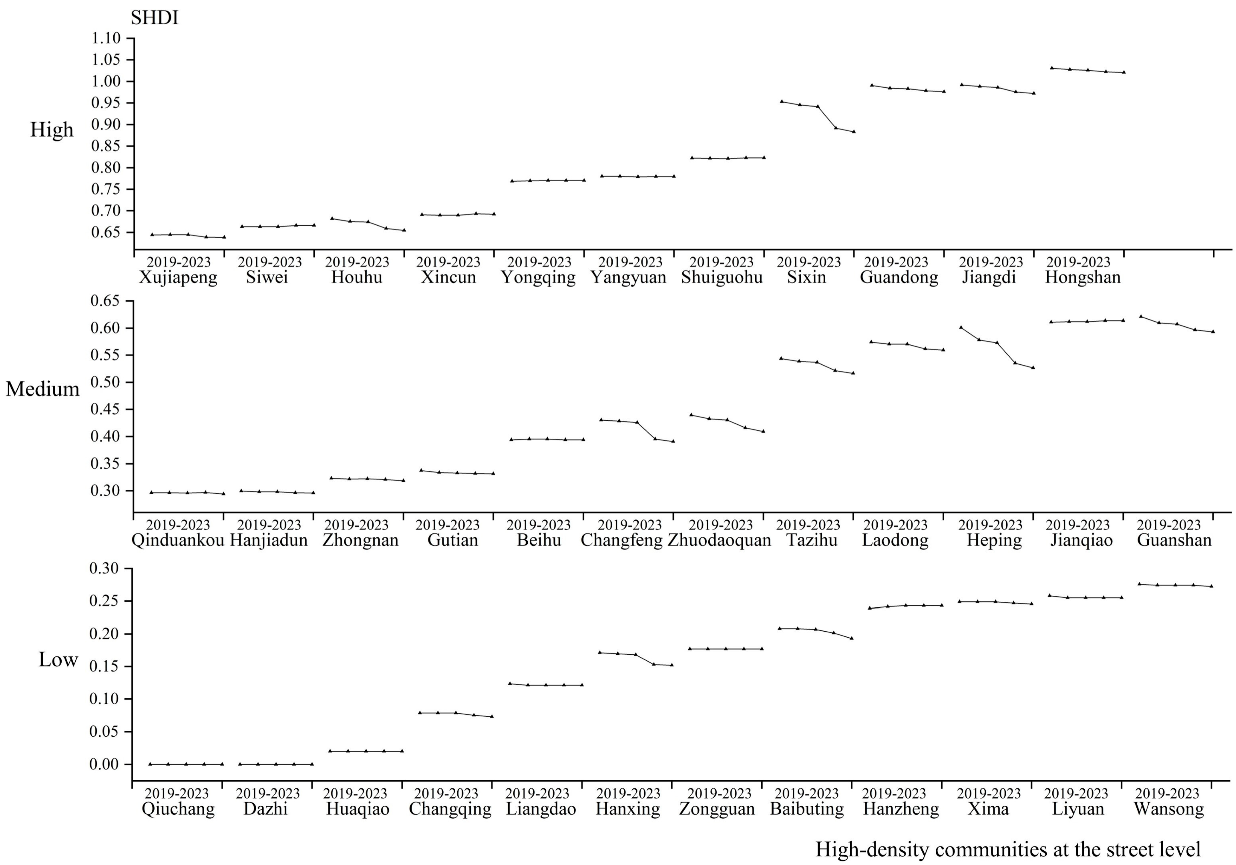
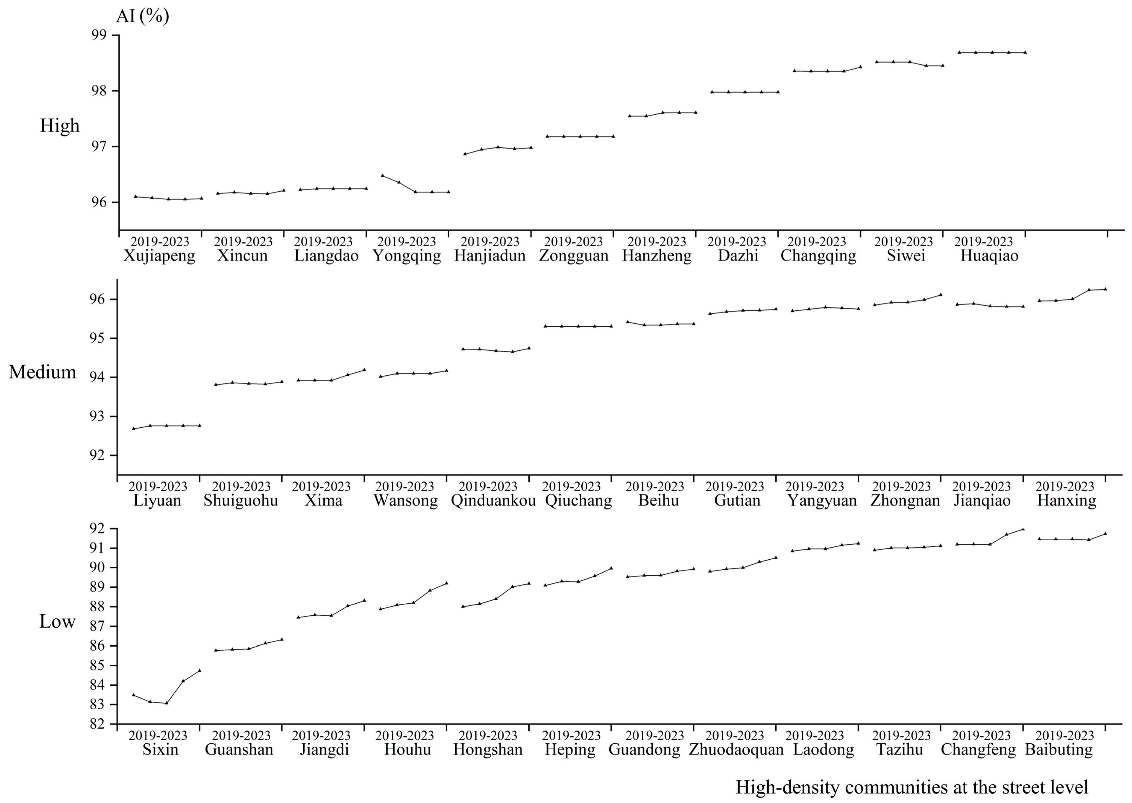
To investigate how urban renewal, infrastructure development and ecological restoration collectively influence landscape patterns, this study analyzed street-level spatiotemporal changes in four landscape indices—PD, ED, SHDI and AI—across high-density communities from 2019 to 2023. Moreover, to more effectively and clearly illustrate landscape dynamics and regional variations, the 35 streets were categorized into three groups (12, 12, and 11 units, respectively) and the landscape metrics were classified into three tiers—low, medium, and high—as shown in Figure 3, Figure 4, Figure 5 and Figure 6.

Figure 3 classified PD values into three distinct gradient intervals: low (0–6), medium (6–12), and high (12–19), revealing three key trends. First, most high-density communities exhibited declining PD values, particularly the Hongshan, Zhuodaoquan, Houhu, Laodong and Hanjiadun streets, where urban renewal and ecological restoration projects consolidated fragmented plots and enhanced patch connectivity. Second, nine communities, including the Heping and Changfeng streets, showed increasing PD values, primarily due to transportation infrastructure fragmenting green spaces and agricultural embankments disrupting aquatic ecosystems, exacerbating landscape fragmentation. Specifically, the Sixin street displayed an inverted N-shaped PD fluctuation: PD decreased from 2019 to 2020 due to the renovation of old neighborhoods and optimized land use efficiency, then increased between 2020 and 2022 owing to inefficient land development and road fragmentation, and declined again from 2022 to 2023 as a result of land redevelopment and ecological restoration. Third, six communities, including the Hanzheng and Zongguan streets, maintained stable PD values below three throughout the study period. Collectively, these observed patterns demonstrate human activities’ substantial influence on urban landscape evolution.

Figure 4 demonstrates distinct ED patterns across communities from 2019 to 2023. The majority of high-density communities displayed ED values within low (0–40) and medium (25–40) ranges, exhibiting varying characteristic trends: predominantly declining, partially stable, and minimally increasing patterns. For instance, the Hanxing and Baibuting streets showed significant ED declines, resulting from industrial-to-residential conversions that regularized plot geometry and improved spatial integration. In contrast, the Qiuchang and Dazhi streets consistently recorded zero ED values, indicating their uniform ecological structures with homogeneous landscapes. Notably, the Yongqing street displayed that initially, ED increased from urban renewal-induced fragmentation of natural patches into smaller construction parcels, followed by stabilization post-2021 when Wuhan’s construction land restrictions saturated the development capacity of this community and fixed its landscape configuration. Furthermore, among the 11 remaining communities with elevated ED values (40–120), most showed downward trends. Specially, the Sixin street, located in a core construction zone, sustained ED values above 100, initially rising (2019–2021) from intensive infrastructure expansion and inefficient land use before declining post-2021 through systematic plot consolidation and ecological restoration. These ED patterns demonstrate how land use changes, policy interventions, and ecological planning collectively reshape density community landscapes, highlighting both regulatory impacts on fragmentation and regional development variations.

Figure 5 reveals three distinct SHDI ranges across all communities: low (0–0.3), medium (0.3–0.65), and high (0.65–1), with 2019–2023 trends showing either stability or decline. Specifically, over 20 streets maintained stable SHDI values, as exemplified by the Qiuchang and Dazhi streets, where persistent zero values reflect uniform ecological structures. In contrast, the remaining streets exhibited declining SHDI values, signaling progressive landscape diversity loss due to urban functional specialization and concentrated land use patterns. Notably, the Heping, Sixin and Changfeng streets experienced the most pronounced decreases: Heping through road or block reconstruction, Sixin via wetland isolation from natural transition zones, and Changfeng by built-up area homogenization—all of which collectively replaced natural/semi-natural spaces with uniform industrial/commercial developments, thereby reducing ecological diversity. Ultimately, these trends demonstrate how systematic land use intensification and functional zoning fundamentally reconfigure ecological diversity patterns in urbanization.

Figure 6 reveals that from 2019 to 2023, most high-density communities had medium (92–96) to high (96–99) AI values, with only a minority falling in the low range (82–92). While most communities showed minor AI fluctuations due to small-scale interventions like greening upgrades that subtly modified land use patterns, others showed more pronounced trends. Notably, communities with AI values below 90 experienced significant increases as concentrated development enhanced the spatial aggregation of similar land uses. The Sixin street exemplified this upward trajectory after an initial decline, where transport infrastructure development (e.g., road expansion, Metro Line 12 construction) during 2019–2021 temporarily fragmented urban patches before subsequent infrastructure completion and ecological corridor establishment restored spatial aggregation. Conversely, streets like the Yongqing street showed marked AI decreases, resulting from urban renewal projects that introduced scattered, irregularly shaped features such as pocket parks and commercial outlets, thereby reducing spatial cohesion across the landscape.

In summary, the above reveals clear spatiotemporal heterogeneity in street-level landscape patterns across Wuhan’s high-density communities during 2019–2023, driven by integrated urban interventions, including renewal, plot consolidation, infrastructure expansion, ecological restoration, and zoning policies. The varied transformation pathways observed across dense communities emphasize the inherent complexity of ecological responses to urban land use change. To reconcile development with sustainability, future planning should prioritize multifunctional strategies that simultaneously optimize land use efficiency, ecological connectivity, and landscape diversity, ensuring synergistic alignment of urban structure and ecosystem functionality.

3.2. Spatiotemporal Heterogeneity in Landscape Patterns Driven by Socioeconomic Factors

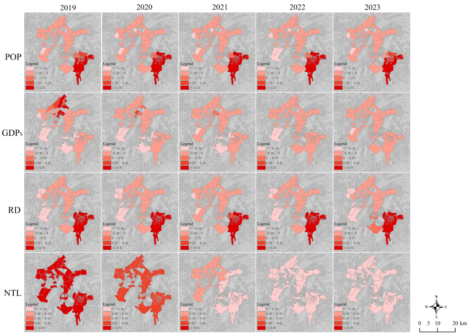
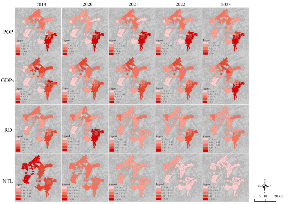
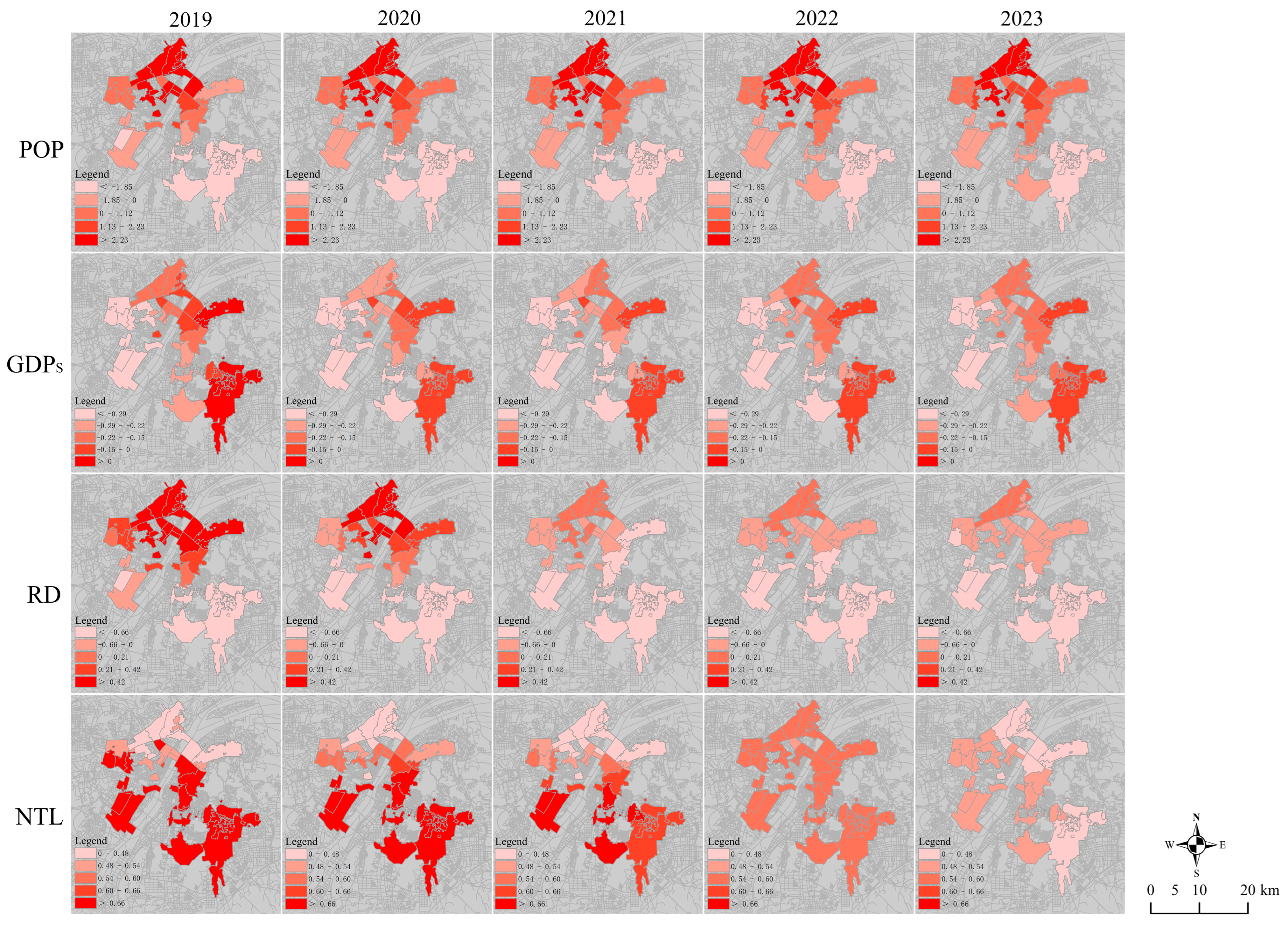
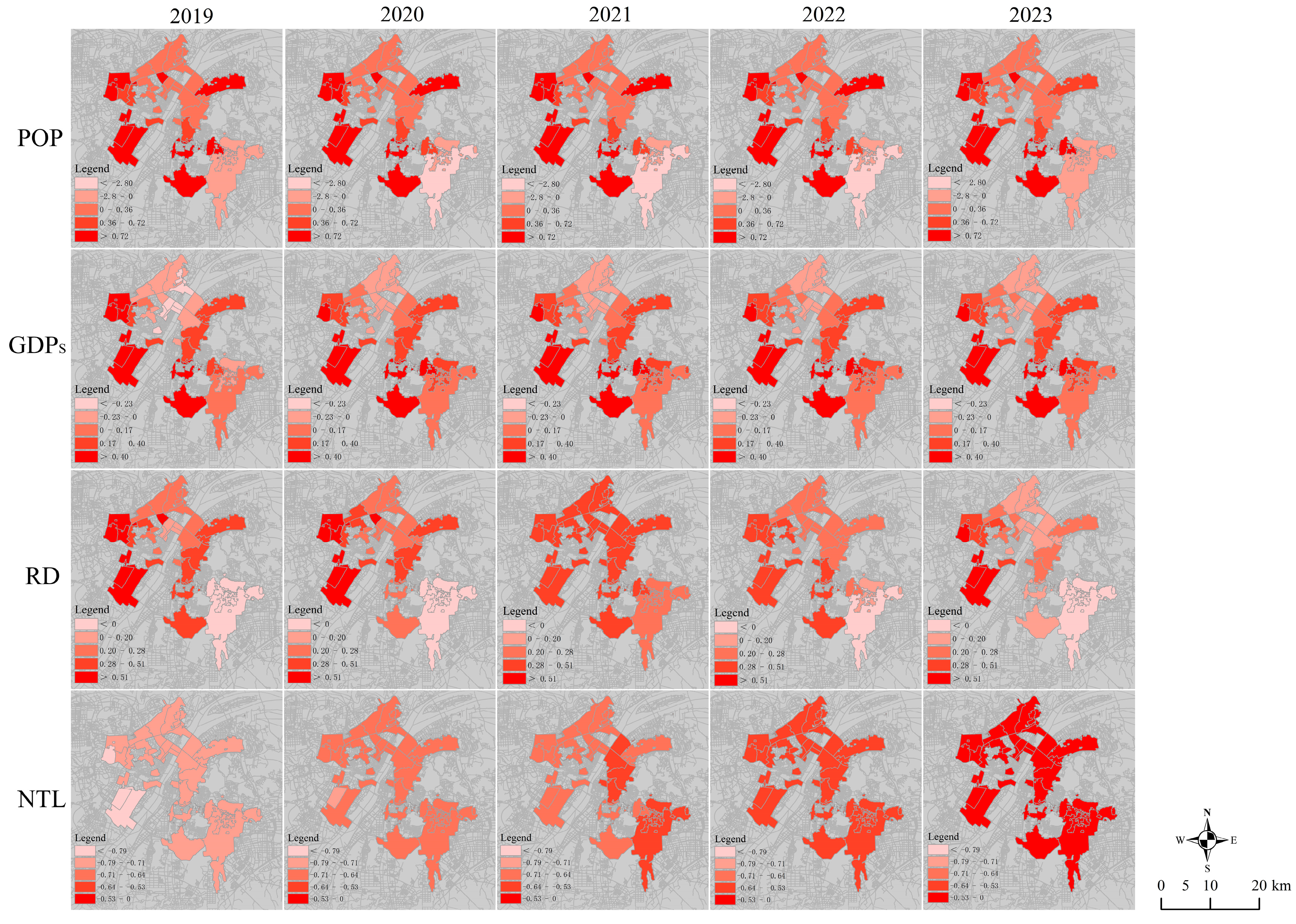
This study utilizes ArcGIS 10.8 and GWR modeling to quantify spatial non-stationarity in socioeconomic drivers (2019–2023), exploring their heterogeneous impacts on four landscape metrics: PD, ED, SHDI, and AI. Figure 7, Figure 8, Figure 9 and Figure 10 visualized the spatially varying regression coefficients (β), revealing localized effect magnitudes across the urban fabric.

For PD, Figure 7 reveals distinct socioeconomic influences: (1) POP generally exhibits a negative correlation with PD, averaging β = −0.48, suggesting that population concentration promotes landscape integration. Notably, the Gutian and Jiangdi streets demonstrate progressively intensifying negative POP-PD correlations (∆β = −0.21/year and −0.11/year, respectively), indicating their increasing effectiveness in suppressing landscape fragmentation through population concentration. However, exceptions such as the Guandong and Guanshan streets show a positive correlation (average β = +5.53 and +2.55, respectively), attributed to scattered expansion patterns. (2) GDPs primarily exerts negative effects on PD (average β = −0.20), with varying intensity across communities. Mature areas like the Yongqing and Qiuchang streets exhibit weak GDPs-induced fragmentation inhibition (β = −0.02 and −0.02, respectively), whereas economic zones like the Zhuodaoquan street show stronger negative effects (β = −0.52). Meanwhile, the Xincun (β = +0.07 in 2019 → −0.04 in 2023) and Laodong streets (β = +0.10 → −0.02) transitioned from positive to negative, signaling improved landscape integration driven by economic development. (3) RD generally reduces PD (average β = −0.33) by enhancing landscape connectivity in most communities. Yet, in the Guanshan and Guandong streets, RD correlates positively with PD (β = +0.56 and +0.56, respectively) due to the disordered road expansion that fragments the landscape. Moreover, stable temporal coefficients reflect the city’s shift from expansive growth to refined urban renewal. (4) NTL intensity consistently increases PD (average β = 0.56), linking elevated urban activity to landscape fragmentation. However, NTL’s regression coefficients decline annually with ∆β = −0.06/year, suggesting diminishing fragmentation impacts over time due to stabilized urban structures or green planning interventions.

For ED, Figure 8 reveals that: (1) POP predominantly exhibits a negative association with ED (average β = −0.77), demonstrating the land plot regularization and edge simplification effects of concentrated development. However, certain communities display positive POP-ED relationships, wherein population growth drives the expansion of fragmented construction land and increased edge complexity. A notable example is the Guanshan street, where the POP–ED relationship transitioned from negative (2019: β = −0.00028) to positive (2021: β = +1.05) and subsequently to a weakened effect (2023: β = +0.17), reflecting progressive urban renewal implementation. (2) GDPs displays divergent effects on ED across communities: reducing ED in the Sixin (β = −1.22) and Jiangdi streets (β = −0.82) through land integration and edge simplification, while increasing ED in the Guandong (β = +0.20) and Yongqing streets (β = +0.12) via irregular development patterns. Notably, the Guanshan street undergoes a progressive transition from a positive GDPs–ED correlation in 2019 (β = +0.29) to a negative correlation by 2023 (β = −0.05), signaling enhanced landscape integration associated with the maturing economic activities. (3) RD typically exhibits a negative correlation with ED (average β = −0.43), reflecting that road network development contributes to spatial structure optimization and landscape boundary simplification. Notably, the Guandong street displayed a three-phase evolution: during initial construction (2019), RD reduced ED (β = −0.10) through systematic plot integration; subsequent scattered expansion (2020) increased edge complexity (β = +0.26) due to uncoordinated development; and post-2021 urban renewal restored negative correlation (β = −0.48) through integrated infrastructure planning, showcasing how phased interventions can progressively enhance landscape connectivity. (4) NTL intensity shows a consistently positive correlation with ED across all communities (average β = +0.64), linking heightened urban activity to greater landscape edge complexity. However, the effect diminished over time (∆β = −0.07/year), reflecting the progressive stabilization of urban form as development matures, and successful mitigation through green infrastructure investments and compact city planning. This attenuation is particularly evident in communities like the Sixin street, where NTL-ED coefficients declined from β = +0.79 (2019) to β = +0.51 (2023), validating the effectiveness of light pollution reduction strategies and spatial planning interventions.

For SHDI, Figure 9 demonstrates that: (1) POP exhibits a significant negative correlation with SHDI (β = −1.33, p < 0.01), reflecting that urban densification reduces landscape heterogeneity through land use intensification and functional homogenization. The Hongshan street exemplifies a promising mitigation trend, where the POP–SHDI effect has attenuated annually (∆β = +0.07/year), declining form β = −3.95 in 2019 to β = −3.67 in 2023. This decoupling reflects the successful implementation of targeted ecological preservation policies, alongside improved land use efficiency achieved through mixed-use zoning. (2) GDPs demonstrates transitional effects on SHDI: the Guanshan (β = +0.21 → −0.15) and Guandong streets (β = +0.55 → −0.13) show clear economic encroachment through their positive-to-negative coefficient shifts, while the Beihu (β = −0.261 ± 0.015) and Changqing streets (β = −0.307 ± 0.017) maintained stable ecological integration despite development pressures. (3) RD predominantly shows a persistent negative correlation with SHDI (mean β = −0.50, p < 0.01), demonstrating that road network expansion drives landscape homogenization through geometric regularization of land parcels, fragmentation of ecological patches, and centralized development patterns. This trend is particularly pronounced in the Hanzheng street, where RD–SHDI coefficients intensify from β = −0.34 (2019) to β = −0.48 (2023) (∆β = −0.03/year), indicating accelerating diversity loss from sustained road infrastructure development. (4) NTL positively correlates with SHDI (β = +0.55, p < 0.01), indicating that urban activity enhances diversity through mixed land functions and structural heterogeneity. Concurrently, the annually weakening relationship (∆β = −0.08/year) reveals an important transition where stabilizing urban structures and implemented green policies gradually reduce these diversity fluctuations as the development matures, as exemplified by the Sixin street’s decline from β = +0.98 (2019) to β = +0.49 (2023).

For AI, Figure 10 demonstrates that: (1) POP exhibits a predominant positive correlation with AI across high-density communities (β = +0.47, p < 0.05), reflecting urban renewal and land use restructuring driven by population growth, enhancing patch consolidation. However, the Guanshan street exemplifies a characteristic mitigation pattern, where the POP–AI relationship transitioned from strong negative effects (β = −0.74 in 2019) to progressively weaker impacts (β = −1.08 in 2023, ∆β = +0.09/year), reflecting how progressive environment upgrades and ecological interventions can mitigate population-driven disaggregation. (2) GDPs demonstrates divergent AI relationships. Most communities, including mature communities like the Shuiguohu (β = + 0.23) and Changqing streets (β = +0.13), show persistent positive correlations through concentrated functional zoning and stable land use. Conversely, a minority exhibited a weakening negative effect (e.g., the Baibuting street: β = −0.23 → −0.03; the Yongqing street: β = −0.37 → −0.08) as infill development mitigates residential fragmentation. Specifically, the Yangyuan street’s transition from negative (β = −0.06, 2019) to positive GDPs–AI correlations (β = +0.05, 2023) highlights how rapid economic growth can eventually enhance spatial aggregation when accompanied by strategic planning interventions. (3) RD generally increases AI (β = +0.28) through improved connectivity. For instance, the Houhu street shows a characteristic rise-and-decline pattern in road network efficacy—initial infrastructure expansion (2019–2021) significantly improved connectivity (peak β = +0.32 in 2020), followed by diminishing aggregation returns by 2023 (β = +0.22) as the network approached saturation. (4) NLT negatively correlates with AI across most communities (β = −0.63, p < 0.01), as frequent nocturnal activity fragments land plots and mixes functions, reducing patch cohesion. For instance, the Sixin (β = −0.79 to −0.51) and Jiangdi streets (β = −0.79 to −0.50) both show weakening negative trends (∆β = +0.07/year), confirming the effectiveness of implemented light pollution controls and green space renovations in stabilizing landscape patterns.

In summary, the above reveals pronounced spatiotemporal heterogeneity in how socioeconomic factors shape urban landscape patterns. POP and RD directly reduce fragmentation through physical development integration, while GDPs and NLT indirectly influence patterns via economic restructuring and land use changes. NTL particularly enhances fragmentation and edge complexity. These drivers collectively generate distinct spatial patterns across high-density communities, as demonstrated by our geographically varying regression analyses.

4. Discussion

4.1. Spatial Autocorrelation Analysis of Variables

Moran’s I measures spatial autocorrelation and assesses whether regression model assumptions follow a random spatial distribution. It is widely used to validate regression model fit [55].

Table 4. Moran’s I index, z-value, and p-value of variables.

Year	Degree	Variables
		PD	ED	SHDI	AI	POP	GDPS	RD	NTL
2019	Moran’s I	0.408	0.297	0.349	0.303	0.649	0.718	0.509	0.205
	z-value	3.08	2.42	2.69	2.43	5.69	5.4	4.40	1.67
	p-value	***	***	***	***	***	***	***	**
2020	Moran’s I	0.398	0.300	0.348	0.306	0.659	0.241	0.498	0.107
	z-value	3.01	2.46	2.67	2.47	5.63	1.98	4.26	0.98
	p-value	***	***	***	**	***	**	***
2021	Moran’s I	0.397	0.302	0.347	0.308	0.659	0.242	0.426	0.141
	z-value	0.01	2.48	2.67	2.48	5.63	1.98	3.58	1.23
	p-value	***	**	***	**	***	**	***
2022	Moran’s I	0.373	0.308	0.348	0.313	0.659	0.254	0.421	0.194
	z-value	2.86	2.51	2.67	2.51	5.63	2.07	3.57	1.65
	p-value	***	**	***	**	***	**	***	*
2023	Moran’s I	0.381	0.309	0.345	0.315	0.674	0.347	0.472	0.271
	z-value	2.91	2.51	2.65	2.52	5.61	2.75	3.95	2.24
	p-value	***	**	***	**	***	***	***	**

***, **, and * represent 1%, 5%, and 10% significance levels, respectively; blank space represent no significance.

shows Moran’s I values ranging from 0.107 to 0.718. For all dependent variables (PD, ED, SHDI, AI) and independent variables (POP, GDPS, RD), p-values are below 0.05, and z-values exceed 1.96, confirming significant spatial autocorrelation at the 5% level. This indicates clear spatial clustering patterns. The independent variable NTL exhibit p-values between 0.027 and 0.117, suggesting weak clustering in some areas. However, due to the limited sample size (n = 35), statistical power is insufficient to reject spatial randomness. These results justify using the GWR model to analyze relationships between the dependent variables (PD, ED, SHDI, AI) and independent variables (POP, GDPS, RD, NTL).

4.2. Performance Comparison Between OLS and GWR Models

We evaluated model performance using adjusted R² and AICc. A higher adjusted R² indicates stronger explanatory power of the independent variables, while a smaller AICc suggests a better fit of the model to the observed data. Furthermore, to compare the ability of OLS and GWR models to handle spatial autocorrelation of variables, the global Moran’s I of the residuals of both models was calculated. The global Moran’s I reflects spatial similarity between adjacent or neighboring units and can detect spatial autocorrelation in model residuals. The value of Moran’s I ranges from −1 to 1; a value close to −1 indicates negative spatial autocorrelation, a value close to 1 indicates positive spatial autocorrelation, and a value close to 0 suggests little or no spatial autocorrelation. If the residuals from the regression model show significant spatial autocorrelation, it violates the assumption of residuals being randomly distributed. The spatial autocorrelation tool in ArcGIS 10.8 was used to count and compare the Moran’s I of the residuals from both models.

Both the OLS and the GWR models can generate adjusted R² values, AICc and residual Moran index for each study area. As shown in

Table 5. Comparison between the adjusted R2 values of the GWR (R²G) and OLS (R²O) models.

		2019				2020				2021				2022				2023
		POP	GDPS	RD	NTL	POP	GDPS	RD	NTL	POP	GDPS	RD	NTL	POP	GDPS	RD	NTL	POP	GDPS	RD	NTL
PD	R2O	0.182	0.012	0.170	0.298	0.190	0.059	0.175	0.269	0.272	0.061	0.097	0.272	0.192	0.078	0.079	0.224	0.209	0.095	0.074	0.262
	R2G	0.577	0.448	0.490	0.320	0.603	0.428	0.520	0.292	0.605	0.410	0.424	0.295	0.600	0.399	0.394	0.249	0.609	0.419	0.410	0.285
ED	R2O	0.204	0.020	0.217	0.388	0.210	0.066	0.229	0.345	0.362	0.063	0.166	0.362	0.217	0.070	0.164	0.331	0.240	0.080	0.150	0.348
	R2G	0.695	0.638	0.363	0.408	0.715	0.483	0.520	0.366	0.715	0.491	0.193	0.383	0.713	0.485	0.200	0.353	0.699	0.522	0.189	0.386
SHDI	R2O	0.266	0.019	0.221	0.349	0.278	0.053	0.244	0.314	0.311	0.057	0.261	0.311	0.270	0.057	0.265	0.325	0.2940	0.066	0.257	0.304
	R2G	0.793	0.316	0.387	0.559	0.745	0.254	0.424	0.424	0.744	0.244	0.392	0.428	0.739	0.234	0.400	0.347	0.753	0.234	0.366	0.326
AI	R2O	0.088	0.011	0.111	0.381	0.094	0.069	0.116	0.332	0.346	0.063	0.064	0.346	0.093	0.071	0.054	0.323	0.110	0.090	0.046	0.357
	R2G	0.628	0.663	0.495	0.400	0.689	0.499	0.506	0.354	0.665	0.500	0.193	0.367	0.661	0.494	0.233	0.344	0.630	0.531	0.400	0.379

,

Table 6. Comparison between the AICc values of the GWR (AICcG) and OLS (AICcO) models.

		2019				2020				2021				2022				2023
		POP	GDPS	RD	NTL	POP	GDPS	RD	NTL	POP	GDPS	RD	NTL	POP	GDPS	RD	NTL	POP	GDPS	RD	NTL
PD	AICcO	99.2	105.8	99.7	93.8	98.0	103.3	98.7	94.5	97.5	102.7	101.4	93.8	97.4	102.0	102.0	96.0	94.4	99.2	100.0	92.0
	AICcG	100.8	103.4	101.9	94.9	102.4	102.7	98.8	95.6	101.7	101.8	103.2	94.9	102.1	102.4	104.7	97.1	99.2	99.2	101.6	93.1
ED	AICcO	99.0	106.3	98.4	89.8	98.5	104.4	98.7	92.0	98.4	104.3	100.3	90.9	94.1	100.2	96.4	88.6	91.0	97.7	95.0	85.7
	AICcG	94.8	106.6	99.0	90.8	96.4	101.9	98.6	93.1	96.1	101.8	101.3	92.0	92.5	98.2	97.4	89.6	88.0	96.7	95.8	86.5
SHDI	AICcO	94.7	104.2	96.8	90.5	93.7	103.3	95.4	92.0	93.7	103.0	94.5	92.0	93.3	102.3	93.6	90.5	92.0	101.8	93.8	91.5
	AICcG	92.9	103.1	96.7	101.8	90.9	102.6	94.8	95.4	90.8	102.6	94.9	95.7	90.7	101.9	93.7	91.6	89.0	101.7	94.0	92.6
AI	AICcO	103.8	106.6	102.8	90.2	103.3	104.2	102.4	92.6	103.1	104.3	104.2	91.7	99.3	100.2	100.8	89.1	96.6	97.4	99.0	85.2
	AICcG	96.7	102.3	104.1	91.3	99.4	98.8	101.0	93.7	97.6	98.5	104.1	92.7	94.2	94.8	99.8	90.2	90.3	92.7	97.8	86.2

and

Table 7. Comparison between the residual Moran’s I index of the GWR (IG) and OLS (IO) models.

		2019				2020				2021				2022				2023
		POP	GDPS	RD	NTL	POP	GDPS	RD	NTL	POP	GDPS	RD	NTL	POP	GDPS	RD	NTL	POP	GDPS	RD	NTL
PD	IO	0.123	0.270	0.124	0.072	0.117	0.248	0.124	0.094	0.113	0.235	0.175	0.087	0.106	0.222	0.167	0.101	0.095	0.233	0.162	0.093
	IG	0.040	0.179	0.057	0.071	0.04-	0.163	0.049	0.093	0.029	0.161	0.102	0.086	0.032	0.156	0.093	0.101	0.021	0.151	0.077	0.093
ED	IO	0.079	0.200	0.076	0.037	0.074	0.171	0.071	0.057	0.073	0.163	0.118	0.054	0.073	0.162	0.110	0.061	0.064	0.164	0.102	0.063
	IG	−0.031	0.088	0.059	0.037	−0.040	0.084	0.014	0.056	−0.041	0.086	0.117	0.054	−0.042	0.084	0.108	0.061	−0.040	0.068	0.010	0.064
SHDI	IO	0.107	0.134	0.135	0.141	0.010	0.099	0.126	0.154	0.010	0.089	0.167	0.158	0.102	0.085	0.148	0.153	0.101	0.081	0.134	0.155
	IG	−0.029	0.080	0.105	0.079	−0.015	0.069	0.097	0.128	−0.015	0.065	0.141	0.129	−0.013	0.062	0.125	0.153	−0.013	0.056	0.118	0.155
AI	IO	0.120	0.205	0.105	0.039	0.113	0.168	0.103	0.060	0.112	0.163	0.112	0.058	0.114	0.161	0.147	0.060	0.105	0.160	0.143	0.058
	IG	0.046	0.108	0.043	0.038	0.019	0.093	0.035	0.060	0.028	0.098	0.127	0.058	0.030	0.096	0.120	0.060	0.035	0.076	0.070	0.058

, GWR demonstrates a superior performance with adjusted R² values ranging from 0.189 to 0.919, which is significantly higher than OLS’s range of 0.012 to 0.388. GWR’s AICc values ranging from 85.2 to 106.6 remain comparable to OLS’s, due to its requirement for estimating location-specific independent parameters like intercepts and slopes. This similarity arises because GWR’s parameter count approaches the sample size (n = 35), inflating model degrees of freedom. The Moran’s I index of the OLS model ranged from −0.04 to 0.27, while that of the GWR model ranged from −0.04 to 0.179 and was consistently lower than that of the corresponding OLS model. More importantly, the residual Moran’s I of the GWR model was significantly closer to zero in all instances, indicating that the GWR model effectively captures spatially varying relationships and accounts for the spatial autocorrelation of variables. Furthermore, we conducted the Koenker test on the residuals of the OLS model and detected the presence of heteroscedasticity in some variables, which further validates the necessity of employing a GWR model. The analysis confirms GWR’s stronger performance in modeling spatial relationships between landscape patterns and their driving factors, while OLS maintains its utility for evaluating broader, study-area-wide patterns.

4.3. Policy Implication for High-Density Communities

Amidst rapid global urbanization, high-density communities have developed along diverse pathways. Research indicates that the development drivers in Wuhan exhibit significant spatial heterogeneity. While population and economic factors serve as core driving forces, their influence varies considerably across different communities, highlighting the need for more refined and differentiated urban planning policies that adapt to local conditions. Compared to the market-led development model predominant in North America and the strict regulatory approach emphasizing historical preservation in European cities, Wuhan places greater emphasis on government-led initiatives, functional zoning, and the coordinated development of a polycentric structure. In contrast to other high-density Asian cities, Wuhan focuses more on scale effects and multi-center balance.

This study employs the GWR model to investigate the driving relationships between socioeconomic factors and landscape patterns, offering critical policy insights for green high-density communities planning.

• Strengthening ecological corridor construction and optimizing the structure of community green spaces. Between 2019 and 2023, Wuhan’s high-density communities experienced significant declines in ED and SHDI, reflecting reduced landscape connectivity and biodiversity during urban land conversion. In order to offset these impacts, Wuhan has accelerated the construction of the Baili Yangtze River Ecological Corridor, continued to promote the gate reconstruction of the urban section and the riverside green road connection project, connected the scattered beach parks, and formed a continuous and complete waterfront ecological space. At the same time, Wuhan has vigorously promoted the greening and reconstruction of old residential areas, and expanded the green ecological space by planning and building green buildings, removing walls to show green, removing and returning green buildings, and planting green plants on mountains. These enhancements simultaneously improve recreational access and strengthen urban ecological functionality.
• Developing community-level specific strategies according to their distinct socioeconomic drivers. The spatial heterogeneity of socioeconomic influence on landscape patterns requires differentiated planning strategies in high-density communities. Where population growth intensifies fragmentation, mixed land use approaches should optimize efficiency. Where it promotes green space integration, multi-layered vegetation systems—with tree canopies, shrub understories, and herbaceous groundcover—should enhance biodiversity. Thus, decision-makers should adopt adaptive governance frameworks to simultaneously achieve land use efficiency and ecological resilience.
• Exploring innovative ecological compensation paths, such as vertical greening and micro-ecological space construction. The evolution of landscape patterns in Wuhan’s high-density communities exhibited increasingly simplified land use types alongside strengthened socioeconomic correlations from 2019 to 2023, reflecting both post-pandemic sustainable transitions and heightened governmental emphasis on ecological functionality. Thus, policymakers should formalize innovative practices through robust governance frameworks, enhanced planning incentives, and standardized ecological compensation mechanisms to accelerate urban ecosystem sustainability.

5. Conclusions

Amid rapid global urbanization, high-density communities—serving as crucial hubs for population agglomeration, economic activity, and cultural exchange—are undergoing profound transformations. This study employed landscape pattern indices and the GWR model to analyze the evolution of street-level urban landscapes and their socioeconomic drivers in Wuhan’s high-density communities, with a particular focus on spatial heterogeneity. Results demonstrate that the evolution trends of landscape patterns reflected how policy interventions, engineering practices, and spatial governance collectively shape landscape patterns. The spatial morphological changes can be operationalized through urban greening projects and ecological infrastructure development, providing a foundation for systematically enhancing ecological diversity via land use intensification and functional zoning. Among the driving factors, POP and RD demonstrated a direct influence on landscape patterns, whereas GDP_S and NTL influenced patterns indirectly through economic restructuring, land use changes, and policy-driven investments. Wuhan’s practical experience highlights the importance of exploring innovative compensation mechanisms for vertical greening and micro-ecological spaces, while enforcing green space protection and expanding urban green landscapes. This study provides a transferable framework for the planning and governance of other high-density cities, urging planners to extend strategies from the macro-urban level to the community level for targeted interventions. Furthermore, by adopting a community-scale perspective, it captures micro-scale changes that are often overlooked in high-density urban research, offering valuable insights for balancing development and sustainability in other cities. It also contributes meaningful theoretical and practical guidance for enhancing ecological resilience and sustainability in high-density urban areas.

Spatial scale is one of the central issues in ecology and geography. Since landscape patterns are scale-dependent, changes in these patterns and their driving forces are also sensitive to the granularity or extent of observation. The current limitations imposed by a spatial resolution of 30 m in land cover data and the administrative granularity at street level units constrain micro-scale analytical capabilities. Future research endeavors should prioritize: (1) land cover data with 10 m resolution; (2) expanding the temporal scope to effectively capture long-term landscape dynamics; and (3) integrating GWR models with machine learning algorithms to enhance the capability of models in handling complex data.

References

1. Li, J.; Wei, X.; Shen, L. Analysis on the Synchronized Development between Urbanization Process and Eco-Efficiency through the Sustainability Lens. Environ. Sci. Pollut. Res. 2023, 30, 80828–80843. [Google Scholar] [CrossRef]
2. Shi, Y.; Zheng, Y.; Chen, D.; Yang, J.; Cao, Y.; Cui, A. Research on the Correlation between the Dynamic Distribution Patterns of Urban Population Density and Land Use Morphology Based on Human–Land Big Data: A Case Study of the Shanghai Central Urban Area. Land 2024, 13, 1547. [Google Scholar] [CrossRef]
3. Chen, Y.; Men, H.; Ke, X. Optimizing Urban Green Space Patterns to Improve Spatial Equity Using Location-Allocation Model: A Case Study in Wuhan. Urban For. Urban Green. 2023, 84, 127922. [Google Scholar] [CrossRef]
4. Huang, Y.; Lieske, S.N.; Wang, S.; Liu, Y. How Does Heterogeneity in Dwelling Type Preferences Relate to Housing and Built Environment Characteristics? Int. J. Digit. Earth 2023, 16, 93–112. [Google Scholar] [CrossRef]
5. McDonnell, M.J.; Pickett, S.T.A. Ecosystem Structure and Function Along Urban-Rural Gradients: An Unexploited Opportunity for Ecology. Ecology 1990, 71, 1232–1237. [Google Scholar] [CrossRef]
6. Lepczyk, C.A.; Aronson, M.F.J.; Evans, K.L.; Goddard, M.A.; Lerman, S.B.; MacIvor, J.S. Biodiversity in the City: Fundamental Questions for Understanding the Ecology of Urban Green Spaces for Biodiversity Conservation. Bioscience 2017, 67, 799–807. [Google Scholar] [CrossRef]
7. Magura, T.; Ferrante, M.; Lövei, G.L. Only Habitat Specialists Become Smaller with Advancing Urbanization. Glob. Ecol. Biogeogr. 2020, 29, 1978–1987. [Google Scholar] [CrossRef]
8. Meng, Z.; Mo, X.; Xue, Q.; Wang, Z.; Lu, X.; Liu, J.; Ma, Q.; Sparks, J.P.; He, M. Distribution, Source Apportionment, and Ecological Risk Assessment of Soil Antibiotic Resistance Genes in Urban Green Spaces. Environ. Res. 2024, 251, 118601. [Google Scholar] [CrossRef] [PubMed]
9. Xing, L.; Chen, Q.; Liu, Y.; He, H. Evaluating the Accessibility and Equity of Urban Health Resources Based on Multi-Source Big Data in High-Density City. Sustain. Cities Soc. 2024, 100, 105049. [Google Scholar] [CrossRef]
10. Veerkamp, C.J.; Schipper, A.M.; Hedlund, K.; Lazarova, T.; Nordin, A.; Hanson, H.I. A Review of Studies Assessing Ecosystem Services Provided by Urban Green and Blue Infrastructure. Ecosyst. Serv. 2021, 52, 101367. [Google Scholar] [CrossRef]
11. Yang, G.; Yu, Z.; Jørgensen, G.; Vejre, H. How Can Urban Blue-Green Space Be Planned for Climate Adaption in High-Latitude Cities? A Seasonal Perspective. Sustain. Cities Soc. 2020, 53, 101932. [Google Scholar] [CrossRef]
12. Song, Y.; Wang, J.; Ge, Y.; Xu, C. An Optimal Parameters-Based Geographical Detector Model Enhances Geographic Characteristics of Explanatory Variables for Spatial Heterogeneity Analysis: Cases with Different Types of Spatial Data. GIScience Remote Sens. 2020, 57, 593–610. [Google Scholar] [CrossRef]
13. Bai, Y.; Song, J.; Wu, S.; Lo, S.M.; Bai, G. Exploring the Mechanism of Residential Attractiveness in Compact Urban Areas—A Case Study of Hong Kong. IOP Conf. Ser. Mater. Sci. Eng. 2020, 829, 12009. [Google Scholar] [CrossRef]
14. Yan, H.; Wang, K.; Lin, T.; Zhang, G.; Sun, C.; Hu, X.; Ye, H. The Challenge of the Urban Compact Form: Three-Dimensional Index Construction and Urban Land Surface Temperature Impacts. Remote Sens. 2021, 13, 1067. [Google Scholar] [CrossRef]
15. Kim, J.-I.; Jun, M.-J.; Yeo, C.-H.; Kwon, K.-H.; Hyun, J.Y. The Effects of Land Use Zoning and Densification on Changes in Land Surface Temperature in Seoul. Sustainability 2019, 11, 7056. [Google Scholar] [CrossRef]
16. Chen, J.; Pellegrini, P.; Wang, H. Comparative Residents’ Satisfaction Evaluation for Socially Sustainable Regeneration—The Case of Two High-Density Communities in Suzhou. Land 2022, 11, 1483. [Google Scholar] [CrossRef]
17. Ho, H.C.; Wang, D.; Leung, J.; Yu, B.; Woo, J.; Yui Kwok, T.C.; Lau, K. “Planned Greenspace” or “Natural Greenspace” in a High-Density City with Compact Environment? An Empirical Study of Osteoporosis among Senior Population. Build. Environ. 2022, 219, 109117. [Google Scholar] [CrossRef]
18. Ye, C.; Hu, L.; Li, M. Urban Green Space Accessibility Changes in a High-Density City: A Case Study of Macau from 2010 to 2015. J. Transp. Geogr. 2018, 66, 106–115. [Google Scholar] [CrossRef]
19. Zhao, S.; Dong, J.; Guo, F.; Zhang, H.; Zhu, P. Optimization of Green Space in High-Density Built-up Areas Based on Cooling Simulations: A Case Study in Xi’an, China. Urban Clim. 2024, 58, 102225. [Google Scholar] [CrossRef]
20. Lin, Y.; Huang, S.; Fang, W.; Huang, Y.; Gao, C.; Huang, Y.; Zheng, R.; Fu, W. Impact of Urban Landscape Patterns on Butterfly Diversity in Fuzhou City Parks. Sci. Total Environ. 2024, 957, 177165. [Google Scholar] [CrossRef]
21. Zhu, M.-H.; Li, Q.; Yuan, J.-L.; Padullés Cubino, J.; Johnson, J.B.; Cui, J.-P.; Nizamani, M.M.; Zhu, Z.-X.; Wang, H.-F. The Influence of Greening Management and Landscape Patterns on Plant Diversity in Urban Green Spaces in Danzhou, China. Urban For. Urban Green. 2025, 104, 128651. [Google Scholar] [CrossRef]
22. Wang, H.; Wang, K.; Zhou, Y.; Bai, X. Effects of Human Disturbance on the Landscape Pattern in the Mountainous Area of Western Henan, China. J. Environ. Manag. 2025, 380, 124959. [Google Scholar] [CrossRef]
23. Ye, Y.; Qiu, H. Using Urban Landscape Pattern to Understand and Evaluate Infectious Disease Risk. Urban For. Urban Green. 2021, 62, 127126. [Google Scholar] [CrossRef] [PubMed]
24. Dong, H.; Chen, Y.; Huang, X.; Cheng, S. Multi-Scenario Simulation of Spatial Structure and Carbon Sequestration Evaluation in Residential Green Space. Ecol. Indic. 2023, 154, 110902. [Google Scholar] [CrossRef]
25. Tran, D.X.; Pearson, D.; Palmer, A.; Lowry, J.; Gray, D.; Dominati, E.J. Quantifying Spatial Non-Stationarity in the Relationship between Landscape Structure and the Provision of Ecosystem Services: An Example in the New Zealand Hill Country. Sci. Total Environ. 2022, 808, 152126. [Google Scholar] [CrossRef] [PubMed]
26. Dover, J. Green Infrastructure: Incorporating Plants and Enhancing Biodiversity in Buildings and Urban Environments (Routledge Studies in Urban Ecology); Taylor & Francis Group: London, UK, 2015; p. 1. [Google Scholar]
27. Georgi, J.N.; Dimitriou, D. The Contribution of Urban Green Spaces to the Improvement of Environment in Cities: Case Study of Chania, Greece. Build. Environ. 2010, 45, 1401–1414. [Google Scholar] [CrossRef]
28. Zhu, Z.-X.; Pei, H.-Q.; Schamp, B.S.; Qiu, J.-X.; Cai, G.-Y.; Cheng, X.-L.; Wang, H.-F. Land Cover and Plant Diversity in Tropical Coastal Urban Haikou, China. Urban For. Urban Green. 2019, 44, 126395. [Google Scholar] [CrossRef]
29. Li, D.; Yang, Y.; Xia, F.; Sun, W.; Li, X.; Xie, Y. Exploring the Influences of Different Processes of Habitat Fragmentation on Ecosystem Services. Landsc. Urban Plan. 2022, 227, 104544. [Google Scholar] [CrossRef]
30. Li, X.; Li, Y.; Zhang, S.; Lin, R.; Chen, M.; Feng, L. Driving Effects of Land Use and Landscape Pattern on Different Spontaneous Plant Life Forms Along Urban River Corridors in a Fast-Growing City. Sci. Total Environ. 2023, 876, 162775. [Google Scholar] [CrossRef]
31. Schrammeijer, E.A.; Malek, Ž.; Verburg, P.H. Mapping Demand and Supply of Functional Niches of Urban Green Space. Ecol. Indic. 2022, 140, 109031. [Google Scholar] [CrossRef]
32. Xu, Y.; Xu, X.; Tang, Q. Human Activity Intensity of Land Surface: Concept, Methods and Application in China. J. Geogr. Sci. 2016, 26, 1349–1361. [Google Scholar] [CrossRef]
33. Zhang, X.; Zheng, Z.; Sun, S.; Wen, Y.; Chen, H. Study on the Driving Factors of Ecosystem Service Value under the Dual Influence of Natural Environment and Human Activities. J. Clean. Prod. 2023, 420, 138408. [Google Scholar] [CrossRef]
34. Cervantes-Huerta, R.; Equihua, M.; Colino-Rabanal, V.J.; González-Romero, A.; Duran-Antonio, J.; González-Gallina, A. Controlling Human Activities as Confounding Variable in Road Studies. Environ. Impact Assess. Rev. 2022, 96, 106852. [Google Scholar] [CrossRef]
35. Yang, Y.; Wang, W.; Qiao, J.; Zhang, E. An Improved Gray Neural Network Method to Optimize Spatial and Temporal Characteristics Analysis of Land-Use Change. Comput. Intell. Neurosci. 2022, 2022, 1–11. [Google Scholar] [CrossRef] [PubMed]
36. Hietel, E.; Waldhardt, R.; Otte, A. Statistical Modeling of Land-Cover Changes Based on Key Socio-Economic Indicators. Ecol. Econ. 2007, 62, 496–507. [Google Scholar] [CrossRef]
37. Li, H.; Peng, J.; Yanxu, L.; Yi’na, H. Urbanization Impact on Landscape Patterns in Beijing City, China: A Spatial Heterogeneity Perspective. Ecol. Indic. 2017, 82, 50–60. [Google Scholar] [CrossRef]
38. Pistón, N.; Silva Filho, D.S.E.; Dias, A.T.C. Social Inequality Deeply Affects People’s Perception of Ecosystem Services and Disservices Provided by Street Trees. Ecosyst. Serv. 2022, 58, 101480. [Google Scholar] [CrossRef]
39. Bagan, H.; Yamagata, Y. Landsat Analysis of Urban Growth: How Tokyo Became the World’s Largest Megacity during the Last 40 Years. Remote Sens. Environ. 2012, 127, 210–222. [Google Scholar] [CrossRef]
40. Zhang, L.; Ma, Z.; Guo, L. An Evaluation of Spatial Autocorrelation and Heterogeneity in the Residuals of Six Regression Models. For. Sci. 2009, 55, 533–548. [Google Scholar] [CrossRef]
41. Hu, X.; Hong, W.; Qiu, R.; Hong, T.; Chen, C.; Wu, C. Geographic Variations of Ecosystem Service Intensity in Fuzhou City, China. Sci. Total Environ. 2015, 512–513, 215–226. [Google Scholar] [CrossRef]
42. Tenerelli, P.; Demšar, U.; Luque, S. Crowdsourcing Indicators for Cultural Ecosystem Services: A Geographically Weighted Approach for Mountain Landscapes. Ecol. Indic. 2016, 64, 237–248. [Google Scholar] [CrossRef]
43. Foody, G.M. Geographical Weighting as a Further Refinement to Regression Modelling: An Example Focused on the Ndvi–Rainfall Relationship. Remote Sens. Environ. 2003, 88, 283–293. [Google Scholar] [CrossRef]
44. Chang Chien, Y.-M.; Carver, S.; Comber, A. Using Geographically Weighted Models to Explore How Crowdsourced Landscape Perceptions Relate to Landscape Physical Characteristics. Landsc. Urban Plan. 2020, 203, 103904. [Google Scholar] [CrossRef]
45. Dadashpoor, H.; Azizi, P.; Moghadasi, M. Land Use Change, Urbanization, and Change in Landscape Pattern in a Metropolitan Area. Sci. Total Environ. 2019, 655, 707–719. [Google Scholar] [CrossRef]
46. Liu, H.; Li, M.; Zhan, Q.; Ma, Z.; He, B.-J. Homogeneity and Heterogeneity of Diurnal and Nocturnal Hotspots and the Implications for Synergetic Mitigation in Heat-Resilient Urban Planning. Comput. Environ. Urban Syst. 2025, 117, 102241. [Google Scholar] [CrossRef]
47. Yeh, C.-T.; Huang, S.-L. Investigating Spatiotemporal Patterns of Landscape Diversity in Response to Urbanization. Landsc. Urban Plan. 2009, 93, 151–162. [Google Scholar] [CrossRef]
48. Su, S.; Jiang, Z.; Zhang, Q.; Zhang, Y. Transformation of Agricultural Landscapes under Rapid Urbanization: A Threat to Sustainability in Hang-Jia-Hu Region, China. Appl. Geogr. 2011, 31, 439–449. [Google Scholar] [CrossRef]
49. Peng, J.; Wang, Y.; Zhang, Y.; Wu, J.; Li, W.; Li, Y. Evaluating the Effectiveness of Landscape Metrics in Quantifying Spatial Patterns. Ecol. Indic. 2010, 10, 217–223. [Google Scholar] [CrossRef]
50. Yang, J.; Huang, X. 30 M Annual Land Cover and Its Dynamics in China from 1990 to 2019. Earth Syst. Sci. Data 2021, 13, 3907–3925. [Google Scholar] [CrossRef]
51. Cliff, A.D.; Ord, J.K. Spatial Processes: Models & Applications. Q. Rev. Biol. 1982, 57, 236. [Google Scholar] [CrossRef]
52. Peters, T.A. The Exact Moments of Ols in Dynamic Regression Models with Non-Normal Errors. J. Econom. 1989, 40, 279–305. [Google Scholar] [CrossRef]
53. Brunsdon, C.; Fotheringham, A.S.; Charlton, M.E. Geographically Weighted Regression: A Method for Exploring Spatial Nonstationarity. Geogr. Anal. 1996, 28, 281–298. [Google Scholar] [CrossRef]
54. Song, G.; Dong, X.; Wu, J.; Wang, Y.-G. Blockwise Aicc for Model Selection in Generalized Linear Models. Environ. Model. Assess. 2017, 22, 523–533. [Google Scholar] [CrossRef]
55. Tu, J.; Xia, Z. Examining Spatially Varying Relationships between Land Use and Water Quality Using Geographically Weighted Regression I: Model Design and Evaluation. Sci. Total Environ. 2008, 407, 358–378. [Google Scholar] [CrossRef] [PubMed]
Figure 1. Administrative boundaries and land use distribution in Wuhan (2019–2023).
Sustainability 17 08093 g001
Figure 2. Selection and distribution of high-density communities in Wuhan.
Sustainability 17 08093 g002
Figure 3. PD evolution across high-density communities in Wuhan during 2019–2023: low (0–6), medium (6–12), and high (12–19).
Sustainability 17 08093 g003
Figure 4. ED evolution across high-density communities in Wuhan during 2019–2023: low (0–25), medium (25–40), and high (40–120).
Sustainability 17 08093 g004
Figure 5. SHDI evolution across high-density communities in Wuhan during 2019–2023: low (0–0.3), medium (0.3–0.65), and high (0.65–1.1).
Sustainability 17 08093 g005
Figure 6. AI evolution across high-density communities in Wuhan during 2019–2023: low (82–92), medium (92–96), and high (96–99).
Sustainability 17 08093 g006
Figure 7. Spatial distribution of correlation coefficients between PD and socioeconomic drivers.
Sustainability 17 08093 g007
Figure 8. Spatial distribution of correlation coefficients between ED and socioeconomic drivers.
Sustainability 17 08093 g008
Figure 9. Spatial distribution of correlation coefficients between SHDI and socioeconomic drivers.
Sustainability 17 08093 g009
Figure 10. Spatial distribution of correlation coefficients between AI and socioeconomic drivers.
Sustainability 17 08093 g010