Spatiotemporal Evolution and Driving Forces of Carbon Decoupling in Tourism in the Yangtze River Economic Belt

Abstract

Achieving decoupling between tourism economic growth and tourism carbon emissions is of paramount importance. This study innovatively integrates the geographically weighted regression (GWR) model—a tool for analyzing spatial heterogeneity—into the Tapio decoupling framework to examine the dynamic decoupling relationship between tourism growth and carbon emissions. It further investigates the driving factors behind decoupling evolution, their interactions, and precisely characterizes the mechanisms, directions, pathways, and intensities of these drivers. Key findings reveal an M-shaped fluctuation trend in tourism carbon emissions within the study area, with significant variations in emission shares across different tourism sectors and transportation modes. Spatially, carbon emissions exhibit heterogeneity and negative autocorrelation, where inter-regional disparities diminish while intra-regional disparities intensify. The tourism economic system in the Yangtze River Economic Belt (YREB) transitioned through weak decoupling, expansive negative decoupling, and strong decoupling states, eventually stabilizing at weak decoupling. Regional decoupling states varied markedly, suggesting that some areas require exploration of new low-carbon development paradigms. For sustainable tourism development, policy-makers should prioritize the decoupling relationship between tourism emissions and economic growth. Region-specific policies must be formulated to facilitate low-carbon transitions, promote industrial upgrading, and enhance inter-regional collaboration—ultimately advancing sustainable tourism under carbon neutrality goals.

1. Introduction

In recent years, climate change debates have predominantly focused on national actions to mitigate greenhouse gas emissions. China’s “Dual Carbon” goals (peaking carbon emissions by 2030 and achieving carbon neutrality by 2060) represent the world’s most significant emission reduction commitment within the shortest timeframe, posing significant implementation challenges [1]. Achieving these targets while maintaining stable socioeconomic development necessitates urgent decoupling between economic growth and carbon emissions. This requires sustained energy-saving and emission-reduction measures in key sectors such as construction, manufacturing, and transportation to establish green-intensive production and consumption patterns [2]. Regional and industrial efforts must align with Dual Carbon objectives to reduce anthropogenic emissions, ultimately achieving decoupling through phased reduction of energy dependence, particularly on fossil fuels [3]. Within this framework, identifying key regions and industries for Dual Carbon implementation emerges as a critical research priority. Tourism development presents an ideal platform for low-carbon practices [4]. However, rapid growth in household consumption expenditure [5] has driven substantial expansion of tourism-related domestic demand, with consequent increases in carbon-intensive consumption activities. Studies reveal that tourism accounts for 8.3% of global carbon emissions [6], growing annually at 3.2% [7], indicating substantial untapped potential for emission mitigation in this sector.

As the world’s largest economic sector and a pillar industry of national economies, tourism should actively contribute to addressing the global energy crisis by both adapting to and mitigating climate change. The industry must align with national strategies that channel resources toward green and low-carbon development, thereby achieving more sustainable growth through systematic measures to reduce greenhouse gas emissions, particularly from tourism, transportation, and accommodation [8]. Serving as a crucial engine for economic growth, the decoupling between tourism expansion and carbon emissions represents a key solution for low-carbon development. However, some scholars argue that excessive focus on emission reduction may increase economic risks for the tourism sector [9]. Consequently, achieving decoupling solely through limiting the scale of tourism growth proves neither practical, comprehensive, nor sustainable.

Current research on the relationship between tourism economy and environmental costs primarily focuses on two aspects: first, employing econometric methods to examine the bidirectional causality between tourism development and carbon emissions [10]; second, applying decoupling models to analyze the decoupling relationship between tourism-related economic growth and carbon emissions [11,12]. Decoupling models have gained widespread application in studying tourism-carbon emission relationships because they can quantitatively assess the dependence of economic development on carbon emissions during tourism growth and effectively identify evolutionary stages [13]. Nevertheless, most existing decoupling studies remain limited to descriptive analyses of decoupling states [14,15], leaving the underlying driving mechanisms of decoupling between tourism growth and environmental costs insufficiently understood.

Therefore, establishing a sustainable and positive decoupling relationship between tourism development and carbon emissions is of paramount importance for achieving sustainable tourism development. This study makes the following contributions: first, it scientifically measures tourism carbon emissions and regularly monitors the decoupling status between tourism economic growth and carbon emissions, thereby facilitating low-carbon sustainable development in the tourism sector; second, it systematically examines the decoupling trends between tourism economic development and carbon emissions, promoting a transition towards strong decoupling between tourism growth and carbon emissions. Finally, this study investigates the driving factors of carbon decoupling, precisely characterizing the mechanisms, directions, pathways, and intensities of influencing factors, while proposing policy recommendations to explore new initiatives for low-carbon development in the tourism industry.

2. Literature Review

Current research on tourism-related carbon emissions primarily centers on debates surrounding measurement accuracy. This challenge stems from two key factors. First, the tourism sector’s inherent complexity—characterized by numerous sub-sectors, extensive industrial linkages, and extended supply chains—means that each component (accommodation, dining, transportation, attractions, shopping, and entertainment) directly or indirectly generates CO₂ emissions, making precise quantification exceptionally difficult [16]. Second, the academic community has yet to establish a unified methodological framework, with existing studies predominantly employing either the producer-oriented “top-down” approach [17] or the consumer-oriented “bottom-up” method [16]. Consequently, current measurements remain estimates rather than precise calculations. Particularly, the top-down approach faces limitations in the Chinese context due to its heavy reliance on comprehensive tourism statistics and national environmental–economic accounting systems, which are better suited for macro-scale analyses [16]. China’s current lack of both a greenhouse gas emission monitoring system and a complete tourism satellite account creates significant data acquisition barriers for this method. For instance, Ma (2022) [18] adopted the UNWTO’s bottom-up methodology to calculate and analyze the evolution of transportation-related carbon emissions in Beijing’s tourism sector [18]. Following this precedent, this study similarly employs the bottom-up approach for measurement.

Since the 1960s, when the “decoupling” concept was introduced to analyze the relationship between economic development and environmental sustainability, scholars have increasingly applied decoupling models to examine the connections between economic output and either energy consumption or pollutant emissions across industries. Notable applications include Xie et al. (2019) [19] and Wu et al. (2023) [20], who, respectively, investigated these relationships in the power and agricultural sectors. This analytical framework has since expanded to tourism studies, with Tang et al. (2018) [21] examining national-scale decoupling between tourism growth and carbon emissions, revealing that most Chinese provinces require improvement in their decoupling status. Gan et al. (2024) [22] further applied panel data analysis to assess tourism’s ecological impact across China and 80 leading tourism nations, identifying that environmental regulations, urbanization, and tourism income can reduce CO₂ emissions. In contrast, economic growth, population expansion, and tourism activities tend to increase them.

To continuously promote the optimization of the decoupling state, an increasing number of studies have been conducted to explore the causes of decoupling. Meng et al. (2016) [23] explored this issue utilizing the geographical detector model. They found significant factors affecting the decoupling of tourism carbon emissions, including government policies, economic development levels, technological innovation, urbanization levels, and industrial structures. Guo et al. (2022) [24] also used the geographical detector to test the cointegration and mutual prediction ability between the tourism economy and carbon emissions. They found that the main influencing factors were technological innovation capabilities, government policies, urbanization levels, and industrial structures. Zha et al. (2021) [10] integrated the LMDI decomposition method and the vector autoregressive (VAR) model method based on the decoupling model, proposed a comprehensive analysis framework, verified the applicability of the framework with Chengdu as an example, and finally analyzed the driving factors affecting the decoupling of tourism carbon emissions in Chengdu.

In summary, research on the relationship between tourism economy and environmental costs primarily focuses on two aspects: spatiotemporal evolution characteristics and influencing factors. The decoupling model is widely used to analyze the degree of dependence on carbon emissions during tourism economic development, effectively identifying the stages of the relationship between tourism growth and carbon emissions. However, current studies on tourism carbon decoupling are largely descriptive [10] and lack in-depth exploration of the driving factors behind the decoupling state. The tourism industry has yet to achieve true decoupling and still needs to optimize the decoupling state to promote its continuous evolution. Furthermore, the determinants of different decoupling states and their interactions have not been sufficiently studied. Regarding the methods for researching the driving factors of carbon decoupling, existing studies mainly rely on geographical detector models. This study combines the Tapio decoupling model with the geographically weighted regression (GWR) model, allowing for a more precise characterization of the ways, directions, paths, and intensities of influencing factors. It also proposes targeted countermeasures and recommendations to provide decision-making guidance for the sustainable development of the tourism industry.

3. Materials and Methods

3.1. Research Area

The YREB spans across the eastern, central, and western regions of China. It has a population and economic aggregate accounting for half of China’s total and shoulders the mission of driving the high-quality development of the national economy [25]. It encompasses the provinces with the most developed tourism industries. It is not only an important international tourism destination but also a primary source of tourists. In 2023, the total tourism revenue accounted for 23.2% of the regional GDP. However, in 2022, the total tourism carbon emissions reached as high as 72.37 million tons, accounting for approximately 1.82% of the total carbon emissions in the YREB, and showed an increasing trend. In this study, according to the geographical location, the research area was divided into the eastern region (Shanghai, Jiangsu, Zhejiang), the central region (Anhui, Jiangxi, Hubei, Hunan), and the western region (Chongqing, Sichuan, Guizhou, Yunnan) [25] (Figure 1).

3.2. Data Sources

The research period of this study was from 2009 to 2022. The data on total tourism revenue were calculated by multiplying the foreign exchange earnings from tourism by the average exchange rate of the corresponding year and then adding the domestic tourism revenue. The passenger turnover data were obtained from the statistical yearbooks of provinces and cities. Among them, the average transport distance of civil aviation passengers was national data sourced from the China Economic Information Network (https://ceidata.cei.cn/, accessed on 3 August 2025). The number of beds, the hotel occupancy rate, and the number of tourists were extracted from “China Tourism Statistics Yearbook” and “China Cultural Relics and Tourism Statistics Yearbook”(Official Report on Released Tourism Data). The proportions of tourists (including the proportions of inbound tourists (foreign tourists and tourists from Hong Kong, Macao, and Taiwan), domestic urban residents, and domestic rural residents) were collected from the tourism sample survey information.

3.3. Influencing Factor Indicators

Overall, the decisive factors of tourism carbon decoupling are the external influences and interferences on the tourism eco-economic system. By analyzing the socio-economic environment closely related to the tourism eco-economic system and relevant literature [23,24], this study obtains the eight driving factors listed in

Table 1. Summary of driving factors for tourism carbon decoupling.

Detection Factor	Variable Representation	Specific Indicators and Their Meanings	Unit
Industrial Structure (IS)	X1	The proportion of tertiary industry	%
Consumer Spending Power (CSP)	X2	Per capita disposable income	Yuan
Urbanization Index (UI)	X3	The proportion of the urban population	%
Regional GDP (RGDP)	X4	The total number of domestic and foreign tourists	100 million
Technological Innovation Capability (TIC)	X5	Patent application authorization	10,000 pieces
Government Policy (GP)	X6	The government expenditures on energy protection and environmental conservation	100 million
Tourist Arrival (TA)	X7	The total number of domestic and foreign tourists	10,000 people
Consumption Level (CL)	X8	The total tourism revenue/tourism arrival	Yuan/person

, including regional economic strength, industrial structure degree, urbanization level, residents’ consumption capacity, tourism scale, consumption level, government policies, and technological development. The spatial adaptation of each driving factor to the spatial distribution of the decoupling level in each year was carried out to detect the decisive power of each driving factor during the research period.

4. Methodology

4.1. Carbon Emission Estimation Model of Tourism

This study selected the “bottom-up” approach to estimate tourism carbon emissions step-by-step from the bottom up [18]. Equations (1)–(4) are the estimation models for tourism carbon emissions:

$$C_{total} ={ C}_{tran}+C_{act}+C_{accom}$$

(1)

In Equation (1), $C_{total}$ represents the total carbon emissions from tourism in the YREB; $C_{tran}$, $C_{act}$, and $C_{accom}$ represent the carbon emissions generated by tourism transportation, tourism activities, and tourism accommodation, respectively. The estimation models for $C_{tran} C_{act}$ and $C_{accom}$ are as follows:

$$C_{tran} = {\sum }_{i=1}^n(Q_i\ast W_i\ast a_i)$$

(2)

$$C_{act} ={\sum }_{k=1}^n(m\ast {\beta }_k\ast P_k)$$

(3)

$$C_{accom} =q\ast s\ast T\ast \beta \ast \epsilon$$

(4)

In Equation (2), $Q_i$ represents the passenger turnover of the i-th mode of transportation, $W_i$ represents the proportion of tourists in the passenger turnover (drawing on previous experience [26], the proportions of tourists in trains, automobiles, airplanes, and other modes of transportation are 32.7%, 27.9%, 10.6%, and 37.6%, respectively). A represents the carbon emission factor of the i-th mode of transportation (drawing on previous experience [27], the carbon emission factors for trains, automobiles, airplanes, and other modes of transportation are 27 g/p km, 133 g/p km, 106 g/p km, and 137 g/p km, respectively).

In Equation (3), $m,{ \beta }_k \mathrm{a}\mathrm{n}\mathrm{d} P_k$ represent the number of tourist arrivals, the carbon emission factor of the $k$-th type of tourism activity, and the proportion of tourists in the $k$-th type of tourism activity, respectively. The values were drawn from Zha et al. (2021) [10], and the specific values were obtained from the China Cultural Relics and Tourism Statistical Yearbook.

In Equation (4), $q, s, T, \beta , \mathrm{a}\mathrm{n}\mathrm{d} \epsilon$ represent the number of beds, the room occupancy rate, the number of days in a year (taken as 365 in this study), the heat generated per bed per night, and the carbon emissions per unit of heat, respectively. The values used in this study were 130 MJ and 43.2 gC/MJ, respectively.

4.2. The Tapio Decoupling Model

Decoupling refers to the process in which the relationship between economic development and carbon dioxide emissions is continuously weakened. It is the process of gradually reducing the carbon emissions brought about by human economic activities on the premise of sustained economic growth. The specific formula is (Tapio, 2005) [28]:

$${\theta }_i={\displaystyle \frac{∆C_i/C_i}{∆T_i/T_i}}={\displaystyle \frac{{(C}_i^t-C_i^0)/C_i^0}{{(T}_i^t-T_i^0)/T_i^0}}$$

(5)

This study applies the Tapio decoupling model to the study of the decoupling relationship between tourism development and carbon emissions in the YREB. In Equation (5), ${\theta }_i$ represents the decoupling index; $C_i^t$ and $C_i^0$ represent the carbon emissions of tourism in region $i$ during period $t$ and the base period, respectively; $T_i^t$ and $T_i^0$ represent the total tourism revenue of the region during period and the base period, respectively; and $C_i$ and $T_i$ represents the carbon emissions and total tourism revenue of the previous period. According to the different values of the decoupling index, decoupling can be divided into three major types containing eight decoupling states [28] (Appendix A 

Table A1. Summary of assessment criteria for the degree of decoupling between tourism carbon emissions and economic growth.

Type	Decoupling Status	Degree of Decoupling	Meaning of Indicators
Decoupling	$∆{\mathrm{T}}_{\mathrm{i}}$ > 0, $∆{\mathrm{C}}_{\mathrm{i}}$ < 0, ${\mathsf{\theta }}_{\mathrm{i}}$ < 0	Strong Decoupling	Tourism revenue has increased while tourism carbon emissions have decreased.
	$∆{\mathrm{T}}_{\mathrm{i}}$ > 0, $∆{\mathrm{C}}_{\mathrm{i}}$ > 0, 0 < ${\mathsf{\theta }}_{\mathrm{i}}$ < 0.8	Weak Decoupling	Tourism revenue has increased, and tourism carbon emissions have also risen, but the growth rate of tourism revenue is higher than that of carbon emissions.
	$∆{\mathrm{T}}_{\mathrm{i}}$ < 0, $∆{\mathrm{C}}_{\mathrm{i}}$ < 0, ${\mathsf{\theta }}_{\mathrm{i}}$ > 1.2	Recessive Decoupling	Tourism revenue has decreased, and tourism carbon emissions have also declined, but the rate of decline in tourism revenue is lower than that of carbon emissions.
Coupling	$∆{\mathrm{T}}_{\mathrm{i}}$ < 0, $∆{\mathrm{C}}_{\mathrm{i}}$ < 0, 0.8 < ${\mathsf{\theta }}_{\mathrm{i}}$ < 1.2	Recessive Coupling	Tourism revenue has decreased, and tourism carbon emissions have also declined, but the rates of decline for both are essentially the same.
	$∆{\mathrm{T}}_{\mathrm{i}}$ > 0, $∆{\mathrm{C}}_{\mathrm{i}}$ > 0, 0.8 < ${\mathsf{\theta }}_{\mathrm{i}}$ < 1.2	Expansive Coupling	Tourism revenue has increased, and tourism carbon emissions have also risen, but the rates of growth for both are essentially the same.
Negative Decoupling	$∆{\mathrm{T}}_{\mathrm{i}}$ > 0, $∆{\mathrm{C}}_{\mathrm{i}}$ > 0, ${\mathsf{\theta }}_{\mathrm{i}}$ > 1.2	Expansive Negative Decoupling	Tourism revenue has increased, and tourism carbon emissions have also risen, but the rate of increase in carbon emissions is greater than that of tourism revenue.
	$∆{\mathrm{T}}_{\mathrm{i}}$ < 0, $∆{\mathrm{C}}_{\mathrm{i}}$ < 0, 0 < ${\mathsf{\theta }}_{\mathrm{i}}$ < 0.8	Weak Negative Decoupling	Tourism revenue has decreased, and tourism carbon emissions have also declined, but the rate of decline in tourism revenue is greater than that of carbon emissions.
	$∆{\mathrm{T}}_{\mathrm{i}}$ < 0, $∆{\mathrm{C}}_{\mathrm{i}}$ > 0, ${\mathsf{\theta }}_{\mathrm{i}}$ < 0	Strong Negative Decoupling	Tourism revenue has decreased, and tourism carbon emissions have also declined, but the rate of decline in tourism revenue is greater than that of carbon emissions.

Note: This paper is organized according to Tapio (2005) [28].

).

4.3. Spatial Autocorrelation Analysis

To clarify the spatial distribution characteristics and structural differences in regional tourism carbon emissions, this study conducts a global spatial autocorrelation analysis. Based on the different values of the index, the spatial relationships of variables can be divided into three types: positive correlation, negative correlation, and spatial independence [29]. Positive correlation indicates a strong spatial association between variables, negative correlation indicates a large degree of spatial dispersion between variables, and spatial independence indicates that variables are in a state of spatially random and unordered distribution [29]. The specific formula is:

$$I={\displaystyle \frac{n{\sum }_{i=1}^n\sum _{j=1}^n{w}_{ij}\left(x_i-\overline{x}\right)\left(x_j-\overline{x}\right)}{\sum _{i=1}^n{\sum }_{j=1}^n{w}_{ij}\sum _{i=1}^n{\left(x_i-\overline{x}\right)}^2}}$$

(6)

In Equation (6), $n$ represents the 11 provinces and cities in the YREB, $w_{ij}$ is the spatial weight matrix composed of regions $i$ and $j$, and $x_i$ and $x_j$ represent the tourism carbon emissions of regions $i$ and $j$, respectively.

4.4. Theil Index Analysis Method

The Theil index was originally developed as a tool for studying regional differences in income levels [30]. As a dimensionless value, it is positively correlated with the degree of disparity, the larger the value, the greater the difference. The calculation and decomposition formulas are given by Equations (7) to (9):

$$T_{heil}=T_{BR}+T_{WR}$$

(7)

$$T_{BR}={\sum }_{i=1}^n({\displaystyle \frac{{TC}_i}{TC}})\mathit{ln}({\displaystyle \frac{{TC}_i/TC}{Y_i/Y}})$$

(8)

$$T_{WR}={\sum }_{i=1}^n({\displaystyle \frac{{TC}_i}{TC}}){\sum }_{j=1}^m({\displaystyle \frac{{TC}_{ij}}{{TC}_I}})\mathit{ln}({\displaystyle \frac{{TC}_{ij}/{TC}_i}{Y_{ij}/Y_i}})$$

(9)

In the equations, $i$ and $j$ represent the number of regions and the number of provinces (cities) within a region, respectively; $TC$ represents the total tourism carbon emissions in the YREB; ${TC}_i$ represents the tourism carbon emissions in the i region; ${TC}_{ij}$ represents the tourism carbon emissions of j province (city) within i region; $Y$ represents the total tourism revenue in the YREB; $Y_i$ represents the tourism revenue in i region; $Y_{ij}$ represents the tourism revenue of j province (city) within i region; and $T_{heil}$, $T_{BR},$ and $T_{WR}$ represent the overall difference in tourism carbon emissions, the difference between regions, and the difference within regions, respectively.

In addition, by calculating the regional contribution rate, the Theil index can also analyze the causes of overall differences [31]. This study explores the contributions of inter-regional and intra-regional differences to the overall difference by calculating the regional contribution rate of tourism carbon emissions in the YREB. The specific calculation formulas are given by Equations (10)–(12):

$$I_B=T_B/T$$

(10)

$$I_W=1-I_B=T_W/T=\sum _{j=1}^m{I}_i$$

(11)

$$I_i=Y_i/Y$$

(12)

In Equation (11), $I_W$ represents the contribution rate of intra-regional differences, indicating the impact of intra-regional differences on the total difference; $I_B$ represents the contribution rate of inter-regional differences, indicating the impact of inter-regional differences on the total difference; and $I_i$ represents the contribution rate of the internal differences of the i-th region to the total difference.

4.5. Geographically Weighted Regression Model

GWR (geographically weighted regression) refers to the process of exploring the impact of one regional economic indicator on another by incorporating spatial weights (introducing spatial locations into a distance decay function to generate a weight value) and then applying these weights to the regression equation. The GWR model can investigate the influence of economic output between specific regions, where the distance decay function indicates that as the distance between regions increases, the degree of influence diminishes [32]. The structure of the GWR model is as follows:

$$y_i={\sum }_{j-1}^k{x}_{ij}{\beta }_{bwj}(u_i,v_i)+{\epsilon }_i$$

(13)

In Equation (13), $y_i$ represents the dependent variable, ($u_i{,v}_i$) represents the coordinates of the centroid located at position i, $bwj$ represents the bandwidth used for the regression coefficient of the j-th variable, and ${\beta }_{bwj}$ represents the regression coefficient of the j-th variable at position i.

We employ the variable coefficient GWR model, which reveals spatial differences, to conduct local spatial regression analysis. For the driving factors that are significantly correlated as detected by GWR, we proceed with further analysis and construct an empirical model of the driving factors of tourism carbon decoupling for the 11 provinces and cities:

$$y_{ij}={\beta }_0(u_i,v_i)+{\beta }_1(u_i,v_i){X1}_{it}+{\beta }_2(u_i,v_i){X3}_{it}+{\beta }_3(u_i,v_i){X4}_{it}+{\beta }_4(u_i,v_i){X5}_{it}+{\epsilon }_{it}$$

(14)

In Equation (14), $y_{ij}$ represents the dependent variable, namely the tourism carbon decoupling index; ($u_i{,v}_i$) represents the coordinates of the centroid located at position i; ${\beta }_j$ represents the regression coefficient of the j-th variable at position i; X1, X3, X4, and X5 are the explanatory variables, representing industrial structure, urbanization level, regional economic strength, and technological innovation capability, respectively; and ${\epsilon }_{it}$ represents the random error term. It should be noted that since the sample used in the geographically weighted regression (GWR) model are cross-sectional data, the inclusion of government policy X6 and consumption level X8 would lead to multicollinearity issues. Therefore, this study does not consider these two indicators in the empirical model examining the driving factors of tourism carbon emissions.

The parameter estimates for the variable coefficients in the GWR model are as follows:

$$\widehat{\beta }(u_i,v_i)={\left[X^{T}W(u_i,v_i)X\right]}^{-1}{X}^{T}W(u_i,v_i)y$$

(15)

In Equation (15), $\widehat{\beta }(u_i,v_i)$ represents the variable coefficient, and $W(u_i,v_i)$ is the parameter estimate value, which changes with the variation of the geographical weight matrix. This study uses the Akaike Information Criterion (AIC) to calculate the bandwidth to determine the geographical weight matrix $W(u_i,v_i)$.

5. Results

5.1. Tourism-Related Carbon Emissions

5.1.1. General Characteristics

Based on the “bottom-up” method, this study calculates the tourism carbon emissions of 11 provinces and cities in the YREB from 2009 to 2022.

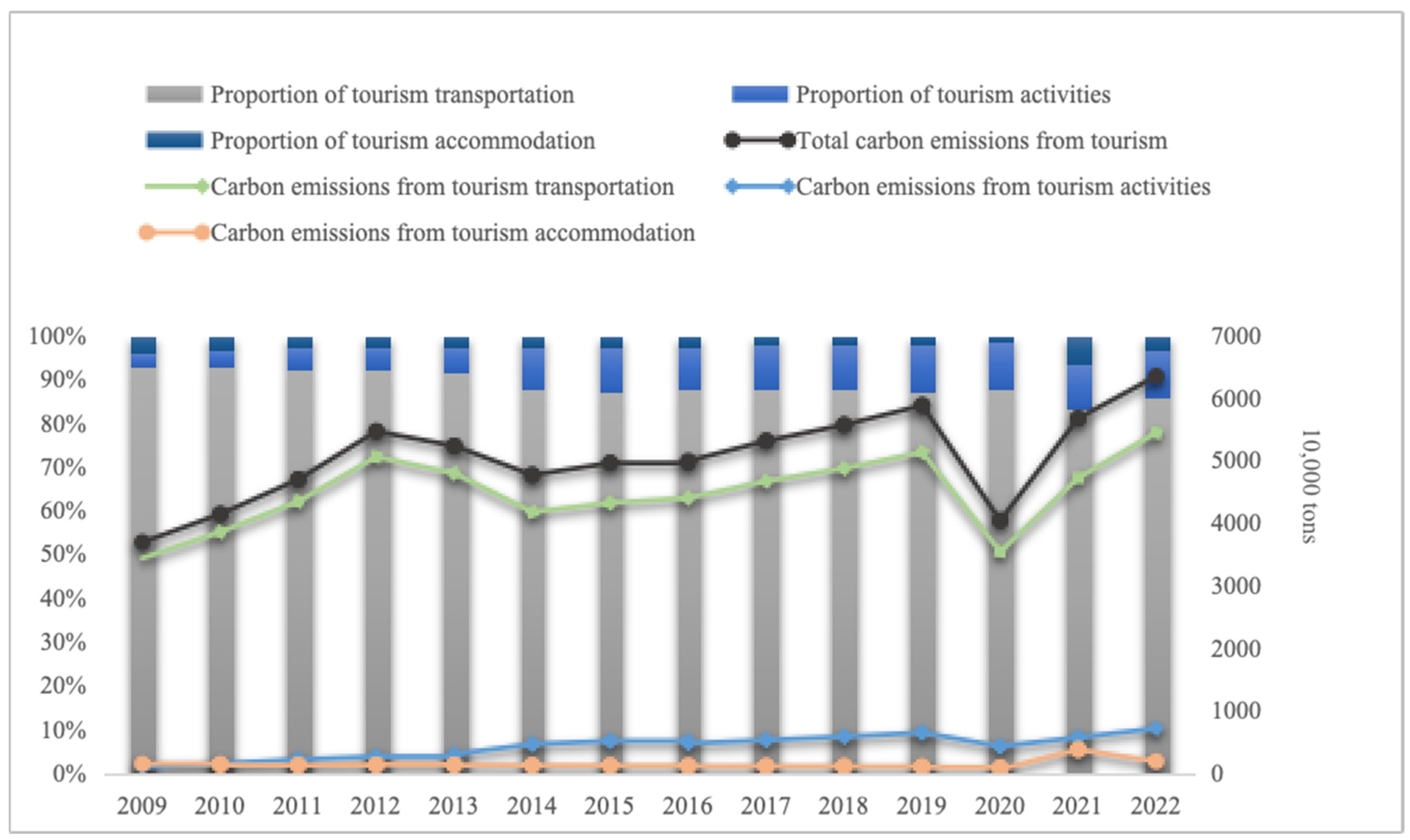
Overall, the carbon emissions show an M-shaped change trend that can be divided into five stages. In the first stage, from 2009 to 2012, tourism carbon emissions slowly increased from 36.88 million tons to 54.64 million tons, with an average annual growth rate as high as 12.09%. In the second stage, from 2012 to 2014, tourism carbon emissions showed a downward trend, dropping to 47.65 million tons, with an average annual growth rate of −4.26%, and the carbon emission level in 2014 was equivalent to that in 2011. In the third stage, from 2014 to 2019, the growth rate of tourism carbon emissions converged, showing an even slower growth. Tourism carbon emissions slowly increased to 58.80 million tons, with an average annual growth rate of 3.90%. In the fourth stage, in 2020, tourism carbon emissions showed a downward trend, and the tourism carbon emissions in the YREB in 2020 were 40.35 million tons. In the last stage, from 2020 to 2022, the tourism industry gradually recovered, and carbon emissions increased rapidly. The tourism carbon emissions in the YREB increased from 36.88 million tons in 2009 to 73.27 million tons in 2019, an increase of 25.71 million tons, with an increase rate as high as 54%. Judging from the annual changes, except for the decreases in 2012 and 2020, the carbon emissions in other years showed an increasing trend. Compared to carbon emissions, the slope of tourism revenue is larger, indicating a decreasing dependence of the tourism industry on energy consumption. This trend may be attributed to the rapid growth of the tourism industry in the Yangtze River Economic Belt during the study period, along with the implementation of various energy-saving and emissions reduction policies after the expansion of the tourism scale. Notably, between 2012 and 2014, there was a significant decrease in carbon emissions from tourism, likely due to the positive impact of pollution reduction policies on the region’s tourism ecological environment. The specific data can be seen in Appendix B 

Table A2. Carbon emissions of the tourism industry in the YREB (2009–2022) (Unit:10,000 tons).

Year	Tourism Transport	Tourism Activities	Tourism Accommodation	Total Carbon Emissions of the Tourism Industry	Total Carbon Emissions of the YREB	Percentage of Carbon Emissions from the Tourism Industry
2009	3433.80	102.38	151.47	3687.65	321,928.08	1.15
2010	3852.99	155.08	130.35	4138.42	348,731.77	1.19
2011	4342.83	221.26	130.28	4694.37	380,425.49	1.23
2012	5055.26	269.04	139.83	5464.14	386,042.90	1.42
2013	4794.03	308.13	129.02	5231.18	385,608.00	1.36
2014	4173.48	466.13	125.52	4765.14	381,938.91	1.25
2015	4317.11	517.36	121.51	4955.98	374,630.53	1.32
2016	4397.98	477.21	115.12	4990.30	379,343.60	1.32
2017	4666.53	530.83	113.53	5310.90	385,323.09	1.38
2018	4872.35	585.88	109.83	5568.07	387,508.19	1.44
2019	5130.30	649.83	99.53	5879.66	398,381.22	1.48
2020	3537.22	432.57	65.72	4035.51	440,609.63	0.92
2021	4719.77	572.95	380.07	5672.80	370,771.24	1.53
2022	5440.80	717.39	190.46	6348.66	391,892.59	1.62

.

In terms of the tourism carbon emission sectors, the proportions of tourism transportation, tourism activities, and tourism accommodation gradually decrease. With the improvement of living standards and the increase in leisure time, tourism demand is stimulated. The proportion of carbon emissions from tourism activities increases, while the proportions of carbon emissions from tourism transportation and tourism accommodation both show a downward trend (Figure 2).

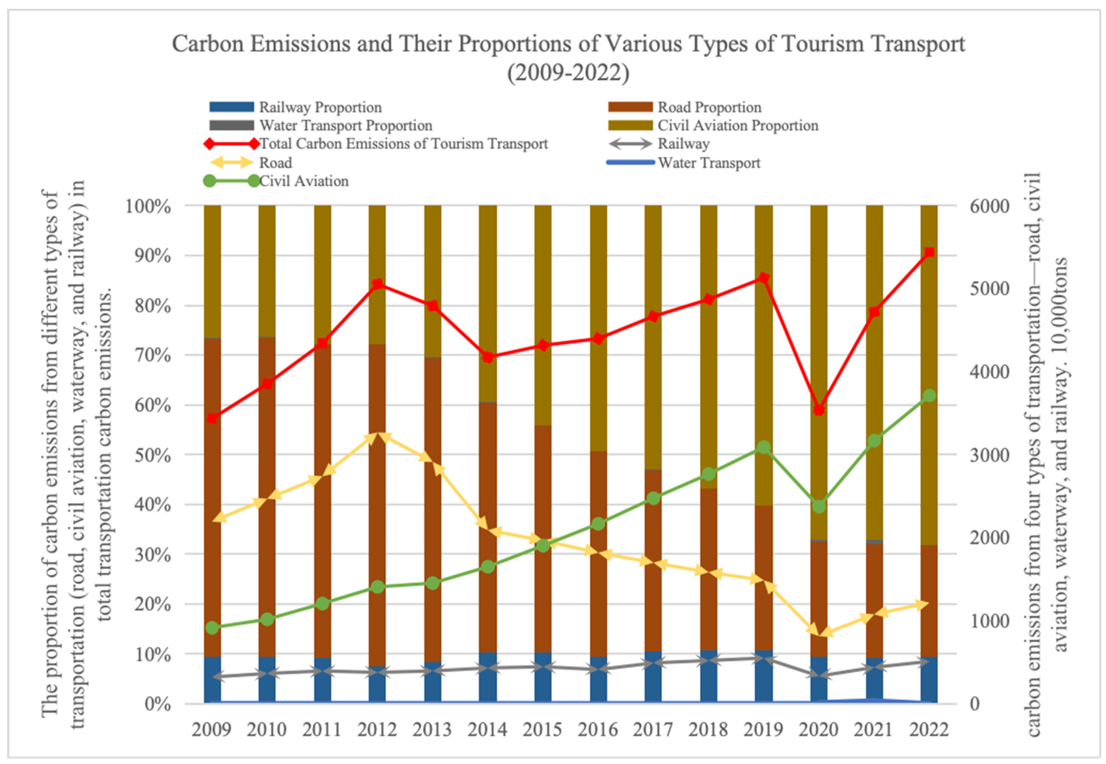
Looking at the changes in the proportion of carbon emissions from various modes of transportation, the carbon emissions from four types of transportation—road, civil aviation, waterway, and railway—in the YREB fluctuated significantly from 2009 to 2022. Road transportation had the highest proportion of carbon emissions, which showed a downward trend; civil aviation ranked second in terms of carbon emissions proportion, which continued to rise; railway ranked third, with little fluctuation in its proportion over the years; and waterway had the lowest proportion of carbon emissions. In terms of the amount of carbon emissions from different types of transportation, the emissions from railway and waterway showed little fluctuation, road transportation emissions decreased, and civil aviation emissions increased. Before 2015, road transportation emissions were higher than those from civil aviation, indicating that road transportation held a central position in the transportation system of the YREB during this period. However, with the improvement of people’s living conditions, changes in consumption concepts, and the completion of high-speed rail construction, tourists had more choices, such as opting for the more time-efficient civil aviation. As a result, in 2015, road transportation emissions began to fall below those of civil aviation (Figure 3).

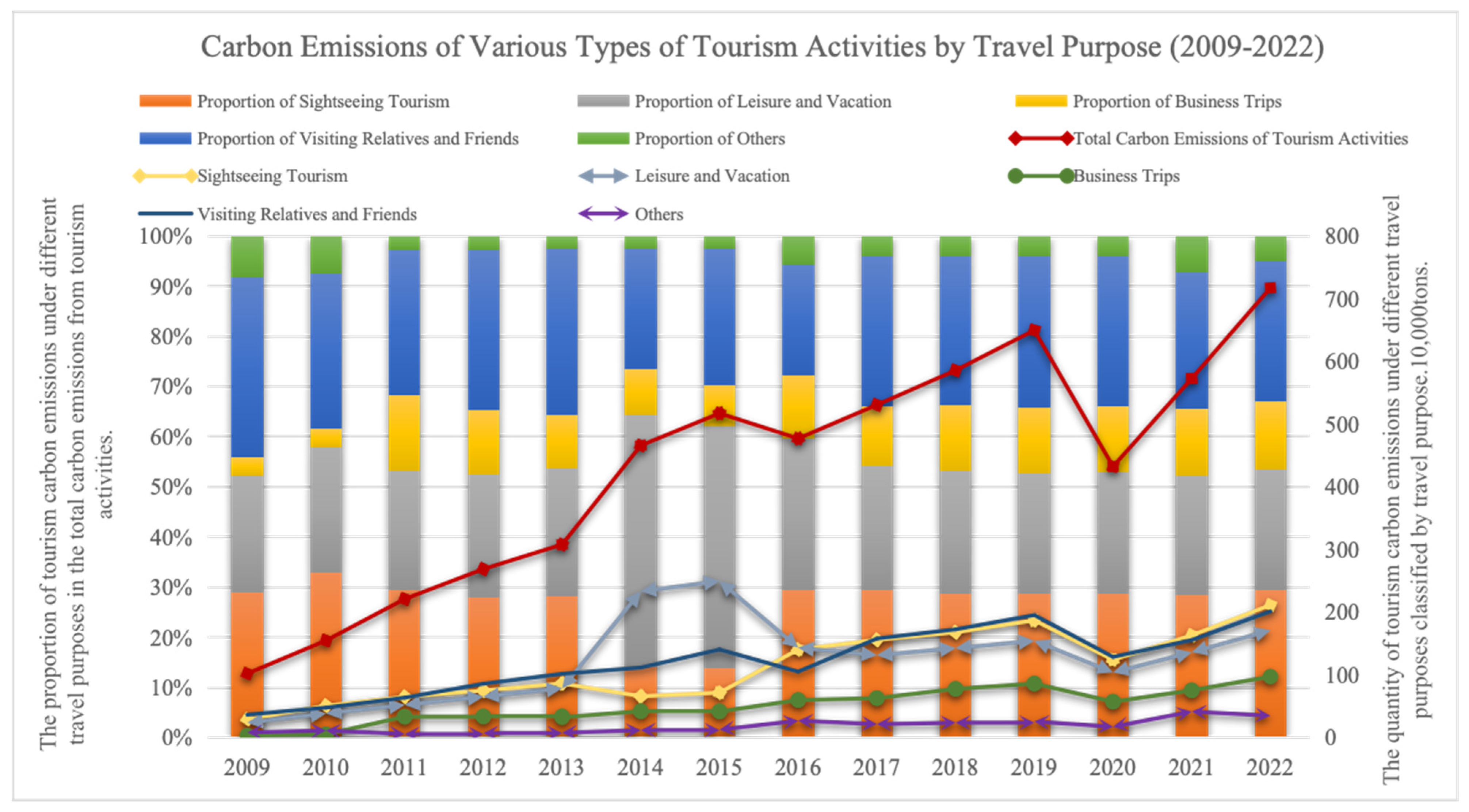
Looking at the carbon emissions of different types of tourism activities divided by travel purposes, apart from leisure and vacation, the carbon emissions of other types of activities generally show an increasing trend year by year. To facilitate a clearer comparison of the carbon emissions of every kind of tourism activity, this study presents a line chart of these five types of tourism activities, as shown in Figure 4. Except for the fluctuating increase and decrease in carbon emissions for leisure and vacation from 2013 to 2016, the carbon emissions of other activities show an increasing trend year by year. The carbon emissions of tourism activities from highest to lowest are leisure and vacation, visiting friends and relatives, sightseeing tourism, business trips, and others. From 2017 to 2022, the carbon emissions from visiting friends and relatives and sightseeing tourism exhibited a similar trend, with comparable quantities, and a notable trend of exceeding the carbon emissions from leisure and vacation activities.

5.1.2. Spatial Correlation

In this study, the GeoDa1.10 software was used to calculate the Moran’s I values of tourism carbon emissions from 2009 to 2022 to test whether there was spatial correlation in the tourism carbon emissions of the YREB. As shown in

Table 2. Values of carbon emissions from the tourism industry in the YREB (2009–2022).

Year	Moran’s I	p-Value	Sd	Z-Value	Mean
2009	−0.0841	0.0010 ***	0.0247	−4.9208	−0.0303
2010	−0.0307	0.0010 ***	0.0191	−2.3263	−0.0307
2011	−0.0659	0.0060 ***	0.0073	4.6964	−0.1002
2012	−0.0452	0.0121 **	0.0245	−2.2835	−0.0302
2013	−0.0302	0.0085 ***	0.0347	−2.8389	−0.0308
2014	−0.0425	0.0032 ***	0.0085	−1.9086	−0.0084
2015	−0.0659	0.0060 ***	0.0073	4.6964	−0.1002
2016	−0.0644	0.0140 **	0.0156	2.3299	−0.1007
2017	−0.1305	0.0670 *	0.0185	−1.7150	−0.0989
2018	−0.0803	0.0900 *	0.0150	1.3100	−0.1000
2019	−0.0550	0.0330 **	0.0176	2.5629	−0.1002
2020	−0.0390	0.0010 ***	0.0125	−3.1931	−0.0302
2021	−0.0905	0.0550 *	0.0285	−1.6150	−0.0889
2022	−0.0421	0.0032 ***	0.0423	−2.3589	−0.0288

Note: ***, **, * indicate that the significance tests have been passed at the 1%, 5%, and 10% levels, respectively.

, the Moran’s I values have passed significance tests at different levels, indicating statistical significance. The spatial distribution of carbon emissions is not entirely random; instead, there is a certain degree of spatial agglomeration and the spatial Matthew effect. During the research period, the Moran’s I values were all negative, and their absolute values were generally small. This indicates that there is spatial negative autocorrelation among the research regions, and the overall spatial heterogeneity is at a medium–low level. That is, there are spatial differences in carbon emission levels among adjacent or nearby provinces and cities. Among them, the absolute value of Moran’s I index in 2017 reached a maximum of 0.1305, indicating that the spatial heterogeneity of tourism carbon emissions in the YREB was the strongest in 2017.

5.1.3. Regional Differences

As shown in

Table 3. Theil index of carbon emissions from the tourism industry in the YREB (2009–2022).

Year	Within the Region						TWR	Contribution Rate within the Region: %	TBR	Contribution Rate Between Regions: %	Theil
	Western		Central		Eastern
	Difference	Contribution Rate: %	Difference	Contribution Rate: %	Difference	Contribution Rate: %
2009	0.0115	21.40	0.0184	34.21	0.0238	44.39	0.0197	31.84	0.0421	68.16	0.0618
2010	0.0033	6.80	0.0194	39.60	0.0262	53.60	0.0192	35.92	0.0342	64.08	0.0534
2011	0.0122	22.06	0.0091	16.38	0.0343	61.56	0.0222	49.10	0.0231	50.90	0.0453
2012	0.0574	65.25	0.0089	10.09	0.0217	24.65	0.0276	46.27	0.0320	53.73	0.0597
2013	0.0182	12.99	0.0150	10.72	0.1071	76.30	0.0557	61.88	0.0343	38.12	0.0899
2014	0.0199	12.36	0.0141	8.72	0.1276	78.92	0.0624	92.50	0.0051	7.50	0.0674
2015	0.0277	12.81	0.0114	5.25	0.1774	81.94	0.0805	98.34	0.0014	1.66	0.0819
2016	0.0458	15.80	0.0248	8.56	0.2194	75.64	0.1016	95.96	0.0043	4.04	0.1059
2017	0.0698	21.75	0.0085	2.64	0.2426	75.60	0.1067	89.71	0.0122	10.29	0.1189
2018	0.0836	23.09	0.0086	2.38	0.2699	74.53	0.1166	84.46	0.0214	15.54	0.1380
2019	0.0965	23.88	0.0108	2.68	0.2967	73.43	0.1259	78.88	0.0337	21.12	0.1597
2020	0.2753	48.29	0.0770	13.51	0.2179	38.21	0.1863	88.76	0.0236	11.24	0.2099
2021	0.0122	22.06	0.0091	16.38	0.0343	61.56	0.0222	49.10	0.0231	50.90	0.0453
2022	0.0172	12.88	0.0176	10.83	0.1071	76.30	0.0557	61.88	0.0343	38.12	0.0899

, the Theil index of inter-regional and intra-regional differences both show a fluctuating upward trend. The inter-regional difference decreased from 0.0421 in 2009 to 0.0343 in 2022, while the intra-regional difference increased from 0.0197 in 2009 to 0.0557 in 2022. From 2014 to 2015, the Theil index of carbon emission differences among the western, central, and eastern regions increased. From 2016 to 2018, the intra-regional Theil index decreased, and from 2018 to 2022, the Theil index of the east region remained relatively stable. By analyzing the regional contribution rates (as shown in Table 3), we found that the main reason for the regional differences in carbon emissions was the intra-regional difference, with an average contribution rate of 71.14%. In comparison, the average inter-regional contribution rate was only 28.86%.

The population density, social environment, and tourism development conditions in the central and western regions are relatively similar, but there are significant differences compared to the more developed eastern region. From 2014 to 2015, the Theil index of carbon emission differences in the western, central, and eastern areas all increased, which is primarily related to the differing foundations of emission reduction technologies in these regions. Between 2016 and 2018, the Theil index for intra-regional differences decreased, as the improvement of energy-saving and emission-reduction technologies in the central and western regions was relatively faster compared to the high carbon emissions from tourism in the eastern region, thereby narrowing the regional differences in tourism carbon emissions. From 2018 to 2022, the Theil index in the east of the region remained relatively stable, while the index in the central and western regions increased, indicating that the differences in carbon emissions from tourism within these regions had widened. This may be due to the diminishing marginal returns of carbon reduction between provinces, leading to a slowdown in growth, along with the differing foundations of tourism development and policies, which have increased the disparity. The reliance on intra-regional differences in the formation of regional inequality in tourism carbon emissions has weakened. However, the contribution rate of intra-regional differences remains above 50%, indicating the need to reduce these differences further and continue promoting coordinated ecological governance of the Yangtze River International Golden Tourism Belt.

5.2. Temporal and Spatial Evolution of Decoupling Status

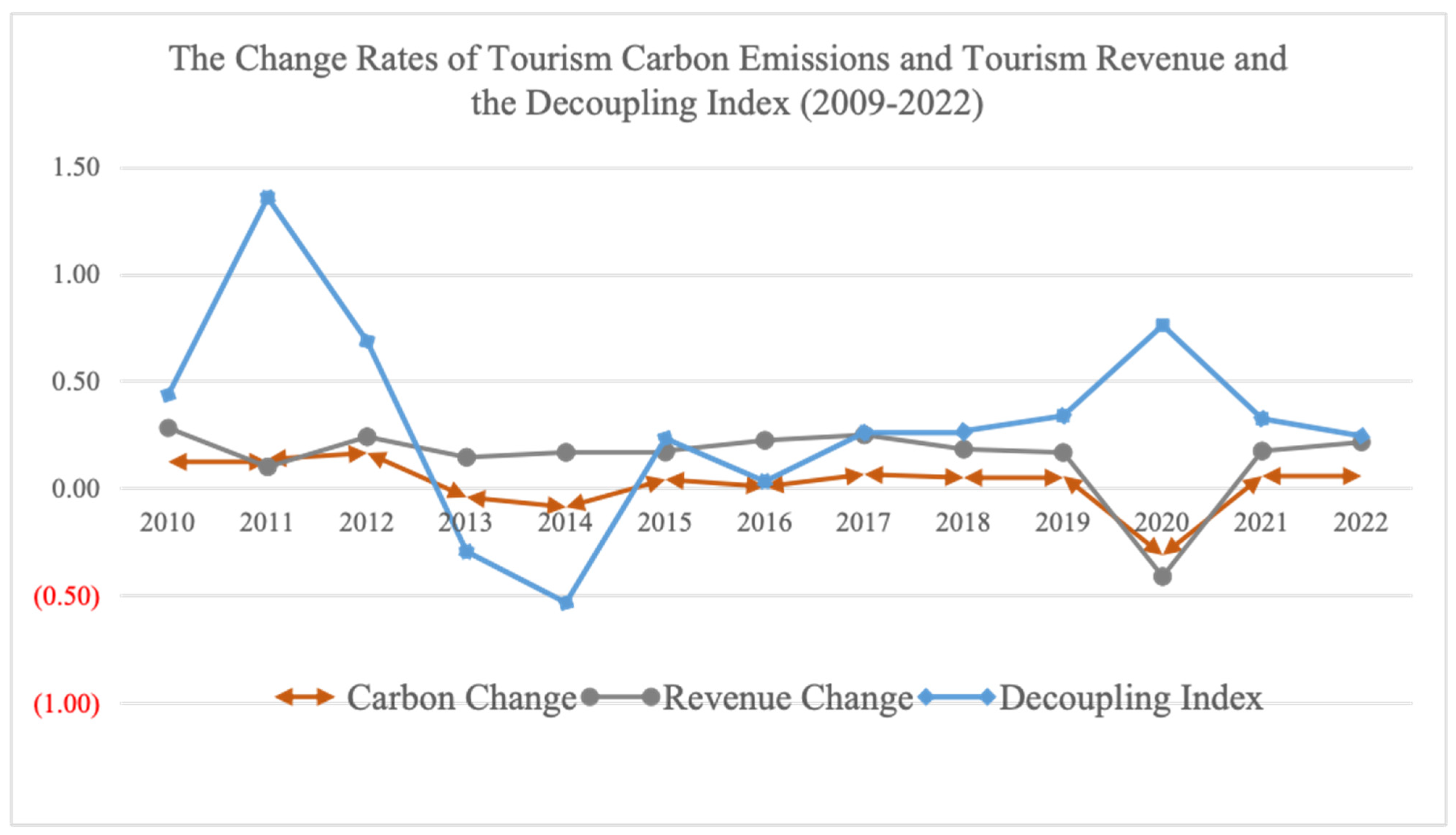
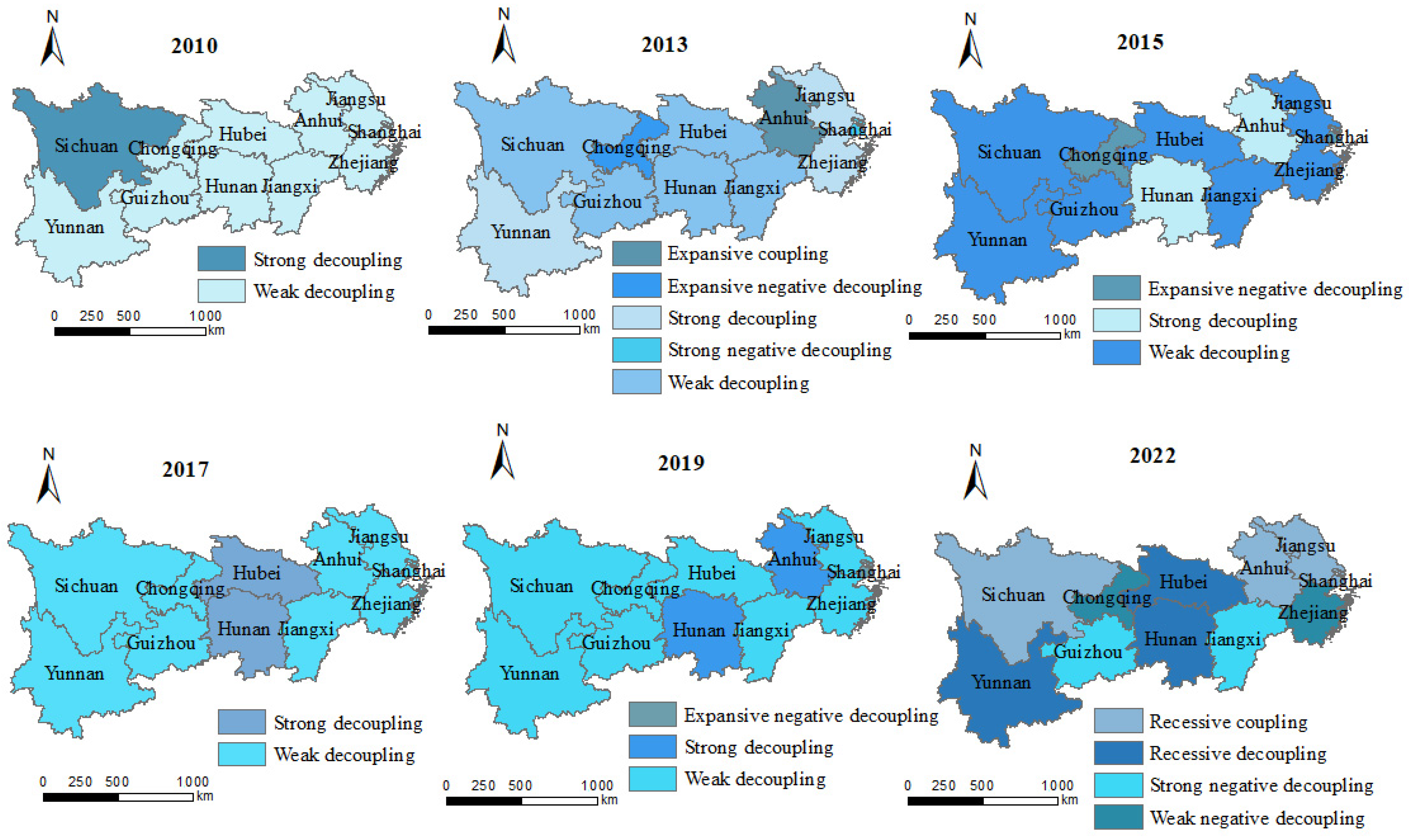
Based on the Tapio model, this study analyzes the decoupling relationship between the tourism economy and tourism carbon emissions in the YREB. During the research period, three types of decoupling states were presented: weak decoupling, expansive negative decoupling, and strong decoupling, finally stabilizing at weak decoupling with an average decoupling index of 0.277. Except for the year 2011, which showed expansive negative decoupling, the decoupling state from 2010 to 2022 was relatively optimistic. However, the fact that the decoupling state has remained stable at weak decoupling for many years also indirectly reflects the need to adopt effective technologies to optimize the decoupling state towards strong decoupling (Figure 5).

This study used ArcGIS10.8 software to achieve spatial visualization and analyzed the spatial evolution characteristics of tourism carbon decoupling over the years. The fact that most regions are in a stable state of weak decoupling indicates the necessity to systematically monitor and plan the carbon emissions of key tourism industries and related industries in these provinces to regulate the decoupling state and level of tourism carbon emissions and to promote a transition towards a strong decoupling state. Drawing on the experience of developed countries, decoupling generally goes through a process of strong decoupling–weak decoupling–negative decoupling–strong decoupling. The YREB still has a long way to go to follow this trend. Therefore, to achieve truly low-carbon tourism development, it is necessary to re-examine the industries related to tourism from a holistic and systematic perspective and to monitor the decoupling stage of tourism economic growth and tourism carbon emissions in the entire industry chain of tourism development (Figure 6).

5.3. Driving Factors of Decoupling Tourism Carbon

The GWR results show that during the research period, eight driving factors affecting the decoupling of tourism carbon in the YREB have mostly passed the significance test and are statistically significant. The significant driving factors are urbanization level (UI), industrial structure (IS), government policy (GP), technological innovation capability (TIC), regional economic strength (RGDP), and consumption level (CL). However, consumer spending power (CSP) and tourist scale (TA) are not driving factors. Given the characteristic of the GWR model being suitable for cross-sectional data, this study selects the average values of the indicators of each influencing factor in six years—2010, 2013, 2015, 2017, 2019, and 2022—during the period from 2010 to 2022. The range normalization method was used to eliminate the dimension, and ArcGIS software was employed for GWR spatial modeling regression.

5.3.1. Cross-Sectional Heterogeneity Analysis

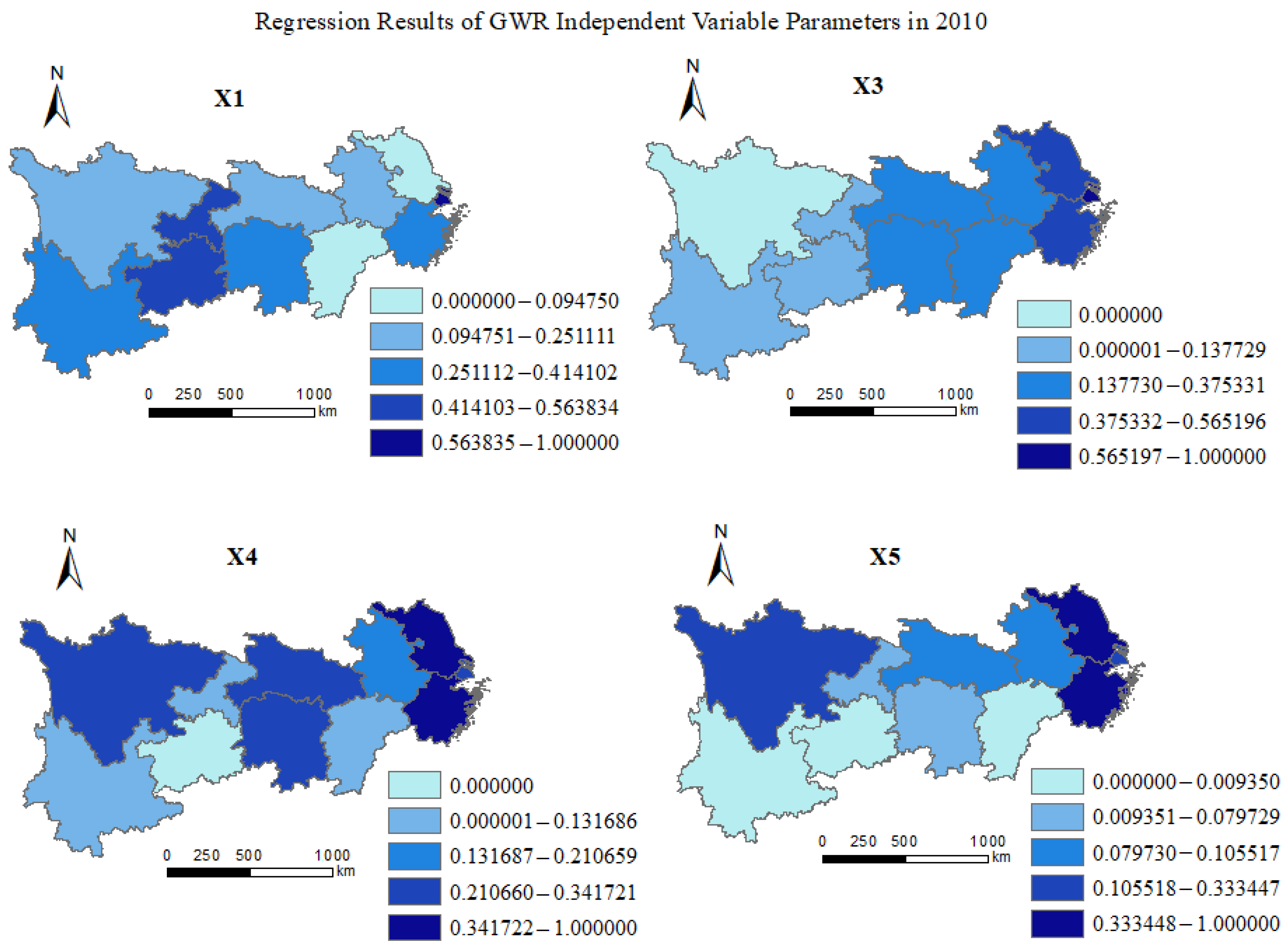
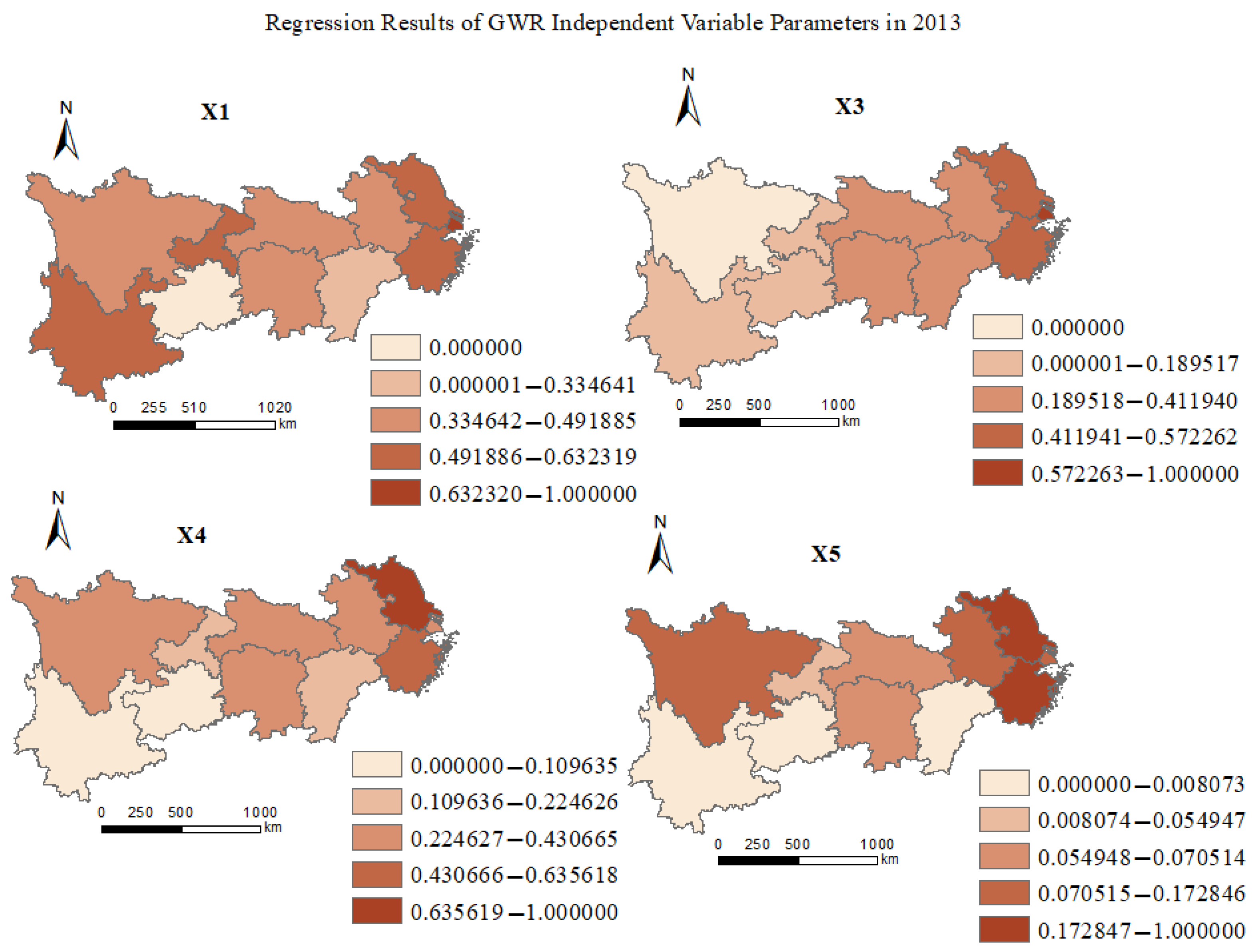
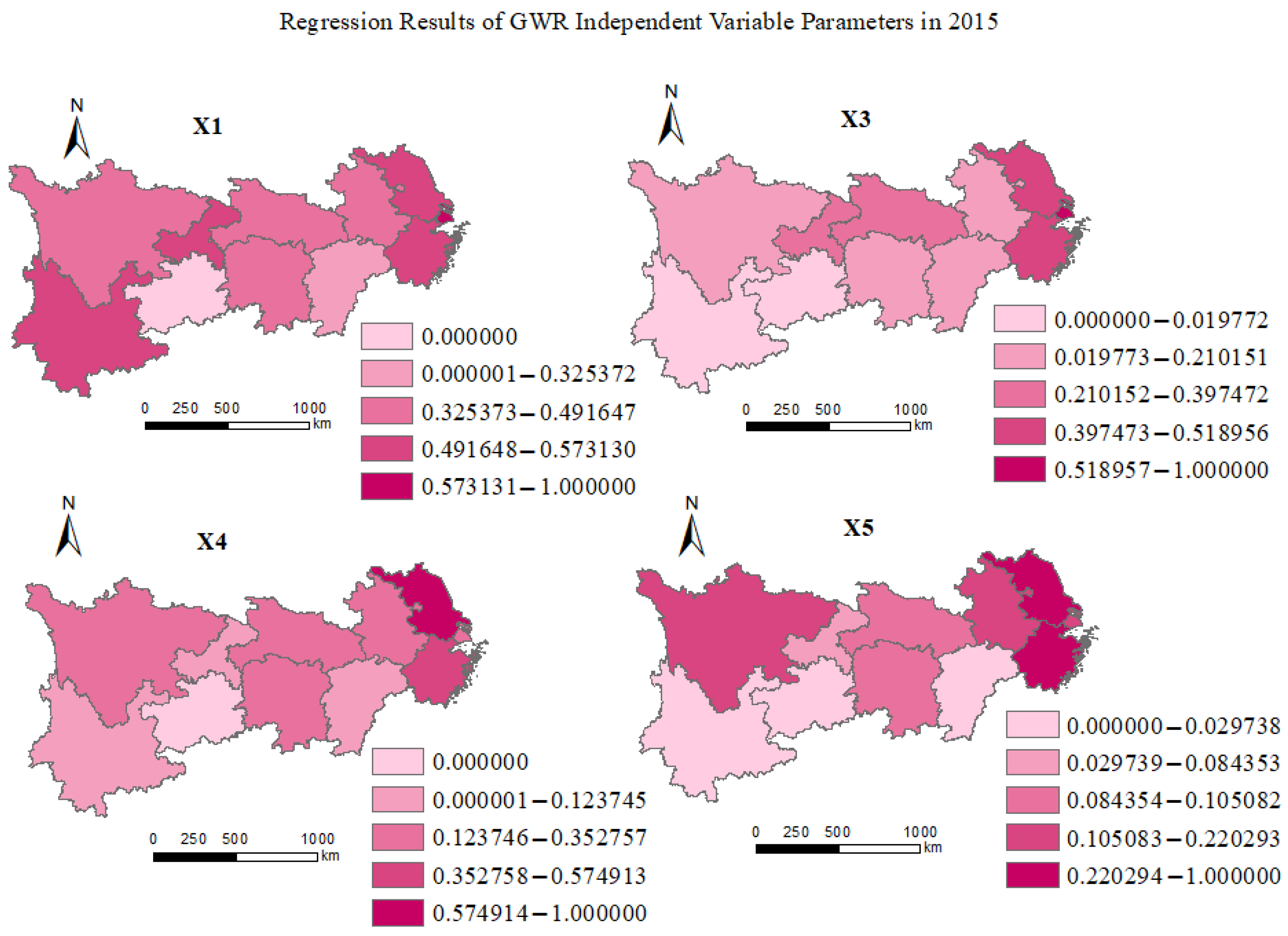
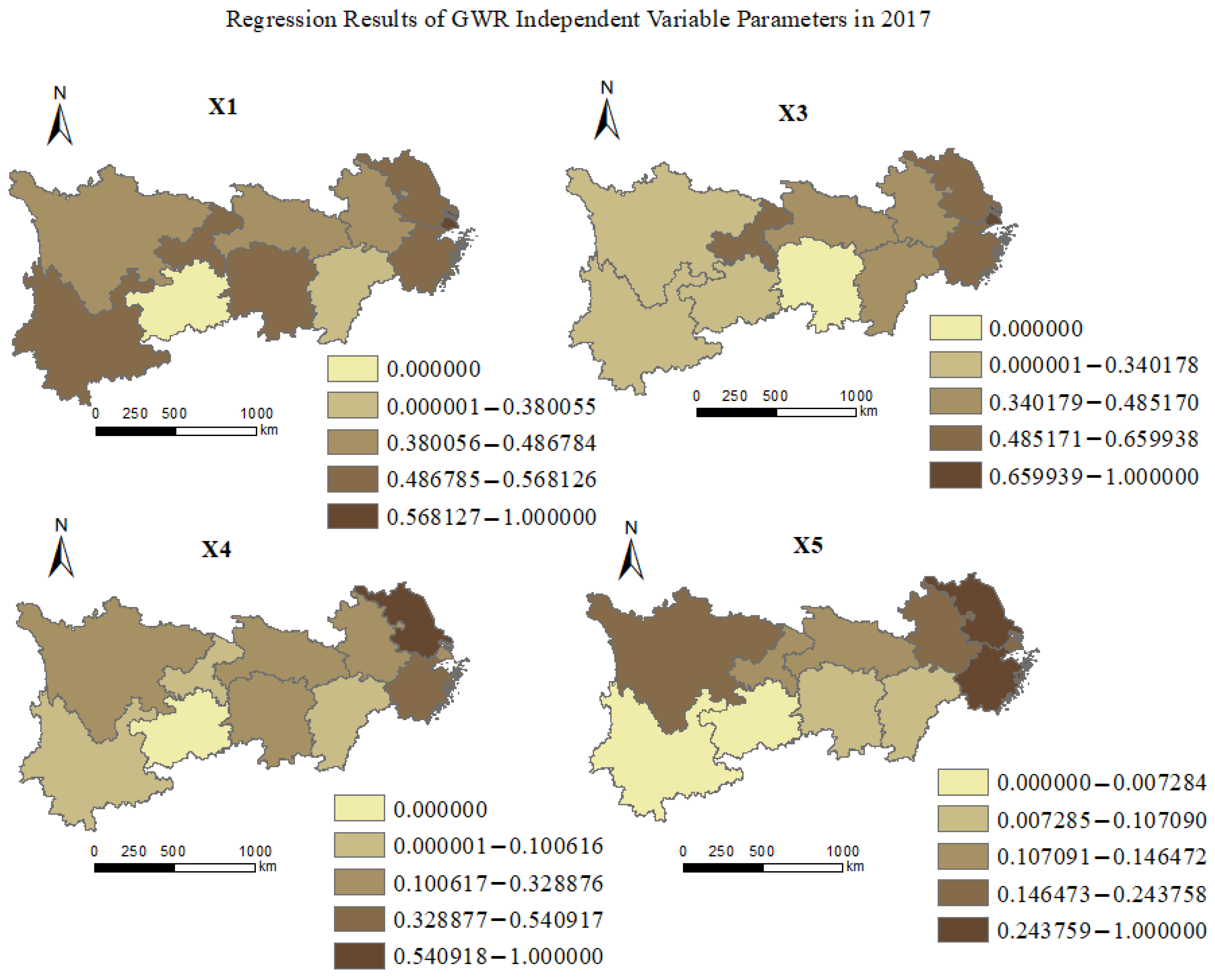
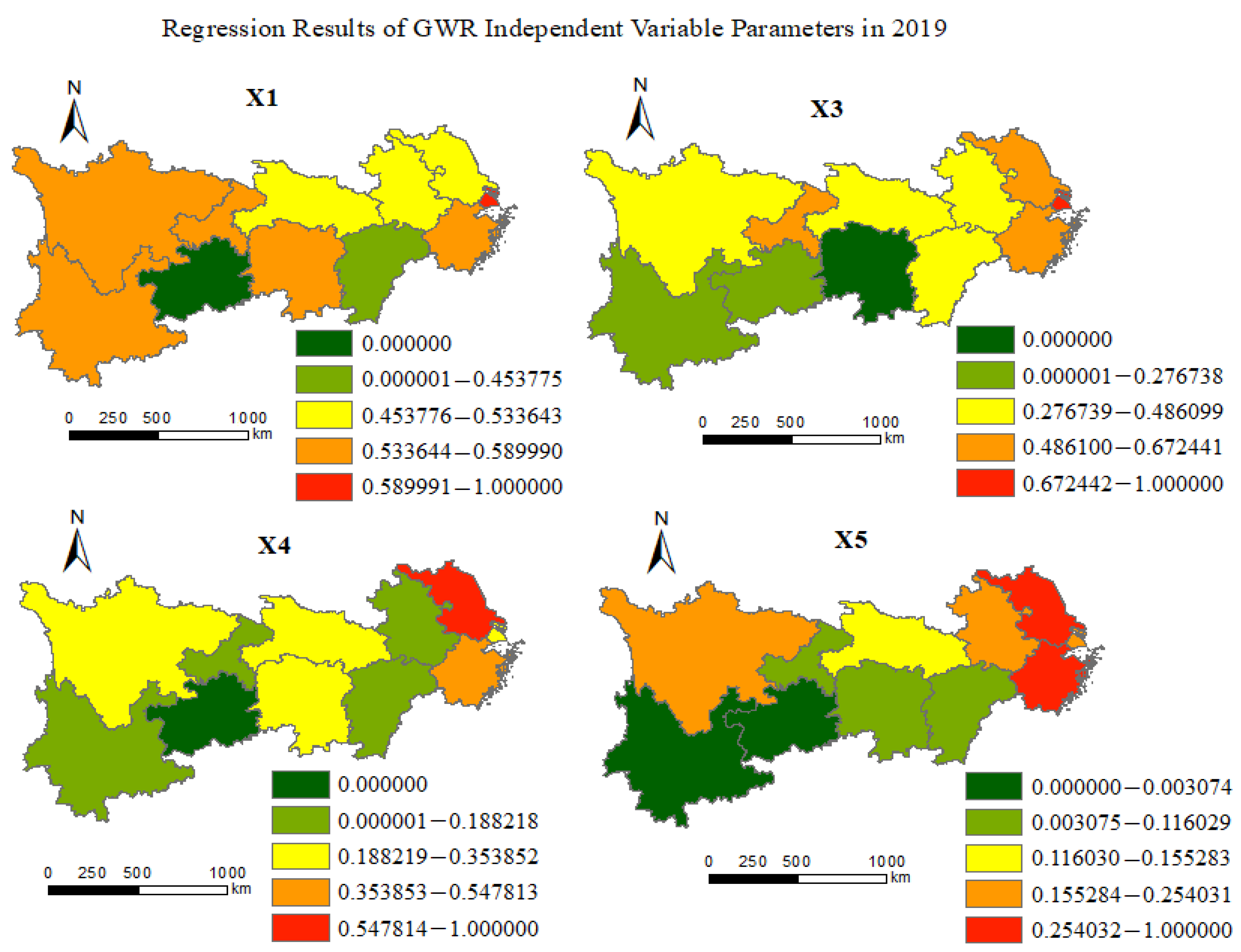
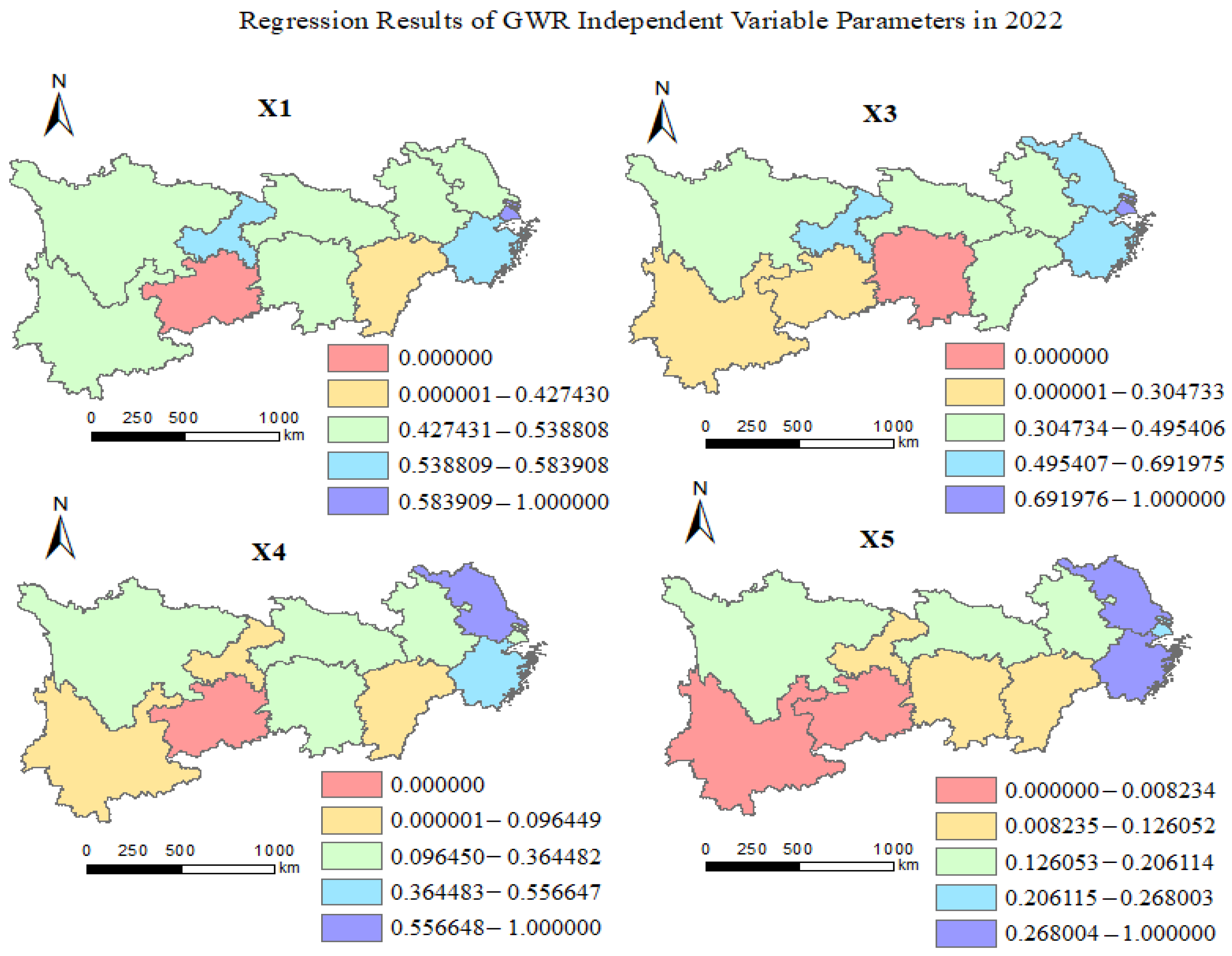
Using the GWR model can yield a set of regression coefficients for each region. As can be seen from the spatial distribution of the regression coefficients shown in Figure 7, Figure 8, Figure 9, Figure 10, Figure 11 and Figure 12, there is spatial heterogeneity in the evolution of the decoupling state of tourism carbon in the YREB. Looking at the cross-sectional data regression results for different years, there is a significant difference in the numerical range of the regression coefficients of the independent variables, indicating that there are also differences in the impact effects of regional tourism carbon decoupling.

The GWR results for 2010 show that the impact effect of industrial structure (X1) on tourism carbon decoupling in each provincial region is significantly adverse, the impact effect of urbanization level (X3) is significantly positive, the scale effect of regional economic strength (X4) is significantly adverse, and the impact effect of technological innovation capability (X5) is positive, but the absolute value of the coefficient is less than that of the urbanization level coefficient; that is, the positive effect generated by technological innovation capability is not higher than the urbanization level.

The GWR results for 2013 show that the scale effect of regional economic strength (X4) in each provincial region remains significantly negative, and the impact effect of technological innovation capability (X5) remains positive, but its impact effect on decoupling is enhanced (the absolute value of the coefficient increases).

The GWR results for 2015 show that the impact effects of industrial structure (X1), urbanization level (X3), regional economic strength (X4), and technological innovation capability (X5) on tourism carbon decoupling in each provincial region have changed little compared with 2013.

The GWR results for 2017 show that the impact effect of industrial structure (X1) on tourism carbon decoupling in each provincial region is significantly positive, the impact effect of urbanization level (X3) is significantly positive, the scale effect of regional economic strength (X4) is significantly positive, and the impact effect of technological innovation capability (X5) is negative.

The GWR results for 2019 show that the impact directions of industrial structure (X1), urbanization level (X3), regional economic strength (X4), and technological innovation capability (X5) on tourism carbon decoupling in each provincial region are consistent with those in 2017, but the impact effects have a trend of increasing.

The GWR results for 2022 show that, except for urbanization level (X3), the impact directions of industrial structure (X1), regional economic strength (X4), and technological innovation capability (X5) on tourism carbon decoupling in each provincial region are consistent with those in 2019, and the impact effects have a trend of increasing.

5.3.2. Provincial Spatial-Temporal Heterogeneity Analysis

Combining the empirical results of GWR, based on the descriptive statistics of the GWR estimated parameters for the 11 provinces and cities from 2010 to 2022 (as shown in

Table 4. Descriptive statistics of parameter estimates for each independent variable from 2010 to 2022.

Core Parameter	Maximum Value	Minimum Value	Mean	Median
β1	3.02	0.22	1.44	0.31
β2	1.09	−3.41	−1.11	−1.97
β3	3.48	−8.75	−2.19	−0.88
β4	6.43	−2.52	1.38	0.91

), it can be seen from the maximum and minimum values that there is a large spatial variability in the explanatory variables. The median and mean are relatively close, indicating that the impact nature of this regression tends to be the same within the spatial scope. Based on the regression coefficient results of the GWR model, this study uses the natural breakpoint method of ArcGIS to visually express it in space and further delineate the spatial differences of the regression coefficients of each influencing factor.

(i)

Spatial-Temporal Heterogeneity of Industrial Structure Impact

From 2010 to 2022, the industrial structure (X1) of the 11 provinces and cities had a positive impact on tourism carbon decoupling. The differences in regional regression coefficients were relatively significant, with the coefficient gap fluctuating between −0.22 and 3.02. This indicates that there is significant spatial heterogeneity in the industrial structure of the 11 provinces and cities, and the differences in industrial structure and its environmental effects vary across different regions. From 2010 to 2014, the regions with a strong impact effect of industrial structure (X1) shifted from the western to the central regions. From 2014 to 2022, the impact effect of industrial structure showed a decreasing trend but remained positive. Overall, it can be seen that the industrial structure (X1) plays an important role in promoting tourism carbon decoupling in the YREB region.

(ii)

Spatial-Temporal Heterogeneity of Urbanization Level Impact

From 2010 to 2014, the urbanization level (X3) of the region had a negative impact on tourism carbon decoupling, with minimal fluctuations in the differences in regional regression coefficients, and the coefficient gap was basically maintained at around 0.02. This indicates that the spatial dependence of the region’s urbanization level on tourism carbon decoupling has not changed significantly. In 2016, the impact effect of urbanization level (X3) on tourism carbon decoupling was positive, but it was negative in 2018 and 2022. It is possible that different levels of urbanization have different impacts on tourism carbon decoupling in different regions. Excessive urbanization and rapid development of urban tourism may lead to an overly rapid increase in tourism carbon emissions [30], which is not conducive to tourism carbon decoupling.

(iii)

Spatial-Temporal Heterogeneity of Regional Economic Strength Impact

From 2010 to 2016, regional economic strength (X4) had a negative impact on tourism carbon decoupling. The differences in regression coefficients across regions first increased and then decreased, with the coefficient gap expanding from 0.006 to 0.044 and then narrowing to 0.002. This indicates that the spatial dependence of regional GDP production scale on tourism carbon decoupling first decreased and then increased, and the differences in economic scale effects and their environmental impacts first increased and then decreased. From 2016 to 2018, the impact of regional economic strength (X4) on regional tourism carbon decoupling increased, with the average regression coefficient rising from 0.51 in 2016 to 1.19 in 2018 and then to 3.48 in 2022. Overall, the boosting effect of regional economic strength on tourism carbon decoupling has generally increased, but the differences it brings to the regions are being reduced.

(iv)

Spatial-Temporal Heterogeneity of Technological Innovation Capability Impact

From 2010 to 2016, the impact of technological innovation capability (X5) on tourism carbon decoupling changed from positive to negative, indicating that the spatial dependence of regional technological innovation capability on tourism carbon decoupling has not been exacerbated. From 2016 to 2022, the impact effect of technological innovation capability has been negative, which may be due to the high costs of technological innovation in the early stage, while the benefits have not yet been highlighted. As shown in

Table 5. Average values of estimated parameters for each independent variable from 2010 to 2022.

Year	X1	X3	X4	X5
2010	−0.22	0.69	−0.89	0.36
2012	0.31	3.41	−1.78	5.49
2014	0.33	3.45	−1.23	4.43
2016	0.13	1.09	0.51	−0.91
2018	0.31	0.40	1.19	−1.51
2020	1.35	−0.53	2.56	−1.87
2022	2.41	−1.97	3.78	−2.52

, the average regression coefficient changed from 0.36 in 2010 to −0.91 in 2016, and then to −2.52 in 2022. The increase in the absolute value of the regression coefficient indicates that the impact effect of technological innovation on tourism carbon decoupling has also been enhanced.

6. Discussion

6.1. Theoretical Contributions

Deepening the theoretical understanding of tourism carbon decoupling, this study systematically combs through the theories related to tourism carbon emission estimation and carbon decoupling, enriching the theoretical research on the relationship between tourism economy and environment. In terms of tourism carbon emission estimation, it summarizes various methods such as the carbon footprint method, input–output method, top-down approach, and bottom-up approach [6,25,26,27]; clarifies the basic ideas, characteristics, research scales, and applicable scopes of each method; and provides a comprehensive theoretical reference for future studies in selecting estimation methods. This helps to more accurately estimate tourism carbon emissions and deepen the understanding of the carbon emission mechanisms of tourism activities.

Expanding the application scope of decoupling theory, this study applies decoupling theory to the tourism industry, thoroughly analyzing the decoupling relationship between tourism economic growth and carbon emissions. Drawing on the decoupling index proposed by Tapio (2005) [28], it clarifies that there are multiple decoupling states in the tourism economic system of the YREB and analyzes their spatiotemporal evolution characteristics. Unlike previous studies that mostly focused on the national scale or used provinces, cities, or tourist attractions as units [28], this study focuses on the YREB, a meso-macro region, providing a new empirical case for the application of decoupling theory in regional tourism development research, expanding the scope of application of this theory, and promoting the development of decoupling theory in the tourism field.

By integrating the GWR model with the Tapio decoupling model, this study explores the driving factors and interactive effects of the decoupling relationship between tourism economy and tourism carbon emissions, making up for the shortcomings in existing research [10,23,24]. It identifies significant driving factors such as urbanization level, industrial structure, government policy, technological innovation capability, regional economic strength, and consumption level, and analyzes the differences in the direction and degree of their impact on tourism carbon decoupling in different years and provincial regions. This not only deepens the understanding of the complex relationship between tourism economy and carbon emissions but also provides important support for building a more comprehensive theoretical framework for sustainable tourism development. It also offers new research ideas and methods for future studies exploring the relationship between regional tourism development and carbon emissions.

6.2. Policy Implications

To promote the orderly low-carbon transformation and upgrading of the tourism industry, the development of the tourism industry in the YREB must continue to unswervingly implement the new development philosophy, adjust the economic structure of the tourism industry, and integrate the concept of prioritizing ecology and green development into all aspects of innovation-driven tourism industry. This means upgrading and continuously promoting the realization of the “Dual Carbon” goals and high-quality development of the tourism industry.

Eastern regions should take on more emission reduction responsibilities. Provinces with different emission reduction statuses may have different emission reduction potentials. The planning of emission reduction pathways should take into account both emission reduction capabilities and barriers. The eastern regions have higher historical emissions and need to take on more emission reduction responsibilities. At the same time, the decoupling status of the eastern regions is not satisfactory, and it is necessary to focus on finding ways to break the path dependence of tourism development on high-carbon emissions, explore new low-carbon tourism models, strengthen carbon emission monitoring of various tourism activities, clarify the carbon emission responsibilities of relevant actors, formulate low-carbon behavior guidelines, and establish reward and punishment mechanisms. The focus should be on technological and institutional innovation to further achieve low-carbon growth in tourism development.

Coordinated regional development should be promoted and efforts should be made to reduce spatial differences in tourism carbon emissions and form good tourism industry agglomeration effects. At the same time, the radiating and driving role of good decoupling trends in the region should be strengthened. Administrative regional restrictions should be broken to promote green and low-carbon cooperation among provinces and cities within the region, and coordinated low-carbon integrated development of the tourism industry should be promoted. A carbon reduction spatial pattern for tourism development that matches the development positioning and is complementary in the region should be formed to support the construction of green demonstration zones.

6.3. Limitations and Future Directions

This study has limitations. First, the estimation of tourism carbon emissions still has errors. For example, in the estimation of carbon emissions from tourism accommodation, due to the lack of data, this study only includes star-rated hotels. Second, in terms of research scale, due to the poor availability of data, this study can only be conducted at the provincial level. More micro-level research may be a key direction for future studies. Third, although the GWR model can more accurately depict the way, direction, path, and intensity of the effects of each driving factor, the impact of the same factor may vary depending on its scope of influence and cannot be generalized. The complexity of regional economic phenomena and the interactive and superimposed effects among influencing factors may also lead to errors in the interpretation of the mechanisms of influence. Future research can focus on more micro-level studies, and improving the accuracy of carbon emission estimation will also be a key research direction in the future.

7. Conclusions

This study has conducted an in-depth investigation into the spatiotemporal evolution and driving forces of tourism carbon decoupling in the YREB. In terms of tourism carbon emissions, the emissions show an M-shaped trend, with a significant increase from 2009 to 2022. The proportions of carbon emissions from tourism transportation, activities, and accommodation have changed, and the proportions of carbon emissions from road and civil aviation in transportation have shown significant fluctuations. Spatially, there is heterogeneity and negative autocorrelation in carbon emissions, with inter-regional differences narrowing and intra-regional differences increasing. Intra-regional differences are the main cause of overall differences. Looking at the decoupling status, the tourism economic system of the YREB has experienced weak decoupling, expansive negative decoupling, and strong decoupling, and finally stabilized at weak decoupling. Regionally, the western and eastern regions are more consistent with the overall decoupling trend. Although the eastern region shows an improving trend, it still needs to explore new models of low-carbon development. Some provinces have a better decoupling status, while Shanghai, Zhejiang, and other places have larger fluctuations. Regarding the driving factors affecting decoupling, most factors, such as urbanization level and industrial structure, have passed the significance test. These factors show spatial heterogeneity, and the direction and degree of their impact on tourism carbon decoupling in each provincial region vary in different years. In addition, the estimation of carbon emissions from tourism still carries errors. For example, in estimating carbon emissions from tourism accommodation, the study is limited to star-rated hotels due to a lack of data. In terms of research scale, the study can only be conducted at the provincial level because of data accessibility issues; more micro-level studies may become a key research direction in the future. Finally, the complexity of regional economic phenomena and the interaction effects among influencing factors may also lead to inaccuracies in understanding the underlying mechanisms. Therefore, accurately estimating carbon emissions from tourism and further analyzing the driving mechanisms of tourism carbon decoupling at different scales will be important research directions moving forward.

References

1. Zhu, Y.; Hu, Y.; Zhu, Y. Can China’s energy policies achieve the “dual carbon” goal? A multi-dimensional analysis based on policy text tools. Environ. Dev. Sustain. 2024, 1–40. [Google Scholar] [CrossRef]
2. Zhou, M.; Yang, J.; Ning, X.; Wu, C.; Zhang, Y. Analysis of the Characteristics and Driving Mechanisms of Carbon Emission Decoupling in the Hu-Bao-O-Yu City Cluster under the “Double Carbon” Target. Sustainability 2024, 16, 7290. [Google Scholar] [CrossRef]
3. Chen, H.; Peng, X.; Wang, Z.; Bo, Y. Research on Decoupling Relationship among Energy Consumption, Carbon Emissions, and Economic Growth under Dual Carbon Goals in China. In Proceedings of the 2023 3rd Power System and Green Energy Conference (PSGEC), Shanghai, China, 24–26 August 2023; IEEE: New York, NY, USA, 2023; pp. 779–784. [Google Scholar]
4. Gössling, S. Carbon neutral destinations: A conceptual analysis. J. Sustain. Tour. 2009, 17, 17–37. [Google Scholar] [CrossRef]
5. Eika, L.; Mogstad, M.; Vestad, O.L. What can we learn about household consumption expenditure from data on income and assets? J. Public Econ. 2020, 189, 104163. [Google Scholar] [CrossRef]
6. Lenzen, M.; Sun, Y.Y.; Faturay, F.; Ting, Y.P.; Geschke, A.; Malik, A. The carbon footprint of global tourism. Nat. Clim. Change 2018, 8, 522–528. [Google Scholar] [CrossRef]
7. Reilly, J.; Williams, P.; Haider, W. Moving towards more eco-efficient tourist transportation to a resort destination: The case of Whistler, British Columbia. Res. Transp. Econ. 2010, 26, 66–73. [Google Scholar] [CrossRef]
8. Gössling, S.; Peeters, P. Assessing tourism’s global environmental impact 1900–2050. J. Sustain. Tour. 2015, 23, 639–659. [Google Scholar] [CrossRef]
9. Zhang, J.; Zhang, Y. Carbon tax, tourism CO2 emissions and economic welfare. Ann. Tour. Res. 2018, 69, 18–30. [Google Scholar] [CrossRef]
10. Zha, J.; Dai, J.; Ma, S.; Chen, Y.; Wang, X. How to decouple tourism growth from carbon emissions? A case study of Chengdu, China. Tour. Manag. Perspect. 2021, 39, 100849. [Google Scholar] [CrossRef]
11. Tang, Z.; Shang, J.; Shi, C.; Liu, Z.; Bi, K. Decoupling indicators of CO2 emissions from the tourism industry in China: 1990–2012. Ecol. Indic. 2014, 46, 390–397. [Google Scholar] [CrossRef]
12. Karakaya, E.; Bostan, A.; Özçağ, M. Decomposition and decoupling analysis of energy-related carbon emissions in Turkey. Environ. Sci. Pollut. Res. 2019, 26, 32080–32091. [Google Scholar] [CrossRef]
13. Climent, F.; Pardo, A. Decoupling factors on the energy–output linkage: The Spanish case. Energy Policy 2007, 35, 522–528. [Google Scholar] [CrossRef]
14. Robaina-Alves, M.; Moutinho, V.; Costa, R. Change in energy-related CO2 (carbon dioxide) emissions in Portuguese tourism: A decomposition analysis from 2000 to 2008. J. Clean. Prod. 2016, 111, 520–528. [Google Scholar] [CrossRef]
15. Tang, C.; Zhong, L.; Ng, P. Factors that influence the tourism industry’s carbon emissions: A tourism area life cycle model perspective. Energy Policy 2017, 109, 704–718. [Google Scholar] [CrossRef]
16. Chen, J.; Zhao, A.; Zhao, Q.; Song, M.; Baležentis, T.; Streimikiene, D. Estimation and factor decomposition of carbon emissions in China’s tourism sector. Probl. Ekorozwoju 2018, 13, 91–101. [Google Scholar]
17. Li, L.; Li, J.; Tang, L.; Wang, S. Balancing tourism’s economic benefit and CO2 emissions: An insight from input–output and tourism satellite account analysis. Sustainability 2019, 11, 1052. [Google Scholar] [CrossRef]
18. Ma, H.; Liu, J.; Xi, J. Decoupling and decomposition analysis of carbon emissions in Beijing’s tourism traffic. Environ. Dev. Sustain. 2022, 24, 5258–5274. [Google Scholar] [CrossRef]
19. Xie, P.; Gao, S.; Sun, F. An analysis of the decoupling relationship between CO2 emission in power industry and GDP in China based on LMDI method. J. Clean. Prod. 2019, 211, 598–606. [Google Scholar] [CrossRef]
20. Wu, Y.; Yuan, C.; Liu, Z.; Wu, H.; Wei, X. Decoupling relationship between the non-grain production and intensification of cultivated land in China based on Tapio decoupling model. J. Clean. Prod. 2023, 424, 138800. [Google Scholar] [CrossRef]
21. Tang, Z.; Bai, S.; Shi, C.; Liu, L.; Li, X. Tourism-Related CO2 Emission and Its Decoupling Effects in China: A spatiotemporal perspective. Adv. Meteorol. 2018, 2018, 1473184. [Google Scholar] [CrossRef]
22. Gan, H.; Zhu, D.; Waqas, M. How to decouple tourism growth from carbon emission? A panel data from China and tourist nations. Heliyon 2024, 10, e35030. [Google Scholar] [CrossRef]
23. Meng, W.; Xu, L.; Hu, B.; Zhou, J.; Wang, Z. Quantifying direct and indirect carbon dioxide emissions of the Chinese tourism industry. J. Clean. Prod. 2016, 126, 586–594. [Google Scholar] [CrossRef]
24. Guo, L.; Li, P.; Zhang, J.; Xiao, X.; Peng, H. Do socio-economic factors matter? A comprehensive evaluation of tourism eco-efficiency determinants in China based on the Geographical Detector Model. J. Environ. Manag. 2022, 320, 115812. [Google Scholar] [CrossRef]
25. Li, D.; Zhang, J. Measurement and analysis of ecological pressure due to industrial development in the Yangtze River economic belt from 2010 to 2018. J. Clean. Prod. 2022, 353, 131614. [Google Scholar] [CrossRef]
26. Wang, W.; Li, M.; Zhang, M. Study on the changes of the decoupling indicator between energy-related CO2 emission and GDP in China. Energy 2017, 128, 11–18. [Google Scholar] [CrossRef]
27. Huang, H.; Tang, L.X. Calculation analysis of tourism carbon emissions amount—A case study. Chem. Eng. Trans. 2016, 51, 1165–1170. [Google Scholar]
28. Tapio, P. Towards a theory of decoupling: Degrees of decoupling in the EU and the case of road traffic in Finland between 1970 and 2001. Transp. Policy 2005, 12, 137–151. [Google Scholar] [CrossRef]
29. Westerholt, R. A simulation study to explore inference about global Moran’s I with random spatial indexes. Geogr. Anal. 2023, 55, 621–650. [Google Scholar] [CrossRef]
30. Tian, Q.; Zhao, T.; Yuan, R. An overview of the inequality in China’s carbon intensity 1997–2016: A Theil index decomposition analysis. Clean Technol. Environ. Policy 2021, 23, 1581–1601. [Google Scholar] [CrossRef]
31. Ausloos, M.; Miśkiewicz, J. Introducing the q-Theil index. Braz. J. Phys. 2009, 39, 388–395. [Google Scholar]
32. Wheeler, D.C. Geographically weighted regression. In Handbook of Regional Science; Springer: Berlin/Heidelberg, Germany, 2021; pp. 1895–1921. [Google Scholar]
Figure 1. The study area and the tourism revenue in the Yangtze River Economic Belt (2009–2021).The base map is sourced from the Standard Map Service System (http://bzdt.ch.mnr.gov.cn/, accessed on 3 August 2025), with the map review number GS (2020) 4619. No modifications have been made to the elements of the base map.
Sustainability 17 07516 g001
Figure 2. Total carbon emissions of the tourism industry and carbon emissions of each sector.
Sustainability 17 07516 g002
Figure 3. Carbon emissions and their proportions of various types of tourism transport (2009–2022). The vertical axis on the right shows the carbon emission quantities of the four types of transportation: road, civil aviation, waterway, and railway; the vertical axis on the left shows the proportion of carbon emissions from these four types of transportation in the total transportation carbon emissions. The original data were obtained from the China Tourism Statistical Yearbook and this figure was derived through calculations in this study.
Sustainability 17 07516 g003
Figure 4. Carbon emissions of tourism activities by travel purpose (2009–2022). According to the China Tourism Statistical Yearbook, tourism activities can be divided into five categories based on travel purposes: leisure and vacation, visiting friends and relatives, sightseeing tourism, business trips, and others. The vertical axis on the right represents the carbon emissions of different types of activities, and the vertical axis on the left represents the proportion of carbon emissions generated by such activities in the total carbon emissions from tourism activities.
Sustainability 17 07516 g004
Figure 5. Trend chart of the change rates of tourism carbon emissions, tourism revenue, and the decoupling index in the YREB. Black font indicates positive values, while red font indicates the absolute values of negative values. The decoupling index mainly depends on the magnitude of absolute values, so we present the data in this way.
Sustainability 17 07516 g005
Figure 6. Tourism carbon decoupling status of the 11 provinces and cities in the YREB (2011–2022).
Sustainability 17 07516 g006
Figure 7. Regression results of GWR independent variable parameters in 2010. The upper left panel (X1), upper right panel (X3), lower left panel (X4), and lower right panel (X5) show the spatial distribution of the coefficients for variables X1, X3, X4, and X5 across different regions, respectively.
Sustainability 17 07516 g007
Figure 8. Regression results of GWR independent variable parameters in 2013.
Sustainability 17 07516 g008
Figure 9. Regression results of GWR independent variable parameters in 2015.
Sustainability 17 07516 g009
Figure 10. Regression results of GWR independent variable parameters in 2017.
Sustainability 17 07516 g010
Figure 11. Regression results of GWR independent variable parameters in 2019.
Sustainability 17 07516 g011
Figure 12. Regression results of GWR independent variable parameters in 2022.
Sustainability 17 07516 g012