Article

Photovoltaic Energy Modeling Using Machine Learning Applied to Meteorological Variables

by
Bruno Neves de Campos
1,2,
Daniela de Oliveira Maionchi
3,
Junior Gonçalves da Silva
3,
Marcelo Sacardi Biudes
3,*,
Nicolas Neves de Oliveira
1 and
Rafael da Silva Palácios
4
1
Graduate Program in Environmental Physics, Institute of Physics, Federal University of Mato Grosso, Cuiabá 78060-900, MT, Brazil
2
Federal Institute of Science and Technology of the State of Mato Grosso, Cuiabá 78043-400, MT, Brazil
3
Institute of Physics, Federal University of Mato Grosso, Cuiabá 78060-900, MT, Brazil
4
Institute of Geosciences, Federal University of Pará, Belém 66075-110, PA, Brazil
*
Author to whom correspondence should be addressed.
Sustainability 2025, 17(16), 7506; https://doi.org/10.3390/su17167506
Submission received: 3 July 2025 / Revised: 7 August 2025 / Accepted: 14 August 2025 / Published: 20 August 2025
(This article belongs to the Special Issue Modeling, Control, and Optimization of Hybrid Energy Systems)

Abstract

The search for renewable energy sources has driven the desire for knowledge about the energy source of photovoltaic systems and the factors that can influence it. This study applies powerful machine learning techniques to identify the best model for predicting photovoltaic energy generation, using meteorological variables as key inputs. The energy generated data were collected in a photovoltaic plant installed in the city of Pontes e Lacerda, while the meteorological variables were collected from nearby INMET stations. Four different techniques were employed, including SVR (Support Vector Machine), Random Forest, LSTM Neural Network and SARIMAX. The results showed that the Random Forest technique presented the best performance, with calculated values for the coefficient of determination (R2) and Willmott index of 0.909 and 0.972, respectively, standing out for accuracy and efficiency in scenarios where data is available. On the other hand, it was revealed that the model generated by the SARIMAX technique had great potential for applications where there is little data availability, presenting satisfactory estimates. This study highlights the practical applications of machine learning in optimizing photovoltaic power generation plant design and management, including improving energy prediction accuracy, enabling better decision-making, and supporting the expansion of renewable energy sources, especially in areas with scarce data. The findings also reinforce the critical role of meteorological variables in influencing the performance of photovoltaic systems, offering valuable insights for future applications in energy systems planning and operation.

1. Introduction

Many countries face significant challenges related to the stability of energy supply required to meet their citizens’ basic needs. These challenges have been exacerbated by climate change, as virtually all forms of energy generation depend on climatic conditions such as precipitation, wind intensity, and solar radiation availability. In a baseline warming scenario, increased availability of bioenergy is the largest impact on renewable energy supply, while in a future mitigation scenario, impacts on hydropower and wind energy are uncertain [1,2,3]. Sudden variations in the patterns of these variables can, therefore, compromise the operation of energy distribution networks, potentially leading to system failures, as is the case in Pakistan, which has suffered enormously from energy shortages, with some cities being without power for up to 12 h, which can trigger huge problems in areas such as health [4,5,6].
In response, various initiatives have been implemented to mitigate the effects of climate change, including international agreements to reduce greenhouse gas emissions, the replacement of fossil-fuel-powered vehicles, and the transition toward renewable energy sources that are more environmentally sustainable. Among these, solar photovoltaic energy stands out for offering higher operational security, due to the abundance of solar resources, decreasing costs of installation, and its environmental sustainability [7,8].
The technical feasibility of these systems, combined with policy incentives, has driven a significant increase in their deployment worldwide. Photovoltaic power generation systems have seen significant advancements in their use in recent years. This is demonstrated by a significant increase in the installed capacity of global photovoltaic solar power systems. By 2019, the global capacity of photovoltaic systems reached approximately 627 GW, marking a substantial growth from around 23 GW in 2009. In that year alone, 115 GW of new installations were added [9,10]. In Brazil, photovoltaic capacity reached 25.6 GWp in 2023, with approximately 30% of this new capacity coming online between January and September of the same year [11].
Despite the widespread adoption of solar energy, there has been limited in-depth research on the impacts of meteorological variable fluctuations on photovoltaic energy production, especially in more inland regions of the country. Some studies have analyzed the effects of particulate matter emissions on surface solar radiation, while others employ empirical modeling of meteorological variables through formulas, considering one or another variable [12]. Other studies show that the use of building-integrated photovoltaic systems even causes heating of the interior of the building where they are installed, which also impacts the energy conversion efficiency of the modules due to the increase in temperature [13,14].
Given this reality, modeling techniques seek to provide a future vision of solar resources so that plans can be developed and operations can be carried out to achieve greater efficiency throughout the energy system [15]. This proactive approach not only enhances system performance but also contributes to sustainability by promoting the use of clean energy, reducing dependence on fossil fuels, and supporting environmental preservation efforts. Some modeling techniques propose the use of neural networks with knowledge transfer between the network’s neurons to overcome data unavailability in cases of systems integrated into newly constructed buildings. However, they allow the consideration of only one input variable [16].
To develop reliable models of the environmental factors affecting solar energy generation, it is crucial to employ tools that can analyze multiple variables simultaneously. Machine learning has become prominent in this field due to its ability to create accurate predictive models using simple and adaptable methods. Its applications are diverse, from stock market forecasts to facial recognition, thanks to its effectiveness in analyzing interrelations among numerous variables [17]. Specifically, machine learning techniques, including deep learning, enhance various aspects of photovoltaic systems—such as control, islanding detection, management, fault detection, forecasting, sizing, and site adaptation. Modified extreme learning machine techniques, in particular, have proven effective in forecasting solar photovoltaic power, thereby improving energy management in microgrids and smart grids [18,19].
To effectively address the challenge of modeling photovoltaic solar energy production, this study focused on applying and comparing four advanced machine learning techniques: (i) Long Short-Term Memory (LSTM) neural networks [20], (ii) SARIMAX [21], Support Vector Regression (SVR), and (iii) Random Forest (RF). Each method was selected for its unique characteristics and suitability to the problem at hand.
LSTM neural networks are particularly effective at capturing temporal dependencies in time series data. LSTM networks can accurately predict daily climate variables like temperature, precipitation, and humidity, improving decision-making in weather-sensitive sectors [20]. SARIMAX, on the other hand, can effectively forecast climate change time series, considering trends, seasonality, and exogenous variables [21,22].
Support Vector Regression (SVR) is known for its high prediction accuracy and classification capabilities, especially for modeling complex, nonlinear relationships. Its robustness ensures reliable predictions even when dealing with intricate datasets. Meanwhile, Random Forest (RF) stands out for its robustness and capacity to process large volumes of data with multiple input variables [23,24].
The dataset used spans from 2018 to 2023, including environmental variables such as precipitation, relative humidity, surface air temperature, and atmospheric pressure. The performance of each model was evaluated by comparing its predictions with actual measurements obtained from a photovoltaic power plant within the same period. The primary goal was to identify the most accurate and reliable modeling approach for forecasting solar energy generation under varying meteorological conditions.

2. Materials and Methods

2.1. Study Area

The photovoltaic plant used in the research is located in the city of Pontes e Lacerda, which is located in the southwest region of the state of Mato Grosso. The municipality dates back to the historical past of the state, as it includes in its municipal area the district of Vila Bela da Santíssima Trindade (herein referred to as VBST), which was the first capital of the state and has a population that developed from activities such as mineral extraction and agriculture. The region has a tropical savanna climate (Aw), which is characterized by two well-defined seasons, a hot and dry season and a hot and humid season [25]. In addition to the long dry period, the atmosphere in the region is greatly influenced by natural fires throughout the state of Mato Grosso, which further worsens air quality [26]. Figure 1 shows the location of the study area within the country.
The plant used as the object of study was installed directly on the ground, with a fixed structure, without the possibility of adjusting the orientation of the modules to the path of the sun during the day. It is located on the side of a state road that receives daily traffic from heavy vehicles used to transport agricultural products, which may be a factor that contributes to dust emissions. Its soil has planted grasses that are favored by the shading of the plant [27].

2.2. Data Collection and Preparation

The data collected from the photovoltaic plant are provided in accumulated values per day, and are provided directly by the inverter monitoring platform from the manufacturer SMA Solar Technology. To provide inputs for the machine learning models, data from four stations from the Brazilian National Institute of Meteorology (INMET) were used. After their collection, a calculation of the average values between them was performed, so that the input variables had better accuracy of the measured value. Information on data acquisition from each station is presented in Table 1.
Surface radiant flux data were also collected to complement meteorological variables. The AERONET network was used through the SolRad-Net (Solar Radiation Network) system. The network instrument used was an ISO 9060 [28] thermopile pyranometer, which measures radiant flux in the spectral band from 305 nm to 2800 nm. The pyranometer measures irradiance on a flat surface, typically from solar radiation and lamps.
The average values for each variable collected were used to avoid possible measurement failures at any of the stations. Since the power generation data were made available by the inverter platform between 17 July 2018 and 1 December 2023, they were paired with the input variables on the same dates. In addition, the power generation data received an initial cleaning, where values equal to zero were removed from the measurements, Not a Number (NAN) values and values well below and well above the average, possible outliers.
This was necessary to prevent the models from capture biased trends that may not reflect the reality of the data. Filtering like this is accepted naturally because on several occasions, a false zero can be found in energy generation measurements, even due to a failure in the internet connection where the platform does not insert the generation values for the period into its database. In addition, values below the average may refer to days when maintenance was carried out at the plant, when it may be out of operation for a reason that is not related to the variables analyzed.
Before applying this data preprocessing, there were 1964 lines of data, corresponding to the entire data acquisition period. After all the preprocessing filters, 1410 lines of data remained available for analysis and application of the models. With the data consistent and free of outliers, the application of the models in the following sequence began: LSTM, Sarimax, SVR and RF. A data preparation step was also necessary so that they could be normalized, which is necessary for the application of the libraries used to apply the techniques, such as the Tensorflow, Scikit Learn and Pmdarima libraries, all implemented in the Python language.
After this normalization, the raw data was divided into: data used to train the model created with the technique used and data for testing the created model. All techniques received a data division of 80% for model training and 20% for testing. This division is necessary for the algorithm to use the training data to capture trends, seasonality and residuals from the available data and thus be able to create a robust model. The test data is vital to verify whether the created model is capable of reflecting reality or not.

2.3. Machine Learning Methods

Traditional statistical methods often fail to capture the complex, nonlinear, and dynamic relationships that govern photovoltaic (PV) energy generation, particularly due to the strong influence of weather variability and atmospheric conditions. These methods, while useful in well-behaved and stationary time series, tend to underperform when faced with the irregularities and noise typical of environmental and energy data.
To overcome these limitations, this study adopts supervised machine learning (ML) techniques for estimating PV energy generation from meteorological variables. These models are capable of learning intricate patterns from historical data and can significantly reduce predictive uncertainty by aligning estimated values with observed measurements.
Among the models tested, decision trees serve as a foundation due to their simplicity and ease of interpretation; however, they are often insufficient in complex scenarios. As a more robust alternative, the Random Forest (RF) algorithm aggregates multiple decision trees to improve generalization and reduce overfitting, making it particularly effective for modeling energy generation under varied weather conditions. The Long Short-Term Memory (LSTM) neural network was also employed given its ability to handle time series data and capture long-term dependencies. Additionally, Support Vector Regression (SVR) was selected for its capacity to handle nonlinear relationships in smaller datasets and its effectiveness in high-dimensional feature spaces. Finally, the SARIMAX (Seasonal AutoRegressive Integrated Moving Average with eXogenous regressors) model was included as a hybrid statistical-baseline approach. Despite its limitations in capturing nonlinearities, it remains valuable in scenarios with limited data availability or where seasonality and temporal structure play a dominant role.

2.3.1. Long-Short-Term Memory (LSTM) Recurrent Neural Network

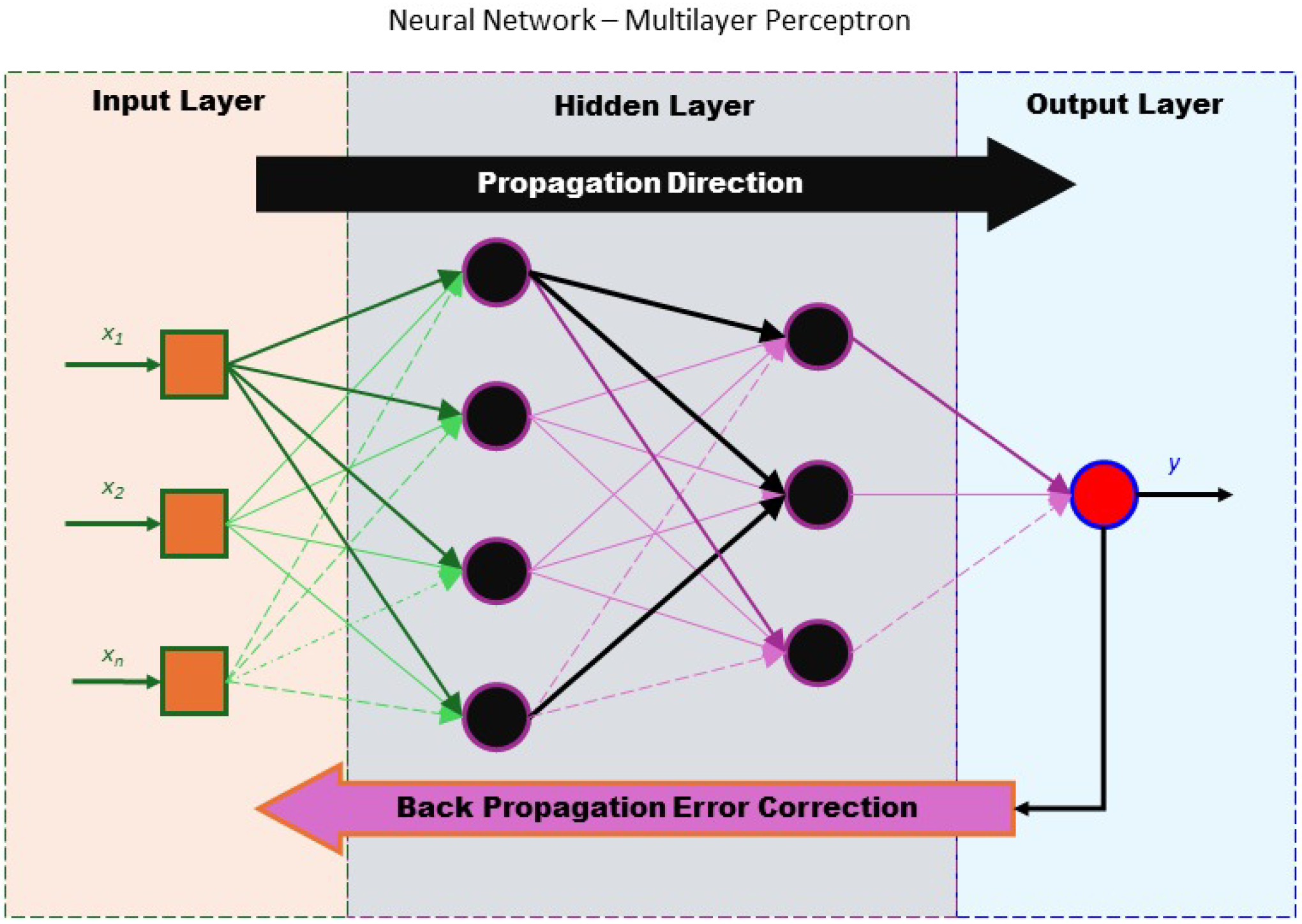
The central idea of artificial neural networks (ANN) was developed based on models of biological neurons, where the interconnection between several neurons forms a neural structure. Its typology has made it a powerful tool in solving different types of systems due to its high generalization ability. Its most general configuration consists of the use of input layers, multiple hidden layers and output layers, and for each variable applied to the input, a weight is assigned, which is multiplied by each input and are combined linearly, as shown in Figure 2.
These values are used as input to the hidden layers, where new weights are assigned to each input and new linear combinations of the values are performed in the hidden layers so that there is only one output in each neuron [12,29]. The value available at the output can be defined by
y j = Φ i = 1 m ω i j x i + ω i 0 ,
where x i represents the input neuron, ω i j the weight assigned between the i-input layer neuron and the j-hidden layer neuron, and Φ is the activation function.
With the evolution of computing power, different types of neural networks were developed, evolving to adapt to each specific type of problem. One of the variations that brought great results and became great bases are deep learning techniques, which include Recurrent Neural Networks (Gated Recurrent Unit GRU) and Long-Short-Term Memory (LSTM), which emerged as a solution so that information applied in the most initial layers of the neural network was not lost. The LSTM was implemented with a function that allows weights to be applied to the network input information in the hidden layers, and according to the weight assigned, this information is inserted into a memory cell. Information that has a higher weight has greater relevance, thus allowing the network to select which data is most important and should remain stored in order to achieve better network training [30]. Therefore, for LSTM, the values at a later stage can be defined by
C t = C t 1 ( f u ) t + ( i u ) t ( tanh ( W c x t + W H C H t 1 + b c ) ) ,
where W represents the weights of each stage, b is the bias variable, H t 1 represents each unit of the hidden layer, C t represents the current stage of the data, C t 1 represents the previous stage of the data, x t is the variable analyzed itself and ( f u ) t and ( i u ) t are defined according to the methodology described by Shahid [30].
In the application developed in this work, 50 neuron units were used in each layer of the neural network. The activation function used was the hyperbolic tangent (tanh). Sixty epochs were defined, which represents the number of times the model analyzes the training set to indicate its output value. Furthermore, the 30 days of previous input data would be used to predict each output value.

2.3.2. Sarimax

Time series data have a great variability in patterns, but for a model to be able to make predictions reliably, it is necessary to prove that the series is stationary. To this end, there are some techniques capable of removing the impacts of the periodicity of the data studied by adjusting the values to the samples of the complete set, such as seasonal autoregressive integrated moving average (SARIMA). Despite being a powerful technique, it does not have the ability to include influences external to the analyzed time series, for this purpose the SARIMAX technique was developed [30].
The SARIMA technique expresses the characteristics of time series through the parameters p, d, q, s, where p expresses the number of seasonal autoregression terms, q expresses the number of moving average terms, d represents the number of seasonal differencing required to make the series stationary and s expresses the number of observations in a season. The SARIMAX method uses the same parameters as SARIMA but incorporates the parameter r to express the information of the variable external to the time series [31]. The following equation expresses the SARIMAX technique,
Sarimax ( p , d , q , s , r ) = Sarima ( p , d , q , s ) + t = 1 r γ r x .
The parameter s is responsible for representing the period of analysis of the time series; as there is a seasonal pattern in the analyzed data, the value 12 was defined for the parameter s, which represents the 12 months of the year. In addition, a past observation was defined to predict the current value of the model, both for the auto-regression parameter and for the moving average and differentiation parameters.

2.3.3. Support Vector Regressor (SVR)

The SVR technique is the result of an extensive evolution of pattern recognition algorithms. Around the 1930s, a first algorithm of this nature was suggested, which was composed of an n-dimensional matrix containing covariance vectors between two normal population distributions. Around the 1960s, the first algorithms that considered networks between the evaluated values emerged. The first considered perceptron networks consisted of connected neurons, where each neuron implemented a separation hyperplane, forming a separation surface for parts of the data [32].
A few years later, a technique for mapping input vectors from a feature space was implemented, where special properties for decision-making were initially inserted so that linear decisions could be made to characterize the data. This technique was called support-vector network and it consists of creating optimal hyperplanes that are those that have as a result of a linear decision function the maximum margin between vectors of two different classes [32,33].
According to the technique, an optimal hyperplane can be found by w 0 · z + b 0 = 0 , where w 0 represents the weights of each position vector within the feature space, b 0 represents the bias and z are the vectors in the feature space, in which the support vectors can be found by the linear combination of the weights given by w 0 = s u p p o r t v e c t o r s α i z i . This technique can be used for problems where the objective is to separate data into different classes or to perform a regression of an output through the available inputs. When used for the first purpose, it is called SVC (Support Vector Classifier), when it has the second purpose, it is called SVR (Support Vector Regression).

2.3.4. Random Forest (RF)

The random forest technique is part of the class of methods called aggregation. Its main idea is closely linked to the idea behind decision tree algorithms, where a node is created for each evaluation so that a decision can be made. For example, to find out whether there will be people at the beach on a cloudy day, a decision node is created to check the days when there were people at the beach, and the classification as positive or negative will be made according to the established conditions. The result found in a higher node will lead to another node checking other conditions until the conclusion of the problem analyzed is reached. In the decision tree technique, the first node, which is also called the root node, must always be defined so that the next branches can be created from it. The definition of the root node is performed through an entropy algorithm or the Gini Index. In the random forest technique, the definition of this node does not happen in the same way. It uses resampling techniques of the available data so that it is possible to repeat some variables. With this, the algorithm will randomly choose two or more variables and then perform the necessary calculations with the selected samples, and thus define which one will be used in the first node. To assign the analyzed variable in the subsequent node, two or more variables will be chosen, excluding those previously chosen, and this sequence will be repeated until the end of the process in the construction of one of the trees [34].
However, as the name of the technique suggests, several decision trees are constructed to form a forest. If the problem studied requires regression, after the creation of the random forest, the final result presented will be the average of the values calculated by all the trees in the forest. This technique is powerful because it allows the comparison of numerous scenarios for the same set of variables, in addition to helping to avoid overfitting of the model. However, depending on the number of trees chosen, it may require greater computational cost [35].

2.4. Metrics

In order to evaluate the accuracy of the model, some metrics were calculated, including the Mean Absolute Error (MAE), Root Mean Squared Error (RMSE), the Coefficient of Determination (R2), and the Willmott index d, whose equations are
MAE = 1 n i = 1 n p i p ^ i ,
RMSE = 1 n i = 1 n p i p ^ i 2 ,
R 2 = 1 i = 1 n ( p i p ^ i ) 2 i = 1 n ( p i p ¯ ) 2 ,
d = 1 i = 1 n ( p p ^ ) 2 i = 1 n ( p p ¯ ) 2 ,
where the parameter p expresses the original value of the variable, p ^ expresses the estimated value, and p expresses the average of the original value of the variable. P i are the values predicted by the model or simulated, O i are the measured or observed values and O ¯ are the averages of the observed values. The Willmott index, which is very effective in evaluating the accuracy of the applied model, varies between 0 and 1. It was used to verify all the techniques used in this work in addition to each metric mentioned previously.

3. Results and Discussion

3.1. Variations in Meteorological Parameters

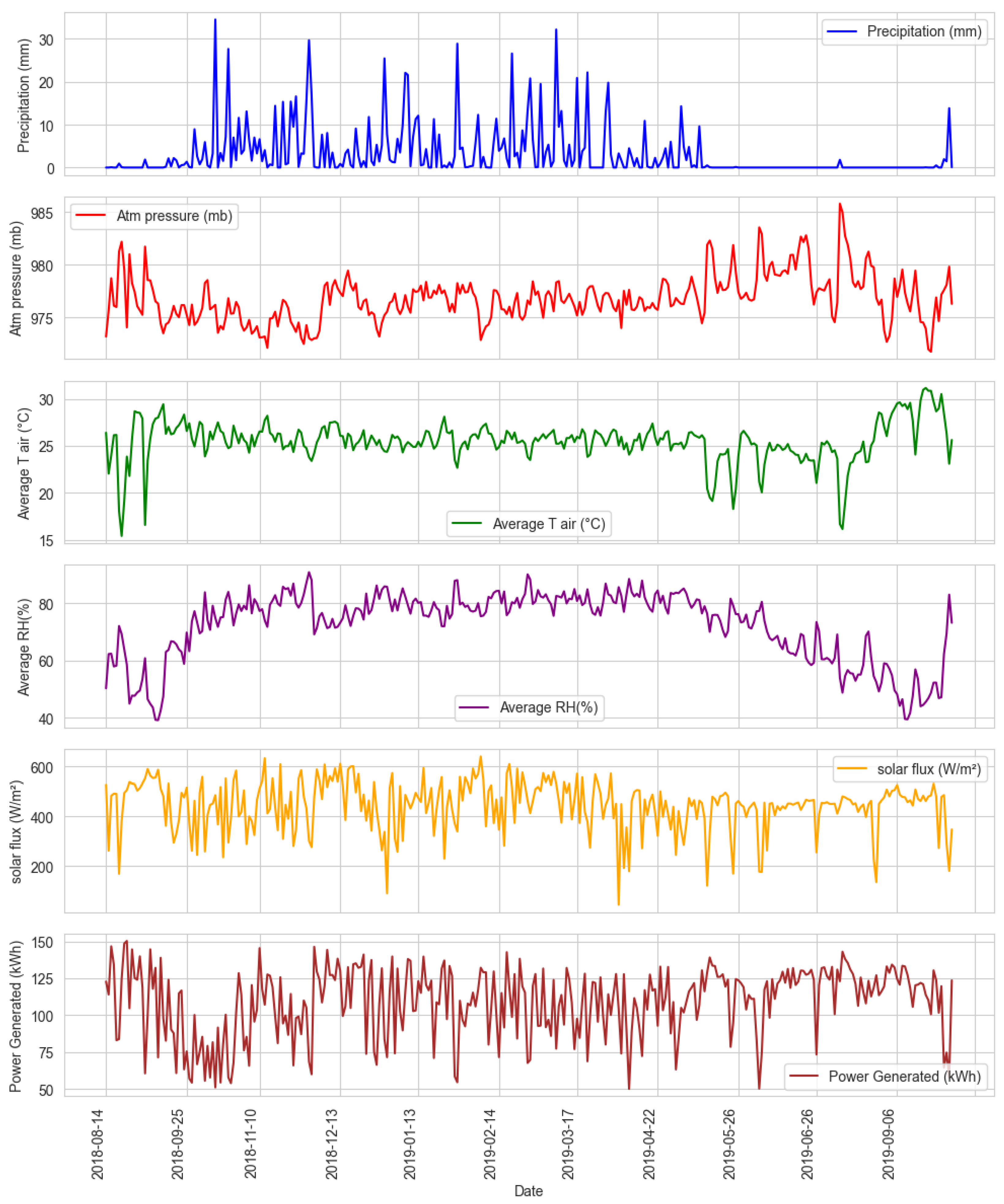
The data collected from the meteorological stations allows a complete characterization of the region’s climate. Through them, it is possible to verify that the months of June to October are the dry season in the region, and between the months of November and May is the rainy season, which is demonstrated by both the precipitation index and the relative humidity, which is shown in Figure 3. It also shows that there are periods of the year, within the dry season, in which the relative humidity reaches the level of 40%.
In addition to relative humidity reaching very low values during the dry season, the highest temperatures of the year are also experienced during this season. Figure 3 also shows that there are some days with low or mild temperatures during this season, which may be associated with the entry of cold air masses from other regions of the country. However, as this was not the objective of this study, this analysis was not performed. Another aspect that draws attention is the amplitude of the temperature variation measured during this season, for example between 4 and 5 September 2018, where a large variation in the average temperature was observed, increasing from 16 °C to 27 °C. Analyzing the complete series of data, it was observed that the period of lowest temperatures and largest thermal amplitudes was repeated throughout the years, thus demonstrating an annual pattern.
Analyzing the annual pattern for the energy generated by the photovoltaic plant, it was noted that the variability in its values is strongly related to the variables studied. In Figure 3, it is possible to compare the values of energy generated with the variations in temperature. It is possible to see that at the beginning of September, precisely when the temperature drops sharply, there is also a very sharp drop in the value of the energy generated. As previously mentioned, in this same period, the lowest values of relative humidity and low precipitation values were also found. Another interesting observation is the moments of low solar flux values that are also accompanied by a drop in energy generation values. Immediately after the moment in which solar flux increases again, the energy generated also follows suit, increasing its value.
Combining the information on the low temperatures of the period, the low precipitation rate and the low percentages of relative humidity, it is possible to make an empirical statement that during this period there was an entry of cold air masses into the region. If it is possible to consider this hypothesis, it is possible to understand the reason for the reduction in energy generated by the photovoltaic plant, which can corroborate the results found by Jadhav [36], which shows that clouds located at lower levels of the atmosphere can impact the reduction in solar radiation by approximately 44%.
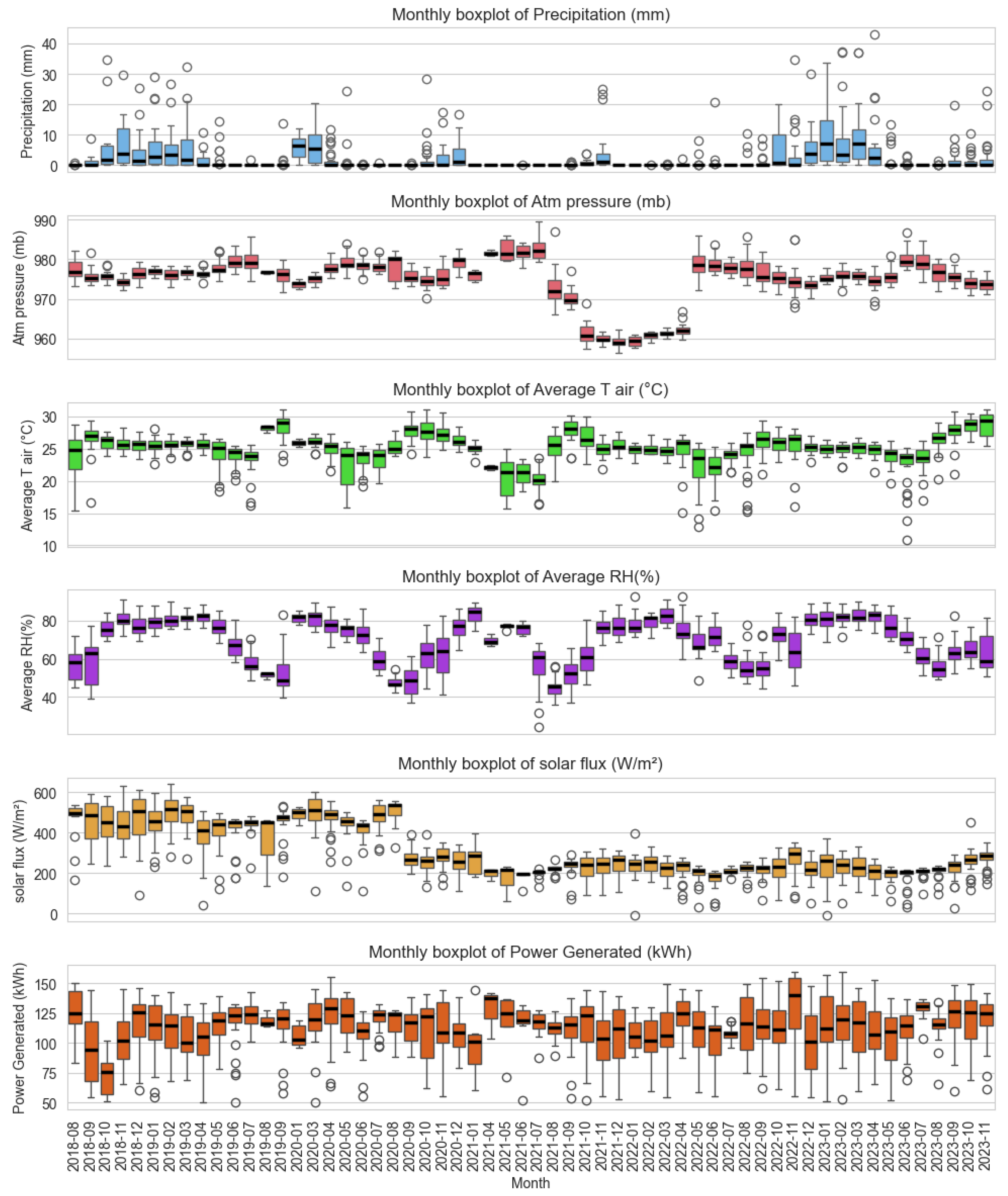
Therefore, it is possible to verify that the consideration of meteorological variables in the modeling of energy generated by photovoltaic plants is of vital importance to achieve better results in their implementations. A better understanding of the variables is demonstrated in Figure 4, through the boxplots of all the variables analyzed. It is seen that some variables have fewer values outside the confidence interval than others, such as relative humidity and temperature. The energy generated shows a greater number of outliers; however, the vast majority of them are below the confidence interval. This is due to the high possibility of generation data being lost, due to a lack of internet connection or maintenance carried out on the photovoltaic plant.
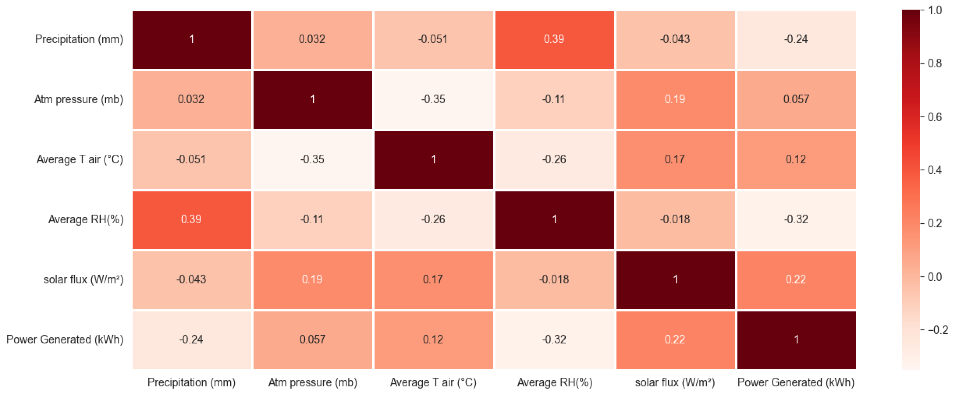
To verify how input variables relate to energy generation, a heat map was created, which shows the strength of the correlation between each of the observed variables.
Although it is possible to make some inferences when analyzing the variables studied, the heat map in Figure 5 shows that the correlations between one isolated variable and another are very weak, which makes it difficult to achieve robust modeling when performing analyses in isolation. For this reason, the machine learning techniques applied in this study are of great value, since through them it is possible to analyze the output variable (energy generated) in relation to all other input variables.

3.2. Evaluating the Performance of Machine Learning Models

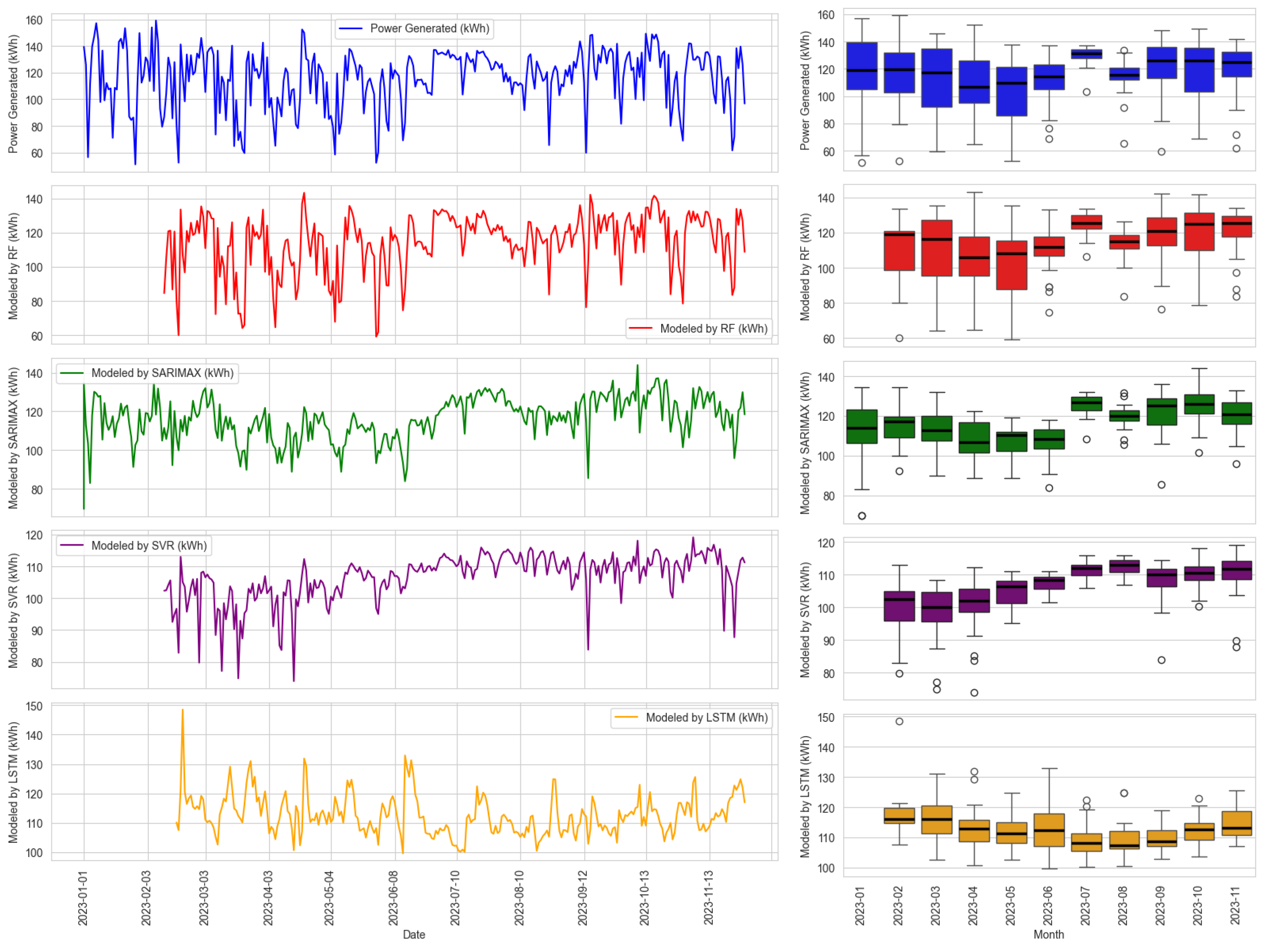
The application of machine learning techniques returned very varied results with characteristics that reflect each methodology used. Figure 6 allows the analysis of the results presented by the models, where the real values of the energy generated by the photovoltaic plant and the value returned by the application of each technique are shown so that comparison is possible. In Figure 6, it is possible to verify a very strong relationship between the Random Forest (RF) technique and the real values, since the graph of the RF values is very similar to the graph of the real values. It is possible to see that at times when there are negative peaks in the real values, the RF graph also shows a negative peak, however, overestimating the values in this case.
Another point that can be observed in Figure 6 is a reasonable result of the SARIMAX technique, as it is able to capture the negative peaks and also the moments when the real values start to increase, as is the case with the RF technique. This result of the SARIMAX technique is interesting, because unlike the other three techniques, it considers for analysis the time series of the real energy generated and the influence of a variable external to the series in question. To define the external variable, the information presented in the heat map in Figure 5 was used, which shows a negative correlation between the relative humidity and the energy generated, which indicates a decrease in one in relation to the other. Although there is a relative capture of reality, it is possible to see that there is a large error between the graph of the SARIMAX technique and the real values.
Figure 6 shows that the SVR and LSTM techniques deviate greatly from the real values, presenting a strong underestimation of the generated energy values at times when the real values are higher and an overestimation at times when the real values present negative peaks. Another aspect visualized is that the results for these two techniques tend to have low variability, which is easy to see through the boxplot of the models available in Figure 6, which shows the median of these two techniques varying very little.
The boxplots in Figure 6 also point to the strong correlation between the values found by the RF technique and the real values. In Figure 6, it is easy to see that the maximum and minimum values of the RF technique are very similar to the real values, as the technique presents minimum and maximum values of 58 kWh and 143 kWh, respectively, while the real values have minimum and maximum values of 53 kWh and 159 kWh, respectively, in January 2023. In addition, the number of outliers indicated by the RF technique also has great similarity with the number of outliers in real data, and of the 12 months in Figure 6, this number is only different in 4.
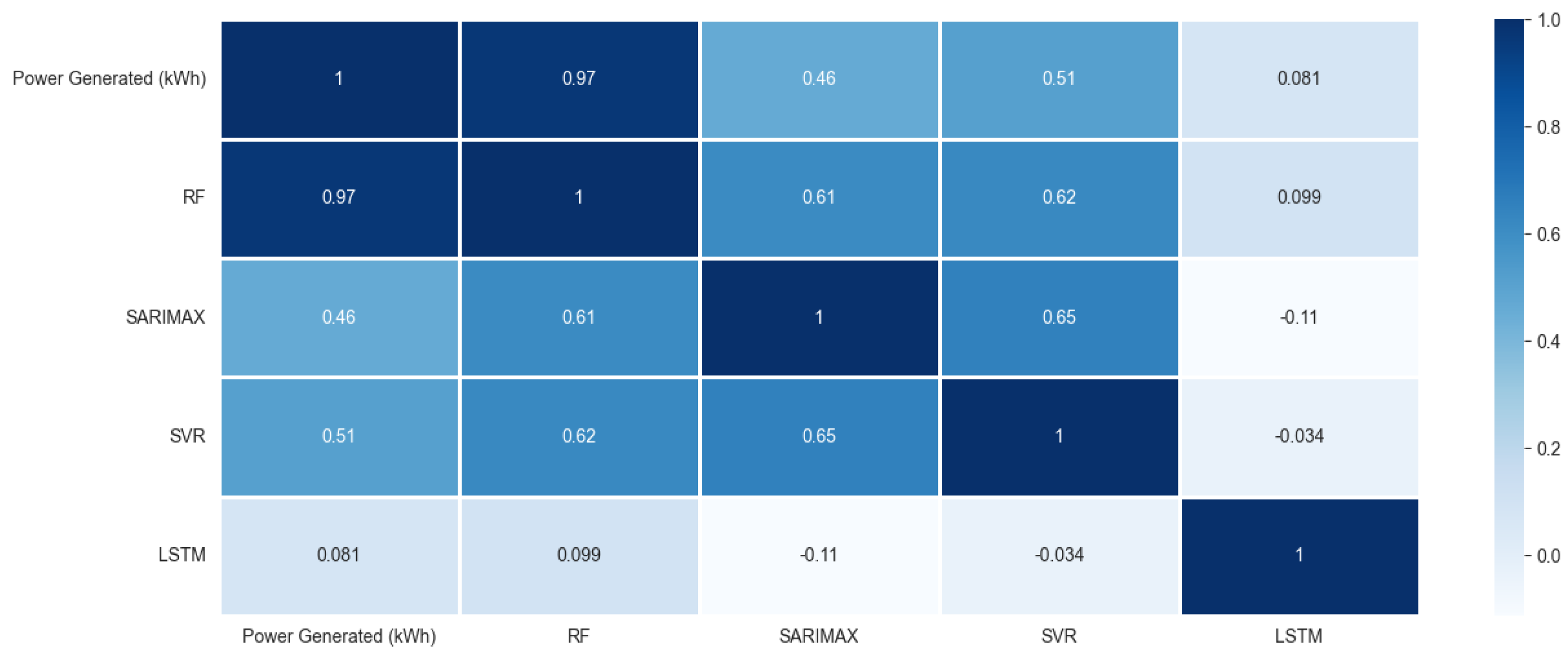
The correlations between the values of the model presented by the four techniques were calculated, so that more realistic information could be extracted about which technique would best reflect reality. The calculated correlations were presented through the heat map available in Figure 7, and with this map it is more evident which model best relates to the real values of energy generated.
In addition to the correlations in Figure 7, all the metrics described in Section 2.4 were calculated to compare the models. These metrics can be seen in Table 2. When analyzed, it is possible to see what the graphs in Figure 6 showed. Table 2 clearly shows the difference between the errors of each model, with the LSTM technique presenting the highest MAE and lowest R2, approximately 17.49 and 0.0258, respectively.
The RF technique presents the lowest absolute error, being the most accurate of all the techniques applied. An important point of the result presented is the Willmott Index, and the value found of 0.9716 is very satisfactory because it is much closer to the ideal than the value found with all the other techniques, since this index varies between 0 and 1, the R2 of the RF technique is also the highest found, reaching the value of 0.9016. This result can be directly linked to the nature of the technique, because while the SVR analyzes the problem as a whole and makes inferences about it, the random forest technique implemented 600 different scenarios for the same problem, since the creation of 600 trees was defined at the beginning of its application.
Regarding the SARIMAX technique, as mentioned previously, it presents smaller errors than the SVR and LSTM techniques, despite it considering a smaller number of variables than the other techniques.
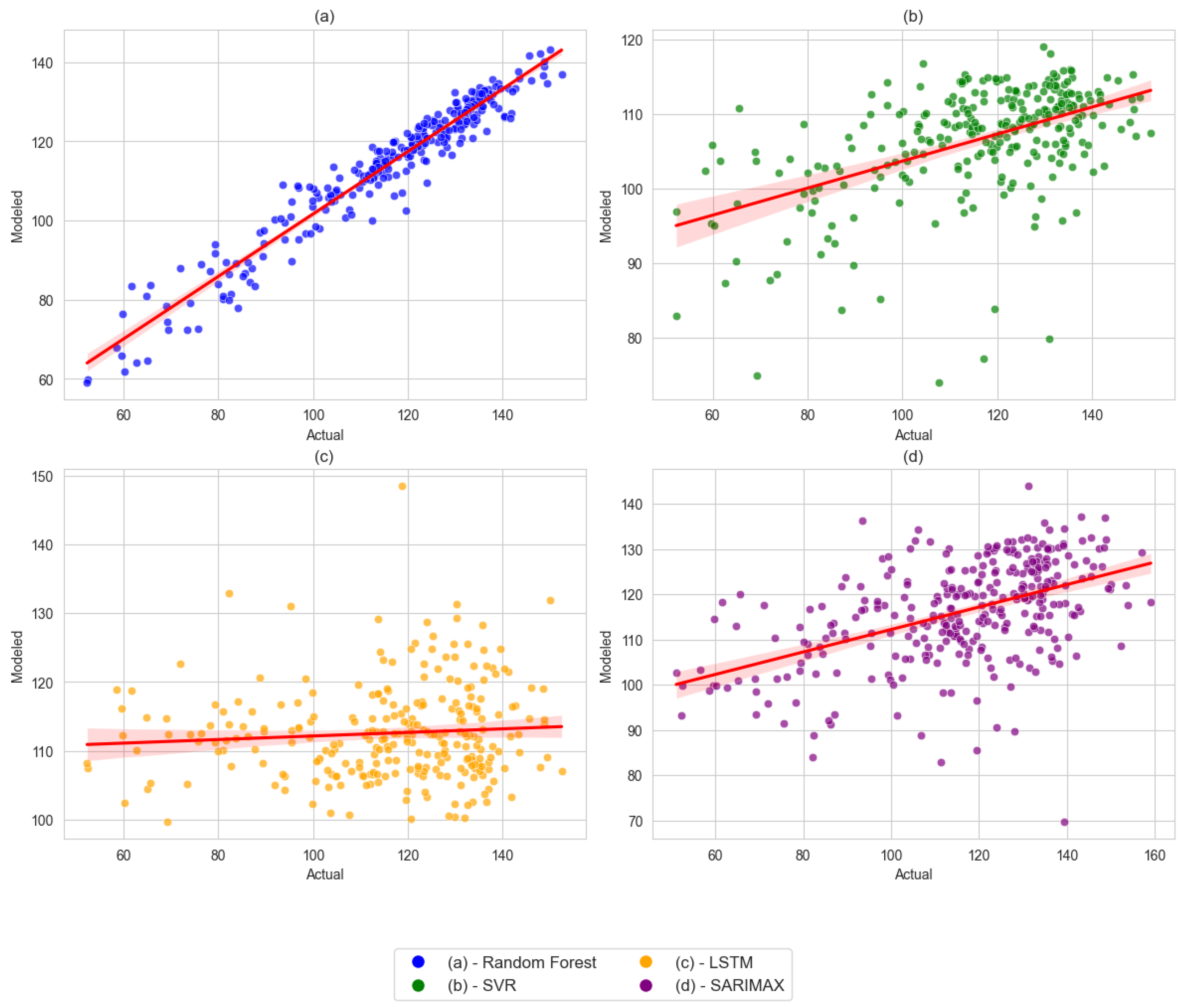
Analyzing the values shown in Table 2, it is possible to verify that the predictions of the LSTM and SVR techniques are unable to reflect the reality of the energy generation values. This is because, in addition to there being very large errors, the model patterns given by R2 and the Willmott index show that there will be a very large dispersion between the values estimated by the LSTM technique and the real values. This reality can be visualized in Figure 8, which shows the dispersion of the values presented by the four models, namely random forest (Figure 8a), SVR (Figure 8b), LSTM (Figure 8c), SARIMAX (Figure 8d).
In addition to evaluating the metrics presented in Table 2, a computational cost analysis was performed for each modeling technique. Each model’s script was executed following a specific procedure: first, each script was run once, and upon completion, it was executed three additional times consecutively. The total execution time from the initial run was recorded. From the three consecutive runs, the average execution time, the memory usage at the time of measurement, and the peak memory consumption throughout the entire process were calculated. The results of this computational cost evaluation are summarized in Table 3.
Through computational cost analysis, it is possible to draw different conclusions than those obtained from the values in Table 2. This is because Table 3 indicates that the SVR technique has the shortest processing time, which may represent a positive result depending on the application. On the other hand, regarding memory consumption, the SVR technique consumes the most memory during routine execution. Unlike SVR, the LSTM technique had the longest processing time, which may be related to the complexity of its architecture. However, among the four techniques, LSTM had the second lowest memory consumption in consecutive executions.
The LSTM neural network type was created to enable the storage of information about input variables for a longer period, so that it could be accessed, if necessary, in future iterations within the implementation of a neural network. Each layer will store information about the temporal dependencies learned from the data; for the available data, the use of 60 epochs was defined for the LSTM used. An edit of the LSTM parameters was also performed, with the aim of improving the model’s estimation using a Scikit Learn library called Gridsearch.
For its application, some parameters that the programmer considers important for improving the estimates must be defined, and several different values or configurations can be defined for each parameter. The library inserts the different values chosen for each defined parameter and runs the intended model to compare the results found with its use, and at the end selects which values or configurations of the parameters return the best results. The library’s return was that the best parameters and their values were batch size: 16; epochs: 30; model activation: sigmoid; model optimizer: adam; model units: 128. These parameters were assigned to the LSTM, which was applied again to the data. However, there was no improvement in the estimation given by the technique even with the application of this method, obtaining as a final result the dispersion shown in Figure 8.
Figure 8b also shows the results indicated by the errors in Table 2 for the model given by the SVR, since it shows the large dispersion of the modeled values in relation to the regression line. In Figure 8b, it is possible to see that the SVR model is able to capture the trend of the values and the slope of the angular coefficient of the trend line of the real values. However, there is a large dispersion of the trend line of the modeled values, even greater than that presented by the LSTM technique visualized in Figure 8c, which does not reflect good results presented by the model. As previously mentioned, the SARIMAX technique shows an interesting result, given its characteristics described in Section 2.3. The slope of the trend line of the SARIMAX technique in Figure 8d shows that the technique is able to insert the values in a region with a good relationship with the real data, and for this type of graph, the closer the trend line is to 45°, the greater the power of the technique in returning values close to the real.
Despite this, the results of this technique show a large dispersion of the trend line in Figure 8d, which had already been pointed out in Table 2 by the model metrics. Another interesting result is that the results of the RF technique also show little dispersion in relation to the trend line seen in Figure 8a, which denotes a significant difference from the results presented by the other techniques. In addition to the fact that the estimated values show a small dispersion in relation to the trend line, the slope of the line is very close to 45 , which would be a point at which the model would completely reflect the real values.
Therefore, the comparison between the four models studied shows that depending on the need of the study, the availability of data and the desired precision, there is a model that may present a better cost-benefit in its implementation. For example, if all the variables considered in the present study are available, there is sufficiently large computational power and a need for high precision of the modeled values, it is ideal to use the model given by the random forest technique.
However, if high precision of the returned values is not required, there are two methods that can be used: SVR and SARIMAX. The factor that will help you choose which of the two to use is data availability. If all variables are available, you can use the SVR method and obtain a good result in predicting the values with reasonable accuracy. However, the SARIMAX method is the most suitable if you have relative humidity data in the desired region, as it can deliver a result very close to the real one, even if it uses only one variable as input.
In addition to data availability, computational cost is an important parameter for method selection. According to the information shown in Table 3, although the random forest method requires more input variables, it has the lowest computational cost among the four techniques used, demonstrating its robustness at a very low cost. However, its execution time is long compared to the other three methods, ranking third in terms of execution time.
The results found by the modeled values show a strong relationship between meteorological variables and energy generation. Although no solar radiation extinction variable, no cloud cover analysis, and no optical evaluation of solar radiation were used in the analysis, the random forest technique was able to return values of energy generated with satisfactory accuracy, a result that is greatly influenced by the nature of the joint analysis algorithms [12].
The study also demonstrates that the application of robust techniques such as random forest in photovoltaic energy generation analyses can help meet the SDGs, especially SDG 7, which has as its theme “Ensure access to affordable, reliable, sustainable and modern energy for all” [37], as the use of more assertive tools in generation forecasts can provide greater security in the expected return of the system, avoiding oversizing and unnecessary expenses, which leads to an increasingly sustainable use of photovoltaic technology.

4. Conclusions

In this study, four different machine learning techniques were applied to model the energy generated by a photovoltaic plant through the relationship with meteorological variables. Of the techniques applied, three of them allowed the analysis of multiple input variables to model the dependent variable (SVR, LSTM and RF) and only one allowed the analysis of an endogenous variable as a function of an exogenous variable (SARIMAX). Among them, the one that presented the highest accuracy was random forest, with R2 and Willmott index of 0.907 and 0.9716, respectively.
This result is very interesting because the study did not use radiation flux or any variable for solar radiation extinction as input variables. Even so, it was possible to find a model for predicting the energy generated with high accuracy. This reinforces the importance of considering meteorological variables when sizing photovoltaic plants, making the planning of their implementation more effective and the energy generation process more efficient.
One aspect that was not analyzed in the study was the impact of clouds and particulate matter on energy generation. Although the variables studied have a certain relationship with the incidence of clouds, no technique capable of directly quantifying the effect of aerosols and clouds was used. Another approach that could be implemented in future studies is modeling with higher forecast frequencies, such as hourly, which was not possible in this study due to the unavailability of power generation data with such frequencies.
Despite the excellent performance found using the RF technique, the study found a very low correlation between the input variables, which creates a gap that could be addressed in future studies. The exploration of how the RF technique extracts information from weakly correlated data can be analyzed using techniques such as feature importance analysis.
Therefore, the use of the RF technique, which performed best in this study, can assist decision-makers in defining optimal scenarios for implementing this type of power generation plant, as it can be applied to different locations so that the results can be compared, leading to the definition of locations with favorable meteorological conditions for generation.

Author Contributions

Conceptualization, D.d.O.M.; methodology, D.d.O.M. and J.G.d.S.; software, B.N.d.C.; validation, B.N.d.C. and D.d.O.M.; formal analysis, J.G.d.S.; investigation, R.d.S.P.; data curation, B.N.d.C. and R.d.S.P.; writing—original draft preparation, B.N.d.C., D.d.O.M., M.S.B., N.N.d.O. and J.G.d.S.; writing—review and editing, B.N.d.C., D.d.O.M. and J.G.d.S.; visualization, D.d.O.M.; supervision, R.d.S.P. and D.d.O.M. All authors have read and agreed to the published version of the manuscript.

Funding

Conselho Nacional de Desenvolvimento Científico e Tecnológico (CNPq), code 174708/2023-8 and Programa de Grande Escala Biosfera-Atmosfera na Amazônia (LBA) n° 037/2023.

Institutional Review Board Statement

Not applicable.

Informed Consent Statement

Not applicable.

Data Availability Statement

Data will be provided upon request.

Acknowledgments

This research was partially funded by Conselho Nacional de Desenvolvimento Científico e Tecnológico (CNPq), code 174708/2023-8 and Programa de Grande Escala Biosfera-Atmosfera na Amazônia (LBA) n° 037/2023.

Conflicts of Interest

The authors declare no conflicts of interest. The funders had no role in the design of the study; in the collection, analyses, or interpretation of data; in the writing of the manuscript; or in the decision to publish the results.

References

  1. Gernaat, D.; de Boer, H.D.; Daioglou, V.; Yalew, S.; Müller, C.; van Vuuren, D.V. Climate change impacts on renewable energy supply. Nat. Clim. Change 2021, 11, 119–125. [Google Scholar] [CrossRef]
  2. Solaun, K.; Cerdá, E. Climate change impacts on renewable energy generation. A review of quantitative projections. Renew. Sustain. Energy Rev. 2019, 116, 109415. [Google Scholar] [CrossRef]
  3. Osman, A.; Chen, L.; Yang, M.; Msigwa, G.; Farghali, M.; Fawzy, S.; Rooney, D.W.; Yap, P. Cost, environmental impact, and resilience of renewable energy under a changing climate: A review. Environ. Chem. Lett. 2022, 21, 741–764. [Google Scholar] [CrossRef]
  4. Khan, S.A.; Tao, Z.; Agyekum, E.B.; Fahad, S.; Tahir, M.; Salman, M. Sustainable rural electrification: Energy-economic feasibility analysis of autonomous hydrogen-based hybrid energy system. Int. J. Hydrogen Energy 2025, 141, 460–473. [Google Scholar] [CrossRef]
  5. Yalew, S.; van Vliet, M.V.; Gernaat, D.; Ludwig, F.; Miara, A.; Park, C.; Byers, E.; Cian, E.D.; Piontek, F.; Iyer, G.; et al. Impacts of climate change on energy systems in global and regional scenarios. Nat. Energy 2020, 5, 794–802. [Google Scholar] [CrossRef]
  6. Cronin, J.; Anandarajah, G.; Dessens, O. Climate change impacts on the energy system: A review of trends and gaps. Clim. Change 2018, 151, 79–93. [Google Scholar] [CrossRef]
  7. Song, Z.; Liu, J.; Yang, H. Air pollution and soiling implications for solar photovoltaic power generation: A comprehensive review. Appl. Energy 2021, 298, 117247. [Google Scholar] [CrossRef]
  8. Dhake, H.; Kosmopoulos, P.; Mantakas, A.; Kashyap, Y.; El-Askary, H.; Elbadawy, O. Climatological Trends and Effects of Aerosols and Clouds on Large Solar Parks: Application Examples in Benban (Egypt) and Al Dhafrah (UAE). Remote Sens. 2024, 16, 4379. [Google Scholar] [CrossRef]
  9. REN21. Renewables 2020 Global Status Report: Chapter 01—Renewable Energy in 2019. In Renewable Energy Policy Network for the 21st Century; REN21: Paris, France, 2020. [Google Scholar]
  10. Dutta, R.; Chanda, K.; Maity, R. Future of solar energy potential in a changing climate across the world: A CMIP6 multi-model ensemble analysis. Renew. Energy 2022, 188, 819–829. [Google Scholar] [CrossRef]
  11. Brazil Breaks Record for Solar Energy Expansion in 2023. 2023. Available online: https://canalsolar.com.br/en/Brazil-records-record-expansion-of-solar-energy-in-2023/ (accessed on 13 May 2025).
  12. Chen, Y.; Yue, X.; Tian, C.; Letu, H.; Wang, L.; Zhou, H.; Zhao, Y.; Fu, W.; Xu, Z.; Peng, D.; et al. Assessment of solar energy potential in China using an ensemble of photovoltaic power models. Sci. Total Environ. 2023, 877, 162979. [Google Scholar] [CrossRef]
  13. Ali, M.G.; Hassan, H.; Ookawara, S.; Nada, S.A. Investigation of the performance enhancement of building-integrated photovoltaic system using evaporative porous clay applied in different building’s directions. J. Build. Eng. 2024, 82, 108292. [Google Scholar] [CrossRef]
  14. Ghazali Ali, M.; Hassan, H.; Ookawara, S.; Nada, S.A. Assessment of evaporative porous clay cooler for Building-Integrated photovoltaic systems via energy, exergy, economic and environmental approaches. Therm. Sci. Eng. Prog. 2024, 51, 102641. [Google Scholar] [CrossRef]
  15. Paletta, Q.; Terrén-Serrano, G.; Nie, Y.; Li, B.; Bieker, J.; Zhang, W.; Dubus, L.; Dev, S.; Feng, C. Advances in solar forecasting: Computer vision with deep learning. Adv. Appl. Energy 2023, 11, 100150. [Google Scholar] [CrossRef]
  16. Tang, Y.; Yang, K.; Zhang, S.; Zhang, Z. Photovoltaic power forecasting: A dual-attention gated recurrent unit framework incorporating weather clustering and transfer learning strategy. Eng. Appl. Artif. Intell. 2024, 130, 107691. [Google Scholar] [CrossRef]
  17. Chen, J.; Wen, Y.; Nanehkaran, Y.; Suzauddola, M.; Chen, W.; Zhang, D. Machine learning techniques for stock price prediction and graphic signal recognition. Eng. Appl. Artif. Intell. 2023, 121, 106038. [Google Scholar] [CrossRef]
  18. Gaviria, J.; Narváez, G.; Guillén, C.; Giraldo, L.F.; Bressan, M. Machine learning in photovoltaic systems: A review. Renew. Energy 2022, 196, 298–318. [Google Scholar] [CrossRef]
  19. Behera, M.; Majumder, I.; Nayak, N. Solar photovoltaic power forecasting using optimized modified extreme learning machine technique. Eng. Sci. Technol. Int. J. 2018, 21, 428–438. [Google Scholar] [CrossRef]
  20. Xu, J.; Wang, Z.; Li, X.; Li, Z.; Li, Z. Prediction of Daily Climate Using Long Short-Term Memory (LSTM) Model. Int. J. Innov. Sci. Res. Technol. (IJISRT) 2024, 9, 83–90. [Google Scholar] [CrossRef]
  21. Nwokolo, S.C.; Eyime, E.; Obiwulu, A.U.; Meyer, E.L.; Ahia, C.C.; Ogbulezie, J.; Proutsos, N. A multi-model approach based on CARIMA-SARIMA-GPM for assessing the impacts of climate change on concentrated photovoltaic (CPV) potential. Phys. Chem. Earth Parts A/B/C 2024, 134, 103560. [Google Scholar] [CrossRef]
  22. Zia, S. Climate Change Forecasting Using Machine Learning SARIMA Model. iRASD J. Comput. Sci. Inf. Technol. 2021, 2, 1–12. [Google Scholar] [CrossRef]
  23. Jiang, Y.; Zhang, T.; Gou, Y.; He, L.; Bai, H.; Hu, C. High-resolution temperature and salinity model analysis using support vector regression. J. Ambient. Intell. Humaniz. Comput. 2024, 15, 1517–1525. [Google Scholar] [CrossRef]
  24. Delbari, M.; Sharifazari, S.; Mohammadi, E. Modeling daily soil temperature over diverse climate conditions in Iran—A comparison of multiple linear regression and support vector regression techniques. Theor. Appl. Climatol. 2019, 135, 991–1001. [Google Scholar] [CrossRef]
  25. Silva, J.H.P.; Oliveira, M.D.F.; Santos, R.F.; Almeida, G.R. Performance of potato cultivars under different irrigation managements in a semi-arid climate. Rev. Ciências Agrárias Ambient. 2018, 25, 612–619. [Google Scholar] [CrossRef]
  26. Palácios, R.; Sallo, F.; Santos, A.; Nogueira, J.; Santana, F. Estimation of Direct Radiative Forcing of Aerosols on the Surface in the Pantanal-Cerrado Transition Region in the State of Mato Grosso, Brazil. Rev. Bras. Climatol. 2015, 16, 132–141. [Google Scholar] [CrossRef]
  27. Pérez-Ramírez, D.; Andrade-Flores, M.; Eck, T.F.; Stein, A.F.; O’Neill, N.T.; Lyamani, H.; Gassó, S.; Whiteman, D.N.; Veselovskii, I.; Velarde, F.; et al. Multi year aerosol characterization in the tropical Andes and in adjacent Amazonia using AERONET measurements. Atmos. Environ. 2017, 166, 412–432. [Google Scholar] [CrossRef]
  28. ISO 9060:2018; Specification and Classification of Instruments for Measuring Hemispherical Solar and Direct Solar Radiation. ISO Copyright Office: Geneva, Switzerland, 2018. Available online: https://www.iso.org (accessed on 13 May 2025).
  29. Vijh, M.; Chandola, D.; Tikkiwal, V.; Kumar, A. Stock Closing Price Prediction using Machine Learning Techniques. Procedia Comput. Sci. 2020, 167, 599–606. [Google Scholar] [CrossRef]
  30. Shahid, F.; Zameer, A.; Muneeb, M. A novel genetic LSTM model for wind power forecast. Energy 2021, 223, 120069. [Google Scholar] [CrossRef]
  31. Elshewey, A.M.; Shams, M.Y.; Elhady, A.M.; Shohieb, S.M.; Abdelhamid, A.A.; Ibrahim, A.; Tarek, Z. A Novel WD-SARIMAX Model for Temperature Forecasting Using Daily Delhi Climate Dataset. Sustainability 2023, 15, 757. [Google Scholar] [CrossRef]
  32. Cortes, C.; Vapnik, V. Support-vector networks. Mach. Learn. 1995, 20, 273–297. [Google Scholar] [CrossRef]
  33. Jändel, M. A neural support vector machine. Neural Netw. 2010, 23, 607–613. [Google Scholar] [CrossRef]
  34. Lahouar, A.; Ben Hadj Slama, J. Hour-ahead wind power forecast based on random forests. Renew. Energy 2017, 109, 529–541. [Google Scholar] [CrossRef]
  35. Kamińska, J.A. The use of random forests in modelling short-term air pollution effects based on traffic and meteorological conditions: A case study in Wrocław. J. Environ. Manag. 2018, 217, 164–174. [Google Scholar] [CrossRef] [PubMed]
  36. Jadhav, A.V.; Rahul, P.R.C.; Kumar, V.; Dumka, U.C.; Bhawar, R.L. Spatiotemporal Assessment of Surface Solar Dimming in India: Impacts of Multi-Level Clouds and Atmospheric Aerosols. Climate 2024, 12, 48. [Google Scholar] [CrossRef]
  37. Sustainable Development Goals. 2020. Available online: https://sdgs.un.org/goals. (accessed on 13 May 2025).
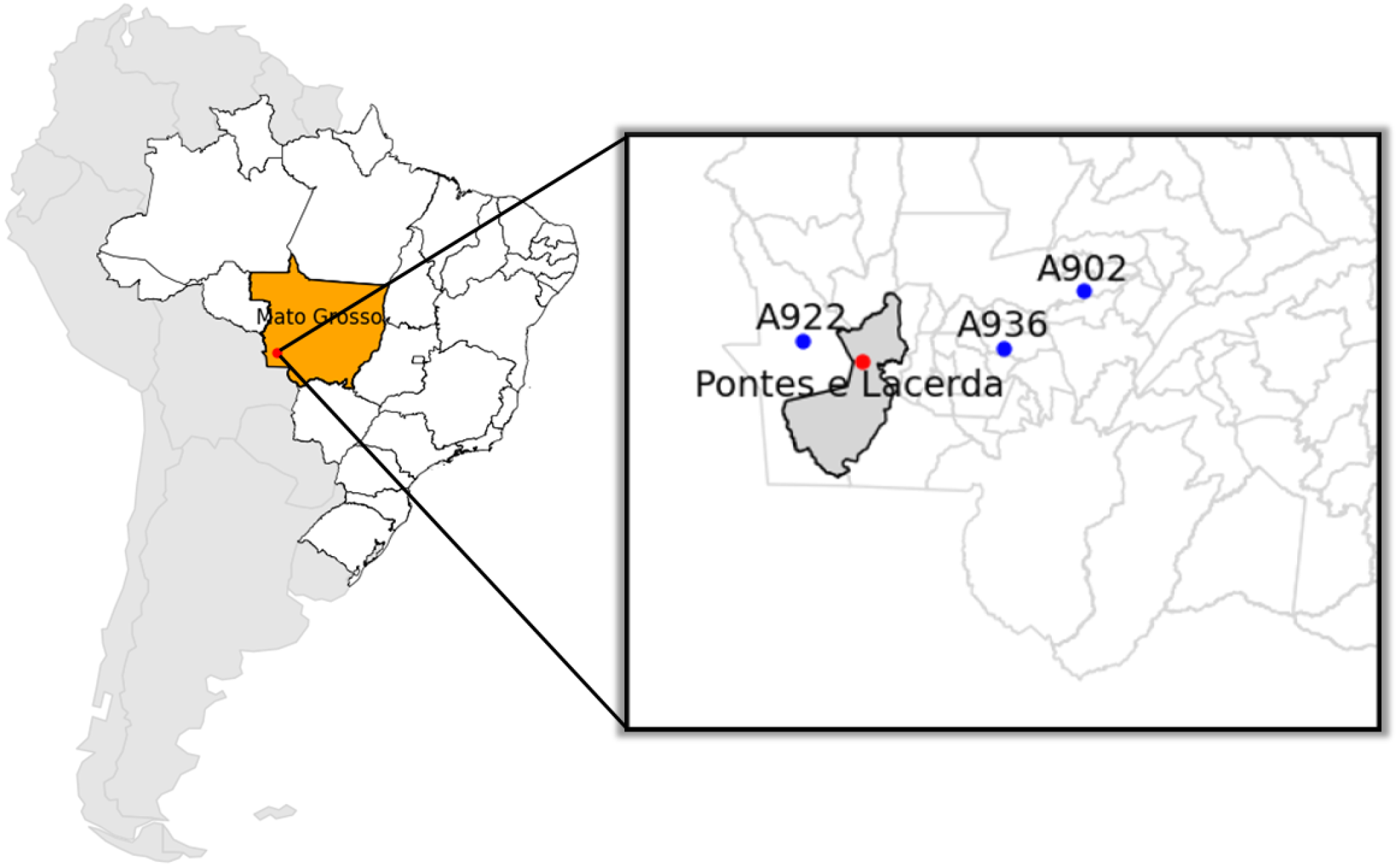
Figure 1. Location of study area.
Sustainability 17 07506 g001
Figure 2. Illustration of the layers of an artificial neural network.
Sustainability 17 07506 g002
Figure 3. Distribution of meteorological variables in the first 12 months of data.
Sustainability 17 07506 g003
Figure 4. Boxplots of the variables analyzed in the complete period.
Sustainability 17 07506 g004
Figure 5. Heat map with correlations between variables.
Sustainability 17 07506 g005
Figure 6. Real and modeled energy generated by the four techniques.
Sustainability 17 07506 g006
Figure 7. Heatmap of correlation between models.
Sustainability 17 07506 g007
Figure 8. Dispersion of the four prediction models.
Sustainability 17 07506 g008
Table 1. Station information including code, coordinates, altitude, data availability, and periodicity for selected locations in the state of Mato Grosso.
Station NameCodeLatitudeLongitudeAltitude (m)AvailabilityPeriodicity
Pontes e LacerdaA937−15.1344−59.3461272.531 January 2018–1 January 2024Daily
Salto do CéuA936−15.1247−58.1272300.831 January 2018–Present dayDaily
VBSTA922−15.0628−59.8731213.001 January 2018–Present dayDaily
Tangará da SerraA902−14.6500−57.4317440.011 January 2018–Present dayDaily
Table 2. Comparison between the metrics found for each model.
ModelMAERMSE R 2 d
LSTM17.632721.98310.07820.0028
SVR17.049920.67620.04360.5584
SARIMAX14.740719.25340.23770.6155
Random Forest4.91226.37780.90900.9720
Table 3. Comparison of the computational cost of each technique.
Model1st Run Time (s)Average Time (s)Current Memory (MB)Peak Memory (MB)
LSTM37.9335.518.0211.20
SVR0.100.0629.3931.24
SARIMAX3.873.421.40167.51
Random Forest7.273.720.020.86
Disclaimer/Publisher’s Note: The statements, opinions and data contained in all publications are solely those of the individual author(s) and contributor(s) and not of MDPI and/or the editor(s). MDPI and/or the editor(s) disclaim responsibility for any injury to people or property resulting from any ideas, methods, instructions or products referred to in the content.