Sustainable Data Construction and CLS-DW Stacking for Traffic Flow Prediction in High-Altitude Plateau Regions

Abstract

This study proposes a novel vehicle speed prediction model for plateau transportation—CLS-DW Stacking (Constrained Least Squares Dynamic Weighting Model Stacking)—which holds significant implications for the sustainable development of transportation systems in high-altitude regions. Research on sharp-curved roads on mountainous plateaus remains scarce. Compared with plain areas, data acquisition in such regions is constrained by government confidentiality policies, while complex environmental and topographical conditions lead to substantial variations in road alignment and elevation. To address these challenges, this study presents a sustainable data acquisition and construction method: unmanned aerial vehicle (UAV) video data are processed through road image segmentation, trajectory tracking, and three-dimensional modeling to generate multi-source heterogeneous datasets for both single-curve and continuous-curve scenarios. Building upon these datasets, the proposed framework integrates constrained least squares with multiple deep learning methods to achieve accurate traffic flow prediction. Bi-LSTM (Bidirectional Long Short-Term Memory), Informer, and GRU (Gated Recurrent Unit) are employed as base learners, and the loss function is redefined with non-negativity and normalization constraints on the weights. This ensures optimal weight coefficients for each base learner, with the final prediction obtained via weighted summation. The experimental results show that, compared with single deep learning models such as Informer, the proposed model reduces the mean squared error (MSE) by 1.9% on the single curve dataset and by 7.7% on the continuous curve dataset. Furthermore, by combining vehicle speed predictions across different altitude gradients with decision tree-based interpretable analysis, this research provides scientific support for developing altitude-specific and precision-oriented speed limit policies. The outcomes contribute to accident risk reduction, traffic congestion mitigation, and carbon emission reduction, thereby improving road resource utilization efficiency. This work not only fills the research gap in traffic prediction for sharp-curved plateau roads but also supports the construction of green transportation systems and the broader objectives of sustainable development in high-altitude regions.

1. Introduction

1.1. Research Background

Traffic flow prediction is a core component of intelligent transportation systems (ITSs) and encompasses three fundamental elements: traffic volume, density, and speed. Accurate traffic volume prediction can support traffic planning, traffic management and control, road safety assessment, and energy consumption estimation [1]. Density prediction contributes to traffic state evaluation and congestion mitigation, while speed prediction plays a critical role in preventing traffic accidents, optimizing traffic management, and enhancing safety. Therefore, vehicle speed is a core indicator for assessing traffic efficiency and safety [2].

Speed prediction, as an important branch of traffic flow prediction, is typically presented in the form of time series data. In urban traffic, the data also exhibits significant spatial features, which increases the complexity of model development. Thus, developing a model capable of accurately and efficiently predicting speed is not only a challenge to existing technologies but also holds substantial theoretical and engineering significance.

1.2. Related Work

Traditional prediction algorithms, such as the Autoregressive Integrated Moving Average (ARIMA) model [3], Markov Chain Prediction, Grey Prediction, and Kalman Filter, are based on statistical science, system science, and mathematical methods. However, these traditional algorithms have certain limitations in predicting traffic flow. Chandra et al. [4] argued that the ARIMA model cannot consider upstream and downstream information on the road and proposed a Vector Autoregression model for improvement. Shin et al. [5] considered that driver behavior is susceptible to environmental factors, introducing uncertainty and complexity, and used a Markov chain with speed constraints for speed prediction. Xiao et al. [6] noted that the first-order accumulation generating operator in the grey GM(1,1) (Grey Model(1,1)) model cannot effectively address seasonal factors, proposing a seasonal grey rolling prediction model based on the CTAGO operator for short-term traffic flow prediction. Cai et al. [7] found that real-world traffic flow data often contains non-Gaussian noise, rendering traditional Kalman filters unsuitable, and proposed a Kalman filter derived from the maximum entropy criterion to address this issue. However, these methods face challenges in modeling the complex nonlinear dynamics of traffic flow, and machine learning can be combined to enhance flexibility.

With the rise of Artificial Intelligence (AI), machine learning algorithms such as Support Vector Machine (SVM) [8], Random Forest [9], Multiple Linear Regression [10], Logistic Regression [11], K-Nearest Neighbors (KNNs) [12], and XGBoost [13] have been widely applied in traffic flow prediction. However, traditional regression methods often overlook spatial heterogeneity [14], while machine learning models have limitations in fully exploiting historical data; moreover, their prediction accuracy can deteriorate significantly when subjected to external disturbances.

As AI continues to develop, deep learning, as a subfield of machine learning, has gained increasing attention. The powerful feature extraction capabilities and end-to-end automated learning provided by deep learning offer a new methodology for traffic flow prediction. Yan et al. [15] used Deep Neural Networks (DNNs) to predict short-term vehicle speed as a DNN is the core model of deep learning that automatically learns complex features from data through multiple nonlinear transformations. However, ordinary neural network models are limited in their ability to learn data dependencies, resulting in poor performance when processing sequence data such as traffic flow. Thus, Recurrent Neural Networks (RNNs) [16] were introduced to handle sequence data. But RNNs perform poorly in capturing long-range dependencies, as gradient vanishing or explosion occurs during chain differentiation. To alleviate this issue, Long Short-Term Memory (LSTM) networks were proposed, which introduce cell and hidden states in the neuron structure and gating mechanisms to mitigate gradient vanishing and explosion problems, showing excellent performance in vehicle speed prediction [17]. Gated Recurrent Units (GRUs), a variant of LSTM, simplify the LSTM structure and have also been applied in speed prediction [18]. Traditional LSTM models are unidirectional, utilizing only historical information, and are unable to capture the impact of future moments on the current state. Therefore, Bidirectional LSTM (Bi-LSTM) was proposed to significantly enhance the model’s ability to handle traffic flow time series data [19]. However, as the sequence length increases, RNN-based models struggle to capture long sequence features. The Transformer model, introduced in 2017, addresses this issue and has shown great results in speed prediction [20].

In urban areas, due to the road network structure, traffic flow data often possesses spatial features. Convolutional Neural Networks (CNNs) have been applied in traffic speed prediction to extract spatial features [21], but CNNs’ dependence on Euclidean spatial grid data makes it difficult to handle non-Euclidean graph data [22,23]. Graph Neural Networks (GNNs) are more suitable for simulating the underlying graph structure of traffic data [24], and variants of GNNs, such as Spatio-Temporal Graph Convolutional Networks (STGCNs) [25], Graph WaveNet [26], Spatio-Temporal Graph Neural Control Differential Equations (STG-NCDEs) [27], and Spatio-Temporal Similarity Fusion Graph Adversarial Convolutional Networks (STSF-GACNs) [28], have been used for traffic flow prediction.

To improve prediction accuracy, researchers have attempted to use hybrid models for traffic flow prediction. Wang et al. [29] combined the ARIMA model and LSTM (ARIMA-LSTM) for short-term vehicle speed prediction. Bae et al. [30] applied Principal Component Analysis (PCA) and Multivariate Singular Spectrum Analysis (MSSA) to address the complexity caused by network size and data volume in prediction processes. Liu et al. [31] proposed a method for predicting off-road vehicle speeds based on Backpropagation Neural Networks (BPNNs) and LSTM.

The aforementioned AI methods primarily involve improving or hybridizing models to predict traffic flow, essentially using a single model for prediction. However, Amiri et al. [11] employed Stacking, an ensemble learning technique, which combined Random Forest (RF), K-Nearest Neighbors (KNNs), and XGBoost as base learners and Logistic Regression (LR) as a meta-learner to predict traffic flow. Compared to single models, Stacking offers better generalization, reflecting the strengths of different models. However, Stacking requires training multiple base models and a meta-model, and the cross-validation process used to generate predictions further increases computational costs.

In summary, the limitations of existing methods can be outlined as detailed in

Table 1. Summary of related work.

Reference	Method	Summary of Method	Limitations
[3]	ARIMA	Classical method based on traditional statistical theory	Cannot model the complex nonlinearity of traffic flow
[4,5,6,7]	Vector autoregressive models, Markov chains with speed constraints, seasonal grey rolling prediction model based on CTAGO operator, and Kalman filter based on maximum entropy criterion	Improved traditional methods
[9,10,11,12,13]	SVM, Random Forest, Multiple Linear Regression, Logistic Regression, KNN, and XGBoost	Classical machine learning methods	Limited ability to deeply mine historical data; easily affected by external noise
[15,16,17,18,19,20,21,22,23,24,25,26,27,28]	DNN, RNN, LSTM, GRU, Bi-LSTM, Transformer, CNN, GNN, and variants	Deep learning methods	Compared with ensemble learning, they lack multi-perspective understanding and data analysis capabilities
[29,30,31]	ARIMA-LSTM, PCA-MSSA, and BPNN-LSTM	Hybrid models
[11]	Stacking	Ensemble learning	High computational cost, limited interpretability

.

1.3. Contributions of This Study

This study selects three models—Bi-LSTM, Informer, and GRU—that have shown excellent performance in traffic flow and other time series data modeling as base learners and constructs a unique methodology called CLS-DW Stacking. Unlike traditional stacking strategies, where the meta-learner learns from the output training set of base learners using machine learning, our method innovatively integrates the predictions of each base learner, reasonably allocates weights to minimize loss, and ultimately yields the optimal prediction results. Compared to traditional methods, which can lead to information loss and overlook predictions from certain base learners during the meta-learning process, our approach demonstrates significant advantages in generalization ability and enhances model interpretability to some extent.

Unlike traditional speed prediction methods, as discussed in the literature review, past studies often employed either a single deep learning model or a hybrid model (which is essentially still a single deep model) for speed prediction. However, these single models tend to have many limitations and struggle to meet the complex requirements of speed prediction. On one hand, single models are prone to overfitting. Due to their reliance on specific assumptions, predictions can deviate significantly when applied to data outside of the training set. They are limited in their ability to understand and analyze data from multiple perspectives, making it difficult to capture the complex patterns and multidimensional feature relationships within the data. On the other hand, the generalization ability of a single model is also limited. When faced with different traffic scenarios and data distributions, a single model, lacking diversity, struggles to adapt to new data variations, leading to unstable and inaccurate predictions. However, integrating multiple deep learning models can not only effectively overcome the limitations of single models but also significantly improve prediction performance. By leveraging the collaborative effect of multiple models, the predictions of each model complement each other, and by considering the strengths of each model, a more comprehensive and accurate understanding of the complex patterns of speed changes can be achieved.

In the research process, we conducted a thorough analysis of the types and characteristics of sharp-curved roads, categorizing them into single sharp curves and continuous sharp curves. To ensure the reliability and accuracy of the results, we used drone technology to collect data from both types of sharp-curved roads and created heterogeneous multi-source datasets for each type. Furthermore, we applied the CLS-DW Stacking model to train both datasets, aiming to accurately predict vehicle speeds and provide data support for relevant authorities in formulating speed-limiting policies. The contributions of this study are as follows:

• A low-cost dataset creation method suitable for areas with limited data availability is proposed. Drone-captured video data is used as the source, processed through image segmentation, trajectory extraction, 3D modeling, and other data handling methods, combined with the characteristics of the curves, to create multi-source heterogeneous datasets for single curves and continuous curves.
• The traditional approach involves using a single model for prediction. In this study, we propose a method that integrates three deep learning models, assigning optimal weights to the models using a dynamic weighting method based on constrained least squares. The final prediction results are obtained by combining the outputs of these models. The experimental results show that the proposed framework, which integrates multiple models, achieves better prediction performance compared to a single model.

2. Feature Selection

Accurate speed prediction is crucial for ensuring traffic safety and reducing traffic accidents. When constructing a speed prediction model, the selected features should encompass the entire traffic system, as the traffic system is a complex system deeply integrating people, vehicles, roads, and the environment [32]. To ensure that the chosen features can accurately reflect vehicle speed on sharp curved roads in plateau mountain areas, the features must cover the entire traffic system, meaning they should reflect people, vehicles, roads, and the environment. Therefore, the selection of feature variables is of paramount importance.

(1) In the traffic system, people are the core element, mainly encompassing drivers and pedestrians. However, given the sparse population in plateau mountain areas, pedestrians have a negligible impact on traffic flow and can be ignored in this study. For drivers, their psychological state and driving behavior directly influence vehicle speed. This study focuses on key feature variables that can accurately reflect the driver’s psychological state and behavior. In scenarios such as meeting other vehicles or following another vehicle, drivers tend to concentrate and adopt cautious driving strategies to ensure safety. Therefore, this study will use the presence of oncoming traffic or following another vehicle as objective indicators of the driver’s psychological state. Additionally, the specific driving patterns of vehicles on curves—such as driving near the inside or outside of the lane, along the lane centerline, or occupying the lane—are considered direct manifestations of the driver’s behavior.

Thus, the features selected include whether the driver is encountering oncoming traffic, following another vehicle, and the vehicle’s specific driving behavior, aiming to comprehensively and accurately capture the driver’s psychological state and driving behavior characteristics.

(2) Larger vehicles generally have a greater turning radius and slower speeds compared to smaller vehicles. This study includes vehicle type as a feature variable to more accurately characterize vehicle behavior on curved roads. Additionally, acceleration is a key indicator that reflects a vehicle’s operating state and rate of speed change. Therefore, acceleration is also considered an important feature variable.

Thus, vehicle type and acceleration are selected as feature variables to more comprehensively capture the dynamic behavioral characteristics of vehicles on sharp-curved roads.

(3) Road curvature is an important indicator for evaluating road safety [33]. Modern road curvature consists of straight lines, circular curves, and transition curves. The curvature of a straight line is 0, while the curvature of a circular curve is 1/R. At the point where a straight line and circular curve meet, the curvature is discontinuous, which does not align with the vehicle’s trajectory, increasing safety risks. Therefore, transition curves are introduced as a means of creating a smooth transition between straight and circular curves. While scholars have proposed various forms for transition curves, such as cubic parabolas or clothoids, the spiral curve is preferred in China due to its simplicity and ease of calculation. The basic formula for the spiral curve is shown in Equation (1).

$$\mathrm{rl}={\mathrm{A}}^2$$

(1)

where $\mathrm{r}$ is the radius of curvature of a point on the gyratory line (m); $\mathrm{l}$ is the length of the curve from a point on the gyratory line to the origin (m); and $\mathrm{A}$ is the parameter of the gyratory line (m).

Although spiral curve parameter A represents the rate of curvature change along the spiral curve, at the start of the spiral curve, the curvature is 0 and the radius of the curvature is infinite, meaning it cannot be used as a numerical indicator. Road traffic safety is highly sensitive to the rate of curvature change (CCR) [34]. When the radius of a horizontal curve significantly deviates from the average radius of the road section, the curve may violate the driver’s expectations, leading to inconsistency [35] and ultimately affecting vehicle speed. The CCR calculation formula is as follows [36]:

$$\mathrm{CCR}={\displaystyle \frac{{\mathrm{R}}_{\mathrm{i}}}{\mathrm{AR}}}$$

(2)

where $\mathrm{CCR}$ is the rate of change of the curvature; ${\mathrm{R}}_{\mathrm{i}}$ is the ith plane curve radius of the road (m); and $\mathrm{AR}$ is the average radius (m).

The geometric characteristics of the road have a significant impact on vehicle performance and speed. The rate of curvature change (CCR) is one of the key factors in this regard. A small CCR can result in poor road alignment, which may induce driver anxiety and affect operational stability, ultimately negatively impacting vehicle performance and speed. Therefore, this study incorporates the rate of curvature change (CCR) into the feature variable system. At the same time, road gradient is also an important feature that cannot be overlooked. When the slope is steep, drivers usually take braking measures to avoid excessive speed during downhill driving; while uphill, the vehicle needs to accelerate by pressing the accelerator to gain sufficient power to climb. This adjustment of vehicle speed due to changes in slope directly reflects the limiting effect of the gradient on vehicle speed. Therefore, the gradient is also selected as one of the key feature variables in this study.

Thus, the CCR and slope are selected as feature variables to comprehensively capture the impact of road geometry on vehicle speed.

(4) For sharp curves on plateau mountain roads, a significant environmental characteristic is altitude. In high-altitude areas, thin air and oxygen deficiency can reduce the driver’s blood oxygen level, thereby affecting their physiological and psychological states. This change in physiological and psychological conditions can lead to driver fatigue, making the driver’s reactions slower, which ultimately impacts vehicle speed.

Therefore, altitude is selected as a feature variable to reflect the environmental impact on vehicle speed.

The feature variables selected in this study are shown in

Table 2. Selected feature variables.

Traffic System	Feature Variable	Description	Role/Significance
People	Whether encountering oncoming traffic	Reflects driver’s psychological pressure from potential risk	May lead to deceleration and more cautious driving
	Whether following another vehicle	Indicates whether the driver is in a controlled or following state	Following typically limits speed and overtaking intention
	Driving behavior	Behaviors such as speeding, hard braking, acceleration	Directly reflects individual driving characteristics and speed trends
Vehicle	Vehicle type	e.g., passenger car, truck, bus	Different vehicles have varying power and speed constraints
	Acceleration	Indicates the vehicle’s current power status	Rapid acceleration or deceleration significantly affects speed
Road	Rate of curvature change (CCR)	Rate of change in road curvature	High curvature variability requires caution and limits speed
	Gradient	Uphill or downhill	Uphill roads reduce speed; downhill roads may lead to acceleration or braking
Environment	Altitude	Higher altitude means thinner air	Can affect driver’s physical state and influence speed decisions

.

3. Research Methods

3.1. Construction of Multi-Source Heterogeneous Dataset

The research location is in the Nujiang 72 Bends Mountain area and the Dongda Mountain area in the Tibet Autonomous Region of China. According to the “Road Traffic Safety Law of the People’s Republic of China,” sharp-curved roads are defined as those with curves with a horizontal radius of ≤50 m. Therefore, six hairpin bends that meet this criterion and are suitable for drone data collection were selected. Data collection took place in April 2025, with researchers using drones only during daylight hours and on clear, sunny days. Based on the distribution characteristics of curves, the curves can be roughly divided into single curves and continuous curves. In this study, curves with a distance greater than 150 m between adjacent curves are considered as single curves, while those with a distance within 150 m are regarded as continuous curves. Given the potential impact of continuous curves on vehicle speed, this study constructs two datasets: one for single sharp curves and one for continuous sharp curves. The size of the dataset is 9 × 1680, divided into training and testing sets in an 80:20 ratio.

According to the features shown in Table 1, the feature values in this study’s dataset are as follows:

• Whether encountering oncoming traffic (binary feature: 0 indicates no encounter, and 1 indicates encounter);
• Whether following another vehicle (binary feature: 0 indicates not following, and 1 indicates following);
• Driving behavior (four-level feature: 1 indicates driving along the outer curve, 2 indicates driving along the centerline, 3 indicates driving along the inner curve, and 4 indicates occupying the lane);
• Vehicle type (four-level feature: 1 indicates non-motorized vehicle, 2 indicates standard car, 3 indicates small truck, and 4 indicates large truck);
• Acceleration;
• Rate of curvature change (CCR);
• Gradient (negative values indicate downhill; positive values indicate uphill);
• Altitude.

The target variable in the dataset is speed (the instantaneous speed of a vehicle on a road with sharp curves).

The data collection and processing process involves multiple technical methods. Features such as encounter status, following status, driving behavior, and vehicle type were manually labeled based on videos collected by drones. Acceleration and speed data were extracted after tracking vehicle trajectories using Tracker software 6.2. The calculation of the rate of curvature change (CCR) relies on Segformer image segmentation technology, where the road is segmented from the image and labeled in AutoCAD software 2021. Gradient data were obtained using the 3D modeling and measurement functions of ContextCapture Viewer software 4.4.16. Altitude data were directly acquired through the annotation function of the drone.

During data processing, the research team encountered the issue of missing trajectory data. Specifically, due to limitations in tracking technology, instantaneous data before entering and after exiting the curve could not be effectively recorded, resulting in missing acceleration data. To solve this problem, the nearest neighbor data imputation method was used to ensure the integrity and usability of the dataset. This method can partially restore missing data, providing a reliable data foundation for subsequent speed prediction model training. To verify that the padded dataset does not introduce excessive errors, this study compared the differences in data distribution before and after data imputation, as shown in

Table 3. Comparison of acceleration data distributions before and after imputation.

	Single Curve Dataset				Continuous Curve Dataset
	Mean	Median	Range	Standard Deviation	Mean	Median	Range	Standard Deviation
Original data	5.3079	2.7014	37.4125	6.5133	1.4489	1.2347	10.3725	1.0111
Padded data	5.4383	2.7690	37.4125	6.6169	1.4736	1.2797	10.3725	1.0116

.

According to the comparison results in Table 3, the indicators before and after data imputation are largely consistent, indicating that data imputation will not introduce errors into subsequent model training. Moreover, a certain level of noise in the data can also enhance the model’s generalization capability.

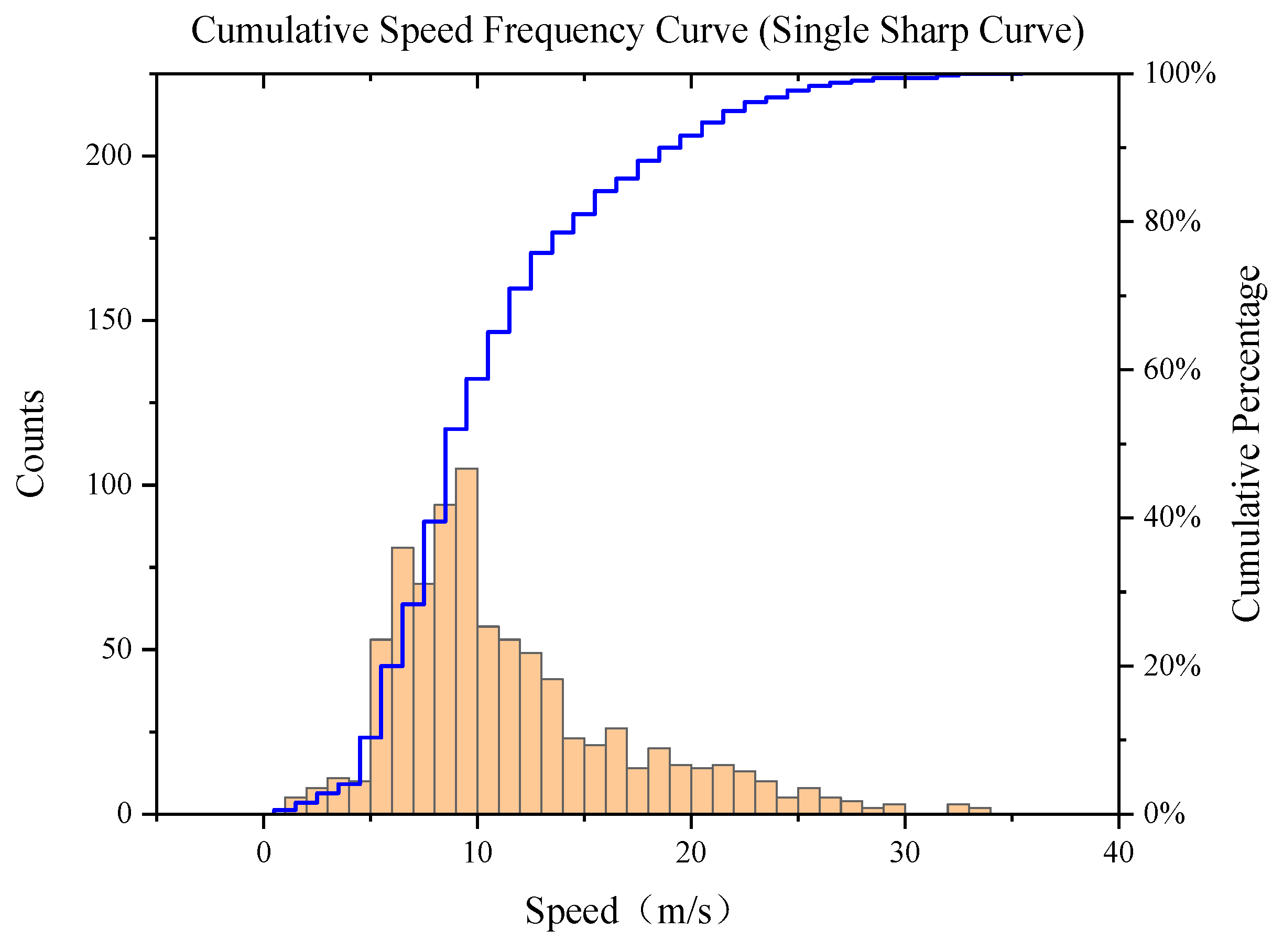
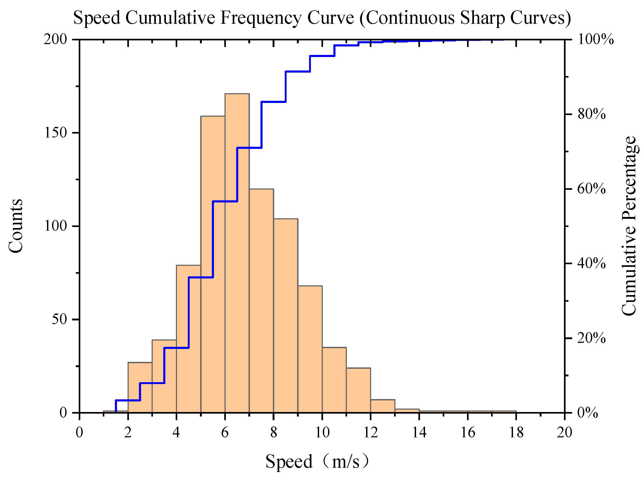
To more intuitively illustrate the differences in vehicle speed between single-curve and continuous-curve road segments, we plotted cumulative frequency distribution diagrams of acceleration and speed (see Figure 1, Figure 2, Figure 3 and Figure 4). In the figures, the blue curve represents the cumulative frequency of the current samples, while the orange histogram indicates the number of samples within each interval. The distribution characteristics in the figure clearly show that the acceleration distribution for a single curve is widespread, with a large range, whereas the acceleration for continuous curves is more concentrated, with a smaller range. Similarly, the speed distribution for a single curve is also wide, with a large range, while the speed for continuous curves is more concentrated, with a smaller range. The vehicle speed and acceleration on single curves are significantly higher than those on continuous curves. This indicates that the type of curve has a significant impact on vehicle dynamics. Roads with single curves typically allow vehicles to maintain higher speeds and accelerations, while roads with continuous curves force vehicles to reduce speed to ensure safety.

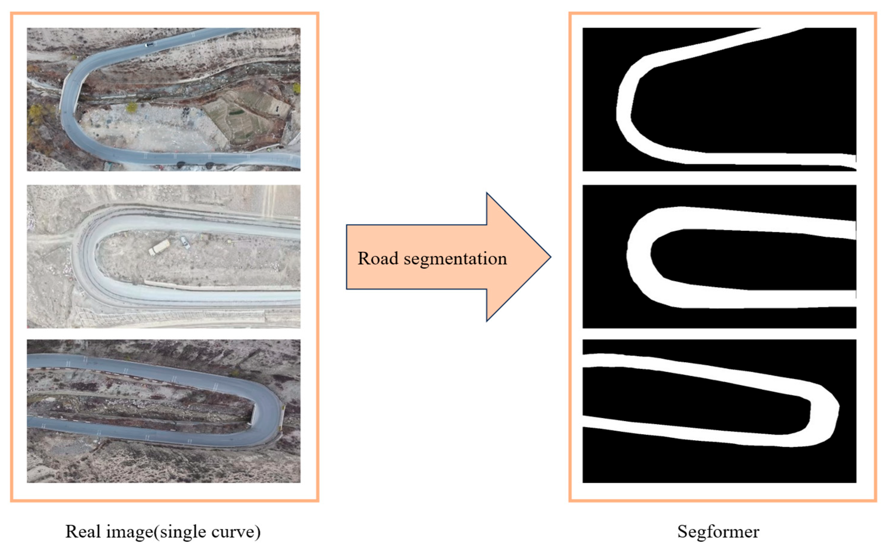
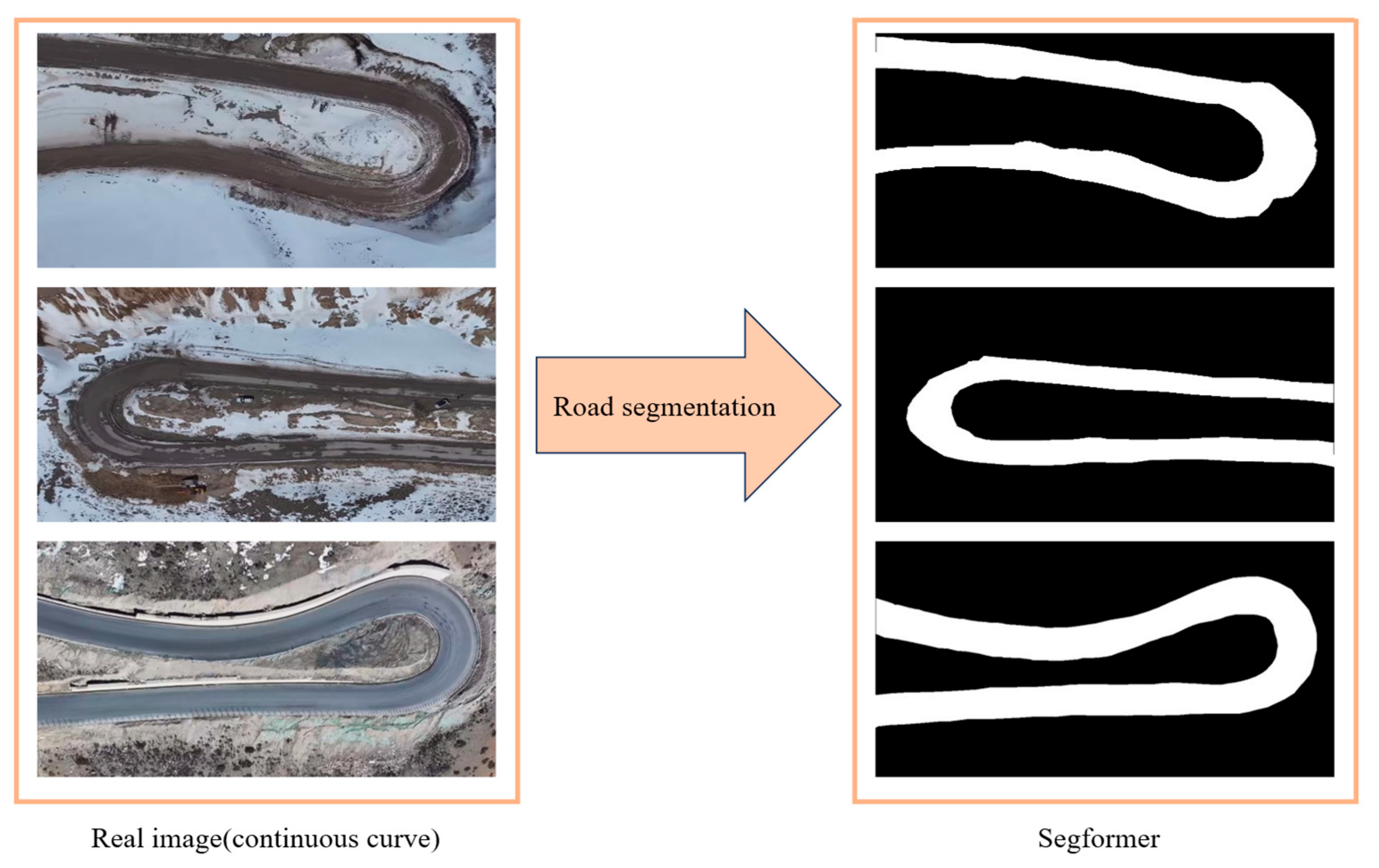
This study uses the Segformer image segmentation method to determine the curvature radius of sharp curves in high-altitude mountainous highways. The specific steps are as follows:

• Road Segmentation: Use Segformer to segment the road image and separate the road from the background.
• Import to CAD Software: Import the segmented image into CAD software.
• Spline Curve Fitting: Use spline curve fitting to obtain a smooth representation of the road centerline.
• Polyline Fitting: Break the fitted spline curve into segments and convert it into a polyline.
• Curvature Radius Calculation: Use the annotation function in CAD software to calculate the curvature radius of the road.

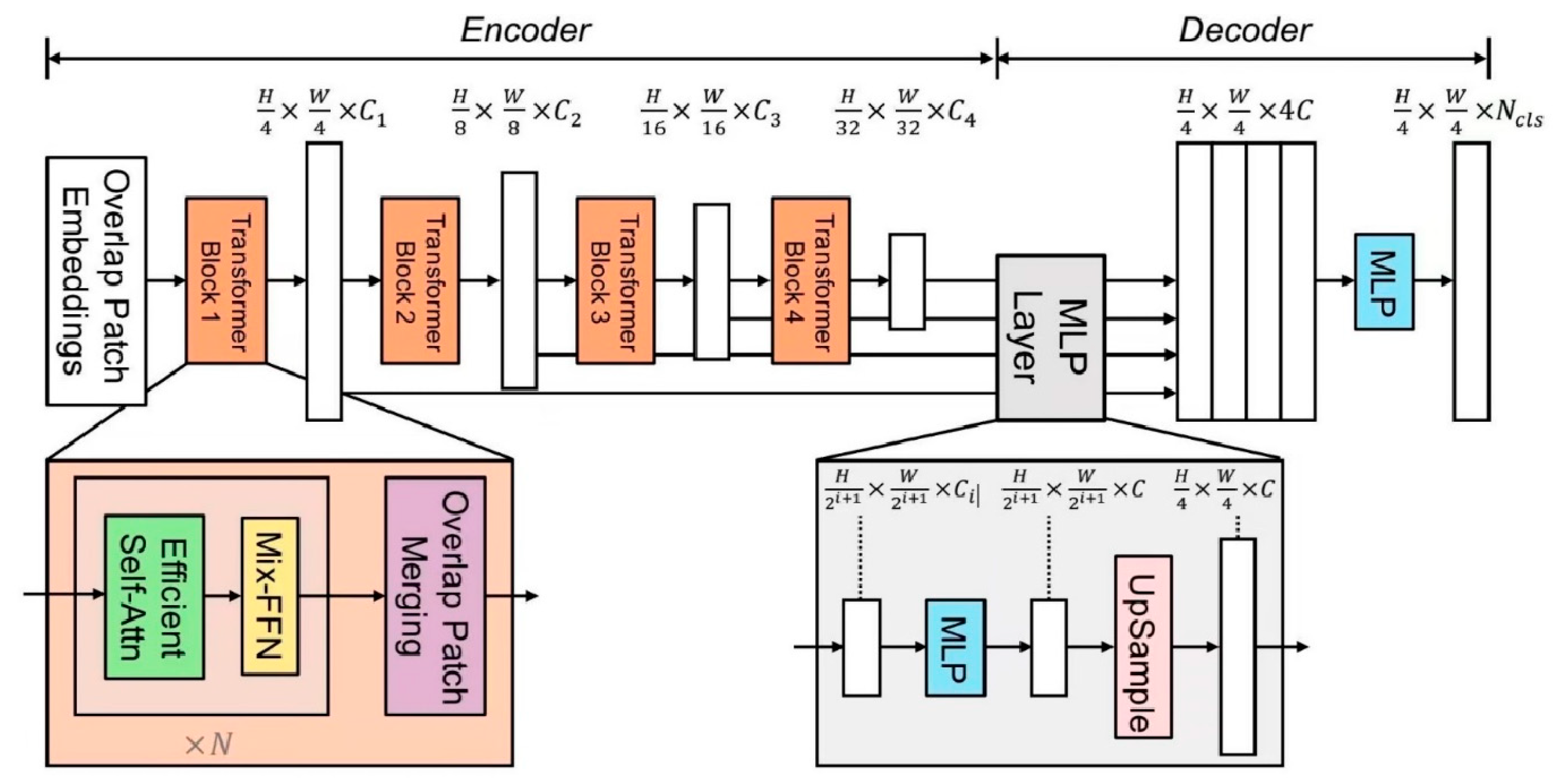
SegFormer is an efficient image segmentation model based on the Transformer architecture. Compared with CNN-based models such as U-Net, it demonstrates superior performance in complex scenarios, such as traffic environments. It utilizes multi-scale feature fusion and a lightweight design, ensuring high accuracy while reducing computational costs. In this study, Segformer is applied to the road segmentation task. The specific hyperparameter settings are shown in

Table 4. Segformer hyperparameter settings.

Hyperparameterization	Set Value
keys	values
num_classes	2
input_shape	[512, 512]
Init_Epoch	0
Freeze_Epoch	50
UnFreeze_Epoch	300
Freeze_batch_size	8
Unfreeze_batch_size	16
Freeze_Train	FALSE
Init_lr	0.0001
Min_lr	1.00 × 10−6
optimizer_type	adamw
momentum	0.9
lr_decay_type	cos
save_period	5
save_dir	logs
num_workers	4
num_train	4980
num_val	1246

, and the model architecture is illustrated in Figure 5. The results of the image segmentation are displayed in Figure 6 and Figure 7.

3.2. Overview of Base Learners

(1) Bi-LSTM

Bidirectional Long Short-Term Memory (Bi-LSTM) is a variant of LSTM, which is a type of Recurrent Neural Network (RNN) that combines both forward and backward LSTM layers. This structure allows it to capture bidirectional dependencies in time series data [37,38].

(2) Informer

The core of the Transformer model is the self-attention mechanism, which captures long-range dependencies within a sequence, overcoming the limitations of RNNs and CNNs when processing long sequences. The Transformer consists of an encoder and a decoder, with each layer of both the encoder and decoder containing multi-head attention mechanisms and feedforward neural networks. Additionally, positional encoding is used to inject positional information into the sequence [39]. However, when the sequence is very long, the self-attention mechanism in the Transformer results in high computational complexity, consuming a significant amount of computational resources and time. To address the challenges of high computational complexity and inefficiency in long sequence prediction, the Informer model was proposed. This model introduces the ProbSparse self-attention mechanism to reduce computational load, utilizes self-attention distillation to decrease memory consumption, and adopts a generative decoder to speed up the prediction process. These improvements make Informer more efficient and more effective than the traditional Transformer model when handling long-sequence time series prediction tasks [40].

Disregarding computational overhead, the Informer also outperforms the Transformer in this study. A small comparative experiment was conducted: when using a single-curve multi-source heterogeneous dataset, the Transformer achieved an MSE of 8.0214, while the Informer achieved an MSE of 7.2147; when using a continuous-curve multi-source heterogeneous dataset, the Transformer achieved an MSE of 2.6053, whereas the Informer achieved an MSE of 2.4690. Therefore, when selecting a base learner with an attention mechanism, we adopted the superior Informer model rather than the Transformer model.

(3) GRU

The Gated Recurrent Unit (GRU) is a variant of Long Short-Term Memory (LSTM). The GRU introduces the update gate and reset gate, which simplify the LSTM structure and significantly improve computational efficiency [41].

In summary, we selected three base learners, Bi-LSTM, Informer, and GRU, each representing a distinct modeling principle. Bi-LSTM embodies the bidirectional principle, capable of capturing both historical and future data; Informer represents mainstream attention mechanism models; and GRU represents a simplified architecture that balances efficiency and high performance.

3.3. Dynamic Weight Allocation Method

The stacking ensemble learning model first sets up multiple base learners and concatenates their output results to form a meta-dataset. A meta-learner is then used to learn from the meta-dataset, ultimately producing the output result. The results of the stacking ensemble learning model are shown in Figure 8.

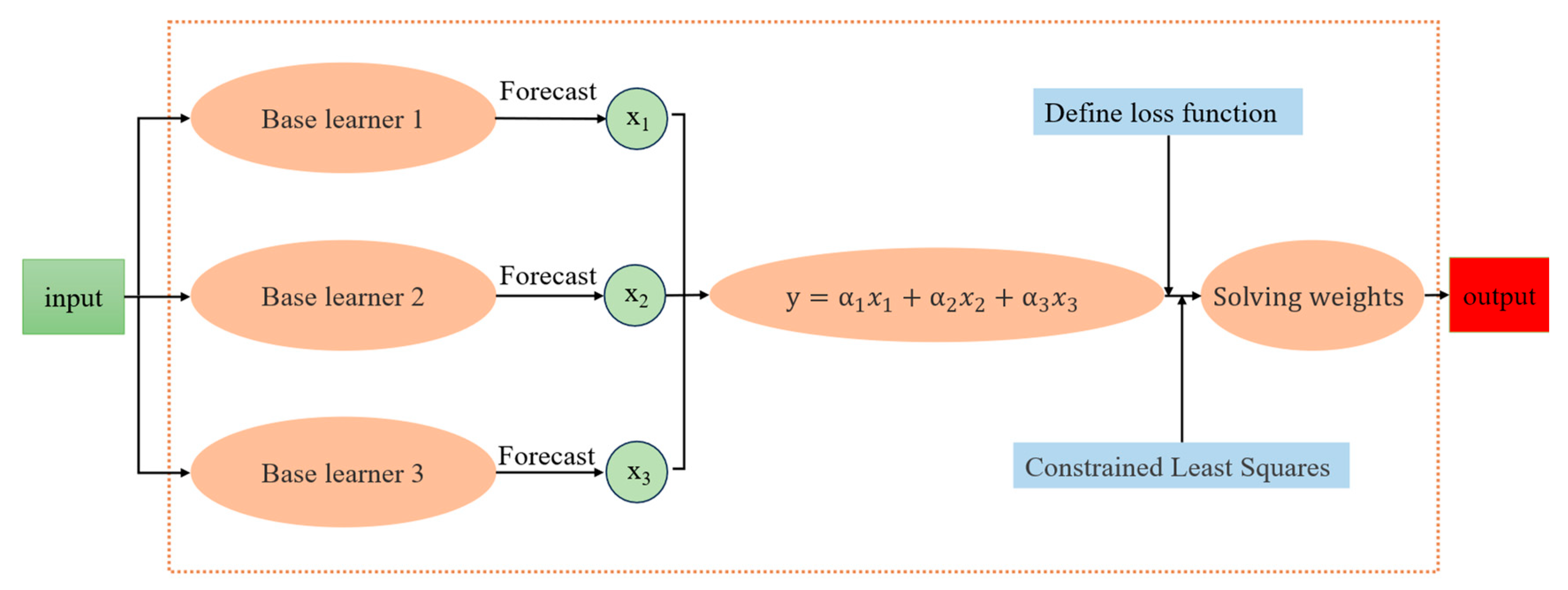
The dynamic weight allocation method proposed in this study retains the output results of multiple base learners and assigns weights to them. A new loss function is defined as the mean squared error of the linear weighted sum of the true values and the output results. Based on the loss function, weighted outputs are determined by using constrained least squares, variable substitution, and solving the weights using the normal equation. Finally, the linear weighted sum of the output results is taken as the final output. The structure of the dynamic weight allocation model proposed in this study is shown in Figure 9.

The dynamic weight allocation algorithm is as follows:

Define the loss function L:

$$\mathrm{L}={\displaystyle \frac{1}{\mathrm{n}}}{\displaystyle \sum _{\mathrm{i}}^{\mathrm{n}}{\left({\mathrm{y}}_{\mathrm{i}}-{\mathrm{\alpha }}_1{\mathrm{x}}_{1\mathrm{i}}-{\mathrm{\alpha }}_2{\mathrm{x}}_{2\mathrm{i}}-{\mathrm{\alpha }}_3{\mathrm{x}}_{3\mathrm{i}}\right)}^2}$$

(3)

where ${\mathrm{y}}_{\mathrm{i}}$ denotes the true value; ${\mathrm{\alpha }}_1$ denotes the weight given to the prediction result of the first base learner; ${\mathrm{\alpha }}_2$ denotes the weight given to the prediction result of the second base learner; ${\mathrm{\alpha }}_3$ denotes the weight given to the prediction result of the third base learner; ${\mathrm{x}}_{1\mathrm{i}}$ denotes the prediction result of the first base learner; ${\mathrm{x}}_{2\mathrm{i}}$ denotes the prediction result of the second base learner; and ${\mathrm{x}}_{3\mathrm{i}}$ denotes the prediction result of the third base learner’s prediction result.

Weight normalization constraint:

$${\mathrm{\alpha }}_1+{\mathrm{\alpha }}_2+{\mathrm{\alpha }}_3=1$$

(4)

Variable substitution:

Eliminate the weight variable ${\mathrm{\alpha }}_3$ through the constraint condition:

$${\mathrm{\alpha }}_3=1-{\mathrm{\alpha }}_1-{\mathrm{\alpha }}_2$$

(5)

Substitute it into the loss function, L:

$$\mathrm{L}={\displaystyle \frac{1}{\mathrm{n}}}{\displaystyle \sum _{\mathrm{i}}^{\mathrm{n}}{\left({\mathrm{y}}_{\mathrm{i}}-{\mathrm{\alpha }}_1{\mathrm{x}}_{1\mathrm{i}}-{\mathrm{\alpha }}_2{\mathrm{x}}_{2\mathrm{i}}-\left(1-{\mathrm{\alpha }}_1-{\mathrm{\alpha }}_2\right){\mathrm{x}}_{3\mathrm{i}}\right)}^2}$$

(6)

Assume that

$${{\mathrm{y}}^{\prime }}_{\mathrm{i}}={\mathrm{y}}_{\mathrm{i}}-{\mathrm{x}}_{3\mathrm{i}}$$

(7)

$${\mathrm{z}}_{1\mathrm{i}}={\mathrm{x}}_{1\mathrm{i}}-{\mathrm{x}}_{3\mathrm{i}}$$

(8)

$${\mathrm{z}}_{2\mathrm{i}}={\mathrm{x}}_{2\mathrm{i}}-{\mathrm{x}}_{3\mathrm{i}}$$

(9)

Substitute them into the loss function, L:

$$\mathrm{L}={\displaystyle \frac{1}{\mathrm{n}}}{\displaystyle \sum _{\mathrm{i}}^{\mathrm{n}}{\left({{\mathrm{y}}^{\prime }}_{\mathrm{i}}-{\mathrm{\alpha }}_1{\mathrm{z}}_{1\mathrm{i}}-{\mathrm{\alpha }}_2{\mathrm{z}}_{2\mathrm{i}}\right)}^2}$$

(10)

After variable substitution, the constrained problem is successfully transformed into an unconstrained problem.

Construct the design matrix, X; response vector, Y; and parameter vector α:

$$\mathrm{X}=\left[\begin{array}{cc}{\mathrm{z}}_{11}& {\mathrm{z}}_{21}\\ {\mathrm{z}}_{12}& {\mathrm{z}}_{22}\\ ⋮& ⋮\\ {\mathrm{z}}_{1\mathrm{n}}& {\mathrm{z}}_{2\mathrm{n}}\end{array}\right]$$

(11)

$$\mathrm{Y}=\left[\begin{array}{c}{{\mathrm{y}}^{\prime }}_1\\ {{\mathrm{y}}^{\prime }}_2\\ ⋮\\ {{\mathrm{y}}^{\prime }}_{\mathrm{n}}\end{array}\right]$$

(12)

$$\mathrm{\alpha }=\left[\begin{array}{c}{\mathrm{\alpha }}_1\\ {\mathrm{\alpha }}_2\end{array}\right]$$

(13)

Solve for the weights using the normal equation:

$$\mathrm{\alpha }={\left({\mathrm{X}}^{\mathrm{T}}\mathrm{X}\right)}^{-1}{\mathrm{X}}^{\mathrm{T}}\mathrm{Y}$$

(14)

The optimal weight coefficients for each base learner are

$${\mathrm{\alpha }}_1={\left({\mathrm{X}}^{\mathrm{T}}\mathrm{X}\right)}_{1,1}^{-1}{\left({\mathrm{X}}^{\mathrm{T}}\mathrm{Y}\right)}_1+{\left({\mathrm{X}}^{\mathrm{T}}\mathrm{X}\right)}_{1,2}^{-1}{\left({\mathrm{X}}^{\mathrm{T}}\mathrm{Y}\right)}_2$$

(15)

$${\mathrm{\alpha }}_2={\left({\mathrm{X}}^{\mathrm{T}}\mathrm{X}\right)}_{2,1}^{-1}{\left({\mathrm{X}}^{\mathrm{T}}\mathrm{Y}\right)}_1+{\left({\mathrm{X}}^{\mathrm{T}}\mathrm{X}\right)}_{2,2}^{-1}{\left({\mathrm{X}}^{\mathrm{T}}\mathrm{Y}\right)}_2$$

(16)

$${\mathrm{\alpha }}_3=1-{\mathrm{\alpha }}_1-{\mathrm{\alpha }}_2$$

(17)

The optimal prediction result is

$${\widehat{\mathrm{y}}}_{\mathrm{i}}={\mathrm{\alpha }}_1{\mathrm{x}}_{1\mathrm{i}}+{\mathrm{\alpha }}_2{\mathrm{x}}_{2\mathrm{i}}+{\mathrm{\alpha }}_3{\mathrm{x}}_{3\mathrm{i}}$$

(18)

4. Model Comparison and Engineering Application

4.1. Model Comparison

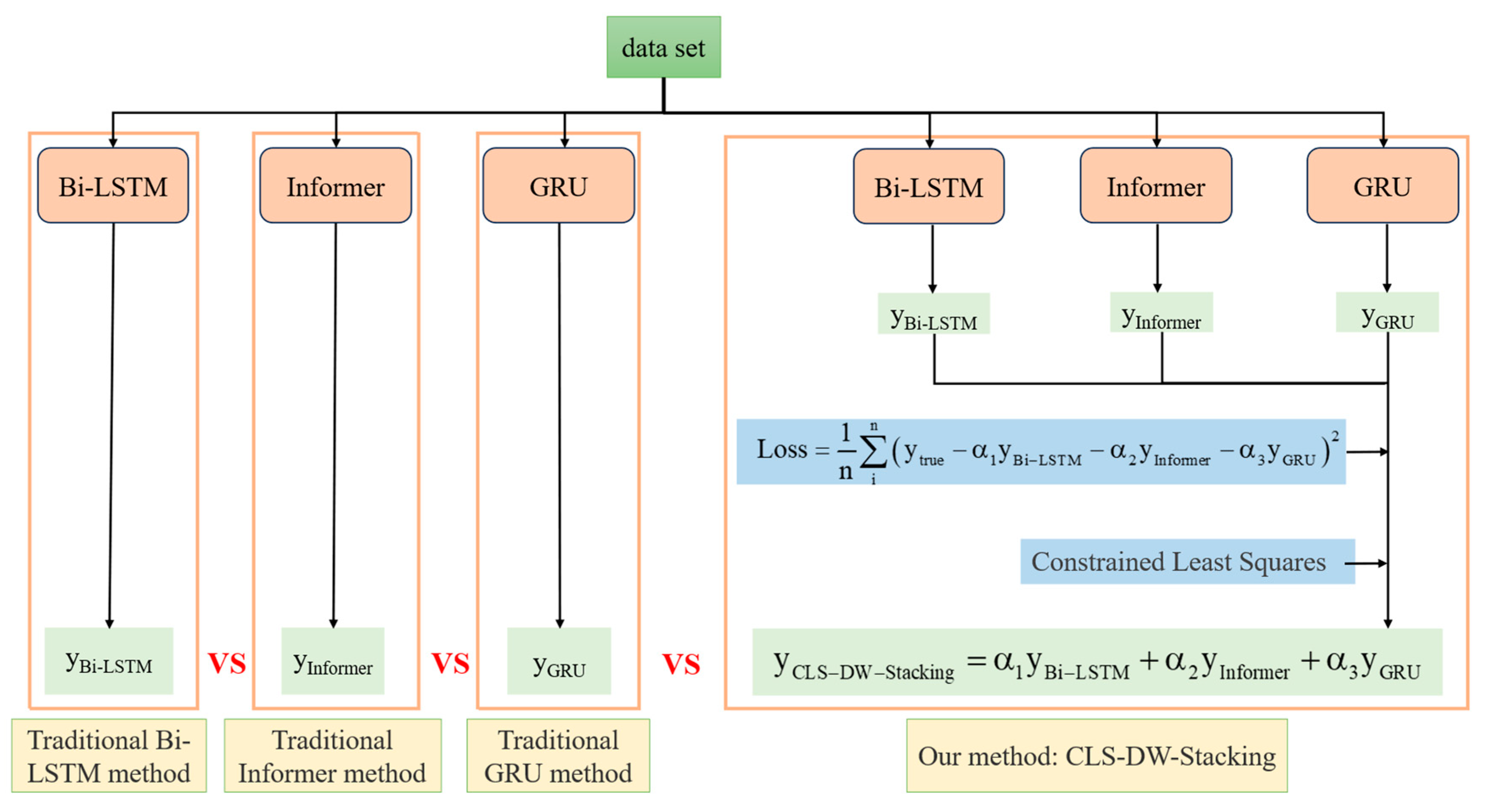
A common and widely used approach is using a single deep learning method (such as Bi-LSTM, Informer, or GRU) for speed prediction. However, the CLS-DW Stacking method proposed in this study is essentially a new ensemble framework that integrates multiple deep learning methods for prediction. To validate the superior prediction performance of the proposed CLS-DW Stacking speed prediction model, a comparative experiment was designed and conducted. In the experiment, traditional time series prediction models, including Bi-LSTM, Informer, and GRU, were selected for comparison with the CLS-DW Stacking model proposed in this study, highlighting the advantages of the proposed model. Specifically, four experimental groups were set up: Experiment Group 1 represents the traditional method Bi-LSTM, Experiment Group 2 represents the traditional method Informer, Experiment Group 3 represents the traditional method GRU, and Experiment Group 4 represents the CLS-DW Stacking method proposed in this study. In this comparison experiment, the only variable is the model. The four experimental groups were trained using the same training set, and the performance of the models was tested on the same testing set. The specific experimental setups are shown in Figure 10.

Before training the model, data preprocessing is required for the single sharp curve road multi-source heterogeneous dataset and the continuous sharp curve road multi-source heterogeneous dataset to standardize feature scales and prevent overfitting. In this study, the raw datasets are standardized, and the specific calculation method is shown in Equation (19).

$${\mathrm{x}}_{\mathrm{s}\mathrm{t}\mathrm{d}}={\displaystyle \frac{\mathrm{x}-\mathrm{\mu }}{\mathrm{\sigma }}}$$

(19)

where ${\mathrm{x}}_{\mathrm{s}\mathrm{t}\mathrm{d}}$ is the normalized feature; $\mathrm{x}$ is the original feature; $\mathrm{u}$ is the mean of the feature; and $\mathrm{\sigma }$ is the standard deviation of the feature.

In both the single-curve road multi-source heterogeneous dataset and the continuous-curve road multi-source heterogeneous dataset, three base learners—Bi-LSTM, Informer, and GRU—were used for training. Through multiple experiments, the models were ensured to converge without overfitting, and the corresponding hyperparameters were recorded. The hyperparameter settings for the three base learners are presented in

Table 5. Three kinds of superparameter settings for base learners.

	Bi-LSTM	Informer	GRU
epoch	1000	1500	1000
hidden_size	64	64	64
learning_rate	Adam (0.01)	Adam (0.001)	Adam (0.01)
num_layers	1	3	2
head	\	8	\

, and the training losses are shown in Figure 11 and Figure 12.

The proposed CLS-DW Stacking method in this study essentially integrates the three aforementioned base learners. To ensure the robustness of the ensemble method, it is first necessary to verify the stability of the individual base learners. In this study, 3-fold cross-validation was employed to evaluate the stability of the three base learners, and the results are presented in

Table 6. Cross-validation results of the three base learners.

	Single Curve Dataset			Continuous Curve Dataset
	Bi-LSTM	Informer	GRU	Bi-LSTM	Informer	GRU
Fold 1 (MSE)	12.3755	6.619	8.9291	4.9436	2.0064	2.6593
Fold 2 (MSE)	13.0064	6.611	9.1949	4.4413	2.96	3.4135
Fold 3 (MSE)	12.9832	5.1633	8.6642	4.4122	2.0979	2.2975
Mean	12.7884	6.1311	8.9294	4.5991	2.3548	2.7901
Standard Deviation	0.2921	0.6844	0.2167	0.2439	0.4296	0.4649

.

According to the cross-validation results shown in Table 6, the three base learners exhibited relatively robust performance on both datasets used in this study, confirming their suitability for inclusion in the proposed ensemble method.

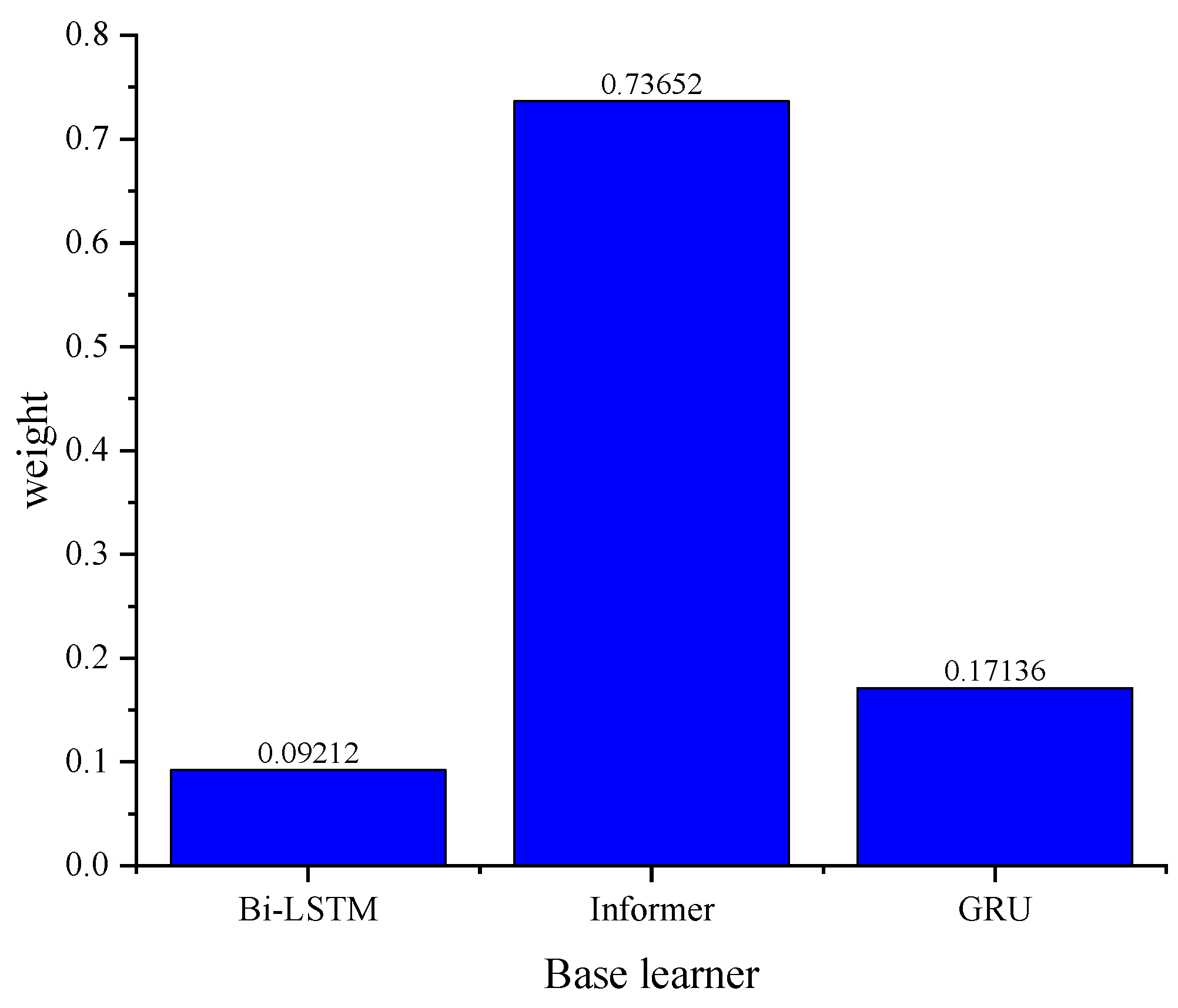
According to the dynamic weight allocation method, weights are assigned to the three base learners, Bi-LSTM, Informer, and GRU. The weight allocation is shown in Figure 13.

In order to compare the performance of the models, we evaluate the three base learners and the dynamic weight allocation multi-model stacking method proposed in this study on the test set. The evaluation metrics include the mean squared error (MSE), Root Mean Squared Error (RMSE), Mean Absolute Error (MAE), and Coefficient of Determination (R²). Here, R² represents the degree to which the independent variables explain the variation in the dependent variable, i.e., the proportion of the total variation in the dependent variable that is explained by the independent variables in the model. The specific calculation methods for the metrics are shown in Equations (20)–(23). The comparison results are shown in

Table 7. Model comparison table.

	Single Curve Dataset				Continuous Curve Dataset
	Bi-LSTM	Informer	GRU	Ours	Bi-LSTM	Informer	GRU	Ours
MSE	11.8700	7.2147	10.3826	7.0753	5.5917	2.4690	2.5521	2.2793
RMSE	3.4453	2.6860	3.2222	2.6599	2.3647	1.5713	1.5975	1.5097
MAE	2.1711	1.5792	1.9995	1.5652	1.6174	0.9547	1.1408	0.9610
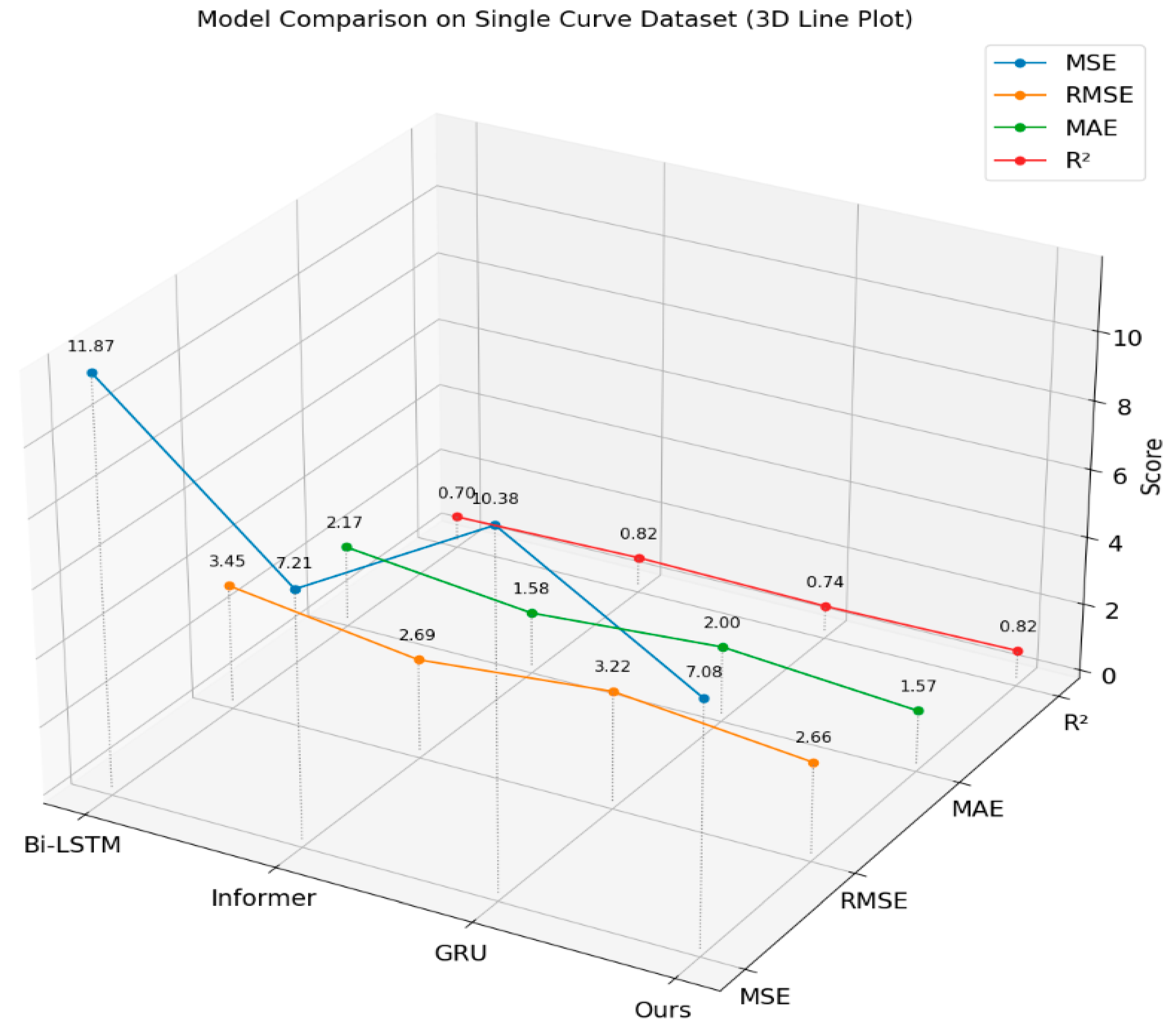
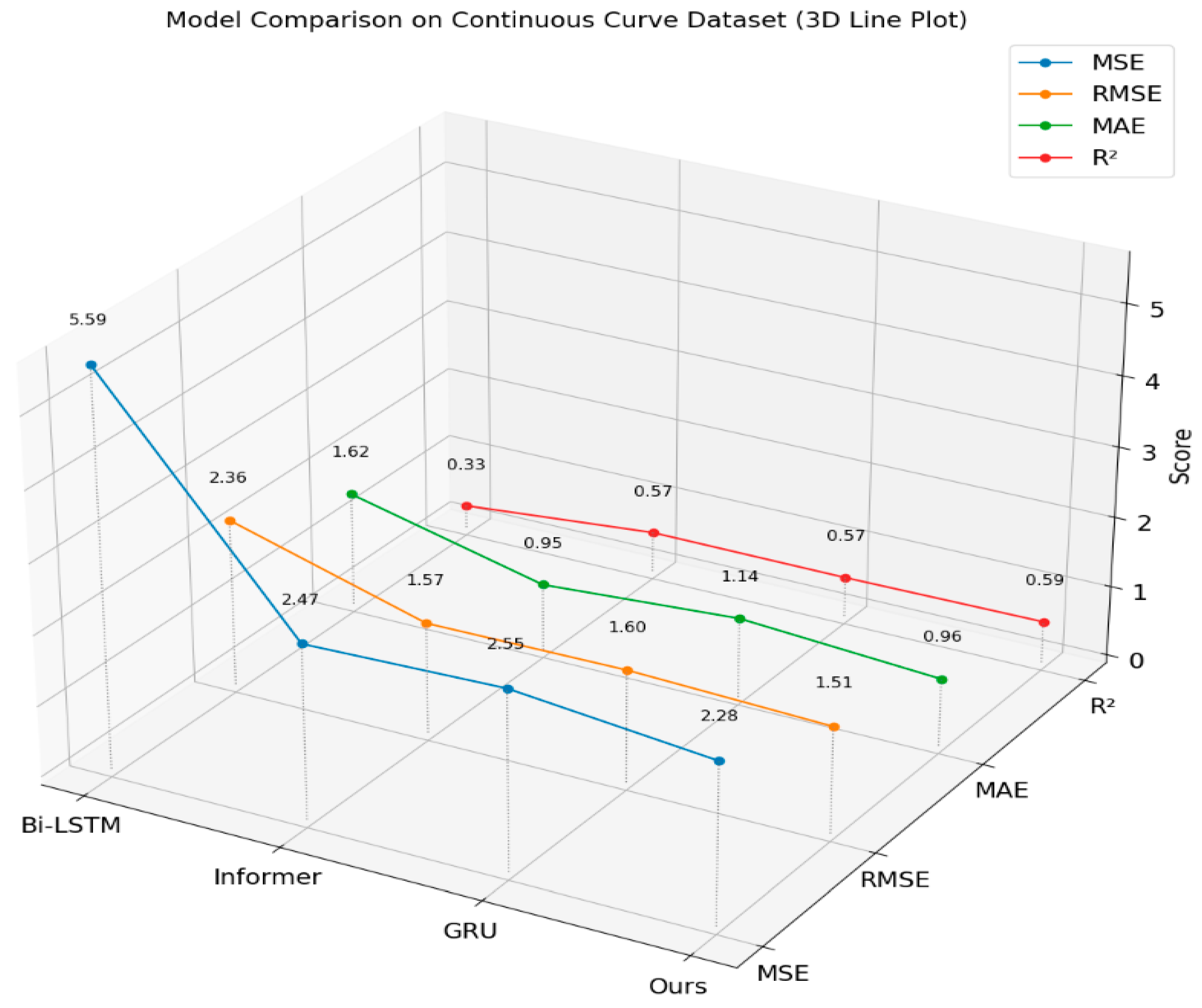
R2	0.7042	0.8206	0.7420	0.8212	0.3261	0.5740	0.5686	0.5936

. The comparative visualization results are shown in Figure 14 and Figure 15.

$$\mathrm{M}\mathrm{S}\mathrm{E}={\displaystyle \frac{1}{\mathrm{n}}}{\displaystyle \sum _{\mathrm{i}=1}^{\mathrm{n}}{\left({\mathrm{y}}_{\mathrm{i}}-{\widehat{\mathrm{y}}}_{\mathrm{i}}\right)}^2}$$

(20)

$$\mathrm{R}\mathrm{M}\mathrm{S}\mathrm{E}=\sqrt{{\displaystyle \frac{1}{\mathrm{n}}}{\displaystyle \sum _{\mathrm{i}=1}^{\mathrm{n}}{\left({\mathrm{y}}_{\mathrm{i}}-{\widehat{\mathrm{y}}}_{\mathrm{i}}\right)}^2}}$$

(21)

$$\mathrm{M}\mathrm{A}\mathrm{E}={\displaystyle \frac{1}{\mathrm{n}}}{\displaystyle \sum _{\mathrm{i}=1}^{\mathrm{n}}\left|{\mathrm{y}}_{\mathrm{i}}-{\widehat{\mathrm{y}}}_{\mathrm{i}}\right|}$$

(22)

$${\mathrm{R}}^2=1-{\displaystyle \frac{{\displaystyle \sum _{\mathrm{i}=1}^{\mathrm{n}}{\left({\mathrm{y}}_{\mathrm{i}}-{\widehat{\mathrm{y}}}_{\mathrm{i}}\right)}^2}}{{\displaystyle \sum _{\mathrm{i}=1}^{\mathrm{n}}{\left({\mathrm{y}}_{\mathrm{i}}-\overline{\mathrm{y}}\right)}^2}}}$$

(23)

where ${\mathrm{y}}_{\mathrm{i}}$ is the true value; ${\widehat{\mathrm{y}}}_{\mathrm{i}}$ is the model-predicted value; and ${\overline{\mathrm{y}}}_{\mathrm{i}}$ is the average of the true values.

In the prediction results of the single sharp curve road dataset, the CLS-DW Stacking model outperforms the others in all of the MSE, RMSE, and MAE metrics, with values of 7.0753, 2.6599, and 1.5652, respectively, and an R² value of 0.8212. This indicates that the model effectively balances prediction accuracy and data fitting. In contrast, the Bi-LSTM, Informer, and GRU models perform slightly worse on the MSE, RMSE, and MAE metrics, with their R² values also being slightly lower.

For the continuous sharp curve road dataset, the CLS-DW Stacking model also achieves the best results in MSE and RMSE, with values of 2.2793 and 1.5097, respectively, and an R² value of 0.5936. Although it slightly underperforms compared to the Informer model in terms of the MAE, the CLS-DW Stacking model demonstrates its applicability and stability across different road types.

Overall, the CLS-DW Stacking model outperforms single deep learning models on both the single sharp curve and continuous sharp curve road datasets, exhibiting better predictive performance and generalization ability. Comparative experiments further reveal that all models exhibit significantly lower prediction errors on the continuous curve multi-source heterogeneous dataset than on the single curve dataset. The underlying reason is that vehicle speed ranges in continuous curves are narrower, and the data distribution is more concentrated, which substantially reduces model uncertainty. This enables the models to more effectively capture robust patterns, thereby improving overall prediction accuracy.

4.2. Engineering Applications

Currently, there are no relevant standards for speed limits on sharp-curved roads in plateau mountainous areas. In order to provide a basis for policy formulation by relevant departments, this study uses the CLS-DW Stacking model to predict speeds on sharp-curved roads under different conditions.

In the prediction, it is assumed that there are no oncoming or following vehicles, and the vehicle is driving normally along the road centerline in an ideal situation where acceleration is zero. The influence of vehicle type, slope, curvature change rate (CCR), and altitude is considered.

Only two vehicle types are considered (because there are few non-motorized vehicles and light trucks on National Highway G318): a standard vehicle (denoted by 2) and a large truck (denoted by 4). Three slope conditions are considered: no slope (0), downhill (−0.05), and uphill (0.05). The curvature change rate is considered under two conditions: when entering or exiting a curve (1) and when in the middle of a curve (0.2). Four altitude conditions are considered: 2000 m, 3000 m, 4000 m, and 5000 m. The prediction results are shown in

Table 8. Predicted values of single curve speed.

Motorcycle Type	Slope	Curvature Change Rate	Altitude	Speed (m/s)
2	0	1	2000	24.8031
2	0.05	1	2000	25.5595
2	−0.05	1	2000	23.4495
2	0	0.2	2000	23.4394
2	0.05	0.2	2000	24.0647
2	−0.05	0.2	2000	22.6756
2	0	1	3000	19.8675
2	0.05	1	3000	19.7075
2	−0.05	1	3000	26.5565
2	0	0.2	3000	15.2135
2	0.05	0.2	3000	15.3725
2	−0.05	0.2	3000	8.1842
2	0	1	4000	14.9069
2	0.05	1	4000	13.7794
2	−0.05	1	4000	13.9432
2	0	0.2	4000	14.8654
2	0.05	0.2	4000	14.2786
2	−0.05	0.2	4000	13.9718
2	0	1	5000	14.9926
2	0.05	1	5000	14.9220
2	−0.05	1	5000	14.4207
2	0	0.2	5000	15.0972
2	0.05	0.2	5000	15.0585
2	−0.05	0.2	5000	14.4071
4	0	1	2000	15.5127
4	0.05	1	2000	16.0471
4	−0.05	1	2000	15.0898
4	0	0.2	2000	15.3845
4	0.05	0.2	2000	15.1380
4	−0.05	0.2	2000	14.1080
4	0	1	3000	10.4234
4	0.05	1	3000	10.3304
4	−0.05	1	3000	8.4337
4	0	0.2	3000	7.6489
4	0.05	0.2	3000	9.4065
4	−0.05	0.2	3000	7.6326
4	0	1	4000	11.6198
4	0.05	1	4000	11.1926
4	−0.05	1	4000	10.8585
4	0	0.2	4000	11.6492
4	0.05	0.2	4000	10.9067
4	−0.05	0.2	4000	10.7321
4	0	1	5000	14.7449
4	0.05	1	5000	14.5877
4	−0.05	1	5000	15.0818
4	0	0.2	5000	14.8656
4	0.05	0.2	5000	14.4558
4	−0.05	0.2	5000	14.9372

and

Table 9. Predicted values of continuous curve speed.

Motorcycle Type	Slope	Curvature Change Rate	Altitude	Speed (m/s)
2	0	1	2000	6.6566
2	0.05	1	2000	6.8118
2	−0.05	1	2000	6.4940
2	0	0.2	2000	6.7299
2	0.05	0.2	2000	6.8719
2	−0.05	0.2	2000	6.8048
2	0	1	3000	6.9173
2	0.05	1	3000	7.1457
2	−0.05	1	3000	6.6485
2	0	0.2	3000	6.9568
2	0.05	0.2	3000	6.8668
2	−0.05	0.2	3000	7.2836
2	0	1	4000	7.1608
2	0.05	1	4000	8.0792
2	−0.05	1	4000	7.2099
2	0	0.2	4000	6.8518
2	0.05	0.2	4000	7.5434
2	−0.05	0.2	4000	7.2820
2	0	1	5000	7.2887
2	0.05	1	5000	7.7674
2	−0.05	1	5000	6.1940
2	0	0.2	5000	8.0748
2	0.05	0.2	5000	7.0249
2	−0.05	0.2	5000	7.6651
4	0	1	2000	7.1372
4	0.05	1	2000	6.6863
4	−0.05	1	2000	7.0727
4	0	0.2	2000	7.0611
4	0.05	0.2	2000	6.8403
4	−0.05	0.2	2000	7.5267
4	0	1	3000	6.9385
4	0.05	1	3000	7.3007
4	−0.05	1	3000	7.3045
4	0	0.2	3000	6.6109
4	0.05	0.2	3000	6.7209
4	−0.05	0.2	3000	7.9342
4	0	1	4000	7.1777
4	0.05	1	4000	8.1492
4	−0.05	1	4000	7.5146
4	0	0.2	4000	6.3897
4	0.05	0.2	4000	6.8382
4	−0.05	0.2	4000	5.6042
4	0	1	5000	5.3585
4	0.05	1	5000	5.2500
4	−0.05	1	5000	4.6871
4	0	0.2	5000	4.7412
4	0.05	0.2	5000	5.0542
4	−0.05	0.2	5000	6.7165

.

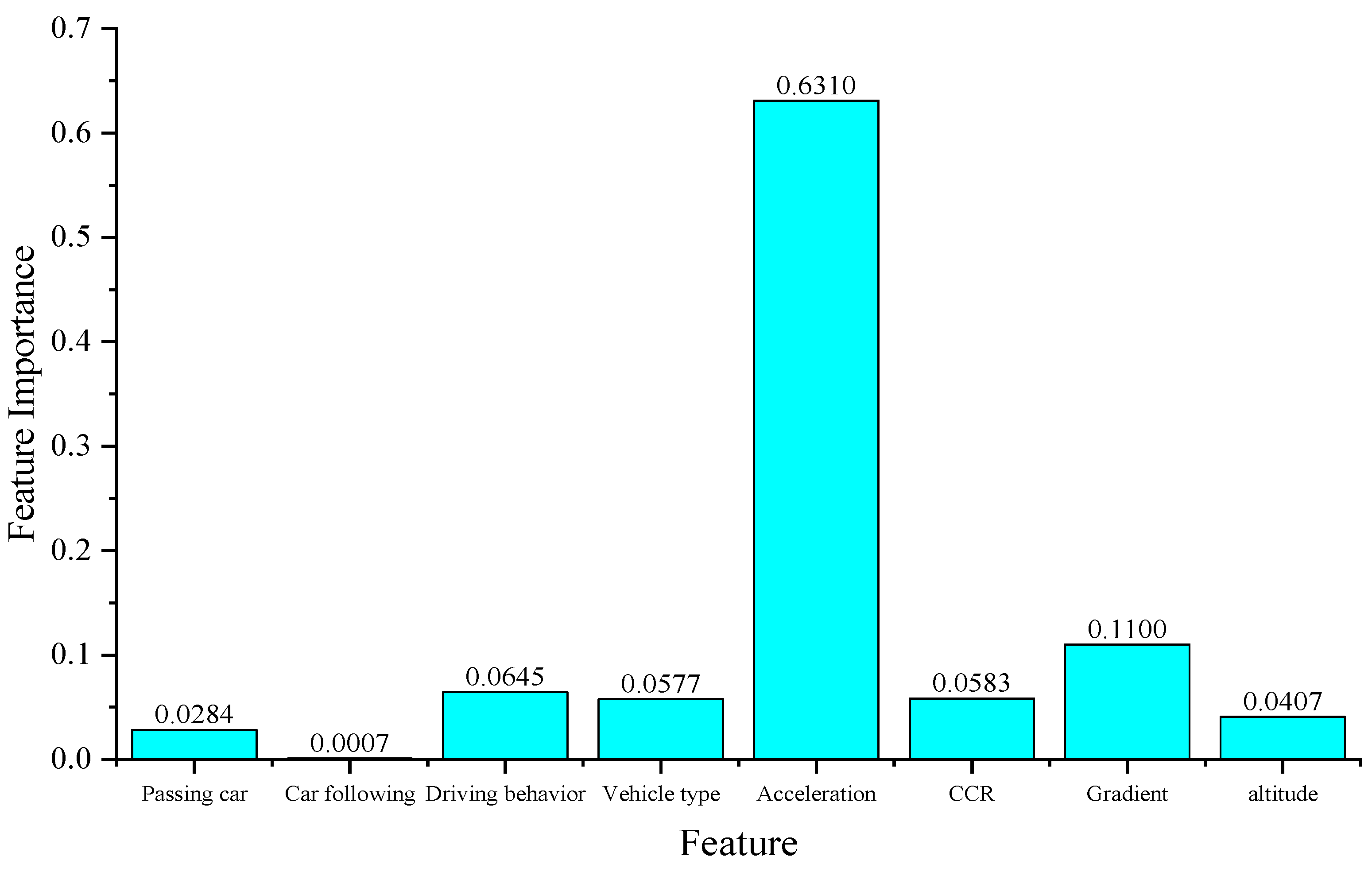
Although the proposed model successfully generates vehicle speed predictions that can assist relevant authorities in formulating speed limit policies, the interpretability of these predictions remains limited. To enhance the practical applicability of the model, this study further introduces an interpretable decision tree model to evaluate the importance of each feature variable. This approach provides more targeted and evidence-based guidance for policymakers. The feature importance results for the single-curve and continuous-curve road scenarios are illustrated in Figure 16 and Figure 17, respectively.

5. Conclusions and Future Work

Sharp-curved roads in plateau mountainous areas are characterized by unique geographical environments, road structures, and natural conditions, which result in traffic environments that differ from those of plain roads. In this study, based on the characteristics of sharp-curved roads in plateau mountainous areas, both single curves and continuous curves are considered, and the CLS-DW Stacking model is proposed for speed prediction. The prediction results are expected to provide data for relevant departments to support the improvement in speed limit policies.

From the single-curve speed prediction results, the following conclusions can be drawn:

• Effect of Vehicle Type on Speed:
  It has been observed that standard vehicles generally travel at higher speeds than large trucks across different altitudes. At lower altitudes (e.g., 2000 m), a speed of approximately 23 m/s is recorded for standard vehicles, whereas a speed of about 15 m/s is recorded for large trucks, indicating a significant difference between the two vehicle types.
• Effect of Slope on Speed:
  At an altitude of 3000 m, the slope is found to exert a significant impact on the speeds of both standard vehicles and large trucks. However, at other altitudes, the influence of slope on speed is comparatively minor.
• Effect of Curvature Change Rate on Speed:
  Vehicle speeds are generally higher when entering or exiting a curve than when positioned at the midpoint of the curve, although certain exceptions have been noted.
• Effect of Altitude on Speed:
  A significant effect of increasing altitude on vehicle speed has been identified. For standard vehicles, speed is observed to gradually decrease with altitude, with a rapid decline occurring above 3000 m. Large trucks display a similar trend, though the magnitude of speed change is less pronounced compared to that of standard vehicles.

From the continuous curve speed prediction results, the following conclusions can be drawn:

• Effect of Vehicle Type on Speed:
  The speed prediction results for standard vehicles and large trucks on continuous curves are found to be very similar.
• Effect of Slope on Speed:
  In all cases, the effect of slope on the speed of both standard vehicles and large trucks is observed to be minimal, with no clear monotonic trend identified.
• Effect of Curvature Change Rate on Speed:
  The curvature change rate is shown to have little impact on the speeds of both standard vehicles and large trucks.
• Effect of Altitude on Speed:
  Altitude is found to have a negligible effect on the speeds of both standard vehicles and large trucks.

Overall, vehicle speed is influenced by multiple factors, including altitude, slope, curvature, and vehicle type. Standard vehicles are generally observed to travel at higher speeds in most cases, particularly at lower altitudes, whereas large trucks demonstrate more stable speed variations across different altitudes, indicating better speed stability. These findings suggest that, when formulating speed limit policies, the impacts of various factors must be taken into consideration rather than relying solely on existing standards. This is especially important given the differences between traffic conditions in highland areas and those in plains, which warrant distinct speed limit values.

The CLS-DW Stacking method is essentially an ensemble framework that achieves accurate speed prediction through optimal weight fusion. The experimental results indicate that, compared to the best-performing single Informer model, the CLS-DW Stacking method further reduces the mean squared error (MSE) by 1.9% on the single sharp curve multi-source heterogeneous dataset and achieves a more substantial reduction of 7.7% on the continuous sharp curve dataset, thereby significantly enhancing both prediction accuracy and generalization performance. Under ideal conditions, when all three models perform well, a relatively larger weight is assigned to the best-performing model, while smaller weights are allocated to models with comparatively lower performance. The final prediction results are integrated based on these assigned weights. Consequently, the performance of the CLS-DW Stacking method surpasses that of the single best-performing model as the strengths of multiple models are effectively combined through reasonable weight allocation. In the worst-case scenario, when only one model performs well, the weight of the best-performing model is set to 1, and the weights of the other poorly performing models are set to 0. Under such circumstances, the CLS-DW Stacking method yields performance equivalent to that of the single best-performing model, thereby ensuring a lower bound for the prediction results. Both theoretical derivations and experimental results demonstrate that the predictive performance of this framework is greater than or equal to that of any individual model.

However, the proposed CLS-DW Stacking model still has some limitations. As a deep learning-based model, it suffers from poor interpretability and a strong dependence on dataset size. In terms of data, due to policy restrictions, data collection for curved roads in plateau mountainous areas is challenging and requires cooperation from relevant authorities. Moreover, the data used in this study were obtained only from certain mountainous regions in Tibet, which may limit the generalizability of the findings to other mountainous areas. Additionally, some influencing factors have not been fully considered, such as the impact of plateau weather on vehicle speed and the effect of roadbed and pavement damage on speed.

In the future, we plan to take these unconsidered factors into account, increase the sample size, and select more features to supplement the multi-source heterogeneous dataset. Furthermore, we also plan to explore different base learners or add more base learners to enhance model performance, such as replacing deep learning models with interpretable decision tree models, random forest models, and others.