Bidirectional Gated Recurrent Unit (BiGRU)-Based Model for Concrete Gravity Dam Displacement Prediction

Abstract

Dam displacement serves as a critical visual indicator for assessing structural integrity and stability in dam engineering. Data-driven displacement forecasting has become essential for modern dam safety monitoring systems, though conventional approaches—including statistical models and basic machine learning techniques—often fail to capture comprehensive feature representations from multivariate environmental influences. To address these challenges, a bidirectional gated recurrent unit (BiGRU)-enhanced neural network is developed, incorporating sliding window mechanisms to model time-dependent hysteresis characteristics. The BiGRU’s architecture systematically integrates historical temporal patterns through overlapping window segmentation, enabling dual-directional sequence processing via forward–backward gate structures. Validated with four instrumented measurement points from a major concrete gravity dam, the proposed model exhibits significantly better performance against three widely used recurrent neural network benchmarks in displacement prediction tasks. These results confirm the model’s capability to deliver high-fidelity displacement forecasts with operational stability, establishing a robust framework for infrastructure health monitoring applications.

1. Introduction

Dams serve as critical infrastructure for water resource management, hydropower generation, and ecological balance. Consequently, ensuring their long-term operational safety has become a global priority and a cornerstone of sustainable development for resilient infrastructure. Dam displacement is a primary indicator of structural health, but its prediction is complicated by the interplay of hydrostatic pressure, thermal effects, and irreversible material aging. Consequently, developing accurate displacement prediction models that fuse physical mechanisms with data-driven insights remains a key research frontier in dam engineering, directly supporting the sustainable stewardship of vital water resources and the communities they serve.

Displacement prediction methodologies have evolved from physically interpretable statistical models to sophisticated machine learning frameworks. The cornerstone of the statistical approach is the Hydrostatic–Temperature–Time (HTT) model, which leverages regression analysis to quantify deformation components [1]. This framework has been progressively enhanced to handle complex geometries in high dams [2], to incorporate cold-climate effects [3], and to couple spatial and seepage dynamics [4]. The recent paradigm shift towards machine learning [5] has unlocked new capabilities. For instance, Su et al. [6] pioneered hybrid frameworks combining support vector machines (SVM) with finite element simulations, which Wang et al. [7] later complemented by incorporating Gaussian process regression. Tree-based ensembles have also been prominent; Alazar et al. [8] leveraged gradient-boosted regression trees for displacement and seepage modeling, Yang et al. [9] proposed a hybrid XGBoost–ANN model for residual prediction, and Su et al. [10] advanced random forest (RF) models with sliding time windows.

Within the domain of neural networks, significant progress has been made. Huang et al. [11] proposed a dual-attention long short-term memory (DALSTM) model to effectively capture thermal effects. To enhance generalizability, Xu et al. [12] synergized LSTM with wavelet decomposition, while to improve predictive robustness, Li et al. [13] developed a one-dimensional residual network and LSTM (DRLSTM) architecture. Further innovations in neural architecture have also been explored. Peng et al. [14] integrated graph convolutional networks (GCN) with attention mechanisms for distributed sensor feature extraction, and Kang et al. [15] applied extreme learning machines (ELM) with modified activation functions to gravity dam health monitoring.

Among these methods, the Gated Recurrent Unit (GRU) is particularly adept at modeling long-term dependencies while remaining computationally efficient. Its efficacy in dam engineering has been validated in various specialized models. Yuan et al. [16] proposed a VMD–TSVR–GRU model to account for non-stationarity in displacement data. Lu et al. [17] validated an Inception–ResNet–GRU model on the Ertan Dam, achieving significant RMSE reduction. Concurrently, Xu et al. [18] utilized a CNN–GRU model with spatial pooling to predict zonal displacement clusters. Despite these advancements, challenges in mitigating overfitting and ensuring comprehensive feature extraction from limited data remain [19]. Furthermore, most recurrent models are unidirectional, struggling to fully capture the complex hysteresis phenomena where structural responses lag behind load variations [20,21].

To address the limitations of unidirectional models, especially in capturing the pronounced posteriority (time-lag effect) of temperature on dam deformation, this paper proposes an enhanced predictive model based on a Bidirectional GRU (BiGRU) network. This posteriority signifies that a dam’s structural response is a function of the temperature history over an extended preceding period, rather than just the instantaneous temperature. Our framework explicitly tackles this by incorporating a sliding window mechanism for feature engineering [13,22]. This technique provides the model not with a single snapshot in time, but with a sequence of recent historical data, thereby embedding the necessary temporal context to model the lag. The BiGRU architecture then processes these entire sequences in both forward and backward directions, allowing it to effectively learn the complex dependencies and time-lag patterns inherent in the data. The primary contribution of this work is the development and validation of this integrated framework on a 130 m concrete gravity dam. By providing more reliable foresight into structural behavior, this work offers a critical tool for proactive maintenance and risk management, thereby enhancing the long-term sustainability and resilience of critical water infrastructure.

The remainder of this paper is structured as follows: Section 2 details the methodology. Section 3 introduces the case study and evaluation metrics, and details the optimization of key parameters, including the sliding window size and the model’s hyperparameters. Section 4 presents the experimental results and model comparisons. Finally, Section 5 discusses the findings and outlines future research directions.

2. Methodology

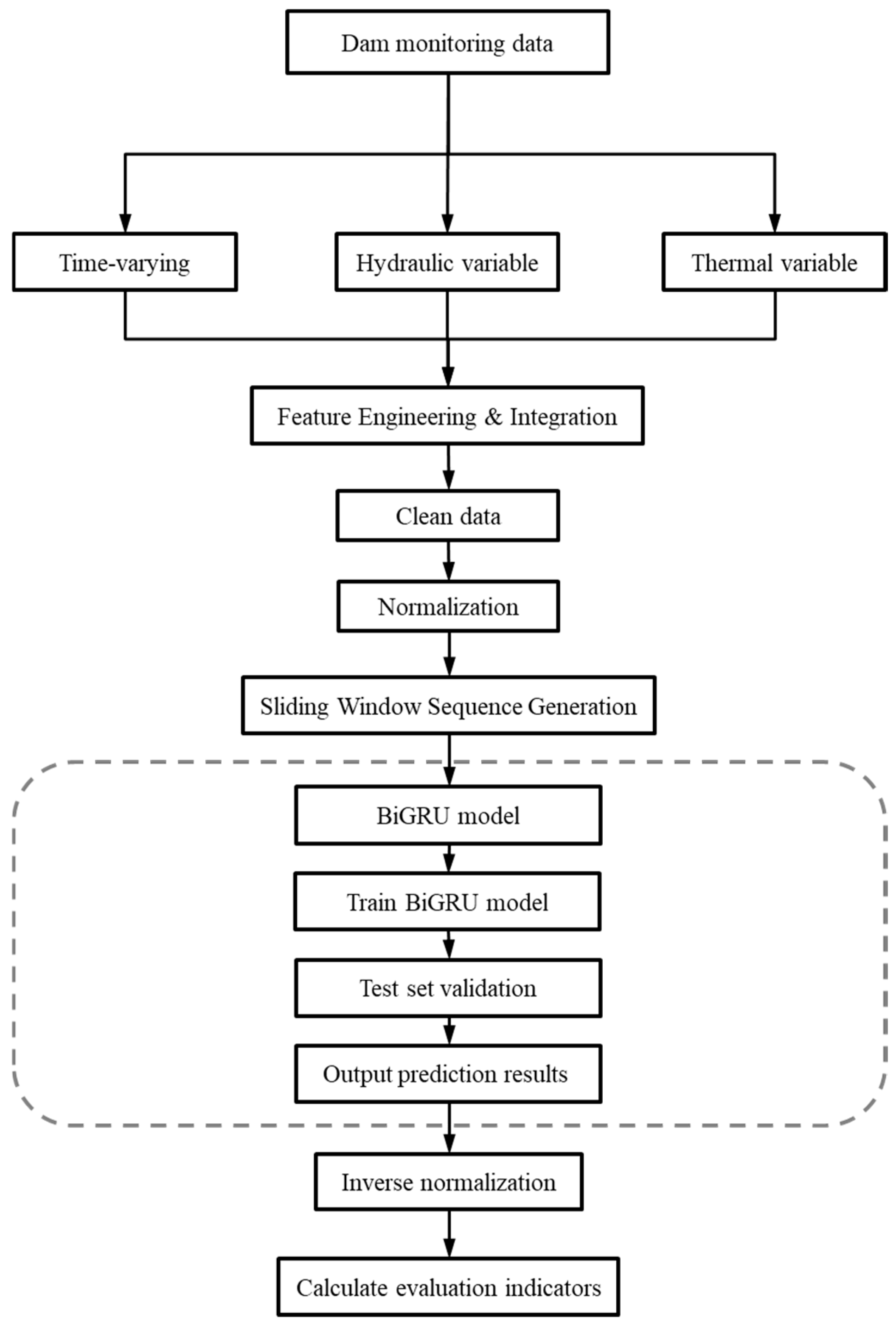
As illustrated in Figure 1, this framework is conceptually guided by the classical hydrostatic–seasonal–time (HTT) model’s principles and implemented using a powerful bidirectional gated recurrent unit (BiGRU) neural network. The implementation comprises three sequential phases: (1) Feature engineering guided by the HTT framework: Instead of performing a statistical decomposition, this phase focuses on selecting and engineering a comprehensive feature set. We utilize the raw monitoring variables that correspond to the HTT components (e.g., water levels for the hydrostatic effect, temperatures for the thermal effect). These are then enhanced with additional time-series features (e.g., lagged values and rolling statistics of the displacement) to holistically capture the time-dependent effects, such as material creep and seasonal patterns. (2) Sequence construction via sliding window: The resulting multi-feature time series is then partitioned using a sliding window technique. This creates discrete yet overlapping intervals, thereby capturing sequential dependencies and inherent time-lag characteristics intrinsic to dam deformation mechanisms; (3) Predictive modeling with a BiGRU: Finally, the preprocessed sequences are fed into the BiGRU architecture. 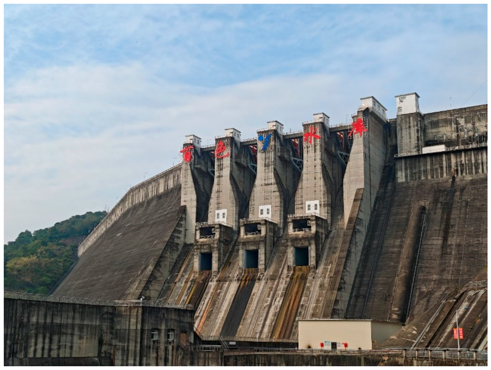The network leverages forward–backward propagation to model non-linear interactions between historical and future states, ultimately generating long-term deformation forecasts alongside corresponding statistical evaluation metrics (RMSE, MAE, R²). To ensure operational validity, the framework is rigorously validated through an engineering case study of a 130 m-high concrete gravity dam with over 18 years of operational history. Four strategically positioned monitoring points are utilized to evaluate spatiotemporal prediction accuracy across distinct dam zones.

2.1. Hydraulic–Thermal Transfer (HTT) Statistical Model

The Hydraulic Structure Temperature (HST) model utilizes harmonic functions to represent thermal variations yet fails to adequately explain thermally induced displacements arising from both short-term ambient temperature fluctuations and multi-year climatic variations. Conversely, the HTT model directly derives its thermal component from in situ temperature measurements, achieving a superior accuracy in modeling real-world dam monitoring data. The HTT framework decomposes concrete dam displacements (δ) into three constitutive terms: the static hydrostatic pressure component (δ_H), the thermal effects component (δ_T), and the time-dependent creep component (δ_θ), expressed as:

$$\delta ={\delta }_H+{\delta }_T+{\delta }_{\theta }$$

(1)

The hydrostatic component (δ_H) is governed by the reservoir elevation, expressed as:

$${\delta }_H={\displaystyle \sum _{i=1}^n{a}_i}{H}^i$$

(2)

where a_i are the regression coefficients; H denotes the reservoir elevation, with the exponent n = 3 for gravity dams and n = 4 for arch dams.

The thermal component δ_T characterizes thermally induced displacements from concrete and foundation temperature fluctuations, calculated using measured temperatures:

$${\delta }_T={\displaystyle \sum _{i=1}^m{b}_i}{T}_i$$

(3)

where b_i are the thermal regression coefficients, m indicates the number of temperature sensors, and T_i represents the measured temperature values.

The time-dependent component represents concrete creep deformation:

$${\delta }_{\theta }=c_1\theta +c_2\ln \theta$$

(4)

$$\theta =t/100$$

(5)

where c₁ and c₂ are the time-effect coefficients, and t denotes the cumulative operational days post-construction.

The aforementioned equations represent the classical statistical formulation of the HTT model, which provides a robust theoretical basis for understanding the primary factors of dam displacement. However, this traditional approach often assumes linear relationships and may struggle to capture the full spectrum of complex, non-linear dynamics inherent in dam behavior.

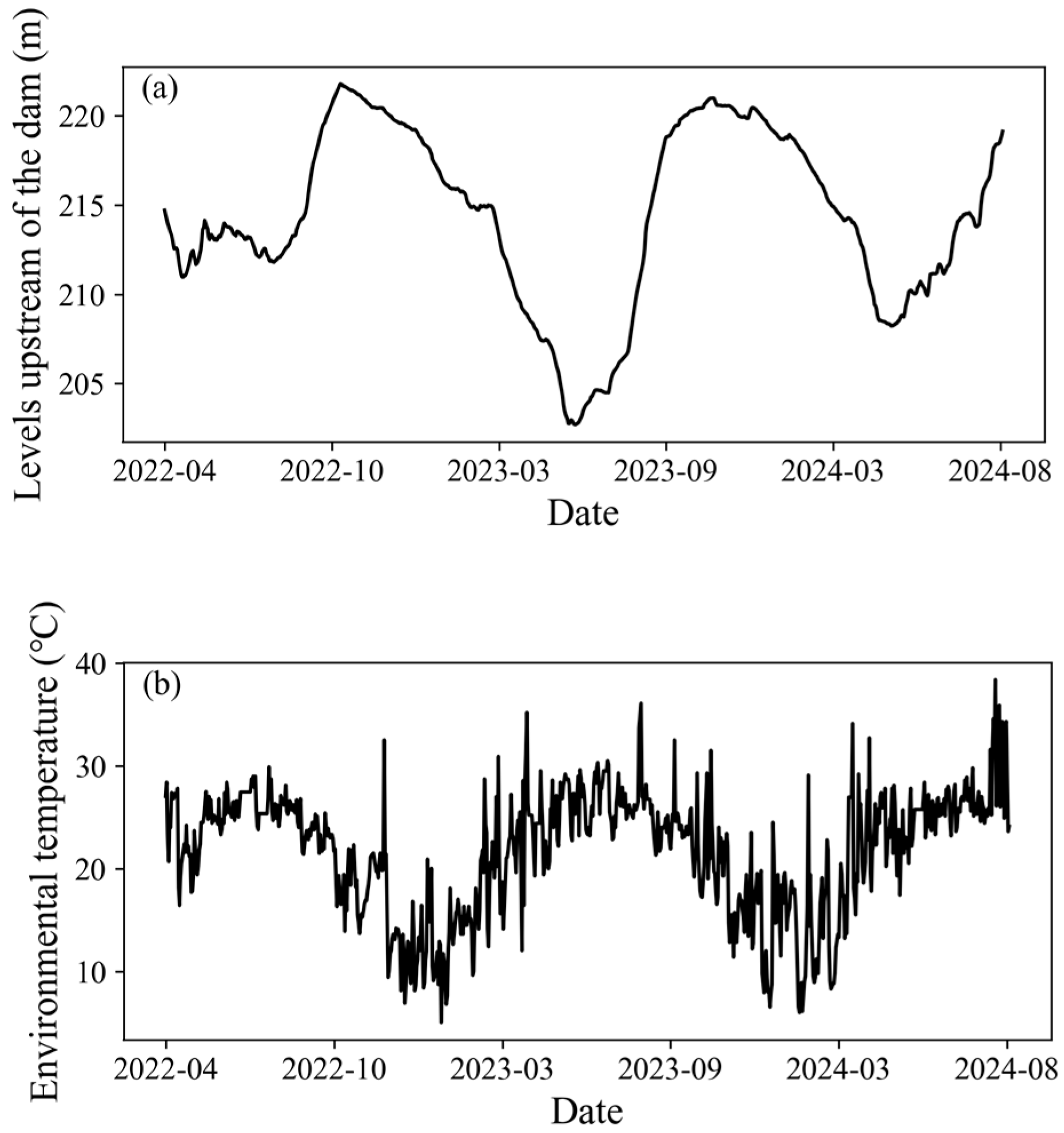
Therefore, in our proposed framework, we pivot from this statistical decomposition. Instead of using the calculated components (δ_H, δ_T, δ_θ) as inputs, we leverage the fundamental principles of the HTT model to guide our feature engineering. The raw physical variables that constitute these components (i.e., water levels, temperatures, and time-related markers) are fed directly into a deep learning network. This data-driven methodology allows the BiGRU model to learn the underlying non-linear relationships directly, offering the potential for a more accurate and comprehensive prediction.

2.2. BiGRU Model

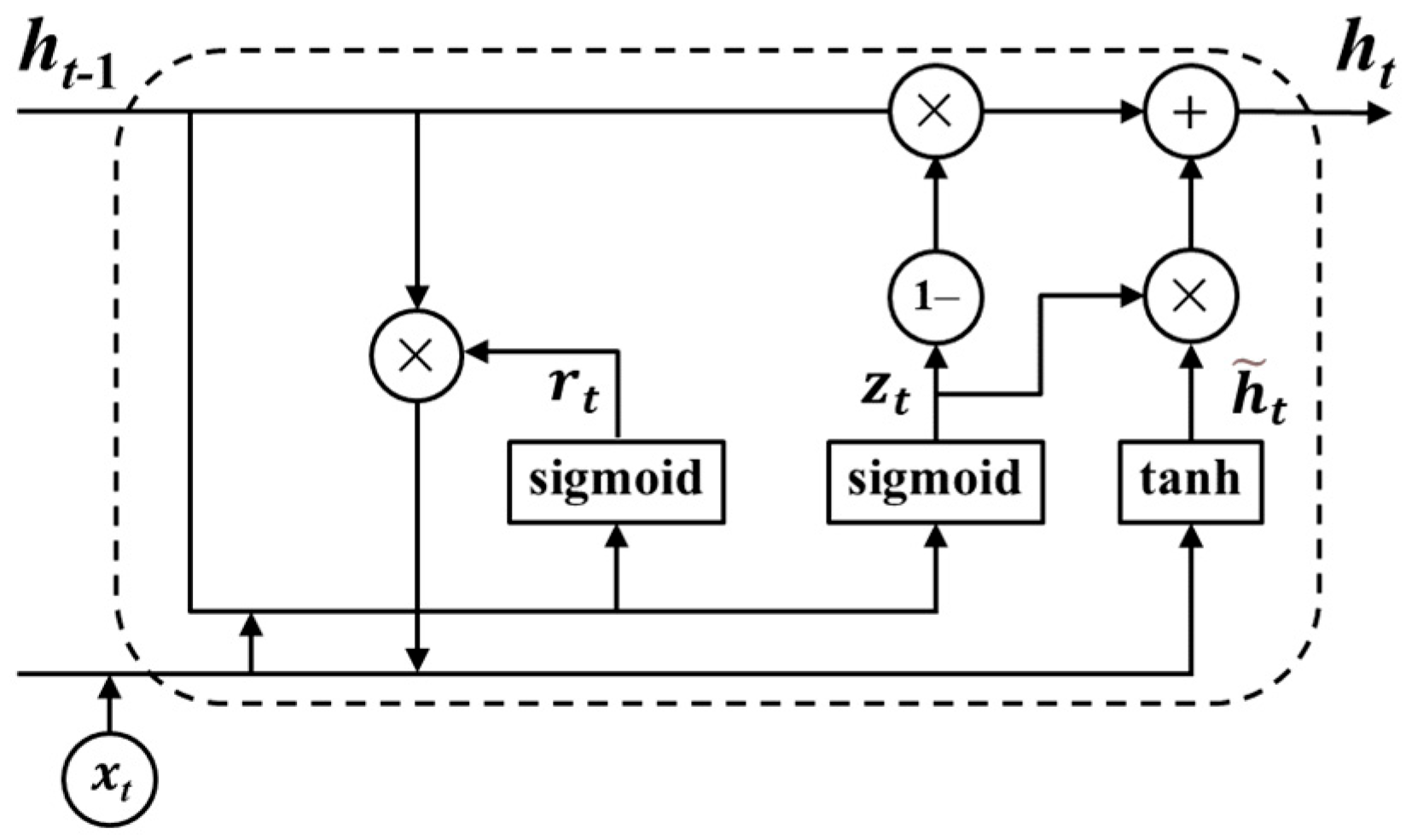
Traditional Recurrent Neural Networks (RNNs) are constrained by vanishing gradient and exploding gradient phenomena, which impair their performance on long-sequence modeling. The GRU addresses these limitations through gating mechanisms—a reset gate (r_t) for short-term pattern extraction and an update gate (z_t) for long-term state retention [23]. Figure 2 illustrates its computational graph at a single time step:

x_t denotes the input vector of the time point, z_t denotes the update gate, r_t denotes the reset gate, h_t−1 denotes the hidden state, $\tilde{h}$ denotes the candidate hidden state, and h_t denotes the updated hidden state. The sigmoid function (σ) generates gate activations (0–1), controlling information flow:

$$r_t=\sigma (W_r\cdot [h_{t-1},x_t])$$

(6)

$$z_t=\sigma (W_z\cdot [h_{t-1},x_t])$$

(7)

$${\tilde{h}}_t=\tanh (W_{\tilde{h}}\cdot [r_t\odot h_{t-1},x_t])$$

(8)

$$h_t=(1-z_t)\odot h_{t-1}+z_t\odot {\tilde{h}}_t$$

(9)

where $\odot$ denotes element-wise multiplication. The update gate interpolates between prior state retention (z_t → 0) and new state adoption (z_t → 1), while the reset gate r_t modulates historical information integration.

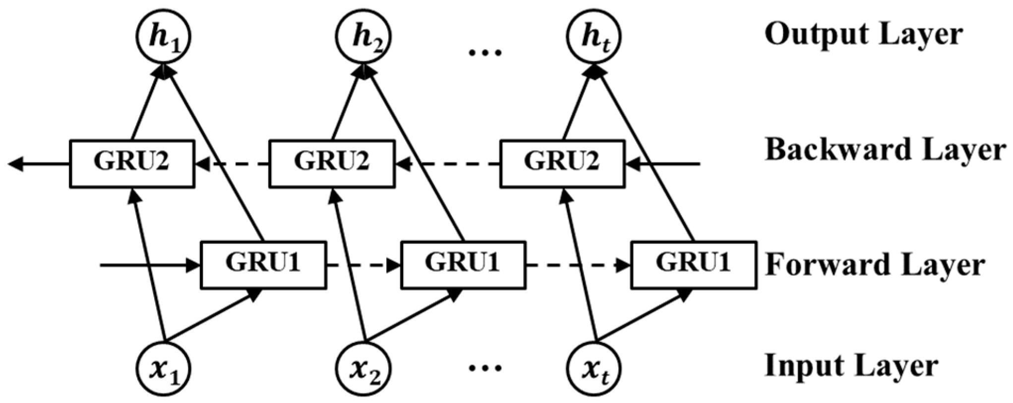
The BiGRU extends the GRU’s representational power through dual-directional sequence processing. By jointly analyzing forward (past-to-future) and reverse (future-to-past) contexts, the BiGRU captures comprehensive temporal patterns, demonstrating superior performance in sequential modeling tasks. As shown in Figure 3, the BiGRU framework integrates two GRU layers. The architecture implements bidirectional temporal processing through two complementary units: the forward GRU extracts features by propagating hidden states chronologically from timestep t = 1 to t = T, capturing historical dependencies, while the backward GRU operates inversely, propagating from t = T to t = 1 to model future-influenced patterns. Hidden state outputs from both directions are concatenated, enabling a synergistic integration of past and future contextual information for enhanced sequential representation learning.

At each time step t, the forward hidden state $h_t^{fw}$ and backward hidden state $h_t^{bw}$ are computed independently as follows:

$$h_t^{fw}=\mathrm{GRU}(x_t,h_{t-1}^{fw})$$

(10)

$$h_t^{bw}=\mathrm{GRU}(x_t,h_{t+1}^{bw})$$

(11)

The final output y_t concatenates both states as:

$$y_t=[h_t^{fw};h_t^{bw}]$$

(12)

This bidirectional architecture enables the synergistic learning of historical influences and future trends, providing a holistic representation of time-series dynamics.

2.3. Rolling Window Feature Engineering

To address delayed hydrological effects in dam monitoring, we employ rolling window aggregation to inject temporally shifted context into the HTT framework. W_τ = [t − τ, t − 1] defines a backward-looking window of days. The method computes six statistical descriptors over W_τ as:

$${\mathit{s}}_t={\left[\mu ,\tilde{x},\sigma ,max,min,IQR\right]}_{{\mathcal{W}}_{\tau }}$$

(13)

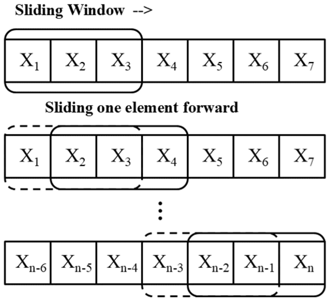
where μ denotes the mean, $\tilde{x}$ denotes the median, σ denotes the standard deviation, max denotes the max, min denotes the min, and IQR denotes the interquartile range. As diagrammed in Figure 4, for τ = 3, these features derive from the interval [t − 3, t − 1], creating a 72 h contextual prior. The engineered features s_t are concatenated with raw inputs x_t as:

$${\widehat{\mathit{x}}}_t={\mathit{x}}_t\oplus {\mathit{s}}_t$$

(14)

where $\oplus$ denotes the feature concatenation. The enriched input ${\widehat{\mathit{x}}}_t$ feeds into the BiGRU layer, enabling a simultaneous learning of instantaneous signals and historical trends. Explicit feature engineering enhances interpretability by quantifying how statistical properties of past observations influence current predictions.

3. Case Study

3.1. Project Description

This case study focuses on the main dam of the Baise Water Control Project in Guangxi, China. The front view of the dam is illustrated in Figure 5. The Baise Water Control Project began construction in 2001 and was completed in 2006.

Table 1. Information of Baise Water Control Project.

Items	Values
Drainage Area Proportion	47.57%
Average Annual Flow	263.0 m3/s
Annual Runoff	8.29 billion m3
Normal Pool Level (NPL)	228.0 m
Reservoir Area	135 km2
Backwater Length	108 km
Design Flood Level	229.66 m
Check Flood Level	231.27 m
Flood Control Restriction Level	214.0 m
Dead Water Level	203.0 m
Total Reservoir Capacity	5.66 billion m3
Flood Control Capacity	1.64 billion m3
Regulating Capacity	2.62 billion m3
Dead Storage Capacity	2.18 billion m3
Hydropower Station Capacity	540 MW
Navigation Structure Design	2 × 500-ton-class ships
Engineering Category	Class I engineering structure

presents the monitored hydraulic design parameters of the Baise Water Control Project.

The dam complex consists of the main dam, a hydropower station, two auxiliary dams, and the first phase of the navigation building, arranged in a decentralized layout. The main dam is a full-section roller-compacted concrete dam with a maximum height of 130 m, a crest length of 720 m, and 27 monoliths. The spillway section is 88 m long, and equipped with four overflow surface gates and three flood discharge mid-level outlets, with a maximum discharge capacity of 13,737 m³/s.

Based on the actual monitoring data and spatial distribution of the monitoring points, four representative monitoring points were selected from the distinct zones of the dam to serve as training samples. These points (TC3-1, TC3-11, TC3-12, and TC3-17) are vertical displacement sensors located at the dam crest. Their specific locations are shown in Figure 6 (schematic diagram of dam cross-section layout).

3.2. Data Collection and Preprocessing

The study analyzed daily monitoring data collected between April 2022 and August 2024. Figure 7 presents the temporal variations in the environmental parameters, including reservoir level and temperature. The reservoir level fluctuated seasonally, peaking at 223 m during flood seasons and reaching a minimum operational level of 202 m in dry periods. To mitigate flood risks associated with the summer monsoon rainfall, annual drawdown operations reduced the reservoir to its flood control level (202 m) from February to April. Post-monsoon replenishment restored the reservoir to its normal operating level (215 m) to support winter hydropower generation and irrigation demands.

Figure 8 details the vertical displacement patterns recorded at four crest monitoring points on the main dam. Globally, displacement data across the monitoring points display a seasonal trend: a downward trajectory from summer (June–August) to winter (December–February), followed by a gradual ascent to peak values in spring (March–May). Comparative analysis revealed a substantial heterogeneity in the initial displacements among the four monitoring points, with distinct variation ranges and amplitudes. Notably, discontinuous displacement patterns were identified in all monitoring datasets, attributable to the combined effects of natural factors (e.g., temperature fluctuations) and anthropogenic activities. These irregularities complicate the model’s capacity to discern dominant features within the high-dimensional data space.

To ensure optimal convergence and model robustness, a bifurcated data conditioning regimen was strategically implemented. The input features underwent Z-score standardization (Equation (15)), a process that normalizes each feature to a zero mean and unit variance. This standardization is critical for mitigating the influence of disparate feature scales and enhancing robustness to outliers, which are common in real-world environmental data. Concurrently, the target variable was subjected to Min–Max normalization (Equation (16)), a transformation that confines its values to the bounded [0, 1] interval. This latter procedure stabilizes the predictive target for the network’s output layer, thereby facilitating a more stable and efficient gradient descent during training. This dual-pronged strategy is predicated on the rationale that conditioning inputs and outputs differentially according to their roles maximizes the efficacy of the learning algorithm.

$$x_{\mathrm{standard}}={\displaystyle \frac{x-\mu }{\sigma }}$$

(15)

where x represents the original value of the feature, while μ and σ denote the mean and standard deviation of that feature, respectively.

$$x_{\mathrm{norm}}={\displaystyle \frac{x-\min (x)}{\max (x)-\min (x)}}$$

(16)

where x refers to the original data; x_norm refers to the normalized data.

3.3. Evaluation Metrics

Three evaluation metrics were employed to assess the predictive performance of the model: Root Mean Square Error (RMSE), Mean Absolute Error (MAE), and Coefficient of Determination (R²). The corresponding mathematical expressions are defined as:

$$RMSE=\sqrt{{\displaystyle \frac{1}{n}}{\displaystyle \sum _{i=1}^n{\left|y_i-{\widehat{y}}_i\right|}^2}}$$

(17)

$$MAE={\displaystyle \frac{1}{n}}{\displaystyle \sum _{i=1}^n|}{y}_i-{\widehat{y}}_i|$$

(18)

$$R^2=1-{\displaystyle \frac{{\displaystyle \sum _{i=1}^n{\left(y_i-{\widehat{y}}_i\right)}^2}}{{\displaystyle \sum _{i=1}^n{\left(y_i-\overline{y}\right)}^2}}}$$

(19)

where ${\hat{y}}_i$ denotes the predicted values, y_i represents the actual values, $\overline{y}$ is the mean of all samples, and n is the total number of samples.

3.4. Model Implementation and Hyperparameter Tuning

After defining the data, evaluation metrics, and the general BiGRU architecture, the next crucial phase is to implement the model and systematically optimize its parameters for the specific context of this case study. Generic model architecture rarely yields optimal results; therefore, a two-stage tuning process was employed to ensure the model’s configuration was best suited for the predictive task. First, we optimized the key feature engineering parameter—the rolling window size. Second, with the optimal features established, we proceeded to tune the internal hyperparameters of the BiGRU model itself. This data-driven approach ensures the model’s robustness and maximizes its predictive performance.

3.4.1. Optimization of Rolling Window Size

The construction of the time-series features using a rolling window is fundamental to providing the model with temporal context. The size of this window dictates a critical trade-off: a smaller window is more sensitive to recent fluctuations but can be susceptible to noise, while a larger window provides smoother features at the cost of increased lag.

To empirically determine the optimal window size, a comparative experiment was conducted. We evaluated a range of window sizes, including 2, 3, 4, 5, 7, and 10. For each size, the full data processing and model training pipeline was executed while holding all other model hyperparameters (e.g., neuron counts, learning rate) constant at a baseline value. The model’s performance was assessed using the RMSE, MAE, and R² metrics, as defined in Section 3.3.

The comprehensive results of this experiment are presented in

Table 2. Comparison of model performance for different rolling window sizes.

Window Size	Metrics	2	3	4	5	7	10
TC3-1	RMSE	1.51	1.44	1.62	1.59	1.61	1.58
	MAE	1.05	0.98	1.18	1.13	1.16	1.14
	R2	0.87	0.89	0.85	0.86	0.86	0.85
TC3-11	RMSE	2.09	1.54	2.16	2.07	4.21	3.21
	MAE	1.52	0.91	1.46	1.89	3.74	2.72
	R2	0.85	0.93	0.84	0.85	0.45	0.67
TC3-12	RMSE	2.21	2.06	2.16	2.16	2.94	2.59
	MAE	1.72	1.43	1.61	1.52	2.29	1.84
	R2	0.92	0.94	0.92	0.93	0.84	0.86
TC3-17	RMSE	1.84	1.76	1.81	1.84	1.98	1.97
	MAE	1.44	1.39	1.42	1.54	1.64	1.57
	R2	0.77	0.81	0.79	0.72	0.69	0.71

. The analysis indicates that a window size of three consistently yielded a superior or highly competitive performance across the majority of the datasets. It achieved a robust balance between capturing meaningful short-term dynamics and maintaining feature stability. Therefore, a rolling window size of three was selected for all feature engineering in the subsequent stages of this study.

3.4.2. BiGRU Model Hyperparameter Optimization

With the input features defined by the optimal rolling window size, the next step was to optimize the BiGRU model’s internal architecture. This process is essential for ensuring the model’s robustness and tailoring its complexity to the specific dataset, thereby preventing over- or under-fitting.

For this task, we employed the Keras Tuner library, a dedicated tool for hyperparameter optimization. We utilized the Hyperband algorithm, an efficient search strategy, to find the best combination of hyperparameters by minimizing the validation loss (val_loss). The search space was defined to include the model’s most critical parameters: Units in the first BiGRU layer—an integer value between 32 and 256 (step size: 32); units in the second BiGRU layer—an integer value between 16 and 128 (step size: 16); dropout rates—a floating-point value between 0.2 and 0.5 (step size: 0.1); and learning rate—a selection from the set {0.01, 0.001, 0.0001}.

The optimization process automatically trained and evaluated numerous model configurations. The best-performing set of hyperparameters identified through this search is detailed in

Table 3. Optimal hyperparameters for the BiGRU model.

Hyperparameter	Optimal Value
Units (Layer 1)	160
Dropout Rate (Layer 1)	0.3
Units (Layer 2)	80
Dropout Rate (Layer 2)	0.2
Learning Rate	0.001

. All final model training, evaluation, and analysis presented in Section 4 were conducted using this optimized hyperparameter configuration.

4. Results

4.1. Experimental Setup

To ensure the transparency and reproducibility of our research, it is essential to document the precise configuration of the experimental environment. Accordingly, all pertinent details regarding the hardware platform, software dependencies, and the final model hyperparameters employed in this study are systematically summarized in

Table 4. Experimental environment and model hyperparameters.

Category	Item	Specification
Hardware	CPU	Intel(R) Core (TM) i7-10700 CPU @ 2.90 GHz
	GPU	NVIDIA GeForce GT 730
	Memory (RAM)	15.74 GB
	Operating System	Windows 10
Software	Python	3.11.4
	TensorFlow	2.18.0
	Scikit-learn	1.6.1
	Pandas	2.2.3
	Numpy	2.0.2
	Kerastuner	1.0.5
Hyperparameters	Model Architecture	2-Layer Bidirectional GRU
	Units (Layer 1)	160
	Dropout Rate (Layer 1)	0.3
	Units (Layer 2)	80
	Dropout Rate (Layer 2)	0.2
	Optimizer	Adam
	Learning Rate	0.001
	Loss Function	Mean Squared Error (MSE)
	Batch Size	32
	Epochs	Up to 500, with Early Stopping (Patience = 20)

. This information includes the specifications of the computing hardware, the versions of key libraries, and the optimal parameter values determined through the tuning processes described in the preceding sections.

4.2. Model Training and Convergence Analysis

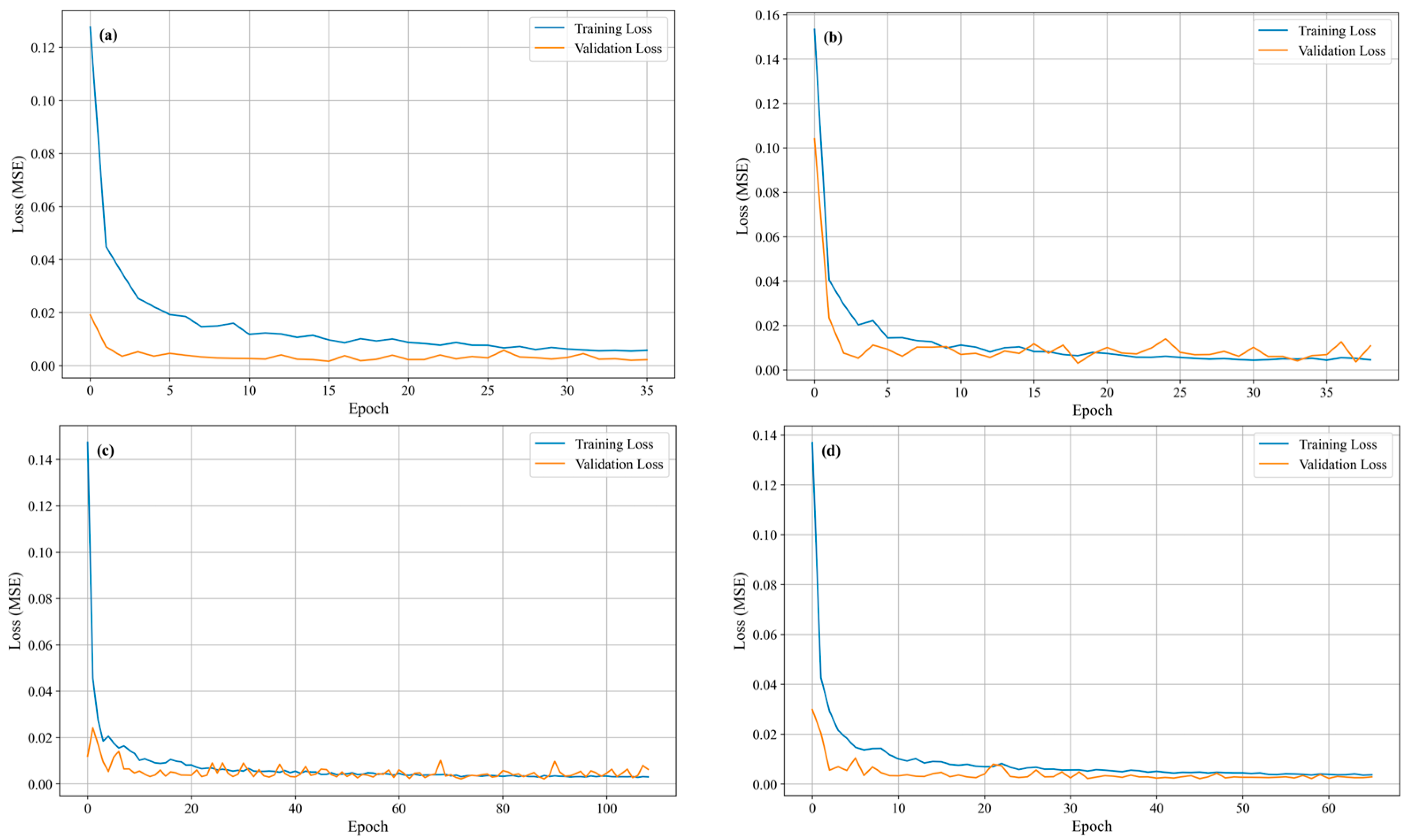
To analyze the convergence and stability of the model during the training phase, the learning curves for the optimized BiGRU model at each of the four monitoring points are presented in Figure 9. A consistent and desirable training pattern is observed across all four subplots (a–d).

In each case, both the training loss and validation loss decrease sharply during the initial epoch, indicating that the model learns the primary data patterns rapidly. Subsequently, the curves flatten and converge to a stable, low value. Crucially, the validation loss curve closely tracks the training loss curve throughout the entire process, without any significant divergence. This proximity between the two curves provides strong evidence that the models achieved effective generalization without overfitting the training data. Furthermore, the varying number of total epochs in each subplot demonstrates the effective functioning of the Early Stopping mechanism, which terminated the training process optimally for each case once the validation loss ceased to improve.

4.3. Comparative Analysis of Model Performance

To benchmark the baseline model performance, four time-series forecasting architectures—LSTM, BiLSTM, GRU, and BiGRU—were trained on raw measured displacement data using a three-step sliding window with default hyperparameters. The model’s generalization capability was evaluated through long-term prediction accuracy and standard evaluation metrics. As the dam’s service duration extends, operational monitoring datasets exhibit a progressive temporal expansion.

The quantitative evaluation of the proposed method and baseline models for long-term dam displacement prediction is summarized in

Table 5. Predictive performance comparison of BiGRU against three canonical time-series deep learning models.

Monitoring Point	Metrics	LSTM	BiLSTM	GRU	BiGRU
TC3-1	RMSE	2.21	2.31	1.65	1.44
	MAE	1.68	1.67	1.17	0.98
	R2	0.73	0.70	0.85	0.89
TC3-11	RMSE	2.31	3.97	3.14	1.54
	MAE	1.69	3.18	2.69	0.91
	R2	0.84	0.48	0.70	0.93
TC3-12	RMSE	3.06	3.99	2.07	2.06
	MAE	2.56	3.28	1.55	1.43
	R2	0.86	0.74	0.93	0.94
TC3-17	RMSE	2.21	2.16	1.65	1.76
	MAE	1.83	1.71	1.30	1.39
	R2	0.71	0.69	0.84	0.81

. The BiGRU algorithm consistently outperformed other architectures across all four monitoring points, demonstrating an enhanced generalization capacity and robust stability. This superiority stems from its dual-directional memory propagation mechanism, which adaptively weights historical context and future-inferred patterns—a critical advantage when processing sparse or asynchronous monitoring data. When using the correlation coefficients as the evaluation metric, the BiGRU exhibited statistically significant improvements over LSTM, BiLSTM, and GRU, with performance gains closely aligned with the complexity of each baseline’s temporal dependency modeling capability. These results demonstrate that the BiGRU is capable of extracting meaningful patterns from four distinct and weakly correlated datasets, validating its effectiveness in disentangling heterogeneous spatiotemporal couplings within dam systems.

4.4. Visual Analysis of Prediction Results

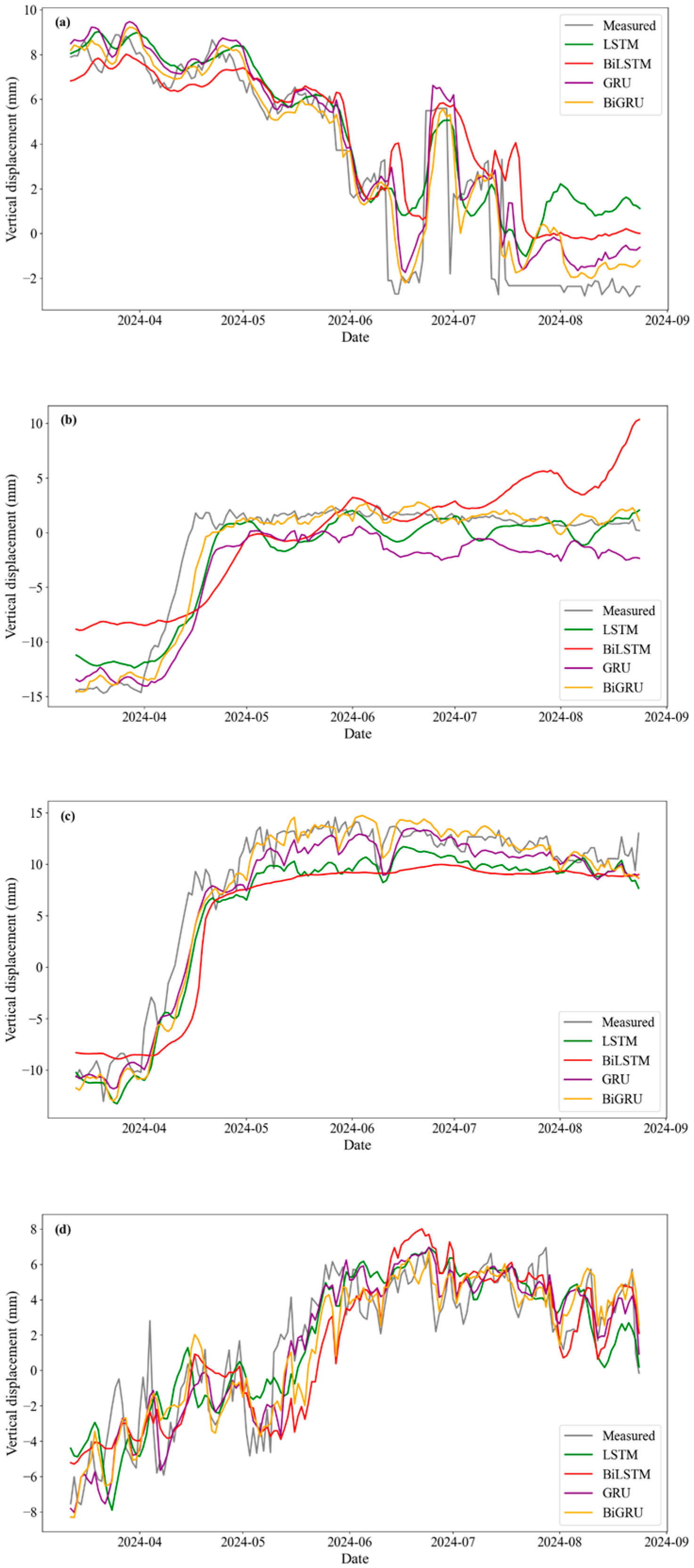
Figure 10 provides a comparative visualization of the long-term prediction performance between the proposed method and baseline models, validated against monitoring data collected from April to August 2024. The BiGRU model shows the strongest agreement with observational trends during the local temporal interval (April–July), achieving the lowest overall prediction error among all models. Its trajectory closely follows the phase-shifted deformation pulses induced by delayed reservoir seepage pressures—an effect that unidirectional models fail to capture effectively. All methods exhibit residual inaccuracies during the terminal prediction phase (August 2024), with errors systematically increasing compared with earlier stages. This divergence becomes more pronounced near hydrological transition periods, where conventional models struggle to reconcile rapid water level fluctuations with slow-moving creep deformations. The consistent performance degradation across models highlights the inherent challenges in maintaining predictive stability over extended horizons, underscoring the necessity of memory-gated architectures for effective error attenuation.

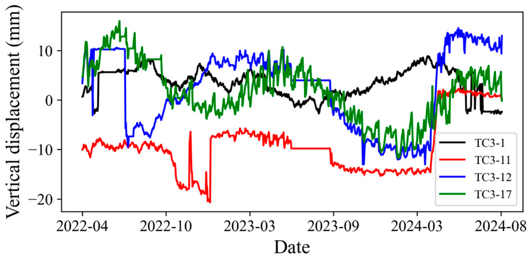
The observed difference in the magnitude of displacement fluctuations between the monitoring points can be attributed to the distinct structural characteristics and boundary conditions at their respective locations on the dam.

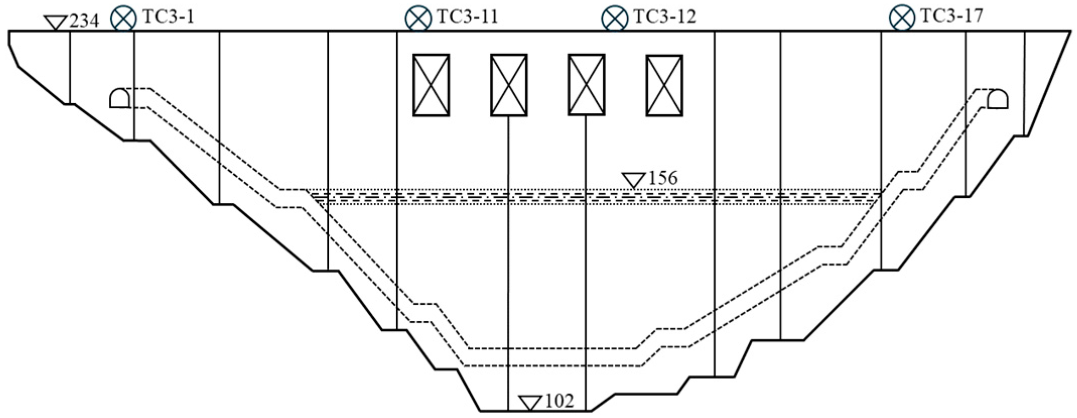
Points TC3-1 and TC3-17 are situated at the dam abutments, where the concrete structure is anchored into the bedrock of the valley sides. As shown in the profile diagram, these sections are thinner and have a smaller volume compared to the central monoliths. This lower thermal mass makes them more susceptible to ambient temperature variations, leading to more pronounced and frequent cycles of expansion and contraction. This heightened sensitivity to thermal effects is the primary reason for the larger displacement fluctuations observed at the dam’s flanks.

In contrast, points TC3-11 and TC3-12 are located on the crest of the massive central dam monoliths, directly above the powerhouse and spillway block. Due to their enormous volume, these sections possess significant thermal inertia, meaning their temperature changes much more slowly and is less influenced by short-term air temperature swings. Consequently, their displacement behavior is more stable and is predominantly governed by the more slowly varying hydrostatic pressure from the reservoir. Therefore, while their absolute displacement may be substantial, the fluctuations around their mean positions are less significant than those at the abutments.

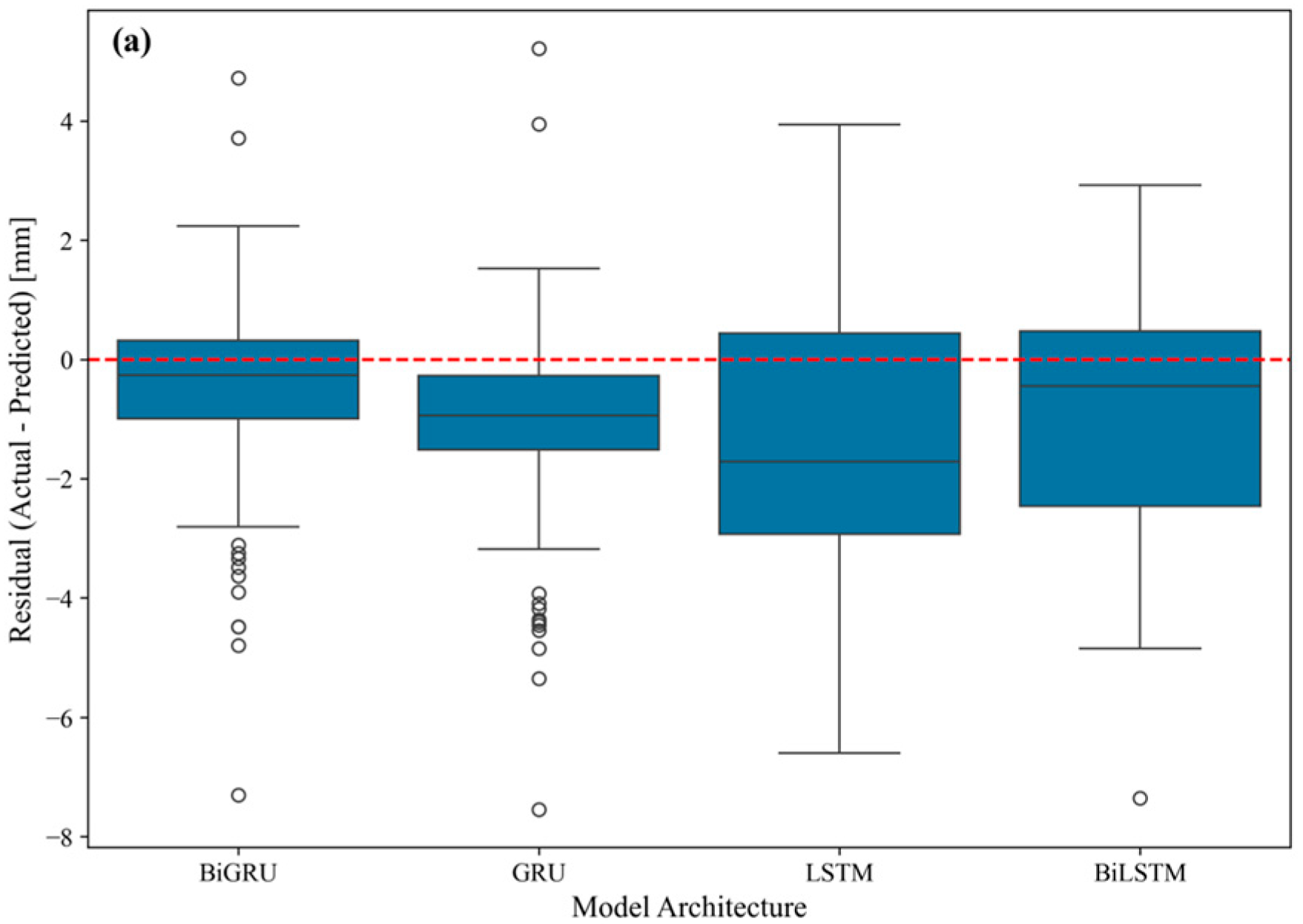
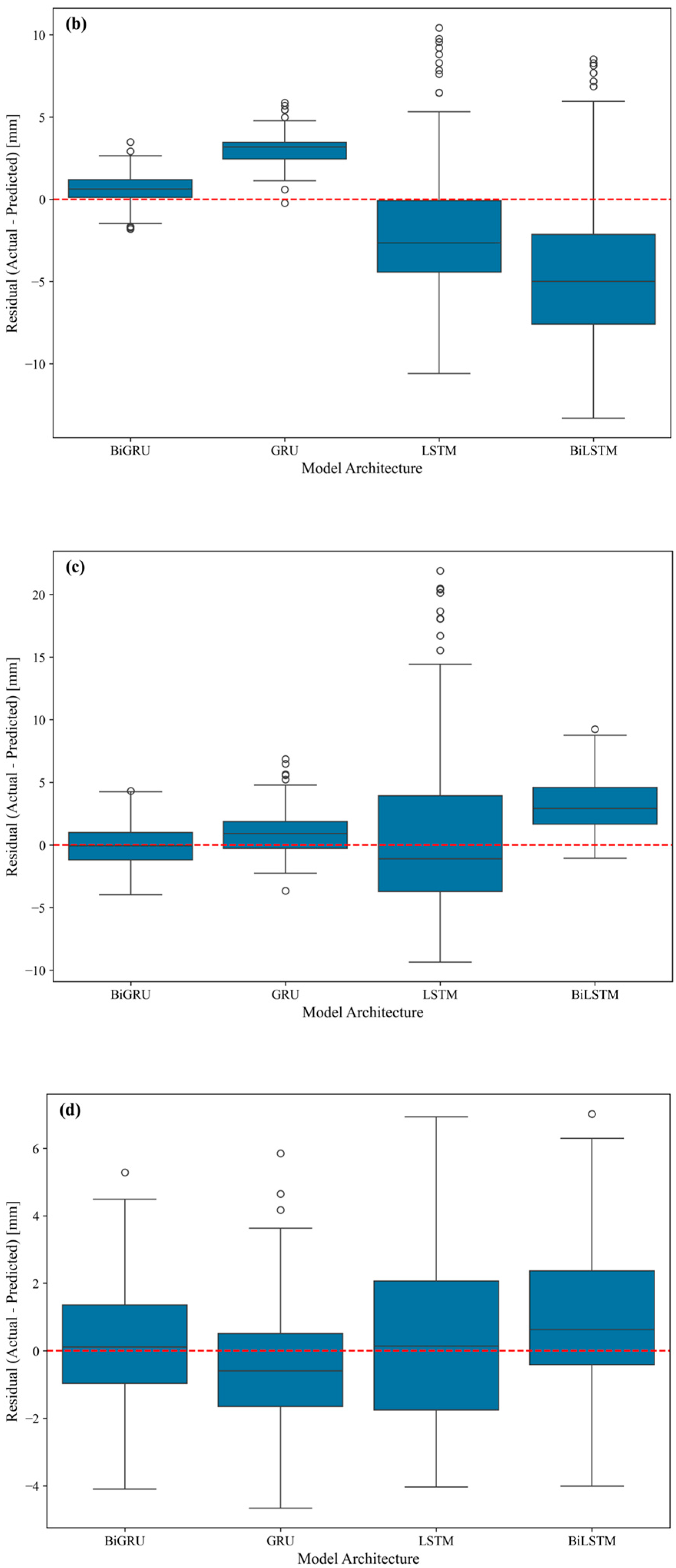
The proposed BiGRU-based predictive framework demonstrates an exceptional generalization capability and interpretability, achieving a superior average performance across all four monitoring points with an R² of 0.89, an MAE of 1.17 mm, and an RMSE of 1.70 mm. This performance represents a significant leap over conventional architectures; for instance, compared to the standard GRU model—the strongest of the benchmarks—our proposed model delivered a 20.2% reduction in RMSE and a 30.4% reduction in MAE. This quantitative superiority is visually substantiated by the analysis presented in Figure 11, where the BiGRU model’s residual box plots consistently exhibit a more compact and zero-centered error distribution. While the standard GRU showed competitive performance at a single point, the BiGRU model’s consistent high accuracy across all locations underscores its superior stability and robustness. These findings indicate that the synergistic integration of the bidirectional architecture and sliding window optimization enables the model to effectively extract latent spatiotemporal patterns, making it a promising solution for long-term displacement forecasting in concrete gravity dams.

5. Conclusions

In this study, we developed and validated an enhanced predictive framework for dam displacement by integrating a Bidirectional GRU (BiGRU) with optimized time-series feature engineering. The primary contributions and findings of this work are summarized as follows:

(1)

Novel hysteresis-aware framework: A predictive model was established that explicitly accounts for the hydraulic hysteresis effects in dam behavior. This was achieved by synergizing a BiGRU architecture, which captures the temporal dependencies from both past and future contexts, with a sliding window mechanism for dynamic feature extraction.

(2)

Systematic model optimization: The model’s robustness and configuration were not arbitrary but were determined through a rigorous, two-stage optimization process. A preliminary comparative experiment identified the optimal rolling window size (τ = 3) for feature engineering, followed by a systematic hyperparameter tuning process to ascertain the ideal network architecture, learning rate, and regularization parameters.

(3)

Superior quantitative performance: The optimized BiGRU model demonstrated superior predictive accuracy and generalization ability. Across all four monitoring points, it achieved an average R² of 0.89 and an RMSE of 1.70 mm. This represents a substantial improvement over the strongest benchmark model (standard GRU), with a 20.2% reduction in RMSE and a 30.4% reduction in MAE, providing concrete evidence of the framework’s value.

(4)

Enhanced temporal feature representation: The success of the model is attributed to the BiGRU’s dual-path processing (forward and backward), which distills a more comprehensive feature representation from complex multivariate time-series data compared to unidirectional models. This establishes a new paradigm for enhancing dam safety assessments through bidirectional temporal learning.

Despite the model’s strong performance, certain limitations highlight avenues for future research. First, the framework’s sensitivity to displacement anomalies induced by operational fluctuations or sensor drifts warrants the development of integrated data-cleaning and anomaly detection protocols. Second, as a dam deforms as an integrated system, future work should prioritize multi-point data fusion strategies. Investigating cross-correlation analysis and employing advanced methodologies, like graph neural networks, could better quantify the spatiotemporal interdependencies among monitoring points, which is essential for modeling the holistic behavior of the entire structure. Finally, the validation in this study was limited to monitoring points on the dam crest due to limited data availability; future work should aim to verify the model’s performance across the entire dam profile by incorporating data from its middle and base sections. Successfully addressing these limitations will lead to more robust predictive systems, providing operators with critical tools for proactive maintenance and asset management, and thereby ensuring the long-term sustainability and resilience of vital water infrastructure.