Abstract
With the deep integration of electricity and carbon trading markets, distribution networks are facing growing operational stress and a shortage of flexible resources under high penetration of renewable energy. This paper proposes a three-layer coordinated planning model for Source–Grid–Load–Storage (SGLS) systems, considering electricity–carbon coupling and flexibility supply–demand balance. The model incorporates a dynamic pricing mechanism that links carbon pricing and time-of-use electricity tariffs, and integrates multi-source flexible resources—such as wind, photovoltaic (PV), conventional generators, energy storage systems (ESS), and controllable loads—to quantify the system’s flexibility capacity. A hierarchical structure encompassing “decision–planning–operation” is designed to achieve coordinated optimization of resource allocation, cost minimization, and operational efficiency. To improve the model’s computational efficiency and convergence performance, an improved adaptive particle swarm optimization (IAPSO) algorithm is developed which integrates dynamic inertia weight adjustment, adaptive acceleration factors, and Gaussian mutation. Simulation studies conducted on the IEEE 33-bus distribution system demonstrate that the proposed model outperforms conventional approaches in terms of operational economy, carbon emission reduction, system flexibility, and renewable energy accommodation. The approach provides effective support for the coordinated deployment of diverse resources in next-generation power systems.
1. Introduction
With the deepening integration of electricity and carbon trading markets, power system planning is confronted with increasingly complex constraints and challenges. The rapid growth of renewable energy penetration has exacerbated system volatility and uncertainty, leading to severe wind and solar curtailment as well as insufficient flexibility. These issues highlight the urgent need for advanced planning methodologies capable of simultaneously ensuring economic efficiency, achieving low-carbon objectives, and maintaining operational security. The early studies on source-grid-load (SGL) coordinated planning primarily focused on the coordinated operation of generation, the grid, and the load, as well as uncertainty modeling on the supply side [1]. However, they paid insufficient attention to energy storage resources, which have been widely deployed in recent years to enhance systems’ flexibility [2,3]. In response, integrated planning approaches that consider SGLS have gradually emerged. These methods partially incorporate uncertainties on both the supply and demand sides, along with low-carbon development strategies. Nevertheless, most existing research has yet to thoroughly explore the mechanisms of interaction between electricity and carbon markets—referred to as electricity–carbon coupling—nor systematically analyze the impact of achieving a supply–demand balance in flexibility under such a coupling framework on the overall coordinated planning of a SGLS system. Therefore, developing a coordinated SGLS planning method that accounts for both electricity–carbon coupling and system flexibility holds significant theoretical and practical importance.
As a critical terminal component of power systems, the distribution network is characterized by a complex topology, a large scale, and diverse configurations. With the large-scale integration of distributed energy resources (DERs), traditional distribution network structures are increasingly inadequate in managing the power balancing challenges that arise from the combined effects of generation-side intermittency and load-side uncertainty [4]. Consequently, the planning of modern distribution networks is evolving into a multi-dimensional, complex optimization problem, featuring uncertainty, multi-objectivity, nonlinearity, dynamic behavior, and discrete decision variables [5]. According to [6], the widespread deployment of distributed energy and power electronic devices has significantly amplified system uncertainty, thereby increasing the complexity of planning problems. To address these challenges, a meshed distribution network planning approach has been proposed. This method divides the original system into multiple supply zones for partitioned optimization, effectively reducing the modeling dimensionality and simplifying the planning process [7].
In the field of SGLS coordinated planning, carbon trading mechanisms have been widely adopted to promote carbon emission reduction and optimize power generation structures. References [8,9] incorporate carbon trading constraints into generation-side capacity planning to limit the output of high-emission units. Reference [10] introduces a tiered carbon pricing mechanism in the dispatch of integrated energy systems, significantly enhancing the effectiveness of emission constraints. In [11,12], carbon pricing is embedded in system planning models to prioritize the siting of low-carbon technologies, which thereby improves the utilization of renewable energy sources. On the other hand, reference [13] employs a leader–follower game-theoretic approach to engage both supply and demand sides in demand response programs, achieving both economic efficiency and system load relief through peak shaving and valley filling. Reference [14] proposes a demand response potential forecasting method based on the electricity–carbon coupling incentive effect, which effectively improves the controllability and economic benefits of the demand response. Reference [15] introduces an integrated electricity–carbon trading linkage mechanism for the demand side, achieving the dual goals of carbon emission reduction and cost optimization through the joint optimization of electricity and carbon markets. In addition, references [16,17] present a weather-aware electricity price interval forecasting method and a large language model-based approach for assisting in bidding behavior and market sentiment analysis, providing new techniques for the joint forecasting of electricity and carbon prices. Across these studies, carbon trading mechanisms control emissions by adjusting carbon prices, while a price-based demand response achieves load shifting through electricity price signals. Both are fundamentally driven by market signals, which indicates an inherent correlation between electricity and carbon prices. However, most of the existing literature still treats the carbon trading mechanism as an independent factor, without thoroughly examining the potential impact of electricity–carbon coupling on integrated system planning.
However, the integration of electricity–carbon coupling mechanisms not only affects generation dispatch and investment but also exacerbates the need for system flexibility. As carbon pricing incentivizes higher renewable energy penetration, the variability and uncertainty of renewable resources increase, leading to significant flexibility challenges. Therefore, it is essential to integrate a flexibility supply–demand balancing framework into electricity–carbon coupled planning to ensure the secure and economic operation of the distribution network. Ensuring a balance between the supply and demand of flexibility has emerged as a core challenge for the sustainable operation of power systems [18,19]. A variety of flexibility-oriented planning approaches have been proposed in the literature. For instance, reference [20] presents a generation expansion model that incorporates flexibility balancing, which significantly enhances the system’s ability to accommodate the uncertainties of wind and solar power. Reference [21] highlights that neglecting flexibility considerations in planning may result in an inadequate system regulation capacity and even trigger operational risks. To address this, reference [22] develops a probabilistic flexibility margin model to quantify systems’ regulation capability, which is further extended into a bi-level optimization framework with upper–lower layer interactions [23,24]. In addition, some studies introduce flexibility metrics into SGLS coordinated planning models to achieve coordinated regulation of various resources [25] or to evaluate the flexibility supply capability in the contexts of thermal power retrofitting [26] and transmission network expansion [27]. Overall, the current research on system flexibility remains largely focused on the optimal configuration of supply-side resources, with limited attention being paid to demand-side flexibility resources—such as shiftable and interruptible loads—in terms of modeling and dispatch potential. Moreover, few studies incorporate these demand-side resources into a comprehensive flexibility supply–demand balancing framework under electricity–carbon coupling mechanisms. Investigating the influence of electricity–carbon market interactions on system flexibility regulation and developing a joint flexibility balancing model that involves both the demand and supply sides still present significant research opportunities.
In summary, most current approaches only focus on electricity pricing or carbon pricing separately, without fully revealing their intrinsic coupling relationship. Meanwhile, although some works have introduced flexibility-oriented planning concepts, they often neglect demand-side flexibility resources or lack a systematic framework for achieving flexibility supply–demand balance. Moreover, none of the existing studies simultaneously consider the combined effects of electricity–carbon coupling and flexibility supply–demand balance. In addition, conventional optimization algorithms, such as standard PSO or GA, suffer from slow convergence and a tendency to fall into local optima.
To overcome these limitations, this paper proposes a three-layer coordinated planning model that integrates electricity–carbon coupling and a flexibility supply–demand balance, while also introducing the IAPSO algorithm to enhance both the solution quality and computational efficiency. The main innovations and contributions of this paper are as follows:
- (1)
- Three-layer planning model development: a “decision–planning–operation” three-layer coordinated planning model is proposed, which incorporates electricity–carbon coupling and a flexibility supply–demand balance into a unified framework for source–grid–load–storage planning in distribution networks;
- (2)
- Electricity–carbon pricing mechanism: a dynamic electricity–carbon coupled pricing model is established to effectively guide resource allocation and investment decisions;
- (3)
- Flexibility supply–demand modeling: a comprehensive flexibility quantification approach is proposed that integrates both supply-side and demand-side flexibility resources for coordinated system operation;
- (4)
- Algorithmic improvement: an improved adaptive PSO algorithm is designed to accelerate convergence and enhance the global search capability for solving large-scale planning problems.
The remainder of this paper is organized as follows: Section 2 introduces the electricity–carbon coupled pricing model, Section 3 presents the flexibility supply–demand quantification model, Section 4 describes the three-layer coordinated planning model, Section 5 explains the IAPSO algorithm and solution methodology, Section 6 provides simulation results and discussions, and Section 7 concludes this paper.
2. Construction of the Electricity–Carbon Coupled Pricing Model
The interaction between the electricity market and the carbon trading market is fundamentally driven by electricity prices and carbon trading prices, as illustrated in Figure 1. When electricity demand rises, electricity prices increase, boosting the profit margins of both conventional and renewable generators. However, conventional units—such as coal-fired plants—must purchase carbon allowances proportional to their generation, which drives up carbon demand and carbon prices. As carbon prices climb, the profitability of conventional generators declines due to the additional carbon cost, which discourages capacity expansion and reduces their output, and thereby alleviates carbon demand. In contrast, renewable generators—unaffected by carbon costs—benefit from higher electricity prices and expand their capacity more rapidly. As the share of renewables in the generation mix grows, their zero-marginal-cost output exerts downward pressure on electricity prices. Meanwhile, the displacement of carbon-intensive conventional units by renewables reduces the overall carbon demand, which in turn suppresses carbon prices. Over time, these interactions lead the system to a dynamic equilibrium between electricity and carbon markets.
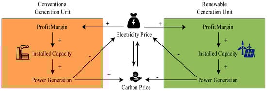
Figure 1.
Electricity–carbon coupled market.
Time-of-use (TOU) electricity prices are set by the upstream grid operator, while the dynamic carbon price is derived from the day-ahead carbon trading costs in the electricity–carbon coupled market. The dynamic carbon price is determined jointly by the benchmark carbon price and the known carbon emission factor. Therefore, accurately calculating the average carbon price for the distribution network is a key aspect in constructing the electricity–carbon coupled pricing model.
2.1. Carbon Trading Pricing Model
The total amount of carbon emissions traded on the previous day is calculated as shown in Equation (1).
where denotes the total carbon emissions traded on the previous day; is the baseline carbon emission rate of coal-fired units; represents the output of coal-fired units at time ; is the duration of each time interval; stands for the baseline carbon allowance for coal-fired units; and is the total number of time intervals.
According to carbon market regulations, a tiered carbon price is used to calculate the carbon emission cost. The tiered carbon price and the carbon emission cost are calculated as shown in Equations (2) and (3), respectively.
where is the initial carbon market trading price; is the carbon price growth rate; represents the system carbon allowance; is the length of the carbon emission interval (kg); is the number of emission intervals involved; the range from to is divided into the initial interval and the excess interval ; denotes the length of the carbon emission interval. The given segment denotes the length of the corresponding carbon emission interval. Positive carbon price intervals indicate that the system’s emissions exceed the allowance, which requires the purchase of carbon credits; negative intervals correspond to emissions below the allowance, which allows for the sale of surplus carbon credits for revenue.
The average carbon price is calculated based on the averaging principle, as shown in Equation (4).
The time-of-use carbon price over one day is given by Equation (5):
where , is the total number of time intervals in a day; is the dynamic carbon price at time ; is the carbon emission factor adjustment coefficient; denotes the carbon emission factor at time ; is the threshold value of the carbon emission factor; is the time-of-use electricity price coefficient; and and are the dynamic carbon pricing coefficients.
2.2. Tiered Electricity Pricing Model Under the Electricity–Carbon Coupled Market
Carbon trading prices and electricity prices serve as the primary interactive carriers in the electricity–carbon coupled market. By considering the dynamic interplay between the two, the market interaction can be expressed as follows:
where and represent the baseline time-of-use electricity price and baseline carbon trading price in the absence of electricity–carbon market coupling; and represent the time-of-use electricity price and carbon trading price under the coupled market; coefficients , , and denote the growth rate of the carbon allowance purchase cost, the electricity price reduction coefficient, and the electricity price growth coefficient, respectively, in the uncoupled market; coefficients , , and denote the corresponding parameters under the electricity–carbon coupled market.
This formulation establishes both the carbon trading pricing model and the tiered electricity pricing model under the electricity–carbon coupled market.
3. Flexibility Supply–Demand Quantification Model for Distribution Networks
The large-scale integration of wind and photovoltaic power, as the main forms of renewable energy, introduces significant variability and uncertainty, which increases the peak–valley gap of the net load. This, in turn, elevates the system’s flexibility demand. Therefore, it is essential to analyze the flexibility of the supply and demand capabilities of the system and to develop a flexibility balancing model that ensures the dynamic equilibrium of the flexibility of the supply and demand within the power system.
3.1. Flexibility Resource Modeling
(1) Conventional Units
The use of conventional units in power systems—primarily coal-fired power plants and gas turbines—offers advantages such as flexible siting, short construction periods, and the maturity of the associated technologies. However, due to limitations imposed by dispatch instructions, conventional units exhibit low ramp rates and limited flexibility in regulation [28]. The flexibility supplied by conventional units is expressed in Equation (7):
where and represent the upward and downward flexibility of conventional unit during time period
; , , and denote the maximum output, minimum output, and real-time output of conventional unit at time , respectively; and are the upward and downward ramp rates of unit ; and is the regulation time interval.
(2) Energy Storage Systems
When integrated with renewable energy sources, energy storage technologies can significantly enhance the utilization of renewables by enabling peak shaving, load smoothing, and improved system stability. With fast response capabilities, storage devices serve as one of the key resources for rapid flexibility regulation. The flexibility supplied by ESS is expressed in Equation (8):
where and represent the upward and downward flexibility provided by energy storage unit during time period ; , , and denote the output power, maximum charging power, and maximum discharging power of storage unit at time ; , , and are the state of charge (SoC), maximum SoC, and minimum SoC of storage unit at time ; and and represent the charging and discharging efficiencies, respectively.
(3) Controllable Loads
System load resources are primarily composed of controllable loads, which can be classified into shiftable loads and interruptible loads. These two types can respond on different time scales and quickly adapt to changes in system demand. The flexibility provided by controllable loads is expressed in Equation (9):
where and represent the upward flexibility provided by shiftable loads and interruptible loads, respectively, during time period ; denotes the downward flexibility of the shiftable loads during time period ; , , and are the upper limit, lower limit, and real-time shifted amount of the shiftable loads at time ; and represent the maximum value and interruptible amount of the interruptible loads at time .
3.2. Flexibility Supply–Demand Balancing Model
Flexibility supply–demand balance is achieved when the total flexibility provided by all resources meets the net load demand of the power system. The total flexibility supply capability of all flexibility resources is given in Equation (10):
where and represent the total upward and downward flexibility supply capability of all flexibility resources at time , respectively.
The flexibility supply–demand balance of the power system is described by Equation (11):
where and represent the upward and downward flexibility demand of the power system at time ; and denote the upward and downward flexibility margins, respectively. A positive margin indicates sufficient flexibility supply, while a negative margin indicates a flexibility shortfall.
The flexibility shortfall of the power system is expressed by Equation (12):
where and represent the upward and downward flexibility shortfalls of the power system at time , respectively.
4. Three-Layer Coordinated Planning Model for SGLS
This study establishes a three-layer planning framework consisting of the decision, planning, and operation layers. The decision layer aims to minimize the variation in distributed resource penetration rates, with renewable energy capacity allocation, installation locations, and load distribution being decision variables, while partitioning the network into supply grids. The planning layer minimizes the equivalent annualized total cost (including annualized investment cost, annual operation cost, and annual carbon trading cost) by determining new line construction plans and the capacity and siting of newly added wind turbines, PV units, gas turbines, and ESS. The operation layer optimizes the sum of the operational costs and annual carbon trading costs based on the decisions from the planning layer. These three layers are interconnected through their objective functions and mutually influence one another. The model structure is illustrated in Figure 2.
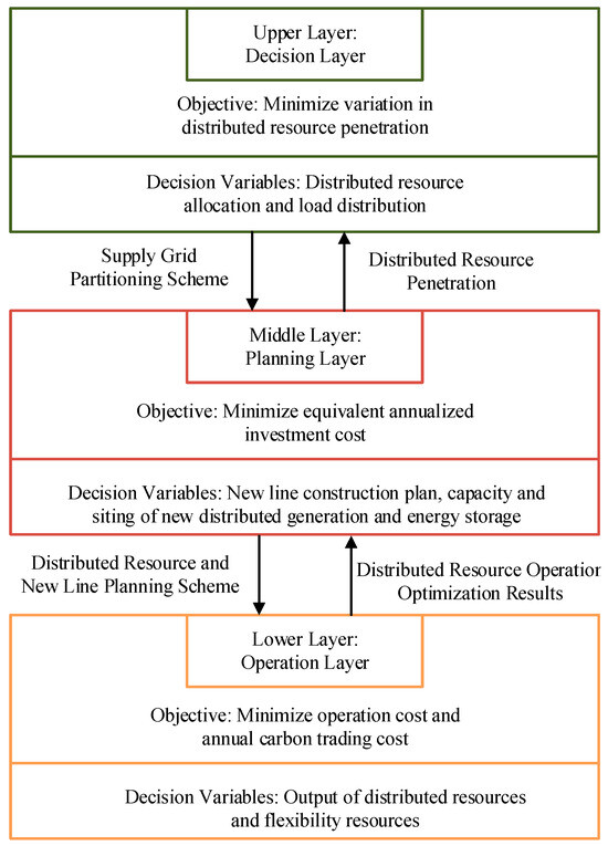
Figure 2.
Three-layer planning model of decision–planning–operation.
4.1. Decision Layer Model
4.1.1. Objective Function
(1) Deviation in Distributed Resource Penetration Rate:
where is the number of grids; denotes the power output of generation resources in the supply partition; is the active power of loads in the supply partition; represents the generation output in grid ; and denotes the active load power in grid .
(2) Distance Between Load Center and Generation Center:
where and represent the coordinates of the load center in grid ; and represent the coordinates of the generation center in grid .
4.1.2. Constraints
(1) Line Load Rate Constraint:
where and represent the line load rate and the maximum allowable line load rate, respectively.
(2) Supply Radius Constraint:
where and represent the supply radius of the substation and its maximum allowable value, respectively.
4.2. Planning Layer Model
4.2.1. Objective Function
Minimization of Equivalent Annualized Total Cost:
where denotes the equivalent annualized investment cost of new lines and represents the equivalent annualized investment cost of newly installed distributed generation (DG), with this study focusing on three types of DG: wind turbines, PV units, and gas turbines. stands for the equivalent annualized investment cost of newly added ESS. The detailed calculation formulas are as follows:
(1) Equivalent annualized investment cost of new lines
The equivalent annualized investment cost of new lines, denoted as , is expressed as Equation (18):
where is the line decision variable; when , the line is not planned; when , the line is planned. and represent the line’s investment return rate and annual operation and maintenance rate, respectively. denotes the annualized conversion coefficient of fixed investment costs. is the investment return rate; is the normal service life of the line; is the construction period. is the construction length of line ; is the unit length construction cost of line when the line type is . represents the entire set of lines that need to be constructed in the distribution network.
(2) Equivalent annualized investment cost of ESS
The equivalent annualized fixed investment and operation and maintenance cost of energy storage, denoted as , is expressed as follows:
where is the energy storage decision variable; when , no energy storage is allocated at the node; when , energy storage is allocated. and represent the investment return rate and annual operation and maintenance rate of energy storage, respectively. denotes the annualized conversion coefficient of the energy storage investment costs. is the rated capacity of energy storage connected at node ; is the unit capacity investment cost for energy storage of type at node . and are the annualized unit installation cost and unit operation and maintenance cost of energy storage, respectively. represents the set of planning nodes with allocated energy storage in the distribution network structure.
(3) Equivalent annualized investment cost of DG
The equivalent annualized fixed investment and operation and maintenance cost of DG are expressed as follows:
where denotes the type of DG connected at node ; indicates that no DG is connected at this node; indicates that the first, second, or third type of DG is connected, referring to wind turbines, PV units, and gas turbines in this study. Different values of the variable represent different DG types. and represent the DG investment return rate and annual operation and maintenance rate, respectively. is the annualized conversion coefficient of the DG investment costs. is the rated capacity of DG connected at node ; is the unit capacity investment cost of DG type connected at node . and are the unit installation cost and annual operation and maintenance cost of DG type connected at node , respectively. Different DG types have different unit installation and operation costs. Additionally, when , . represents the set of planning nodes with DG integration in the distribution network.
This study assumes that the performance degradation of PV, wind, and ESS within the planning horizon is implicitly accounted for through the discount factor embedded in the investment cost. The potential impact of explicitly modeling the degradation of these devices is not considered in this work.
4.2.2. Constraints
(1) Capacity Constraint of Proposed Gas Turbine Units:
where and represent the upper and lower capacity limits of the proposed gas turbine units, respectively.
(2) Capacity Constraint of Proposed ESS:
where and represent the upper and lower limits of the proposed energy storage capacity, respectively.
(3) Capacity Constraint of Proposed DG:
where and represent the upper and lower limits of the proposed DG capacity, respectively.
4.3. Lower-Level Operation Model
4.3.1. Objective Function
The lower level aims to minimize the sum of the annual operation cost and annual carbon trading cost , as expressed in Equation (24):
where the annual operation cost includes the gas turbine generation cost , the penalty cost for insufficient system flexibility , and the penalty cost for wind and solar curtailment . , , and are the coefficients of the gas turbine generation cost. is the penalty cost per unit of curtailed renewable generation. is the penalty cost per unit of flexibility shortfall. denotes the number of typical scenarios; is the number of days in typical scenario . represents the set of renewable units, including wind turbines and PV units. and are the actual output power and the maximum available power of renewable unit at time , respectively.
4.3.2. Constraints
(1) Gas Turbine Output Constraint:
where and represent the upper and lower output limits of the gas turbine units, respectively.
(2) DG Operation Constraints:
where , , , and represent the lower and upper limits of the active and reactive power output of the DG at node during time period under scenario , respectively.
(3) ESS Operation Constraints:
where and denote the maximum discharging and charging power of the energy storage, respectively; and are binary variables that indicate the discharging and charging states of the storage, with 1 representing discharging (or charging); , , and represent the SoC of the energy storage, and its lower and upper limits, respectively, at node during time period under scenario ; and denote the discharging and charging efficiencies; is the duration of time period ; and are the initial and final SoC at the start and end of operation, respectively.
(4) Power Flow Constraints of the System:
where is the set of sending-end nodes of branches for which node is the receiving end; is the set of receiving-end nodes of branches for which node is the sending end. , , and denote the resistance, reactance, and impedance of line , respectively. and represent the active and reactive power flows through the line at time under scenario . and denote the voltage magnitudes at nodes and , respectively. is the current magnitude of line . and are the active and reactive power injected at node . and represent the discharging and charging power of the ESS at node . , , and are the initial active power load, interruptible load, and transferable load at node , respectively. , , and denote the reactive power of the thermal units, that of the DG units, and the initial reactive load at node , respectively.
(5) Renewable Energy Utilization Constraint:
where denotes the threshold of renewable energy utilization.
(6) System Operational Security Constraints:
where is the voltage magnitude at node at time under scenario ; and represent the lower and upper bounds of the voltage magnitude, respectively; is the current magnitude of line at time under scenario ; and denotes the line’s current safety limit.
(7) Power Balance Constraint:
where is the output power of the gas turbine units; and are the output power of the PV and wind power units, respectively; is the output of the energy storage system; is the power purchased from the upstream grid; and is the total load demand.
5. Model Solution
5.1. Improved K-Means Algorithm
The K-means algorithm is a clustering method based on objective function optimization, and commonly uses Euclidean distance as the criterion for power supply grid division. However, Euclidean distance primarily emphasizes spatial proximity and does not account for the electrical coupling between distributed resources and loads, which can significantly affect grid partitioning [29]. To address this limitation in the context of SGLS coordinated planning in distribution networks, two evaluation indices—the electrical coupling degree and renewable energy accommodation rate—are introduced to comprehensively assess and optimize regional partitioning within the distribution system.
The comprehensive index system for regional division is primarily determined by the objectives and principles of distribution network partitioning. Considering the functional requirements of each region, this study develops an integrated evaluation framework to comprehensively assess and optimize regional partitioning. The system incorporates the electrical coupling degree, which reflects the electrical proximity between nodes; the voltage security margin, which indicates the overall deviation of node voltages during coordinated regulation; and the renewable energy accommodation rate, which evaluates the self-regulation capability of each region under partitioned conditions. The use of these indicators, together, aims to maximize the autonomy and operational efficiency of distribution network regions.
(1) Electrical Coupling Degree
In the architecture design of distribution networks, electrical connections between nodes within the same region are typically strong. The electrical coupling degree is quantified using the following formula:
where denotes the weight of the edge between nodes and , which is represented by the electrical distance between the two nodes; is half the sum of the weights of all edges within the region; represents the sum of the weights of all edges connected to node . If nodes and are located in the same region, then ; otherwise, .
(2) Voltage Security Margin
The voltage security margin is defined as the ability of PV, energy storage, and load resources within a region to regulate active and reactive power to control voltage deviations. The specific calculation formula is as follows:
where represents the voltage regulation capability index of region ; denotes the total number of partitioned regions; is the maximum voltage deviation of node within the region; and represents the maximum voltage regulation capacity at node , considering the active and reactive power margins within the region.
(3) Renewable Energy Accommodation Rate
The renewable energy accommodation rate refers to the ability of controllable sources and net load fluctuations within a region to be smoothed over the scheduling period. This metric helps evaluate and optimize the distribution network’s capacity for renewable energy integration and load regulation across different time intervals. The quantitative expression of this indicator is as follows:
where , , , and represent the adjustable capacities of distributed PV, wind power, energy storage, and flexible loads, respectively, as well as the net load within the region at time .
(4) Comprehensive Regional Partitioning Index System for Distribution Networks
Integrating the aforementioned regional division indicators and considering the regulation capabilities of the sources, loads, and storage within each region, the comprehensive partitioning index system for county-level distribution networks is formulated as follows to fully leverage regional autonomy.
where , , and are weighting coefficients, which satisfy the following condition:
The improved K-means algorithm is a hard clustering method based on a predefined number of clusters , with the following steps:
- Determine the number of clusters according to the prerequisites of grid partitioning;
- Define classification criteria using the spatiotemporal distances of load points and distributed resources;
- Calculate weights based on the comprehensive regional partitioning index; smaller weights indicate greater similarity between data points;
- Apply the minimum weight matching algorithm [30] to find the minimum weight set in the graph, and thereby group data points into distinct clusters;
- Use the K-means algorithm to separately select cluster centers and load centers.
Edges in the minimum weight matching connect vertices from different clusters, optimizing the matching between nearby cluster centers and load centers to determine the final grid partitioning results.
5.2. Search Method Based on Improved Adaptive Particle Swarm Optimization
Particle swarm optimization (PSO) treats the solution space of a problem as a multi-dimensional search space composed of particles. Each particle represents a potential solution and explores the space by adjusting its own position and velocity. The position of each particle is updated based on both its own best experience and the collective experience of the swarm, with the aim of identifying the optimal solution. Through continuous iterations, the swarm gradually converges toward the global optimum.
The steps of the IAPSO algorithm are as follows:
- Population Initialization
Initialize the velocity and position of all particles. Evaluate the objective function value for each particle.
- 2.
- Determination of Personal Best
During initialization, each particle’s personal best position is set to its current position.
- 3.
- Adaptive Inertia Weight Adjustment
In IAPSO, let the solution space be -dimensional (). Let and denote the velocity and position of each particle, respectively. Based on the current velocity and iteration index , the position of each particle is updated using the following equation:
For each particle, the velocity and position are updated using Equation (40). In this process, represents the particle’s personal best position, while denotes the global best position found by the entire population. The inertia weight serves to balance the global exploration and local exploitation capabilities. The acceleration coefficients and reflect the particle’s tendency to move toward its personal best and the global best positions, respectively. Additionally, and are uniformly distributed random numbers in the range [0, 1].
The inertia weight critically affects PSO’s search ability and convergence. Larger inertia weights favor global exploration, while smaller ones enhance local exploitation. Conventional PSO uses a fixed inertia weight, often resulting in suboptimal convergence. To improve the method’s stability and performance, this study employs an adaptive inertia weight that varies with each particle’s fitness. The update rules for minimization and maximization problems are given by Equations (41) and (42).
where and are the preset minimum and maximum inertia weight coefficients, is the fitness value of the particle at iteration , and are the minimum and maximum fitness values among all particles at iteration ttt, and is the average fitness of all particles at iteration . can be expressed as follows:
Taking the example of maximizing fitness using PSO, a higher fitness value indicates a better particle position. When a particle’s fitness is below the average fitness of all particles, it means that the particle is in a relatively poor position; in this case, setting the inertia weight to its maximum enhances the particle’s global search ability, helping it quickly move toward better regions. Conversely, when a particle’s fitness exceeds the average fitness, it indicates a relatively good position; adaptively reducing the inertia weight strengthens the particle’s local search ability, enabling faster convergence to the optimal solution. This inertia weight adjustment effectively balances global exploration and rapid convergence.
- 4.
- Adaptive Adjustment of Acceleration Factors
The acceleration factors and represent the cognitive ability of particles and their social information-sharing capability, respectively. Proper tuning of these factors can accelerate the search process and help avoid premature convergence to local optima. Therefore, this study improves the setting of acceleration factors and random constants , as shown in Equations (44) and (45):
In Equations (44) and (45), denotes the maximum number of iterations, the current iteration, and the inertia weight calculated by Equations (41) and (42); the other parameters share the same meaning as in Equation (40). This design allows particles to be influenced more by their individual best positions in early iterations, enabling rapid convergence to relatively good solutions. As the iterations progress, the influence of individual best positions diminishes, and particles move towards the global best, which promotes overall convergence.
Fixed inertia weights and acceleration coefficients often cause the algorithm to get trapped in local optima, reducing its optimization performance. Therefore, this study dynamically updates the acceleration coefficients based on the adaptive inertia weight, as shown in Equations (46) and (47).
Based on the adaptive inertia weight, the quality of each particle’s position is reflected, which allows appropriate adjustment of the particle’s cognitive and social sharing abilities so that particles can more rapidly converge toward their own historical best positions and the global best position.
- 5.
- Crossover and Mutation Operation
To generate new offspring, random values are drawn from a Gaussian distribution and added to components of the solution vector. This helps the algorithm escape local optima. For each parent solution vector, the offspring produced by Gaussian mutation at generation is expressed as follows:
where and represent the mean and standard deviation of the Gaussian distribution, respectively. denotes a Gaussian random variable with a mean of 0 and a standard deviation of 1. The standard deviation for each solution vector is calculated by Equation (49):
where is the fitness value of the solution in the population, and is the minimum fitness value among the current population’s solution vectors.
- 6.
- Calculate the fitness of each particle and update the individual best positions.
- 7.
- Check if the maximum number of iterations is reached. If yes, output the results; if not, return to step (3).
5.3. Solution Procedure
- Preprocess the planning of the power supply partitions, determine the optimal number of clusters, and use the improved K-means clustering algorithm to identify load centers and DG centers. Then, apply minimum weight matching to define the power supply grids. The grid partition results are passed to the middle layer;
- Initialize parameters of the IAPSO algorithm and generate the initial population;
- Pass the configuration scheme generated by the middle layer to the lower layer as the initial conditions. The lower layer model determines the economic operation cost and environmental governance cost based on distributed resource outputs, and thus identifies the optimal operational strategy for the grid;
- Pass the optimal strategy to the middle layer. If the DG penetration meets the requirements, do not return to the upper layer. The middle layer updates the global particle velocities and positions directly based on the optimized scheme;
- Check whether the termination condition is met. If yes, the global optimum is the optimal planning scheme; if not, update the particle positions and velocities and return to step 2.
6. Simulation Analysis
To verify the effectiveness of the proposed strategy, simulation experiments were conducted in MATLAB R2024a using the IEEE 33-bus distribution network as an example. The system base voltage is set to 12.66 kV, and the allowable voltage range at the nodes is [0.95 p.u., 1.05 p.u.]. The system is equipped with diesel generators, and the planned types of DG include wind turbines, PV, micro gas turbines, and energy storage devices. The rated capacity of a single DG unit is 50 kW. The unit investment costs per kW are 5000, 6500, 1500, and 2000 RMB for wind energy, PV energy, micro gas turbine energy, and energy storage, respectively; the unit maintenance costs are 0.06, 0.04, 0.04, and 0.05 RMB/kWh, respectively. The unit investment cost for lines is 150,000 RMB/km. The planning investment period is 10 years with a discount rate of 0.1. Each node can accommodate up to 10 units of wind turbines and PV devices. The state of charge (SOC) for the storage devices ranges from 0.1 to 0.9, and they have charge/discharge efficiencies of 0.9.
The electricity purchase prices are segmented as follows: off-peak hours 0:00–8:00 and 11:30–13:30 at 0.25 RMB/kWh; flat hours 8:00–11:30, 13:30–16:30, and 22:30–24:00 at 0.42 RMB/kWh; peak hours 16:30–20:30 at 0.65 RMB/kWh; and sharp peak hours 20:30–22:30 at 0.82 RMB/kWh. The initial carbon trading price is 400 RMB/ton. To ensure the rationality of the parameter settings, the investment and maintenance costs in this study are primarily derived from the relevant literature and typical data from the domestic renewable energy market. The time-of-use electricity prices are based on the pricing structures of regional electricity markets, and the carbon trading price is taken from the recent average market level. These parameters are selected to establish a representative simulation environment for validating the proposed model and methodology.
The partitioning results of the IEEE 33-node network and the line construction plan are shown in Figure 3. The wind power output and load variation curves for four typical days are shown in Figure 4.
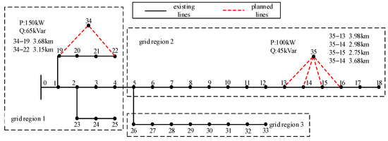
Figure 3.
Schematic diagram and zoning results of the IEEE 33-bus distribution network.
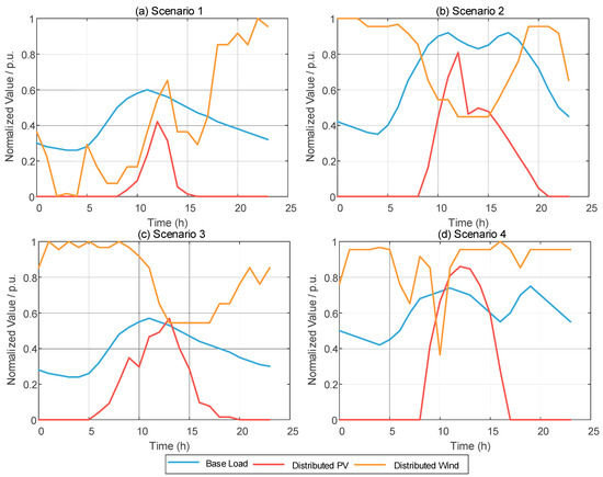
Figure 4.
Wind power output and load variation curves on typical days.
6.1. Planning Results Analysis
The planning scheme obtained using the IAPSO is presented in Table 1.

Table 1.
33-node distribution network planning scheme.
The configuration results indicate that, due to the uncertainty of distributed resources, the planning tends to deploy them in load-intensive areas to achieve local consumption. Considering the variability of PV generation, energy storage devices are preferably allocated in regions with a high concentration of distributed PV units. Through charging and discharging, they help smooth peak loads and valleys, thereby enhancing the stability of the distribution network.
Next, the impact of carbon trading prices on the planning results is analyzed. Under the conditions that the lengths of the positive and negative carbon emission intervals and the carbon quota purchase cost growth coefficient remain unchanged, the electricity–carbon coupling market is considered. The carbon trading price is varied within the range of 0 to 600 RMB/t, and the configuration results of gas turbines, wind power, PV energy, and ESS are shown in Figure 5.
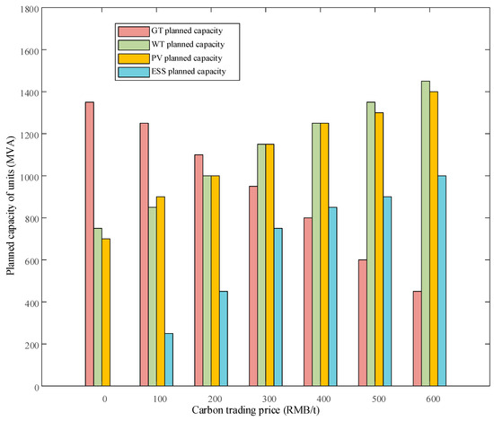
Figure 5.
Configuration results under different carbon trading prices.
As the carbon trading price increases, the capacity of the gas turbine units gradually decreases, while the capacities of the DERs and ESS steadily increase. This indicates that higher carbon prices lead to greater carbon emission costs, prompting an expansion in the installed capacity of renewable energy and pure energy systems to reduce system emissions and, consequently, carbon trading costs. With further increases in carbon prices, these capacities approach their respective limits.
6.2. Analysis of Advantages of the IAPSO
The initial parameters of the IAPSO algorithm are configured as follows: the population size is set to 80, and the maximum number of iterations is 100. A constraint is imposed to ensure that the power generation from DERs accounts for more than 50% of the total generation. Taking the total system cost as an example, the convergence curves of the standard PSO algorithm and the IAPSO algorithm are illustrated in Figure 6.
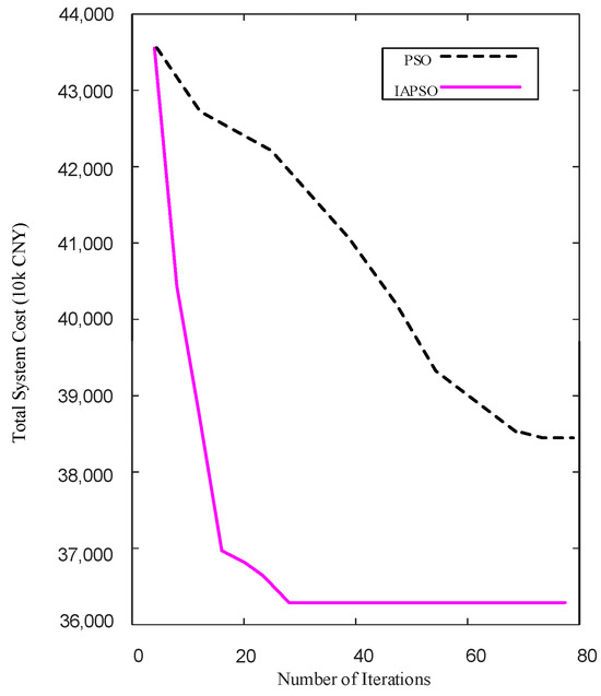
Figure 6.
Iterative convergence curves.
As shown in the figure, the IAPSO algorithm outperforms the traditional PSO in both convergence speed and convergence quality. The improved algorithm converges in about 28 iterations, whereas the traditional PSO requires approximately 70 iterations to reach convergence.
To more clearly demonstrate the advantages of the IAPSO algorithm, this study compares it with the standard PSO and the traditional genetic algorithm (GA), as well as differential evolution (DE) [31] and the grey wolf optimizer (GWO) [32]. The planning results for the investment and operational costs obtained by these methods are summarized in Table 2.
Table 2.
Cost calculation results of planning using three methods.
As shown in Table 2, the planning scheme based on IAPSO outperforms PSO, the GA, DE, and the GWO across all cost metrics, including investment and operation cost, curtailment penalty, flexibility penalty, carbon trading cost, and total system cost. This advantage arises from three key enhancements in the IAPSO framework. First, the inertia weight is dynamically adjusted based on particle fitness—particles with lower fitness are assigned larger inertia weights to enhance global exploration, while those with better performance receive smaller weights to refine their local search. Second, the acceleration coefficients evolve adaptively throughout the iterations, emphasizing individual cognition in the early stages for rapid exploration and gradually strengthening social collaboration to improve the convergence speed. Third, a Gaussian mutation mechanism is incorporated to increase solution diversity and help the population escape local optima. These combined mechanisms enable IAPSO to achieve faster convergence and more accurate global optimization results, ultimately leading to a more cost-effective planning outcome.
6.3. Analysis of Power Supply Zone Operation
The optimal operation strategies for the three power supply zones on a typical day, derived from the proposed planning scheme, are illustrated in Figure 7, Figure 8 and Figure 9.
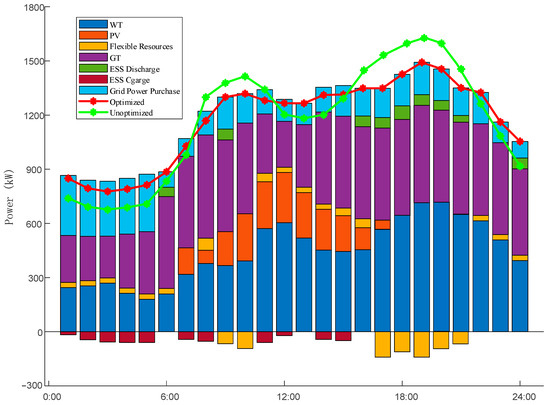
Figure 7.
Typical daily operation of Power Supply Zone 1.
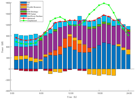
Figure 8.
Typical daily operation of Power Supply Zone 2.
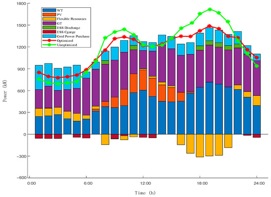
Figure 9.
Typical daily operation of Power Supply Zone 3.
Based on the typical daily operation profiles of each power supply zone, the system charges energy storage devices when wind and solar outputs are high, and discharges them during peak demand periods to supply power to the grid. During off-peak hours, electricity is purchased from the grid while the storage units are charged simultaneously. This strategy enables the local consumption of DERs and minimizes operational costs by leveraging time-of-use electricity pricing. In addition, flexible resources, such as shiftable loads, are utilized to further flatten the peak demand and fill valleys.
6.4. Analysis of Planning Results Under Different Scenarios
To more clearly compare and analyze the impacts of considering electricity–carbon coupling and flexibility supply–demand balance on the coordinated planning of SGLS, this study designs four different planning scenarios for validation and comparison:
- Scenario 1: Planning considering only time-of-use electricity pricing;
- Scenario 2: Planning considering electricity–carbon coupling;
- Scenario 3: Planning considering flexibility supply–demand balance.
- Scenario 4: Planning considering both electricity–carbon coupling and flexibility supply–demand balance.
The cost planning results of the three scenarios are shown in Table 3.
Table 3.
Cost calculation results of planning under four scenarios.
Scenario 1, which only considers the electricity pricing mechanism, leads to the highest overall cost, with pronounced flexibility penalties and renewable curtailment. Scenario 2 introduces electricity–carbon coupling, effectively reducing curtailment and carbon trading costs while improving the utilization of distributed resources. Scenario 3 incorporates a flexibility supply–demand balancing mechanism, which further alleviates flexibility shortages and enhances the system’s efficiency. Scenario 4 combines electricity–carbon coupling with flexibility balancing, achieving the best performance in terms of cost reduction, renewable energy integration, and system flexibility and thereby providing a comprehensive and economically efficient solution for modern power system planning.
6.5. Method Consistency Test
Without altering the parameters of the simulation model, the proposed planning method was executed 30 independent times. The resulting new line construction plans and distributed generation configurations were completely identical across all runs. The standard deviation of the total cost obtained from the 30 independent runs was less than 1.4%, whereas the standard deviations for the traditional PSO and GA methods were approximately 4.5% and 5.2%, respectively. These results demonstrate the strong consistency and robustness of the proposed method.
6.6. Validation on a Larger-Scale Network
To further verify the effectiveness of the proposed method, the more complex PG&E 69-bus distribution system [33] was tested. The parameter settings were kept consistent with those described in this section. The partitioning results of the 69-bus system and the corresponding line construction plans are shown in Figure 10.
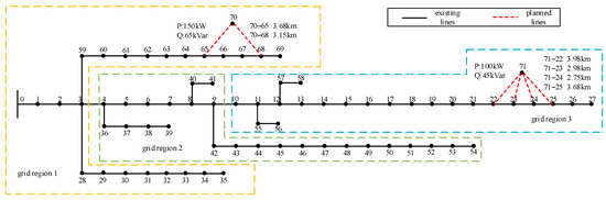
Figure 10.
Schematic diagram and zoning results of the PG&E 69-bus distribution network.
The planning scheme obtained using the IAPSO algorithm is presented in Table 4.
Table 4.
69-node distribution network planning scheme.
From the configuration results, it can be observed that, for the 69-bus network, the proposed method still provides an effective planning scheme. Considering the uncertainty of distributed resources, the method tends to allocate them in load-intensive areas to achieve local consumption. These results confirm that the proposed method remains effective and applicable to larger-scale distribution networks.
6.7. Discussion
The simulation results provide several important insights into the effectiveness of the proposed model and the IAPSO algorithm.
First, the integration of the electricity–carbon coupling mechanism substantially improves the planning performance. By establishing a linkage between electricity prices and carbon trading signals, the model creates a coordinated market environment that guides investment towards low-carbon resources while discouraging carbon-intensive generation. This mechanism not only promotes the utilization of renewable energy but also contributes to the reduction of overall system costs through the mitigation of carbon-related expenditures.
Second, the incorporation of a flexibility supply–demand balancing framework proves to be essential for ensuring the secure and economic operation of the system. The explicit quantification of flexibility and the coordinated scheduling of multiple resources, including energy storage and controllable loads, enable the model to effectively accommodate renewable variability. This reduces dependence on conventional thermal generation for balancing purposes and alleviates operational stress, thereby improving both economic efficiency and system reliability.
Third, the proposed IAPSO algorithm exhibits superior convergence performance and robustness relative to conventional metaheuristic approaches. The adaptive adjustment of its parameters and the introduction of Gaussian mutation enhance its global exploration capability while maintaining solution diversity, which ensures stable and high-quality optimization results across repeated runs.
Finally, the successful application of the proposed approach to a larger-scale distribution network validates its scalability and practical applicability. This indicates that the model and algorithm are suitable for complex real-world systems. Future research may extend this work by explicitly modeling equipment degradation and incorporating more detailed representations of demand-side flexibility, thus further improving the accuracy and applicability of the proposed framework.
7. Conclusions
This study proposes a three-layer coordinated planning model for source–grid–load–storage systems considering electricity–carbon coupling and flexibility supply–demand balance. The key contributions and findings can be summarized as follows:
- The proposed “Decision–Planning–Operation” structure provides a systematic approach for distribution network planning. By combining grid partitioning, coordinated resource allocation, and multi-scenario operational optimization, the model effectively reduces planning complexity while enhancing cost efficiency and renewable energy integration;
- The improved adaptive IAPSO algorithm demonstrates faster convergence and higher solution accuracy compared with conventional metaheuristic techniques, offering robust computational support for large-scale and highly constrained planning problems;
- The introduction of a dynamic electricity–carbon pricing mechanism effectively promotes the deployment of low-carbon resources and reduces the total system cost, supporting the low-carbon transition of distribution networks;
- By quantifying and coordinating the flexibility contributions of conventional units, energy storage, and controllable loads, the model mitigates flexibility shortages, reduces renewable curtailment, and alleviates the over-reliance on thermal units, thereby improving system operational reliability and economic performance.
These results confirm the scalability and practical applicability of the proposed model and algorithm, providing a feasible solution for future low-carbon and flexibility-oriented distribution network planning. Future work will focus on incorporating equipment degradation and more detailed demand-side flexibility models to further enhance planning accuracy.
In addition, this study contributes to sustainable development by integrating economic, environmental, and operational objectives into a unified planning framework. By promoting the deployment of renewable energy, reducing carbon emissions, and enhancing the efficiency of flexibility resource utilization, the proposed model supports the transition towards cleaner and more resilient energy systems. This aligns with global sustainability goals and provides actionable insights for policymakers and utilities seeking to achieve both economic efficiency and environmental responsibility in power system planning.
Author Contributions
Conceptualization, Z.W., H.C. and Z.H.; Methodology, Z.W. and H.T.; Software, Z.W. and L.Z.; Validation, H.C. and H.T.; Investigation, L.Z.; Resources, J.Z. and Z.L.; Writing—Original Draft, Z.W., H.C. and H.T.; Visualization, Z.W.; Supervision, Z.H.; Project administration, Z.H.; Funding acquisition, J.Z. and Z.L. All authors have read and agreed to the published version of the manuscript.
Funding
The authors declare that this study received funding from The Science and Technology Project of Guangdong Power Grid Corporation, Foshan Power Sup-ply Bureau of Guangdong Power Grid Corporation (030600KC23100019). The funder was not involved in the study design, collection, analysis, interpretation of data, the writing of this article or the decision to submit it for publication.
Institutional Review Board Statement
Not applicable.
Informed Consent Statement
Not applicable.
Data Availability Statement
Data sharing is available by emailing the corresponding author.
Conflicts of Interest
Authors Jianfeng Zheng and Zhilu Liu were employed by the company Foshan Power Supply Bureau of Guangdong Power Grid Corporation. The remaining authors declare that the research was conducted in the absence of any commercial or financial relationships that could be construed as a potential conflict of interest.
Abbreviations
The following abbreviations are used in this manuscript:
| Abbreviations | |
| SGLS | Source–grid–load–storage |
| IAPSO | Improved adaptive particle swarm optimization |
| PSO | Particle swarm optimization |
| GA | Genetic Algorithm |
| PV | Photovoltaic |
| WT | Wind power |
| GT | Gas turbines |
| ESS | Energy storage systems |
| DG | Distributed generation |
| DERs | Distributed energy resources |
| Variables | |
| Average carbon price | |
| Total carbon emissions traded on the previous day | |
| Tiered carbon price | |
| Carbon emission cost | |
| Upward and downward flexibility of conventional unit | |
| Upward and downward flexibility provided by energy storage | |
| Upward flexibility provided by shiftable loads and interruptible loads | |
| Downward flexibility of shiftable loads | |
| Equivalent annualized investment cost of new lines, DG, and ESS | |
| Annual operation cost | |
| Gas turbine generation cost | |
| Penalty cost for insufficient system flexibility | |
| Penalty cost for wind and solar curtailment | |
References
- Wang, Z.; Bu, S.; Wen, J.; Huang, C. A Comprehensive Review on Uncertainty Modeling Methods in Modern Power Systems. Int. J. Electr. Power Energy Syst. 2025, 166, 110534. [Google Scholar] [CrossRef]
- Farokhzad Rostami, H.; Samiei Moghaddam, M.; Radmehr, M.; Ebrahimi, R. Energy Expansion Planning with a Human Evolutionary Model. Energy Inform. 2024, 7, 64. [Google Scholar] [CrossRef]
- Zhu, Y.; Li, D.; Xiao, S.; Liu, X.; Bu, S.; Wang, L.; Ma, K.; Ma, P. Coordinated Control Strategy of Source-Grid-Load-Storage in Distribution Network Considering Demand Response. Electronics 2024, 13, 2889. [Google Scholar] [CrossRef]
- Zubo, R.H.A.; Mokryani, G.; Rajamani, H.-S.; Aghaei, J.; Niknam, T.; Pillai, P. Operation and Planning of Distribution Networks with Integration of Renewable Distributed Generators Considering Uncertainties: A Review. Renew. Sustain. Energy Rev. 2017, 72, 1177–1198. [Google Scholar] [CrossRef]
- Zhang, Y.; Liang, C.; Wang, H.; Zhang, J.; Zeng, B.; Liu, W. A Multi-Objective Interval Optimization Approach to Expansion Planning of Active Distribution System with Distributed Internet Data Centers and Renewable Energy Resources. IET Gener. Transm. Distrib. 2024, 18, 2999–3016. [Google Scholar] [CrossRef]
- Mao, J.; Jafari, M.; Botterud, A. Planning Low-Carbon Distributed Power Systems: Evaluating the Role of Energy Storage. Energy 2022, 238, 121668. [Google Scholar] [CrossRef]
- Majzoobi, A.; Khodaei, A.; Bahramirad, S. Capturing Distribution Grid-Integrated Solar Variability and Uncertainty Using Microgrids. In Proceedings of the 2017 IEEE Power & Energy Society General Meeting, Chicago, IL, USA, 16–20 July 2017. [Google Scholar]
- Yang, J.; Zhang, N.; Botterud, A.; Kang, C. Situation Awareness of Electricity-Gas Coupled Systems with a Multi-Port Equivalent Gas Network Model. Appl. Energy 2020, 258, 114029. [Google Scholar] [CrossRef]
- Wu, Q.-H.; Bose, A.; Singh, C.; Chow, J.H.; Mu, G.; Sun, Y.; Liu, Z.; Li, Z.; Liu, Y. Control and Stability of Large-Scale Power System with Highly Distributed Renewable Energy Generation: Viewpoints from Six Aspects. CSEE J. Power Energy Syst. 2023, 9, 8–14. [Google Scholar] [CrossRef]
- Gao, C.; Lu, H.; Chen, M.; Chang, X.; Zheng, C. A Low-Carbon Optimization of Integrated Energy System Dispatch under Multi-System Coupling of Electricity-Heat-Gas-Hydrogen Based on Stepwise Carbon Trading. Int. J. Hydrogen Energy 2025, 97, 362–376. [Google Scholar] [CrossRef]
- Xue, K.; Wang, J.; Hu, G.; Wang, S.; Zhao, Q.; Chong, D.; Yan, J. Optimal Planning for Distributed Energy Systems with Carbon Capture: Towards Clean, Economic, Independent Prosumers. J. Clean. Prod. 2023, 414, 137776. [Google Scholar] [CrossRef]
- Ba-swaimi, S.; Verayiah, R.; Ramachandaramurthy, V.K.; ALAhmad, A.K.; Padmanaban, S. Optimal Planning of Renewable Distributed Generators and Battery Energy Storage Systems in Reconfigurable Distribution Systems with Demand Response Program to Enhance Renewable Energy Penetration. Results Eng. 2025, 25, 104304. [Google Scholar] [CrossRef]
- Liu, X. Strategy Research on Variable Load Carbon Price and Demand Response of Integrated Energy System Based on Stackelberg Game and Cooperative Game. Energy 2025, 328, 136579. [Google Scholar] [CrossRef]
- Zhang, Y.; Ge, X.; Li, M.; Li, N.; Wang, F.; Wang, L.; Sun, Q. Demand Response Potential Day-Ahead Forecasting Approach Based on LSSA-BPNN Considering the Electricity-Carbon Coupling Incentive Effects. IEEE Trans. Ind. Appl. 2024, 60, 4505–4516. [Google Scholar] [CrossRef]
- Hua, H.; Chen, X.; Gan, L.; Sun, J.; Dong, N.; Liu, D.; Qin, Z.; Li, K.; Hu, S. Demand-Side Joint Electricity and Carbon Trading Mechanism. IEEE Trans. Ind. Cyber-Phys. Syst. 2024, 2, 14–25. [Google Scholar] [CrossRef]
- Lu, X.; Qiu, J.; Lei, G.; Zhu, J. An Interval Prediction Method for Day-Ahead Electricity Price in Wholesale Market Considering Weather Factors. IEEE Trans. Power Syst. 2024, 39, 2558–2569. [Google Scholar] [CrossRef]
- Lu, X.; Qiu, J.; Yang, Y.; Zhang, C.; Lin, J.; An, S. Large Language Model-Based Bidding Behavior Agent and Market Sentiment Agent-Assisted Electricity Price Prediction. Policy Regul. IEEE Trans. Energy Mark. 2025, 3, 223–235. [Google Scholar] [CrossRef]
- Rahman, M.M.; Dadon, S.H.; He, M.; Giesselmann, M.; Hasan, M.M. An Overview of Power System Flexibility: High Renewable Energy Penetration Scenarios. Energies 2024, 17, 6393. [Google Scholar] [CrossRef]
- Mohandes, B.; Moursi, M.S.E.; Hatziargyriou, N.; Khatib, S.E. A Review of Power System Flexibility with High Penetration of Renewables. IEEE Trans. Power Syst. 2019, 34, 3140–3155. [Google Scholar] [CrossRef]
- Zhao, Y.; Hu, S.; Wang, Y.; Cao, L.; Yang, J. Assessing Flexibility by Ramping Factor in Power Systems with High Renewable Energy Proportion. Int. J. Electr. Power Energy Syst. 2024, 155, 109680. [Google Scholar] [CrossRef]
- Impram, S.; Varbak Nese, S.; Oral, B. Challenges of Renewable Energy Penetration on Power System Flexibility: A Survey. Energy Strategy Rev. 2020, 31, 100539. [Google Scholar] [CrossRef]
- Wang, C.; Liu, C.; Zhou, X.; Zhang, G. Flexibility-Based Expansion Planning of Active Distribution Networks Considering Optimal Operation of Multi-Community Integrated Energy Systems. Energy 2024, 307, 132601. [Google Scholar] [CrossRef]
- Lu, Z.; Li, H.; Qiao, Y. Probabilistic Flexibility Evaluation for Power System Planning Considering Its Association with Renewable Power Curtailment. IEEE Trans. Power Syst. 2018, 33, 3285–3295. [Google Scholar] [CrossRef]
- Li, H.; Lu, Z.; Qiao, Y. Flexibility Resource and Demand Balance Mechanism in Power System Planning Considering High Penetration of Renewable Energy. In Proceedings of the 2017 IEEE Power & Energy Society General Meeting, Chicago, IL, USA, 16–20 July 2017. [Google Scholar]
- Li, X.; Qian, J.; Yang, C.; Chen, B.; Wang, X.; Jiang, Z. New Power System Planning and Evolution Path with Multi-Flexibility Resource Coordination. Energies 2024, 17, 273. [Google Scholar] [CrossRef]
- Liu, J.; Guo, T.; Wang, Y.; Li, Y.; Xu, S. Multi-Technical Flexibility Retrofit Planning of Thermal Power Units Considering High Penetration Variable Renewable Energy: The Case of China. Sustainability 2020, 12, 3543. [Google Scholar] [CrossRef]
- Chen, Z.; Hu, Y.; Tai, N.; Tang, X.; You, G. Transmission Grid Expansion Planning of a High Proportion Renewable Energy Power System Based on Flexibility and Economy. Electronics 2020, 9, 966. [Google Scholar] [CrossRef]
- Gonzalez-Salazar, M.A.; Kirsten, T.; Prchlik, L. Review of the Operational Flexibility and Emissions of Gas- and Coal-Fired Power Plants in a Future with Growing Renewables. Renew. Sustain. Energy Rev. 2018, 82, 1497–1513. [Google Scholar] [CrossRef]
- Zhao, C.; Zhao, J.; Wu, C.; Wang, X.; Xue, F.; Lu, S. Power Grid Partitioning Based on Functional Community Structure. IEEE Access 2019, 7, 152624–152634. [Google Scholar] [CrossRef]
- Rosato, F. Heuristic Graph Partitioning with Preferred Cluster Sizes and Application to the Generation of Realistic Distribution Grid Topologies. In Proceedings of the 2021 IEEE 15th International Conference on Compatibility, Power Electronics and Power Engineering (CPE-POWERENG), Florence, Italy, 14–16 July 2021; pp. 1–7. [Google Scholar]
- Han, J.; Feng, X.; Chen, Z.; Hu, P.; Zhao, H.; Chen, Y.; Liu, N. An Evolutionary Planning Method for Distribution Networks Considering Prosumers and Shared Energy Storage. Front. Energy Res. 2024, 12, 1298226. [Google Scholar] [CrossRef]
- Ansari, M.M.; Guo, C.; Shaikh, M.S.; Chopra, N.; Haq, I.; Shen, L. Planning for Distribution System with Grey Wolf Optimization Method. J. Electr. Eng. Technol. 2020, 15, 1485–1499. [Google Scholar] [CrossRef]
- Moghaddam, M.J.H.; Kalam, A.; Shi, J.; Nowdeh, S.A.; Gandoman, F.H.; Ahmadi, A. A New Model for Reconfiguration and Distributed Generation Allocation in Distribution Network Considering Power Quality Indices and Network Losses. IEEE Syst. J. 2020, 14, 3530–3538. [Google Scholar] [CrossRef]
Disclaimer/Publisher’s Note: The statements, opinions and data contained in all publications are solely those of the individual author(s) and contributor(s) and not of MDPI and/or the editor(s). MDPI and/or the editor(s) disclaim responsibility for any injury to people or property resulting from any ideas, methods, instructions or products referred to in the content. |
© 2025 by the authors. Licensee MDPI, Basel, Switzerland. This article is an open access article distributed under the terms and conditions of the Creative Commons Attribution (CC BY) license (https://creativecommons.org/licenses/by/4.0/).