Abstract
The rise in global supply chain pressure (GSCP) not only disturbs global sustainable development but also affects commodity prices. In this study, taking crude oil as an example, we use data from 1998 to 2024 and employ a structural VAR model to explore this effect. The empirical findings reveal that after a positive GSCP shock, crude oil prices rose immediately before the outbreak of global trade tensions in 2018. After 2018, however, prices decreased initially and then increased again about two months later. This response heterogeneity is primarily related to differences in the key drivers of GSCP between two periods.
1. Introduction
The high efficiency and low cost of the global supply chain are crucial for the operation of global business, including international trade, international investment, the operation of multinational enterprises, and global sustainable growth. However, there have been frequent natural and anthropogenic disturbances to the global supply chain. In particular, since the emergence of global trade tensions brought about by the US–China trade war, and the sudden outbreak of the COVID-19 pandemic, the industrial and supply chains have been distorted or interrupted, and transportation costs have risen compared with their trend value. For example, according to the global supply chain pressure index (GSCP index) established by Benigno et al. [1] (see Figure 1), the state of the global supply chain remained relatively stable before 2018 but has fluctuated considerably since then, and the value of the index peaked during the COVID-19 pandemic. Some researchers attribute the high inflation during and after the COVID-19 pandemic to such pressures, as the distortion in the supply chain has indeed increased the cost of many tradable goods [2]. Studies also demonstrate that both COVID-19 and the Russia–Ukraine conflict significantly increased food prices in the EU [3]. As a major tradable good and one of the most important commodities in the world, the refiner acquisition cost of crude oil is closely related to global shipping and transportation costs, which are also linked to the state of the global supply chain. In addition to this direct channel, the movement of global supply chain pressure may also trigger a change in the demand for crude oil, production adjustment, and speculative activity in futures markets, thereby forming indirect channels. Thus, the following question arises: how does the price of crude oil respond to a shock in GSCP? Furthermore, since the key driving factors behind the movement of the GSCP index are time-varying, another question arises: is the response of crude oil prices to a GSCP shock related to the characteristics of drivers of GSCP movements?
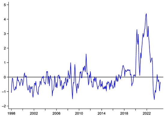
Figure 1.
The evolution of the GSCP index. Source: https://www.newyorkfed.org/research/policy/gscpi#/interactive (accessed on 1 January 2025); please see the website for more information on the GSCP index.
This study aims to answer the above questions. We argue that the channels through which a GSCP shock impact the futures price of crude oil can be classified into two categories: (1) Direct channels: An increase in the GSCP index increases shipping costs, which, in turn, directly increases the refiner acquisition cost of crude oil. The construction of the GSCPI incorporates transportation price indices, such as the Baltic Dry Cargo Index (BDI), the Harpex Index, and airfreight cost indices from the U.S. Bureau of Labor Statistics. (2) Indirect channels: A GSCP shock can influence the key driving factors for the movement of crude oil prices, such as global demand and production, speculation in futures markets, the risk-free rate, and the risk premium in financial markets. These factors, in turn, affect crude oil prices through various mediating mechanisms (see Figure 2). We then conduct an empirical analysis using a structural VAR (SVAR) model, and the empirical results show that, over the full sample period, a rise in the GSCP index slightly but significantly reduces crude oil prices initially, followed by an increase after a few months. At first glance, this pattern may appear counterintuitive. However, a comparative analysis demonstrates that the responses of crude oil prices and other mediating variables to GSCP shock were quite different before and after the outbreak of global trade tensions in 2018. Specifically, in the pre-2018 period, a positive GSCP shock immediately raise crude oil prices. In contrast, in the post-2018 period, prices initially decreased after the shock and then increased about two months later. We argue that such differences originate from the difference in the key driving factors for the movement of the GSCP index across the two periods. In particular, during the second period, the surge in the GSCP index was triggered by global trade tensions and the lockdown policy during the COVID-19 pandemic. Disruptions in the global supply chain during this time would have significantly impacted the risk appetite of investors, industrial output, and crude oil production, thereby influencing crude oil prices. In contrast, in the first period, the GSCP index remained relatively stable, and its impact on other variables was negligible.
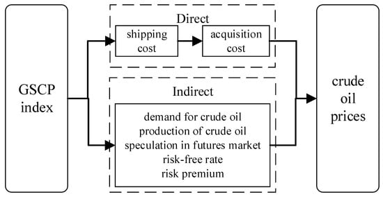
Figure 2.
Transmission channels of GSCP shocks affecting crude oil prices.
This study is related to emerging literature on the impact of global supply chain disruptions. Some studies have verified that global supply chain disruptions in could negatively impact macroeconomic outcomes and are associated with lower outputs and high inflation [2,4,5,6]. For example, Finck and Tillman [7] find that global supply chain shock causes a drop in economic activity in the European area and an increment in consumer prices, while Diaz et al. [4] show that global supply chain disruptions exacerbated inflation in four industrialized countries after the outbreak of COVID-19 pandemic. Another branch of the literature focuses on whether global supply chain disruptions impact financial markets. Ginn [6] reveals that supply chain shocks can lower global equity returns, while other studies investigate which kinds of financial asset—such as precious metals, cryptocurrency, renewable stock or green bonds [8,9,10,11]—can hedge against global supply chain pressure; however, no consensus has been reached. Two studies that align with ours in terms of scope are Rajput et al. [12] and Gozgor et al. [13]; the former demonstrates that the price volatility in commodity markets increased during the COVID-19 pandemic, while the latter reveals that global supply chain pressure has negative impacts on commodities, with the agriculture, food, and non-energy markets representing net transmitters of these shocks. However, neither of these articles discuss the differences in these impacts between periods while considering various driving factors of GSCP shocks.
The contributions of this study are threefold. First, we provide new insights into the effects of global supply chain disruption on the price of commodities in futures markets. It is logical to assume that a rise in transportation costs triggered by global supply chain disruption would increase the price of crude oil due to the isolation of production, refinery, and consumption, but this assumption is static and incomplete; in this era characterized by the financialization of commodities and globalization, the price of crude oil is affected by many other factors that place pressure on the global supply chain. Though a few studies have focused on the effect of global supply chain disruption on commodity markets, further investigations are required to thoroughly analyze this effect.
Second, we discuss the heterogeneous reactions of crude oil prices to GSCP shocks in different periods while considering various driving factors. In particular, we find that after the outbreak of global trade tensions in 2018, crude oil prices were depressed initially, and then rebounded about 2 months later after a positive GSCP shock; these results are quite different from those obtained before 2018. Therefore, we reveal that the time-varying nature of the impact of GSCP shock on commodity prices is contingent upon the key driving factors behind the movement of the GSCP index, which has important implications for investors. For example, investors should not expect a unidimensional linear response to GSCP shocks, and should conduct granular analyses of their underlying drivers.
Third, taking crude oil as an example, the findings of this study provide policymakers with an empirically grounded decision-making reference for stabilizing energy markets and meeting the Sustainable Development Goals (SDGs). Indeed, global supply chain disruptions not only reduce demand and output and threaten sustainable development, but also induce excessive volatility in energy and commodity prices, which may be detrimental for energy users and producers. Therefore, international cooperation is needed to avoid or alleviate supply chain disruptions.
The remainder of this paper is organized as follows: Section 2 introduces the variables, data, and specification of the empirical model, and Section 3 presents the results of the empirical and comparative analyses. In Section 4, we investigate the exact factors which drive the movement of the GSCP index; Section 5 presents the results of the robustness test; and finally, Section 6 presents our conclusions.
2. Variables and Model Specification
2.1. Empirical Model and Selection of Variables
Following the method of Baumeister and Hamilton [14] and Kilian and Zhou [15], we used the SVAR model to assess the impact of global supply chain shocks on crude oil prices in futures markets. Our SVAR model was set as follows:
where represents a vector of serially uncorrelated errors. The reduced-form error can be decomposed to .
represents the global supply chain pressure index for period , measured using standard deviations from its historical average, for which the data was sourced from the Federal Reserve Bank of New York website. In their study, Benigno et al. [1] collected two sets of indicators: the first focuses on cross-border transportation costs (including the Baltic Dry Index, Harpex index, and outbound and BLS airfreight price indices), and the second relies on country-level manufacturing data from the Purchase Managers’ Index (PMI) surveys. Then, they estimated a common, or “global”, component from these indicators and extracted it through principal component analysis, using it to fill the data gaps.
represents the CBOE Implied Volatility Index, which is widely used to determine market sentiment. Robe and Wallen [16], among many other scholars, show that the implied volatilities of crude oil options are driven in part by VIX, and Adrian and Shin [17] indicate that VIX is a good proxy for the risk-bearing capacity of broker-dealers in futures markets. represents global crude oil production, for which the data was sourced from the U.S. Energy Information Administration. represents the world industrial production index constructed by Baumeister and Hamilton [14], and is used to determine the global demand for crude oil. We obtained the data for this variable from Christiane Baumeister’s personal website (https://sites.google.com/site/cjsbaumeister/research, accessed on 16 May 2025). represents the net-long speculator ratio (NLR) in futures markets, where and denote the long and short positions, respectively, and denotes the total open position of speculators. As the CFTC also provides data on unreported positions in commodities that are not categorized as noncommercial or commercial, we follow the approach of Manera et al. [18] and assume that half of the non-reported positions are speculator positions, and the other half are hedger positions. We argue that NLR is a proxy indicator for speculative activity, as speculators generally go long in futures contracts [18], while other indicators, such as T-index and the SAR (speculator market ratio), only reflect the overall degree of speculation. This variable was calculated using data sourced from Commitment of Traders (COT) reports provided by the U.S. CFTC. represents the real price of crude oil, and was calculated by deflating the NYMEX WTI futures price using the U.S. CPI index, with the CPI data obtained from the FRED database, and the data on crude oil futures prices obtained from WIND Info. represents the global risk-free rate, for which we used the U.S. 3-month Treasury yield as a proxy and sourced the data from the FRED database. It should be noted that crude oil is regarded as a pro-cyclical commodity, and the impact of monetary policy on the prices of such commodities is widely discussed in the literature [15]; therefore, we include the variables and in the SVAR model. The choice of lag was based on the AIC criterion.
As the GSCPI data begins in 1998M1, our sample period was from 1998M1 to 2024M6, with 318 observations. Table 1 displays the descriptive statistics for each variable.

Table 1.
Descriptive statistics of each variable.
It should be noted that the premise of using a SVAR model is that all variables are stationary [19], but this is not in line with the results of the unit root tests (including an ADF and a PP test) shown in Table 2, so we estimated the SVAR model with different levels of data, following the methods of Toda and Yamamoto [20] and Chen et al. [21]. The advantage of this approach is that pre-testing for cointegration is not required, and bias in the unit root and cointegration tests is avoided [22]. In addition, we can obtain long-term information based on the level variables rather than the first-difference variables [21]. In recent years, it has become the standard practice in macroeconomic and financial research to estimate the VAR or SVAR model.
Table 2.
Results of unit root test for each variable.
2.2. Identifying Restrictions
Our short-term identification assumption for is based on a study by Kilian [23], who identified supply and demand shocks to three variables in oil markets, and extended their analysis to shocks to other variables, such as GSCP, VIX, speculation, and interest rate. In this study, our restrictions rely on the following assumptions:
(1) GSCP shocks are assumed to be exogenous and do not respond to any other shocks within the same month. As an indicator of potential disruptions to global supply chains, the GSCP index was used to isolate the supply-side drivers of related data series and effects on demand [1], and the residuals were used as inputs in its construction. Therefore, GSCP shocks to supply and demand are exogenous and generally related to natural events (such as the Tohoku earthquake and the ensuing tsunami), transport-blocking events (such as the traffic jams in the Suez and Panama Canals), trade wars, or the COVID-19 pandemic.
(2) Risk premium or investor sentiment shocks respond to GSCP shocks within the same month. Theoretically, an event which causes a rise in the GSCP index may also trigger fear or risk aversion in investors in financial markets; this was especially true during the COVID-19 pandemic, when the effects of lockdown on the economy considerably reduced investors’ expectations [24,25].
(3) Supply shocks are assumed to respond to oil-demand or speculation shocks and to lagging and unpredictable oil prices, which is a reasonable assumption given the time and financial costs of adjusting production capacities [26]; however, supply shocks can have a contemporaneous impact on the real price of and global demand for oil [15,26].
(4) Speculation shocks respond to all shocks except for other instances of oil price shocks and risk-free-rate shocks within same month. The existing literature highlights that speculation on futures markets is determined by factors such as hedging pressure or hedging demand related to inventory levels [27,28]; these, in turn, are related to supply and demand, as well as risk preference of speculators and producers in futures markets (Acharya et al., 2013; Etula, 2013; Li, 2018) [29,30,31], but not to changes in futures prices in the previous period [32,33].
(5) Risk-free-rate shocks respond to GSCP, risk premium, and oil market shocks contemporaneously. It is widely acknowledged that panic or “hazard fear” caused by a financial crisis leads to widespread flight-to-quality and flight-to-liquidity phenomena [34]; this resulted in a decrease in risk-free rate in US. In addition, Kilian and Zhou [15] find that changes in oil prices caused by shocks in the crude oil market lead to a decline in real interest rates in the short term.
Based on a previous analysis, the identifying restrictions on the elements of are summarized in Expression (3):
where the element 0 in the matrix denotes that there are no expected contemporaneous responses to specific shocks; the nonzero elements are the coefficients of ’s responses to the shocks .
3. Empirical Results
3.1. Baseline Results
According to the AIC criterion, we set the lag length to 2. Figure 3 presents the impulse response function (IRF) of crude oil prices to GSCP shock, to one standard deviation. It is shown that a positive GSCP shock does not induce a rise in crude oil prices; there is a slight (and significant) decrement in price initially, and then a rise after several months. These result seem counterintuitive and contrary to expectations, as global supply chain disruption would increase the cost of transporting or shipping crude oil, which may affect crude oil prices. Therefore, there must be channels through which a positive GSCP shock can depress the price of crude oil.
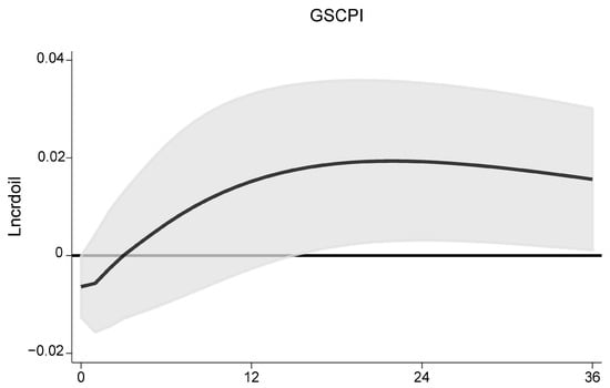
Figure 3.
IRF of crude oil prices to GSCP shock, to one standard deviation. Note: median (line); percentiles 10–90 (gray band).
Figure 4 shows the orthogonal IRFs of the other variables to a positive GSCP shock. A rise in the GSCP index will reduce investors’ confidence in financial markets while increasing the risk-free rate, which could be related to the high inflation in the US triggered by supply chain disruption [35]. The responses of both crude oil production and global industrial output to a GSCP shock are negative, showing a decrease in production and deceleration of economic activity; these results are consistent with the findings of Abel et al. [36]. Using information from regional business surveys, they demonstrate that a large share of businesses responded to disruptions by increasing their selling prices and scaling back their operations; outlooks were particularly pessimistic among firms in the manufacturing, construction, retail, transportation and warehousing industries, which are important consumers of crude or refined oil. The NLR, which is a proxy for speculation, increases after a rise in GSCPI, but then declines over time. One possible explanation is that crude oil inventories increase after the supply chain disruption, as the crude oil cannot be delivered to the customers. Then, inventories start to decline because production decreases while customers use the existing inventories. Another explanation is that a rise in risk aversion can decrease net-long positions, as they require a higher risk premium to be taken in futures markets. According to the mainstream model for speculation on commodity markets [29,30], the speculator net-long positions in equilibrium are positively related to the optimal inventory level of producers and negatively related to the risk aversion of speculators; for example, the greater the net supply or inventories of physical commodities, the more short futures positions will be taken by the hedger, and the more long futures positions will be taken by the speculator to offset the hedger’s position. In Section 5.1, we confirm that crude oil inventories increase and then decline after a positive GSCP shock.
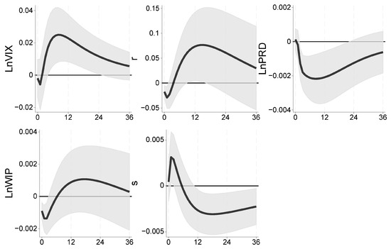
Figure 4.
IRFs of GSCPI shock to other variables, to one standard deviation. Note: median (line); percentiles 10–90 (gray band).
The orthogonal IRFs of crude oil prices to shocks to other variables, to one standard deviation, are presented in Figure 5. A rise in VIX leads to a reduction in crude oil prices, indicating the oil is a risky asset. A positive production shock will reduce oil prices, while a rise in global output will increase them; these results highlight the role of supply and demand, and are consistent with those of Baumeister and Hamilton (2019). More speculation or a higher net-long speculator ratio in the futures market can increase the price of oil, a notion widely accepted in both the market and academia [37,38]. However, the response to a risk-free-rate shock is insignificant, which is consistent with Kilian and Vega [39], who find that energy prices are predetermined with respect to monetary policy, as macroeconomic news tends not to immediately affect energy prices.
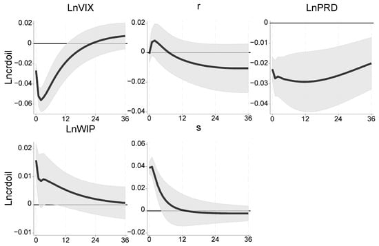
Figure 5.
IRFs of crude oil prices to shocks to other variables. Note: median (line); percentiles 10–90 (gray band).
From Figure 4 and Figure 5, we can conclude that although a positive GSCP shock can induce a rise in shipping costs and speculation and a decrease in production, which will increase crude oil prices, it can also lower the risk appetite of investors and the demand for crude oil, which will depress crude oil prices. This is because different channels may offset each other, and the final effect of a GSCP shock depends on which side dominates.
3.2. Comparison of Responses to GSCP Shocks in Different Periods
Supply chain disruptions have become a major challenge for the global economy since the onset of global trade tensions, especially the US–China trade war. After January 2018, global trade tensions started to escalate because of the unilateral trade policy of the United States; for example, on 22 January 2018, the US imposed 30% and 20% tariff rates on imports of solar panels and washing machines from China and elsewhere. Then, on 22 March 2018, President Trump explicitly asked the United States Trade Representative (USTR) to consider applying tariffs to Chinese goods with an ex ante value of USD 50–60 billion. Thus, the US and China began to engage in a trade war, and the tariff rates escalated on both sides. Though the tariff rates across many sectors ceased to rise until the inauguration of President Biden in 2020, the average tariff rates remained high and never decreased. Obviously, global supply and industrial chains can be disrupted by any instance of global trade tensions, not just by the US–China trade war; therefore, we set the start time of period 2 to January 2018, unlike other studies on the impact of the US–China trade war in January 2018 [40,41,42]. The global trade tensions not only disrupted the industry and supply chains, but also affected the economic outcomes in China, the US, and other countries through a spillover effect [40,41]. In addition, trade friction events can also trigger panic in financial markets [42,43]. Unlike in the US–China trade war, most supply chain disruptions during the COVID-19 pandemic were triggered by lockdowns or stringency policies in many countries. The lockdown policies not only increased crude oil transport and shipping costs, but also skewed the perspective of the global economy and led to risk-aversion behavior in investors [24,25]. Conversely, the global supply chain disruptions before 2018 were primarily related to natural disasters, transport-blocking events, or regional geopolitical conflicts; such events are infrequent and their effects short-term, so GSCP shocks during these periods would have a smaller impact on investor sentiment, production arrangement, and global economic activity, and thus a different impact on crude oil prices.
Figure 6 shows the IRFs of crude oil prices and other variables to GSCP shocks before and after the outbreak of global trade tensions (we refer to these periods as period 1 and period 2) (we do not present the IRFs of crude oil prices to shocks to other variables due to space limitations, but can provide them upon request). It is evident that the IRFs to a positive GSCP shock are quite different for the two periods. Specifically, in period 1, a positive GSCP shock increased crude oil prices immediately, and this effect lasted for some time, but prices decreased initially and then increased about 2 months later in period 2. We argue that this difference between the two periods can be explained by the other subplots in Figure 5, as the responses of the other variables to GSCP shocks also differ between the two periods. For example, a positive GSCP shock was accompanied by a reduction in risk appetite in period 1; one explanation may be that the Global Financial Crisis of 2007–2009 caused an upsurge in the VIX index and a drop in shipping costs; however, there was a rise in market panic during period 2. Similarly, the response of global industrial output was slightly positive in period 1, but in period 2, it was negative at first and then positive after 2–3 months; this indicates that the supply chain and industrial chain reorientation resulting from the China–US trade war, and the supply chain disruption caused by the stringency policies during the COVID-19 pandemic, decreased economic outcomes, which is supported by previous studies. It is clear that the response of crude oil production is negligible in period 1 and significantly negative in period 2, suggesting that crude oil producers cease production after a positive GSCP shock, as demand shrinks and inventories increase passively in a short time; this reduction in production is an important reason for the increment in crude oil prices after a few months in period 2. The negative impact of indirect channels is initially greater than the positive impact of direct channels, resulting in a decrement in crude oil prices after a positive GSCP shock in period 2.
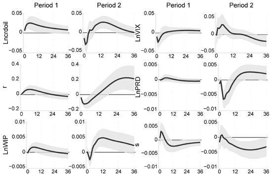
Figure 6.
Comparison of IRFs of crude oil prices and other variables to GSCP shocks in periods 1 and 2. Note: median (line); percentiles 10–90 (gray band).
In order to compare the contributions of GSCP shocks to oil price fluctuations in three sample periods, we decomposed oil price variances into seven components using the variance decomposition approach, and the results are shown in Table 3 (in order to save space, we only show the contributions of GSCP shocks in this paper, but the complete results can be provided upon request). Notably, the contributions of GSCP shocks are much smaller during period 1, especially in a short time (6 months). However, they increase dramatically during period 2, indicating that GSCP shocks play an important role in oil price fluctuations during this period; these results are consistent with the fact that global supply chain disruptions have become an important factor in the world economy and the turbulence of global financial markets.
Table 3.
Contributions of GSCP shocks to oil price fluctuations.
3.3. Comparison of Responses to GSCP Shocks with Different Commodities
We also investigated the responses of other commodity prices to GSCP shocks, and discuss whether their responses are heterogeneous across two periods. Specifically, we replaced the production (in logarithm, and season-adjusted), speculation, and real futures price (in logarithm) of a commodity for crude oil in Equation (2), and kept the other variables and restriction identifications unchanged. We selected gold, copper (COMEX), heating oil (NYMEX), soybean, corn, and wheat (CBOT), which are traded on the major commodity exchanges, for comparison, as these commodities include precious metals, industrial metals, energy, and agricultural products, and are also representative of commodity futures markets. Like for crude oil, we also used the real price of each commodity, which is deflated by the U.S. CPI index, and the data for futures prices were obtained from WIND Info. We calculated the speculation for each commodity using COT reports; in addition, we obtained the data for the production of global refined copper (primary + recycled) from ICSG and the data for the production of gold and agricultural products from WIND Info. As there was no data for the production of heating oil, we utilized data on crude oil production instead.
Figure 7 shows the IRFs of the prices of six commodities to GSCP shocks in three sample periods. It is found that the prices of all six commodities rise after the GSCP shock in period 1. In period 2, the responses of the prices tend to be insignificant (for agricultural products) or even negative (for heating oil) initially, and then become significantly positive about 4–5 months later in. However, the response of gold prices is initially significantly positive in period 2, which continues for some time. Therefore, though the IRFs of futures prices to GSCP shocks are heterogeneous across commodities, their responses (except for gold) are somewhat similar to that of crude oil.
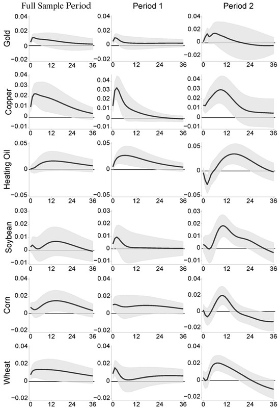
Figure 7.
IRFs of crude oil prices to GSCPI shocks, to one standard-deviation, during the full sample period and in periods 1 and 2. Note: median (line); percentiles 10–90 (gray band).
We argue that GSCP shocks have slight impacts on the other variables, except for speculation, in period 1. The responses of other common variables (such as VIX, global industrial output, and risk-free rate) and speculation to a positive GSCP shock for the selected commodities in the three periods are similar to those given in Figure 3 and Figure 5 but different from that of crude oil. The IRFs of production are also negligible for the selected commodities because the supply of these commodities is always stable or affected by other factors. For example, Stuermer [44] points out that the commodity supply is relatively stable in the short term, and agricultural production is influenced predominantly by agricultural technologies and seasonal factors [45] (in order to save space, the corresponding results are not presented here but will be made available on request). The low impact of GSCP shocks on these variables means that the direct channel (primarily the shipping cost channel) dominates and the effect of the indirect channel is negligible, thus generating similar IRFs of futures prices for all of the selected commodities (including crude oil). As most of the selected commodities, except for gold, are pro-cyclical, risky assets, the decrement in industrial output and increment in VIX triggered by a positive GSCP shock in period 2 also initially depress the prices of these commodities and partially offset the effect of the direct channel. While gold is regarded as a typical safe-haven asset and its price is insensitive to the global output growth, its price also increases after a GSCP shock in period 2. Figure 8 demonstrates that the IRFs of gold prices to the VIX index and global industrial output are quite different from those of the other commodities. It should be noted that copper mining and copper production processes occur in different locations, making copper prices more sensitive to maritime transportation costs. For example, the global distribution of copper mines is relatively concentrated, with mines primarily located in countries such as Chile, Peru, Australia, and the Democratic Republic of the Congo; however, copper smelting is concentrated in China, Japan, and the United States. Therefore, for copper, the indirect effect of a GSCP shock may be less severe than the direct effect, resulting in an initial price increment in period 2, although copper is also widely regarded as a pro-cyclical commodity.
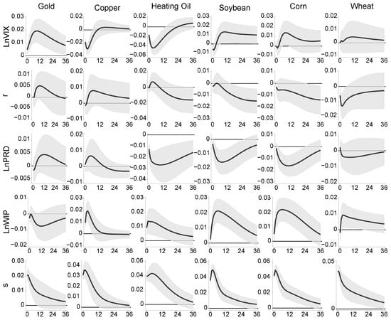
Figure 8.
IRFs of selected commodity prices to shocks to other variables in the whole sample period. Note: median (line); percentiles 10–90 (gray band). Like for crude oil, the results for periods 1 and 2 are similar, and we do not show the results here due to space limitations.
We also decomposed the other commodities into seven components and analyzed the degree to which GSCP shocks contributed to their price variations in the three sample periods. Table 4 shows the results. Similar to Table 3, the contributions of GSCP shocks increased considerably more for the six commodities in period 2 than in period 1, especially for copper and heating oil, which are commonly regarded as “pro-cyclical” commodities. These results also support the idea that supply chain disruptions became more important for commodity markets after the outbreak of global trade tensions in 2018.
Table 4.
Contributions of GSCP shocks to other commodities’ prices fluctuations.
4. Explanations for the Movement of Global Supply Chain Pressure
Theoretically, a GSCP shock can be triggered by various factors, such as natural disasters, the blockage of key waterways, the lockdown policy adopted during the COVID-19 pandemic, and even global trade tensions, which may force firms to adjust their global procurement strategies [46]. For example, there was a substantial rise in the GSCP index in 2011, attributable to two natural disasters (the Tohoku earthquake in Japan and a flood in Thailand), and it has increased again since the outbreak of global trade tensions in January 2018. In addition, the index soared to an unprecedented level after the outbreak of the COVID-19 pandemic. As market participants have different reactions to shocks under different circumstances, it is necessary to assess the reasons for the movement of the GSCP index and to provide further explanations for the heterogeneous impact of GSCP shocks between periods 1 and 2.
Combined with explanations of the components of the GSCP index, we divided the explanatory variables into four categories: (1) Natural disasters and the blockage of key waterway: In this study, we established four dummy variables to represent the Tohoku earthquake (), a flood in Thailand (), and the blockage of the Suez () and Panama canals (), respectively. The variables had a value of 1 during the event period and 0 otherwise. (2) Geopolitical risk: Political conflicts, including wars between countries, can disrupt the global supply chain by exacerbating the risk of transportation procedures and increase the cost of transporting commodities and manufacturing products. For example, the Russia–Ukraine war has reduced the supply of gas and crude oil from Russia to EU, and the export of grains from Russia and Ukraine, thus leading to global supply chain disruption. Following the methods used in the related literature, we utilized the logarithm of geopolitical risk index () constructed by Caldara and Iacoviello to proxy global geopolitical risk (The data were obtained from the personal website of Matteo Iacoviello (www.matteoiacoviello.com/gpr.htm, accessed on 16 May 2025)). It should be noted that the Al-Houthi movement in Yemen has been attacking ships in the Red Sea since November of 2023, resulting in a pause in voyages across the Red Sea by some of the world’s largest shipping companies, such as Maersk, Hapag-Lloyd, MSC, and CMA CGM, and a surge in shipping costs from Asia to Europe. Therefore, we established a dummy variable () to reflect the impact of this unique geopolitical event, which had a value of 1 after November of 2023 and 0 otherwise. (3) The lockdown policy during COVID-19. We utilized the logarithm of 1 plus the stringency index calculated by the Oxford Coronavirus Government Response Tracker project (for more information on the stringency index, see https://ourworldindata.org/metrics-explained-covid19-stringency-index, accessed on 16 May 2025) as a proxy for the strictness of globally government policies (). As the data for the stringency index spans only from January 2020 to December 2022, and the values of the data range from 0 to 100, we set the value of the stringency index to 0 for periods that did not fall within this date range. Though this is a simple method of handling the stringency issue for periods other than the COVID-19 pandemic, there were almost no lockdown policies around the world during these periods, and only a few countries imposed strict social distancing limitations in our sample period; for example, China restricted the population’s mobility in certain areas during the COVID-19 period. A higher stringency index score indicates a stricter lockdown policy and may lead to a higher GSCP index. (4) Global trade tensions. We established a dummy variable () with a value of 1 for the period after January 2018 and 0 otherwise, as global trade tensions started to rise after that time. In order to verify whether the change in tariff rates impacted the GSCP index, we also constructed an interaction term, (where is the average US tariff rate on Chinese exports). The data were obtained from the PIIE website (https://www.piie.com/research/piie-charts/2019/us-china-trade-war-tariffs-date-chart, accessed on 16 May 2025). In the trade war, China retaliated quickly after the US imposed a higher tariff rate on its imports, and the tariff rate imposed by China on exports from the US is approximately equivalent to the tariff rate imposed by the US. Therefore, we used the average US tariff rate on Chinese exports to reflect the degree of global trade tensions (primarily the US–China trade war) and used the interaction term as an alternative proxy for global trade tensions.
Finally, we established the following empirical model:
The regression results of Equation (4) are shown in Table 5, where columns (1) to (9) present the results of the univariate analysis, and the results of the multivariate analysis are presented in column (10). Among the four dummy variables for natural disasters and the blockage of key waterways, only the coefficient of is significantly positive, while the coefficients of and are insignificantly positive; this indicates that the blockage of the Suez canal had a significant impact on the global supply chain, while the impact of other factors in this category is negligible. The impact of geopolitical risk is statistically insignificant even though the coefficient of is positive; the explanation may lie in the fact that many global geopolitical events are unrelated to transportation costs or industrial reorientation. Similarly, the coefficient of is also insignificant.
Table 5.
The empirical results for the determination of GSCP index.
Contrary to the factors in the previous two categories, the impact of the stringency index during the COVID-19 pandemic is significantly positive, and the value of is high in column (6), reflecting the high explanation power of this variable regarding the movement of the GSCP index. In order to improve the robustness of the econometric results on the role of stringency policies, we confined our sample period to the COVID-19 pandemic and conducted a univariate analysis. The results are shown in column (11) of Table 5, and indicate that the stringency index caused movement of the GSCP index during the COVID-19 pandemic. Similarly, the coefficient of is also significantly positive, and the value of is also relatively large in column (7), suggesting that global trade tensions (especially the US–China trade war) originating from the protective trade policy put in place by the US caused not only a decline in international trade, but also global supply chain disruption and a rise in the GSCP index. Interestingly, the coefficient of the interaction term is also significant, with a higher value of in column (8) than in column (7). The results in column (10) confirm the findings of the univariate analysis. As the COVID-19 lockdown policy and global trade tensions have a significant and important influence on the evolution of the GSCP index, and have negative impacts on the growth of industrial output (the demand for crude oil) and market sentiment, they have an important impact on crude oil production and speculation on its futures markets. Therefore, the findings in Table 5 provide further explanation of the differences in the responses of crude oil prices and other variables to GSCP shocks.
5. Robustness Test
5.1. Replacing the Speculation Variable with the Inventory Variable
It is evident that futures prices have been affected by the speculative activity in futures markets, and the movement of speculation is also linked to the evolution of producers’ inventories in spot markets [29,30]. Therefore, we replaced the speculation variable () with the inventory level () (we obtained an estimate of global crude oil stocks, as in Baumeister and Hamilton [14] and Kilian and Murphy [47], by multiplying the US crude oil inventories by the ratio of OECD inventories of crude petroleum and petroleum products to US inventories of petroleum and petroleum products) in Equation (2), and the identifying restrictions were kept the same as before. The corresponding IRFs of crude oil prices to a positive GSCP shock in the whole sample period, and in periods 1 and 2, are shown in Figure 9 (due to space limitations, we only present the responses of crude oil prices and inventory to GSCP shocks; the other results are the same as in Figure 2, Figure 3 and Figure 4). It is obvious that the responses of crude oil prices in the three periods are similar to those in Figure 1 and Figure 4. In particular, the response of inventory to a GSCP shock is small in period 1, but significantly positive in period 2, indicating that producers tend to accumulate inventory after a GSCP shocks to stabilize their current production; however, production and inventory then begin to reduce, and the result is consistent with the response of production to a GSCP shock in Figure 5.
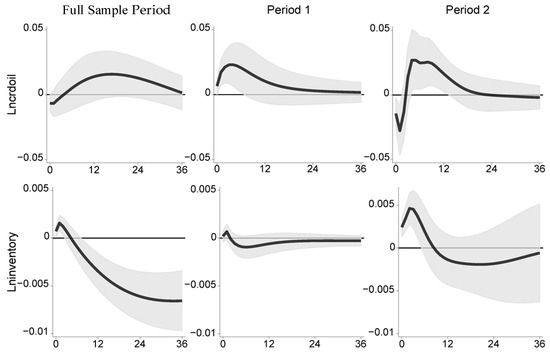
Figure 9.
IRFs of price and inventory of crude oil to a positive GSCP shock in the whole sample period, and in periods 1 and 2. Note: median (line); percentiles 10–90 (gray band).
5.2. Using Different Identifying Restrictions in the SVAR Model
This investigation was motivated by Basher et al. (2012), who claimed that there is possibility that global oil demand cannot respond to oil supply shocks within the same month; that is to say, oil supply shocks do not have immediate effects on oil demand. To analyze whether this change will have a significant impact on the previous results, we set the value of a54 in Equation (3) as 0 and re-estimated the SVAR model. The responses of crude oil prices for the three periods are shown in Figure 10, and these results are the same as those in Figure 3 and Figure 6.
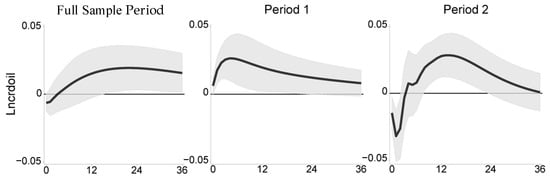
Figure 10.
IRFs of crude oil prices to a positive GSCP shock using new identifying restrictions. Note: median (line); percentiles 10–90 (gray band).
5.3. Splitting the Sample Period into Pre- and Post-Pandemic Periods
We split the whole sample period into two sub-periods in Section 3.2 based on the outbreak of global trade tensions, as we believe that both trade tensions and stringency policies during the COVID-19 pandemic would have similar impacts on the risk appetite of investors and the demand for crude oil, and thus on the production of crude oil. However, in reality, Figure 1 shows that the GSCP index rose dramatically from January of 2020 (we extend our thanks to an anonymous reviewer for pointing out this issue), indicating that the most important factor in the global supply chain disruptions is the lockdown policies triggered by the COVID-19 pandemic. Therefore, we divided the whole sample period into two sub-periods according to the outbreak of the COVID-19 pandemic, and the specific results of the SVAR model are presented in Figure 11. It is clear that the responses of crude oil prices to a GSCP shock in the pre- and post-pandemic periods are similar to the corresponding responses in Figure 6, Figure 9 and Figure 10, but different from the aforementioned ones; in addition, the initial response in the post-pandemic period is insignificant. One possible explanation is that the lockdown policies exerted more pressure on the cost of transporting crude oil compared with global trade tensions in period 2, causing the direct effect of GSCP shocks in the post-pandemic period to play a greater role than in the pre-pandemic period. As global trade tensions and the COVID-19 pandemic had similar effects on the risk appetite of investors and global demand for crude oil, and thus the global production of crude oil, and global trade tensions still disrupted the global supply chain even after the end of COVID-19 pandemic, it is reasonable to divide the whole sample period into two sub-periods as in Section 3.2.
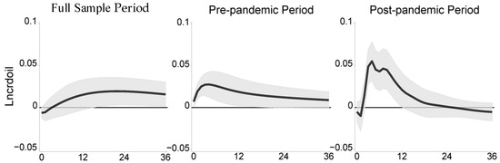
Figure 11.
IRFs of crude oil prices to a positive GSCP shock in the whole sample period, and in the pre- and post-pandemic periods. Note: median (line); percentiles 10–90 (gray band). The pre-pandemic period ranges from 1998M1 to 2019M12, and the post-pandemic period ranges from 2020M1 to 2024M6.
6. Conclusions
This study employs a structural VAR (SVAR) model to explore the effect of global supply chain pressures on crude oil prices. We draw the following conclusions. First, we found that a positive GSCP shock can impact prices through direct and indirect channels, which include demand, production, speculation in futures markets, and risk premium in financial markets. Second, after a positive GSCP shock, crude oil prices rose immediately before the outbreak of global trade tensions in 2018; however, after 2018, they became depressed initially and then rebounded about 2 months later. This response heterogeneity is primarily related to differences in the key reasons for the movement of the GSCP index between the two periods. Therefore, the manner in which a GSCP shock affects the prices of commodities depends on the characteristics and source of the GSCP shock, which indicates that investors in the commodity market should scrutinize the key driving factors behind global supply chain disturbances. Our conclusions are somewhat different to those of previous studies on financial markets that focus on equity, cryptocurrency, or commodities [6,7,8,9,10,13], as we consider the characteristics of key drivers of the movement of the GSCP index; therefore, our study expands upon the current understanding of the effect of supply chain disruptions on commodity markets.
This study carries some implications for policymakers and investors. For policymakers, first, international cooperation is needed to alleviate global supply chain disruptions, especially anthropogenic disruptions such as global trade tensions and geopolitical conflicts, and to improve the resilience of supply chains to achieve broader sustainability goals; for example, investment in alternative routes (including Eurasian Continental Bridge) should be encouraged to address the blockage of key waterways such as the Suez Canal, and global trade agreements should be reached on important issues such as tariff rates and prices set by agricultural producers. Second, policymakers should establish a granular supply-chain stress-monitoring framework, prioritizing shock-origin differentiation to formulate targeted response strategies. For example, to address the post-2018 delayed-price-rebound phenomenon during trade tensions, authorities should refrain from implementing contractionary interventions during initial shock phases. Instead, they should maintain a 2-month policy observation window and preemptively deploy protocols for the strategic release of petroleum reserves to alleviate market volatility and ensure energy security. Third, enhancing cross-agency regulatory coordination in futures markets is imperative to the dynamic tracking of speculative positions and risk premium fluctuations, thereby mitigating the amplification of price overshooting risks through financial channels. For investors, moving beyond expectations of a unidimensional linear response toward GSCP shocks requires rigorous analysis of underlying drivers: based on historical patterns, geopolitical conflicts and supply-disruption shocks warrant tactical long positions, whereas global trade friction shocks (post-2018 paradigm) investors to be vigilant towards near-term downside risks while strategically positioning themselves for structural rebound opportunities approximately two months post-shock. Indicators futures market sentiment and financial conditions should be incorporated as critical parameters for dynamic hedge ratio adjustments.
This study has several limitations. First, although our model specifies indicators for factors influencing fluctuations in crude oil futures price, cross-market contagion effects from agricultural products, metals, and other commodities may also impact price dynamics. Current methodological constraints prevent quantitative isolation of these factors, potentially leading to underestimation of risk transmission through supply chain pressures across commodity portfolios. Second, constrained by data availability, the GSCP shock index employed serves as an aggregate quantitative measure and fails to differentiate between and examine the heterogeneous impacts stemming from distinct shock typologies—such as geopolitical conflicts, natural disasters, and armed conflicts. Third, we identify the non-linear features of the impact of GSCP shocks on crude oil prices by splitting the data, and while this is a convenient method, it is simple; therefore, more advanced econometric methods could be employed to explore the contingency of such impacts. These aspects merit further investigation in future research.
Author Contributions
Conceptualization, C.Y. and D.J.; Methodology, C.Y.; Software, D.J., Y.W. and Q.W.; Validation, C.Y. and D.J.; Formal analysis, C.Y. and D.J.; Resources, C.Y., Y.W. and Q.W.; Data curation, D.J., Y.W. and Q.W.; Writing—original draft preparation, C.Y. and D.J.; Writing—review and editing, C.Y. All authors have read and agreed to the published version of the manuscript.
Funding
This research received no external funding.
Conflicts of Interest
The authors declare no conflict of interest.
References
- Benigno, G.; Giovanni, J.; Groen, J.; Noble, A. A New Barometer of Global Supply Chain Pressures. Federal Reserve Bank of New York Liberty Street Economics, 4 January 2022. Available online: https://libertystreeteconomics.newyorkfed.org/2022/01/a-new-barometer-of-global-supply-chain-pressures/ (accessed on 16 May 2025).
- Akinci, O.; Benigno, G.; Heymann, R.; Giovanni, J.; Groen, J.; Lin, L.; Noble, A. The Global Supply Side of Inflationary Pressures. Federal Reserve Bank of New York, 28 January 2022. Available online: https://libertystreeteconomics.newyorkfed.org/2022/01/the-global-supply-side-of-inflationary-pressures/ (accessed on 16 May 2025).
- Nugroho, A.D.; Ma’ruf, M.I.; Nasir, M.A.; Fekete-Farkas, M.; Lakner, Z. Impact of global trade agreements on agricultural producer prices in Asian countries. Heliyon 2024, 10. Available online: https://www.cell.com/action/showPdf?pii=S2405-8440%2824%2900666-2 (accessed on 16 May 2025). [CrossRef] [PubMed]
- Diaz, E.M.; Cunado, J.; de Gracia, F.P. Commodity price shocks, supply chain disruptions and U.S. inflation. Financ. Res. Lett. 2023, 58, 104495. [Google Scholar] [CrossRef]
- Ascari, G.; Bonam, D.; Smadu, A. Global supply chain pressures, inflation, and implications for monetary policy. J. Int. Money Financ. 2024, 142, 103029. [Google Scholar] [CrossRef]
- Ginn, W. Global supply chain disruptions and financial conditions. Econ. Lett. 2024, 239, 111739. [Google Scholar] [CrossRef]
- Finck, D.; Tillman, P. The Macroeconomic Effects of Global Supply Chain Disruptions; Bank of Finland Institute for Emerging Economies BOFIT Discussion Papers; Bank of Finland Institute for Emerging Economies BOFIT: Helsinki, Finland, 2022; BOFIT Discussion Papers 14. [Google Scholar]
- Hu, G.; Gozgor, G.; Lu, Z.; Mahalik, M.K.; Pal, S. Determinants of renewable stock returns: The role of global supply chain pressure. Renew. Sustain. Energy Rev. 2024, 191, 114182. [Google Scholar] [CrossRef]
- Kong, F.; Gao, Z.; Camelia, O. Green bond in China: An effective hedge against global supply chain pressure? Energy Econ. 2023, 128, 107167. [Google Scholar] [CrossRef]
- Li, Z.Z.; Su, C.W.; Moldovan, N.C.; Umar, M. Energy consumption within policy uncertainty: Considering the climate and economic factors. Renew. Energy 2023, 208, 567–576. [Google Scholar] [CrossRef]
- Qin, M.; Su, C.W.; Pirtea, M.G.; Peculea, A.D. The essential role of Russian geopolitics: A fresh perception into the gold market. Resour. Policy 2023, 81, 103310. [Google Scholar] [CrossRef]
- Rajput, H.; Changotra, R.; Rajput, P.; Gautam, S.; Gollakota, A.R.K.; Arora, A.S. A shock like no other: Coronavirus rattles commodity markets. Environ. Dev. Sustain. 2021, 23, 6564–6575. [Google Scholar] [CrossRef]
- Gozgor, G.; Khalfaoui, R.; Yarovaya, L. Global supply chain pressure and commodity markets: Evidence from multiple wavelet and quantile connectedness analyses. Financ. Res. Lett. 2023, 54, 103791. [Google Scholar] [CrossRef]
- Baumeister, C.; Hamilton, J.D. Structural interpretation of vector autoregressions with incomplete identification: Revisiting the role of oil supply and demand shocks. Am. Econ. Rev. 2019, 109, 1873–1910. [Google Scholar] [CrossRef]
- Kilian, L.; Zhou, X. Oil prices, exchange rates and interest rates. J. Int. Money Financ. 2022, 126, 102679. [Google Scholar] [CrossRef]
- Robe, M.A.; Wallen, J. Fundamentals, derivatives market information and oil price volatility. J. Futures Mark. 2016, 36, 317–344. [Google Scholar] [CrossRef]
- Adrian, T.; Shin, H.S. Liquidity and leverage. J. Financ. Intermediation 2010, 19, 418–437. [Google Scholar] [CrossRef]
- Manera, M.; Nicolini, M.; Vignati, I. Modelling futures price volatility in energy markets: Is there a role for financial speculation? Energy Econ. 2016, 53, 220–229. [Google Scholar] [CrossRef]
- Sims, C.A. Macroeconomics and reality. Econometrica 1980, 48, 1–48. [Google Scholar] [CrossRef]
- Toda, H.Y.; Yamamoto, T. Statistical inference in vector autoregressions with possibly integrated processes. J. Econom. 1995, 66, 225–250. [Google Scholar] [CrossRef]
- Chen, H.; Liao, H.; Tang, B.J.; Wei, Y.M. Impacts of OPEC’s political risk on the international crude oil prices: An empirical analysis based on the SVAR models. Energy Econ. 2016, 57, 42–49. [Google Scholar] [CrossRef]
- Basher, S.A.; Haug, A.A.; Sadorsky, P. Oil price, exchange rates and emerging stock markets. Energy Econ. 2012, 34, 227–240. [Google Scholar] [CrossRef]
- Kilian, L. Not all oil price shocks are alike: Disentangling demand and supply shocks in the crude oil market. Am. Econ. Rev. 2009, 99, 1053–1069. [Google Scholar] [CrossRef]
- Li, J.; Ruan, X.; Zhang, J. The price of COVID-19-induced uncertainty in the options market. Econ. Lett. 2022, 211, 110265. [Google Scholar] [CrossRef]
- McKibbin, W.; Fernando, R. The global economic impacts of the COVID-19 pandemic. Econ. Model. 2023, 129, 106551. [Google Scholar] [CrossRef]
- Benk, S.; Gillman, M. Identifying money and inflation expectation shocks to real oil prices. Energy Econ. 2023, 126, 106878. [Google Scholar] [CrossRef]
- Bessembinder, H. Systematic risk, hedging pressure, and risk premiums in futures markets. Rev. Financ. Stud. 1992, 5, 637–667. [Google Scholar] [CrossRef]
- De Roon, F.A.; Nijman, T.E.; Veld, C. Hedging pressure effects in futures markets. J. Financ. 2000, 55, 1437–1456. [Google Scholar] [CrossRef]
- Acharya, V.V.; Lochstoer, L.A.; Ramadorai, T. Limits to arbitrage and hedging: Evidence from commodity markets. J. Financ. Econ. 2013, 109, 441–465. [Google Scholar] [CrossRef]
- Li, B. Speculation, risk aversion, and risk premiums in the crude oil market. J. Bank. Financ. 2018, 95, 64–81. [Google Scholar] [CrossRef]
- Etula, E. Broker-dealer risk appetite and commodity returns. J. Financ. Econom. 2013, 11, 486–521. [Google Scholar] [CrossRef]
- Sanders, D.R.; Irwin, S.H. The impact of index funds in commodity futures markets: A systems approach. J. Altern. Invest. 2011, 14, 40–49. [Google Scholar] [CrossRef]
- Cheng, I.H.; Xiong, W. The financialization of commodity markets. Annu. Rev. Financ. Econ. 2014, 6, 419–441. [Google Scholar] [CrossRef]
- Fernandez-Perez, A.; Fuertes, A.-M.; Gonzalez-Fernandez, M.; Miffre, J. Fear of hazards in commodity futures markets. J. Bank. Financ. 2020, 119, 105902. [Google Scholar] [CrossRef]
- Amiti, M.; Heise, S.; Wang, A. High Import Prices along the Global Supply Chain Feed Through to U.S. Domestic Prices. Federal Reserve Bank of New York Liberty Street Economics, 8 November 2021. Available online: https://libertystreeteconomics.newyorkfed.org/2021/11/high-import-prices-along-the-global-supply-chain-feed-through-to-u-s-domestic-prices/ (accessed on 16 May 2025).
- Abel, J.; Bram, J.; Deitz, R.; Lu, J. Severe Supply Disruptions Are Impeding Business Activity in the Region. Federal Reserve Bank of New York Liberty Street Economics, 21 October 2021. Available online: https://libertystreeteconomics.newyorkfed.org/2021/10/severe-supply-disruptions-are-impeding-business-activity-in-the-region/ (accessed on 16 May 2025).
- Tang, K.; Xiong, W. Index investment and the financialization of commodities. Financ. Anal. J. 2012, 68, 54–74. [Google Scholar] [CrossRef]
- Singleton, K. Investor flows and the 2008 boom/bust in oil prices. Manag. Sci. 2014, 60, 300–318. [Google Scholar] [CrossRef]
- Kilian, L.; Vega, C. Do energy prices respond to U.S. macroeconomic news? A test of the hypothesis of predetermined energy prices. Rev. Econ. Stat. 2011, 93, 660–671. [Google Scholar] [CrossRef]
- Amiti, M.; Redding, S.J.; Weinstein, D. The Impact of the 2018 Trade War on U.S. Prices and Welfare; NBER Working Paper; National Bureau of Economic Re: Cambridge, MA, USA, 2019; No. 25672. [Google Scholar]
- Bown, C.P. The US-China Trade War and Phase One Agreement; Peterson Institute for International Economics Working Paper; Peterson Institute for International Economics: Washington, DC, USA, 2021; Working Paper 21-29. [Google Scholar]
- Carlomagno, G.; Albagli, E. Trade wars and asset prices. J. Int. Money Financ. 2022, 124, 102631. [Google Scholar] [CrossRef]
- Burggraf, T.; Fendel, R.; Huynh, T.L.D. Political news and stock prices: Evidence from Trump’s trade war. Appl. Econ. Lett. 2020, 27, 1485–1488. [Google Scholar] [CrossRef]
- Stuermer, M. 150 years of boom and bust: What drives mineral commodity prices? Macroecon. Dyn. 2018, 22, 702–717. [Google Scholar] [CrossRef]
- Sørensen, C. Modeling seasonality in agricultural commodity futures. J. Futures Mark. 2002, 22, 393–426. [Google Scholar] [CrossRef]
- Nugroho, A.D.; Masyhuri, M. Comparing the impacts of economic uncertainty, climate change, COVID-19, and the Russia-Ukraine conflict: Which is the most dangerous for EU27 food prices? Stud. Agric. Econ. 2024, 126, 18–25. [Google Scholar] [CrossRef]
- Kilian, L.; Murphy, D. Why Agnostic Sign Restrictions Are Not Enough: Understanding the Dynamics of Oil Market VAR Models. J. Eur. Econ. Assoc. 2012, 10, 1166–1188. [Google Scholar] [CrossRef]
Disclaimer/Publisher’s Note: The statements, opinions and data contained in all publications are solely those of the individual author(s) and contributor(s) and not of MDPI and/or the editor(s). MDPI and/or the editor(s) disclaim responsibility for any injury to people or property resulting from any ideas, methods, instructions or products referred to in the content. |
© 2025 by the authors. Licensee MDPI, Basel, Switzerland. This article is an open access article distributed under the terms and conditions of the Creative Commons Attribution (CC BY) license (https://creativecommons.org/licenses/by/4.0/).