Article

Application of a Modeling Framework to Mitigate Ozone Pollution in Changzhou, Yangtze River Delta Region

1
School of Environmental and Chemical Engineering, Shanghai University, Shanghai 200444, China
2
Chinese Academy of Environmental Planning, Beijing 100012, China
*
Authors to whom correspondence should be addressed.
These authors contributed equally to this study.
Sustainability 2025, 17(16), 7202; https://doi.org/10.3390/su17167202
Submission received: 2 July 2025 / Revised: 3 August 2025 / Accepted: 5 August 2025 / Published: 8 August 2025
(This article belongs to the Section Pollution Prevention, Mitigation and Sustainability)

Abstract

Ozone pollution in densely populated urban regions poses a great threat to public health, due to the intensive anthropogenic emissions of ozone precursors and is further aggravated by global warming and the urban heat island phenomenon. Air quality models have been utilized to formulate and evaluate air pollution control strategies. This study presents a comprehensive modeling assessment of ozone mitigation strategies during an ozone pollution episode in Changzhou, an industrial city in the Yangtze River Delta region. Utilizing the Community Multiscale Air Quality Modeling System (CMAQ), we quantified the contribution of ozone from different emission sectors and counties within Changzhou using the integrated source apportionment method (ISAM). During the pollution period, local emissions within Changzhou account for an average of 41.5% of MDA8 ozone, with particularly notable contributions from Jingkai (11.2%), Wujin (9.5%), and Liyang (7.8%). Upon these findings, we evaluated three sets of emission reduction scenarios: uniform, sector-specific, and county-specific reductions. Results show that industry and transportation are responsible for over 20% of ozone concentrations, and targeted reductions in these sources yielded the most significant decreases in ozone levels. Notably, reducing industrial emissions alone decreased ozone concentrations by 3.2 μg m−3 during the pollution episode. County-specific reductions revealed the importance of targeted strategies, with certain counties showing more pronounced responses to emission controls. On a daily basis, emission reductions in Xinbei contributed to a maximum ozone decrease of 4.4 μg m−3. This study provides valuable insights into the efficacy of different mitigation measures in Changzhou and offers a practical and useful framework for policymakers to implement strategies while addressing the complexities of urban air quality management.

1. Introduction

Ground-level ozone (O3) pollution in densely populated urban areas presents a great threat to public health [1,2,3,4], particularly affecting the growing elderly population that is more vulnerable to the adverse impacts of ozone exposure [5,6]. Driven by global warming, rising atmospheric temperatures typically enhance ozone formation [7,8]. Moreover, the urban heat island effect introduced by urbanization can indirectly aggravate ozone pollution in urban areas by altering local meteorological conditions [9,10,11]. These climate–urbanization feedback loops create complex sustainability challenges requiring integrated mitigation approaches. Over the past decade, the fine particulate matter (PM2.5) concentrations in China have notably declined at an average rate of 1.45 μg·m−3 per year from 2013 to 2022 [12]. In contrast, O3 concentrations have exhibited considerable fluctuations [13,14,15]. According to the China Blue Book of Atmospheric Ozone Pollution Prevention and Control [16], ozone levels in China from 2015 to 2022 initially exhibited a trend in fluctuating increase, followed by a phase of sustained high variability.
Three-dimensional air quality models, which simulate the physical and chemical processes of air pollution, have been extensively used in air quality management and planning [17,18,19,20]. For example, these models provide a technical foundation for the development of State Implementation Plans (SIPs) by offering data-driven insights into air quality trends, pollutant behavior, and the effectiveness of control measures [21,22]. Cheng et al. [17] integrate emissions, atmospheric, and health models to discuss how a synergistic strategy for air pollution control and carbon neutrality in China could prevent millions of premature deaths annually by 2060. In addition to formulating long-term control policies, air quality models also facilitate the evaluation of short-term control strategies aimed at mitigating peak pollution during heavy pollution periods [23,24]. For instance, Wang et al. [23] proposed a framework for the Joint Regional Prevention and Control (RJPC) program to eliminate a heavy PM2.5 pollution episode within the Fenhe Plain.
Numerous studies have focused on exploring effective strategies to alleviate ozone pollution across different regions in China. Zhang et al. [25] integrated ground-based measurements with model simulations to analyze changes in ozone formation sensitivity during a persistent pollution episode in Northeast China and explore its implications for developing effective ozone control strategies. Wang et al. [26] evaluated the ozone reduction potential in the Pearl River Delta region through O3-NOx-VOC sensitivity diagnosis and source apportionment. Results indicated that reducing precursor emissions in Dongguan contributes to improved air quality in the downwind area of Shenzhen. Tian et al. [27] quantified the contributions of cross-emission sources (between urban areas and sectors) to ozone concentrations and implemented targeted controls on anthropogenic emissions in the Central Plains urban agglomeration. Li et al. [28] simulated the response of ozone pollution in Lanzhou to precursor emissions and designed 11 emission control scenarios. Results show that a 10% reduction in NOx combined with a 20% reduction in total VOCs would lead to a decrease in ozone concentrations by up to 13% in urban Lanzhou and 16% in the western suburbs. However, despite these advances, there remains a critical gap: the absence of a unified framework that integrates source apportionment, scenario analysis, and policy evaluation to deliver actionable guidance for local policymakers.
This study addresses this gap by developing and applying a comprehensive modeling framework to evaluate ozone mitigation strategies. Using Changzhou—a typical industrial city in the Yangtze River Delta (YRD) region—as a case study, we demonstrate the framework’s practical utility and effectiveness. Changzhou, with its 5.4 million permanent residents and 1.7 million registered vehicles [29], serves as an important modern manufacturing hub characterized by a robust industrial base and diversified industries [30]. Developing effective ozone control strategies here is crucial for sustaining economic activity while safeguarding population health. In recent years, maximum daily 8 h average (MDA8) O3 concentrations in Changzhou have followed an upward trend, with the highest ozone levels and exceedance days (MDA8 O3 > 160 μg·m−3) occurring during summer months (June, July, and August). For instance, in June 2022, ozone concentrations exceeded the national standard (MDA8 O3 = 160 μg·m−3) on 43% of days, peaking at 248.9 μg·m−3, posing a severe public health risk. Previous studies have explored the mechanisms of ozone formation in Changzhou [31,32,33], revealing insights such as the shift in ozone generation mechanisms during the 2020 COVID-19 lockdown [32] and the influence of local chemical reactions and Lake Tai’s lake–land breeze on near-surface O3 levels [31]. Nevertheless, the previous studies have not provided a systematic analysis of ozone contributions from different sectors and regions within Changzhou, and there has been a lack of comprehensive evaluation of various mitigation strategies tailored to the city of Changzhou.
This study employs the widely recognized Community Multiscale Air Quality Modeling System (CMAQ) to present a comprehensive modeling framework for evaluating mitigation strategies during a severe ozone pollution episode in Changzhou. Using CMAQ’s integrated source apportionment method (ISAM), we quantify ozone contributions from different emission sectors and counties within Changzhou. Based on these findings, we develop multiple emission reduction scenarios, including uniform, sector-specific, and county-specific reductions, and evaluate their effectiveness in lowering ozone concentrations. Our sector- and county-specific reduction scenarios identify pathways to maximize ozone reduction, supporting resource-efficient sustainability planning. Our study provides valuable insights into the efficacy of different ozone mitigation measures during ozone pollution episodes in Changzhou and also offers a practical and useful framework for policymakers to implement strategies that protect public health while addressing the complexities of urban air quality management.

2. Materials and Methods

2.1. Methodological Framework

As shown in Figure 1, a framework is proposed for designing the optimal emission reduction strategies to mitigate O3 pollution in the target city. The process starts with the simulation of a base case scenario utilizing meteorology and air quality models. Observations of meteorological variables and O3 are employed to assess model performance. Subsequently, ozone source apportionment techniques are applied to quantify ozone contributions from diverse aspects, such as regional transport and surrounding cities, inter-county contributions within the target city, and emissions from various local source categories. Based on these source apportionment outcomes, a range of emission reduction scenarios are explored using the brute-force method. These scenarios encompass different NOx and VOC reduction ratios, county-specific emission reductions, and sector-specific emission reductions. The effectiveness of these scenarios in reducing O3 concentrations is evaluated to pinpoint a tailored ozone mitigation strategy for the target city.

2.2. Modeling Configuration

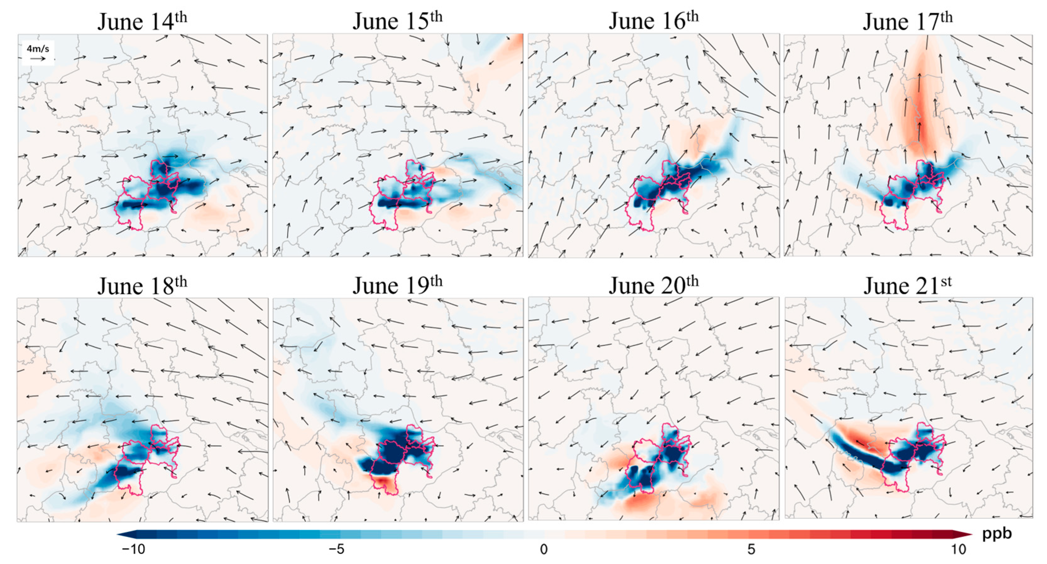
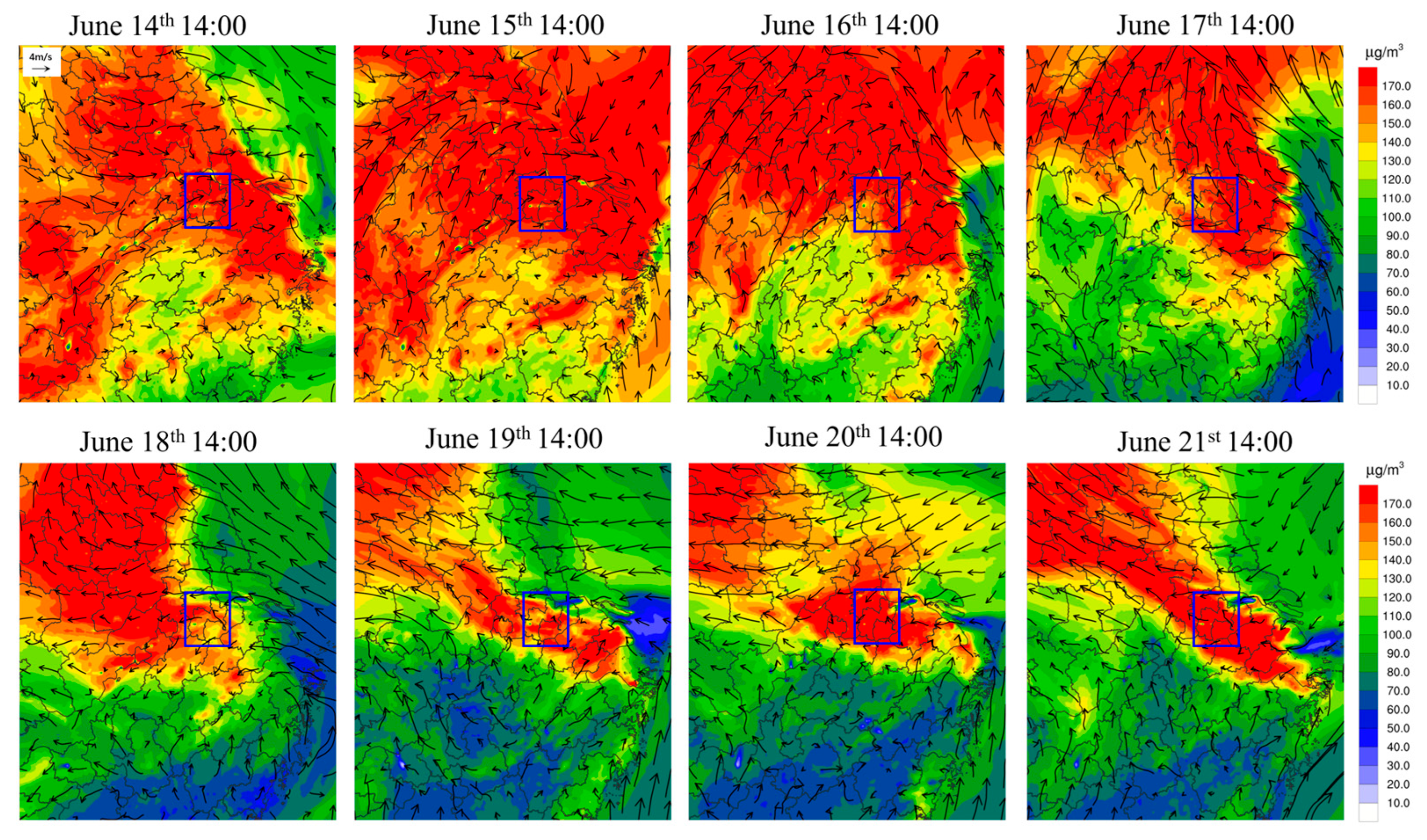
In this study, the Weather Research and Forecasting (WRF) model (version 4.0, https://www.mmm.ucar.edu/models, accessed on 11 November 2024) in conjunction with CMAQ version 5.3.2 [34] was used. The WRF and CMAQ configurations employed in this study were consistent with our previous studies [35], which are shown in Table A8. The modeling domain consists of three nested Lambert projection grids (Figure 2a) with spatial resolutions of 36 km, 12 km, and 4 km. Changzhou is located within the innermost grid, which encompasses the entire YRD region, including Anhui, Jiangsu, Zhejiang, and Shanghai. Boundary conditions for D01 were obtained from the default CMAQ profile, whereas those for D02 and D03 were derived from the outputs of their corresponding upper-level simulation domains. We employed the Carbon Bond mechanism (CB06) along with the AERO7 module to simulate gas-phase chemistry and aerosol formation. For anthropogenic emissions, we utilized the Multi-Resolution Emission Inventory of China (MEIC) developed by Tsinghua University (http://meicmodel.org, accessed on 11 November 2024), except in the YRD region, where anthropogenic emissions were consistent with those used in our prior studies [36,37]. The YRD emission inventory included emissions from power plants, industrial boilers and kilns, industrial processes, transportation, solvent use, oil and gas storage, residential, agriculture, dust, and biomass burning. Annual total emissions were allocated into hourly emissions with a spatial resolution of 4 km using the Sparse Matrix Operator Kernel Emissions (SMOKE) processing system [38]. Biogenic VOC emissions were calculated using the Model of Emissions of Gases and Aerosols from Nature (MEGAN version 3.2; https://bai.ess.uci.edu/megan, accessed on 1 November 2024). The specific ozone pollution episode selected for simulation spanned from 14 to 21 June 2022. During this 8-day period, the average MDA8 O3 concentrations reached 202.3 μg·m−3 with a peak concentration of 248.9 μg·m−3 observed on 18 June. The winds in Changzhou shifted from easterly to northerly during the first four days and then transitioned to persistent easterly winds starting from 18 June (Figure A17). The model was initialized with a five-day spin-up period to reduce the influence of initial conditions.
The ISAM module in the CMAQ model was applied to quantify the sectoral and county ozone contributions in Changzhou. For sectoral contributions, we identified six categories of emission sources: transportation, industrial processing, industrial boilers and kilns, power plants, natural emissions, and other sources (including biomass burning, residential emissions, solvent usage, oil and gas storage, dust, and shipping activities). In terms of county-level contributions, we quantified ozone contribution from each of the seven counties within Changzhou (Figure 2c): Jintan (JT), Xinbei (XB), Tianning (TN), Wujin (WJ), Jingkai (JK), Liyang (LY), and Zhonglou (ZL). For each county, the simulated ozone concentrations at the national monitoring station (if not available, the provincial monitoring station was used) were extracted and averaged to represent the county-level ozone concentrations.

2.3. Ozone Mitigation Scenarios

Although the ISAM results provided valuable information on ozone source contribution in Changzhou, the tagging-based method is not suitable for supporting air quality planning of non-linear species, like O3 [39,40]. To support air quality planning, three sets of ozone mitigation scenarios were developed to investigate their efficacy in reducing ozone levels using the brute-force method. These scenarios were categorized as “uniform emission reduction”, “sector-specific reduction”, and “county-specific reduction” (Table 1). In the “uniform emission reduction” scenarios, a consistent reduction ratio was applied across all emission sectors and counties within Changzhou. Various combinations of reduction ratios (20%, 40%, 60%) were tested for anthropogenic AVOC (AVOC) and anthropogenic NOx (ANOx), both separately and simultaneously, leading to a total of nine simulations conducted. In the “sector-specific reduction” scenarios, the emission reduction ratio was applied to one sector at a time while keeping other sectors unchanged (a total of five simulations). Similarly, in the “county-specific reduction” scenarios, the emission reduction ratio was applied to one county at a time, with emissions from other counties remaining unchanged (a total of seven simulations). Building upon the results from the “uniform emission reduction” scenarios, a 40% reduction ratio was exclusively applied to AVOC in both the sector-specific and county-specific scenarios. For emissions outside of Changzhou, we assumed a 20% emission reduction in NOx and AVOC to reflect the emission reduction efforts at the regional level.

2.4. Model Performance Evaluation

The model performance of baseline simulation (i.e., with no emission reductions) was evaluated by comparing simulated meteorological variables and ozone concentrations to observations. Several statistical metrics were used for model performance evaluation, including mean bias (MB), normalized mean bias (NMB), correlation coefficient (R), and index of agreement (IOA) (see Table A5 for detailed formulae). Hourly observed O3 concentration was obtained from the Ecological Environment Data Platform (https://quotsoft.net/air, accessed on 1 November 2024). Meteorological variables, including 2 m temperature (T), relative humidity (RH), and 10 m wind speed (WS) and wind direction, were from the National Meteorological Information Center (http://data.cma.cn/, accessed on 1 November 2024).
Simulated meteorological parameters were compared with observations in the YRD region (Table A6). Overall, the WRF model effectively captured the observed variations in T, WS, and RH in Changzhou. WS was slightly overestimated with an MB of 0.4 m/s and RH was underestimated with an NMB of −3.6%. Based on the results of the four provincial capital cities (Shanghai, Hangzhou, Nanjing, and Hefei), the simulated T and RH showed a strong correlation with the observed data, with R exceeding 0.8. WS was generally overestimated, with an MB ranging from 0.1 to ~0.4 m/s. However, RH tended to be underestimated with an NMB ranging from −14% to −8%. The overestimated wind speeds could lead to underestimated O3 concentrations due to the dispersion of O3 precursors and enhanced horizontal and vertical mixing of the atmosphere [41]. On the other hand, underestimated humidity could somehow offset the O3 underestimation as a negative correlation was usually found between humidity and O3 [42,43].
The validation of simulated O3 concentration is shown in Figure 3 and Table A7. In general, the CMAQ model was able to capture both the spatial and temporal variations in observed O3. During the selected pollution period (Figure 3b), the model showed an NMB of −1.0% and a spatial correlation coefficient of 0.9. Ozone underestimation was observed in northern and central Jiangsu, with MB ranging from 4.2 to ~27.0 µg·m−3. Furthermore, we compared the hourly O3 simulated concentrations for Changzhou and four provincial capitals in the YRD region (Figure 3c). During June 2022, R values ranged from 0.6 to 0.7 for these five cities. During the pollution period, the observed MDA8 O3 concentration in YRD region was 149.5 µg·m−3, whereas the simulated concentration was 147.5 µg·m−3. In summary, these results indicated acceptable model performance of the WRF and CMAQ model for further assessment of the efficacy of different emission reduction scenarios.

3. Results

3.1. Ozone Source Apportionment Based on CMAQ-ISAM

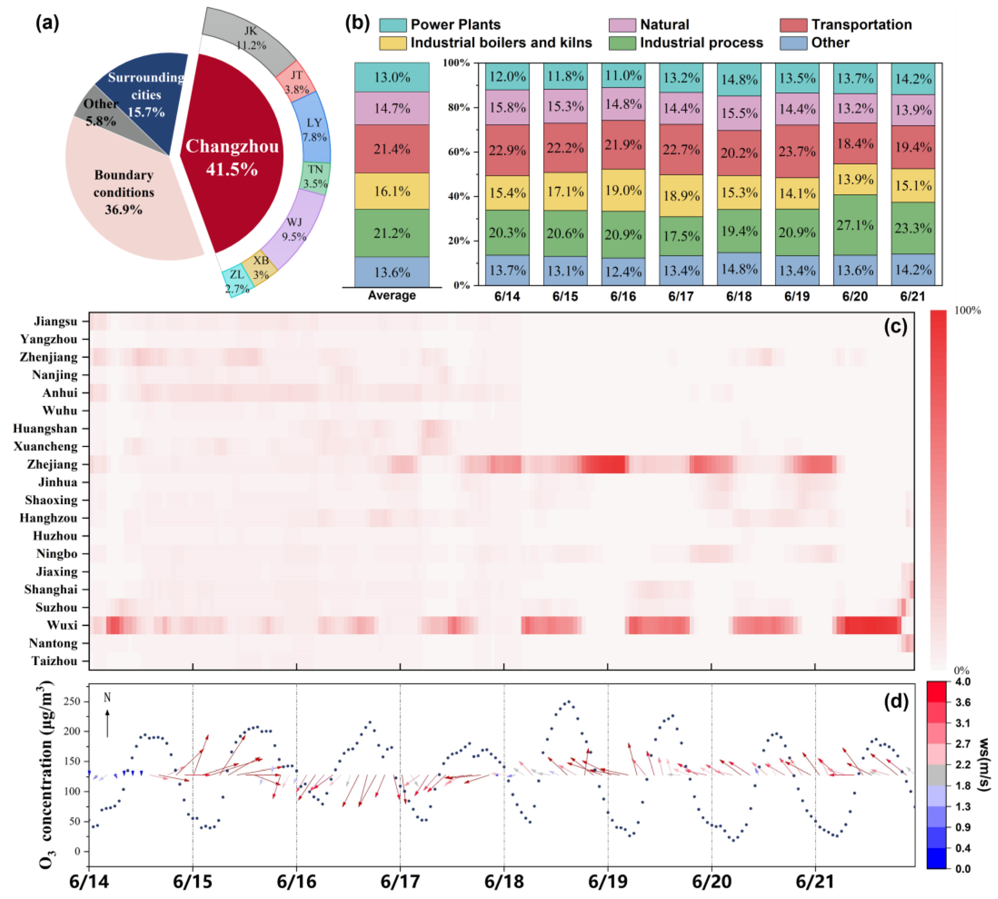
The regional and sectoral contributions of MDA8 during the selected pollution episode are shown in Figure 4. Local emission sources within Changzhou accounted for an average of 41.5% of MDA8 ozone, which was slightly higher than the contribution from boundary conditions (36.9%). On a daily basis, local sources could contribute as much as 75% (on 21 June). On a county-level (Figure 4a), the three counties with the highest contributions during the pollution episode were JK (11.2%), WJ (9.5%), and LY (7.8%), collectively accounting for ~28.5% of the total ozone contribution. The remaining counties (ZL, XB, TN, and JT) each contributed less than 5%, underscoring the spatial heterogeneity in emission impacts.
The average contributions from neighboring cities during the ozone episode amounted to 15.7%, and the relative importance of these surrounding cities varied primarily in response to changes in wind direction, with Wuxi (7.3%) exhibiting the highest contributions to ozone levels in Changzhou on average (Figure 4c,d). Compared to the monthly averaged results (Figure A2), the contributions from local sources during the pollution episode were considerably higher, underscoring the need for effective management of local emission sources. Among the various emissions within Changzhou (Figure 4b), industrial processes and transportation were responsible for over 20% of ozone concentrations, followed by emissions from industrial boilers and kilns (16.1%), biogenic sources (14.7%), and power plants (13.6%).
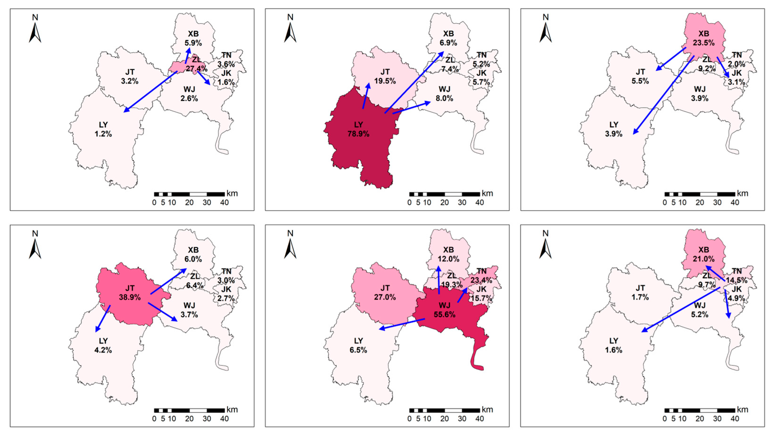
We further examined the inter-county contributions to ozone levels within Changzhou (Figure 5a). We designated each of the seven counties as a receptor and calculated the relative ozone contributions from all other counties. Additionally, each county was treated as a source region to quantify its ozone contributions to the other counties. Taking JK as an example, Figure 5b shows the relative ozone contributions from JK and other counties to the ozone levels in JK, with the total contributions aggregating to 100%. Local emissions within JK were predominant in ozone formation, contributing up to 66.1%. WJ, located upwind from JK, exhibited the highest contribution (15.7%) among the other counties, while contributions from other districts remained below 10%. Figure 5c further illustrates the ozone contribution from sources within JK to receptors in other counties. Emissions from JK primarily impacted TN, with a contribution of 48.3%, as it was directly downwind. JK’s contributions to WJ, ZL, and XB ranged from 20% to 30%. Overall, ozone levels in ZL and XB reflected a combination of local sources and contributions from neighboring counties, whereas WJ and JK not only exhibited the highest ozone concentrations but also contributed significantly to the ozone levels in other districts (Figure A3 and Figure A4). Notably, TN was particularly vulnerable to ozone transported from adjacent counties. The uneven source–receptor ozone contributions among different counties underscored the necessity for targeted county-specific emission reduction strategies in order to achieve the most cost-effective mitigation of ozone levels for the city of Changzhou.

3.2. Effectiveness Assessment of Different Mitigation Strategies

3.2.1. Uniform Emission Reductions

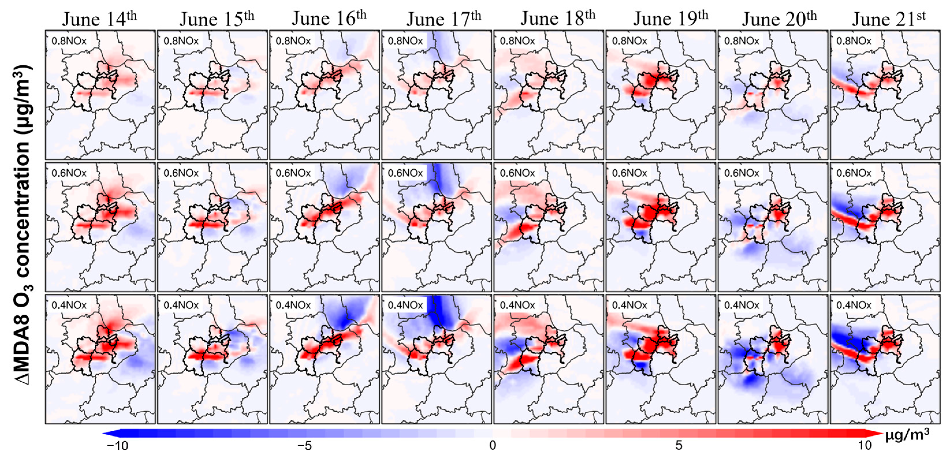
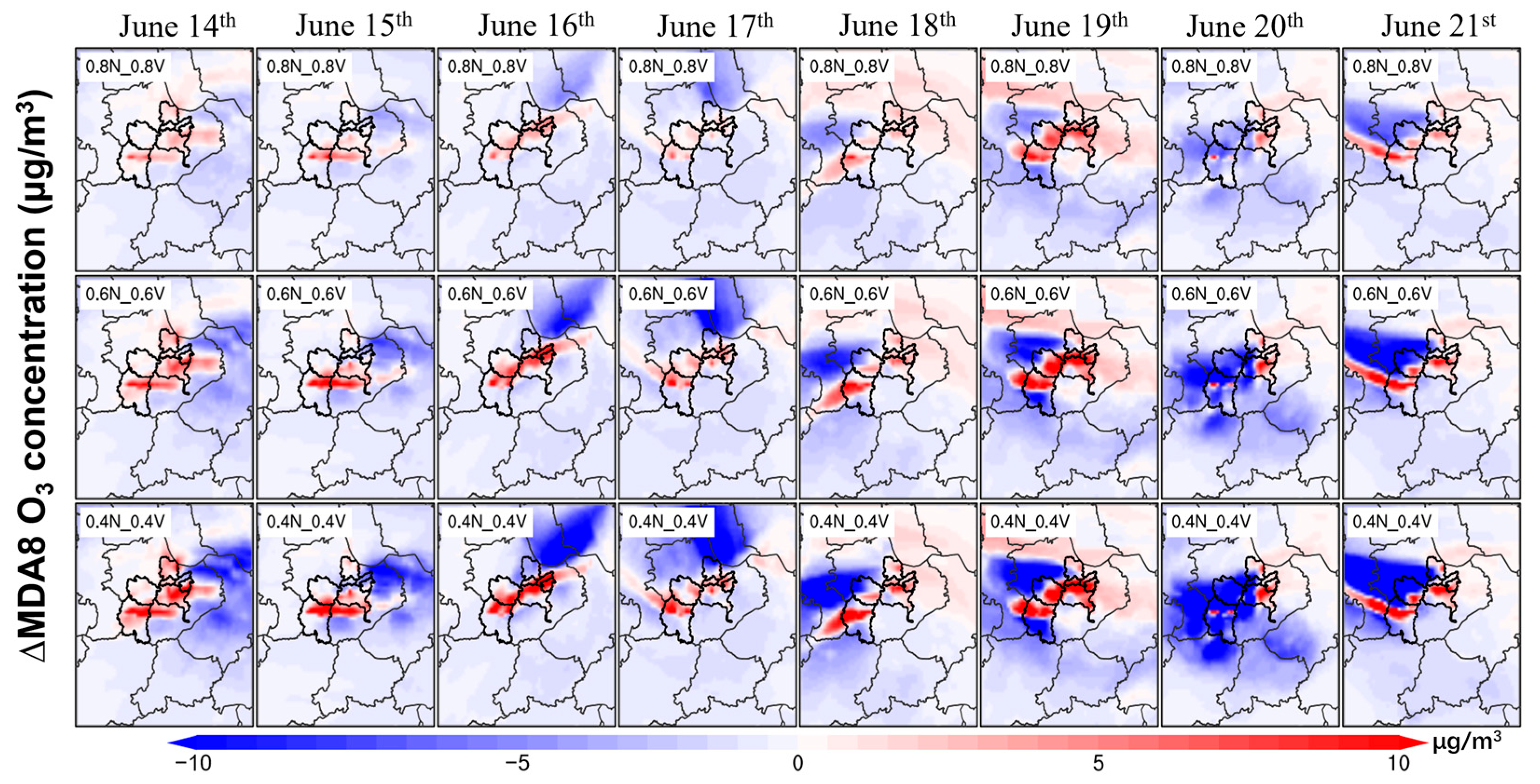
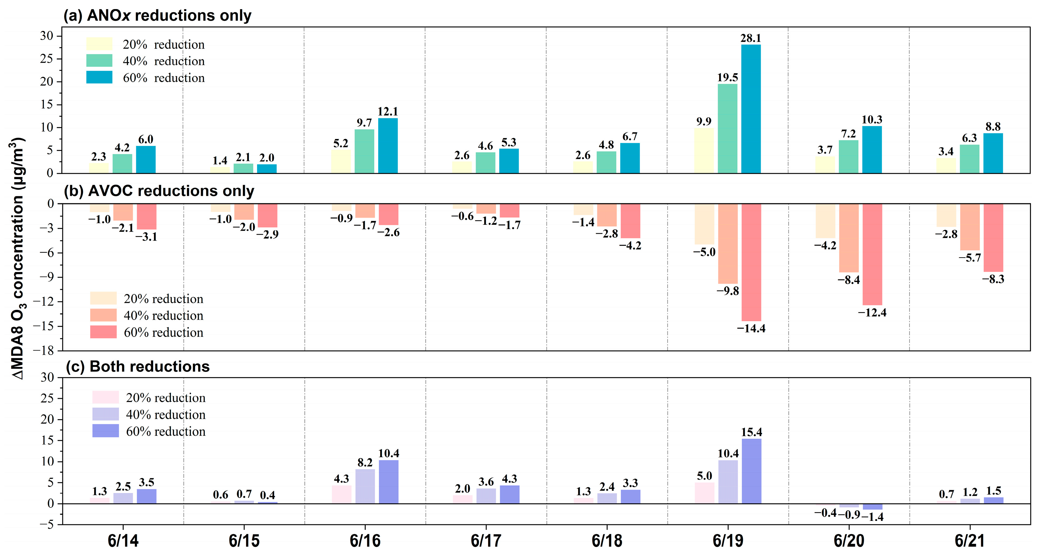
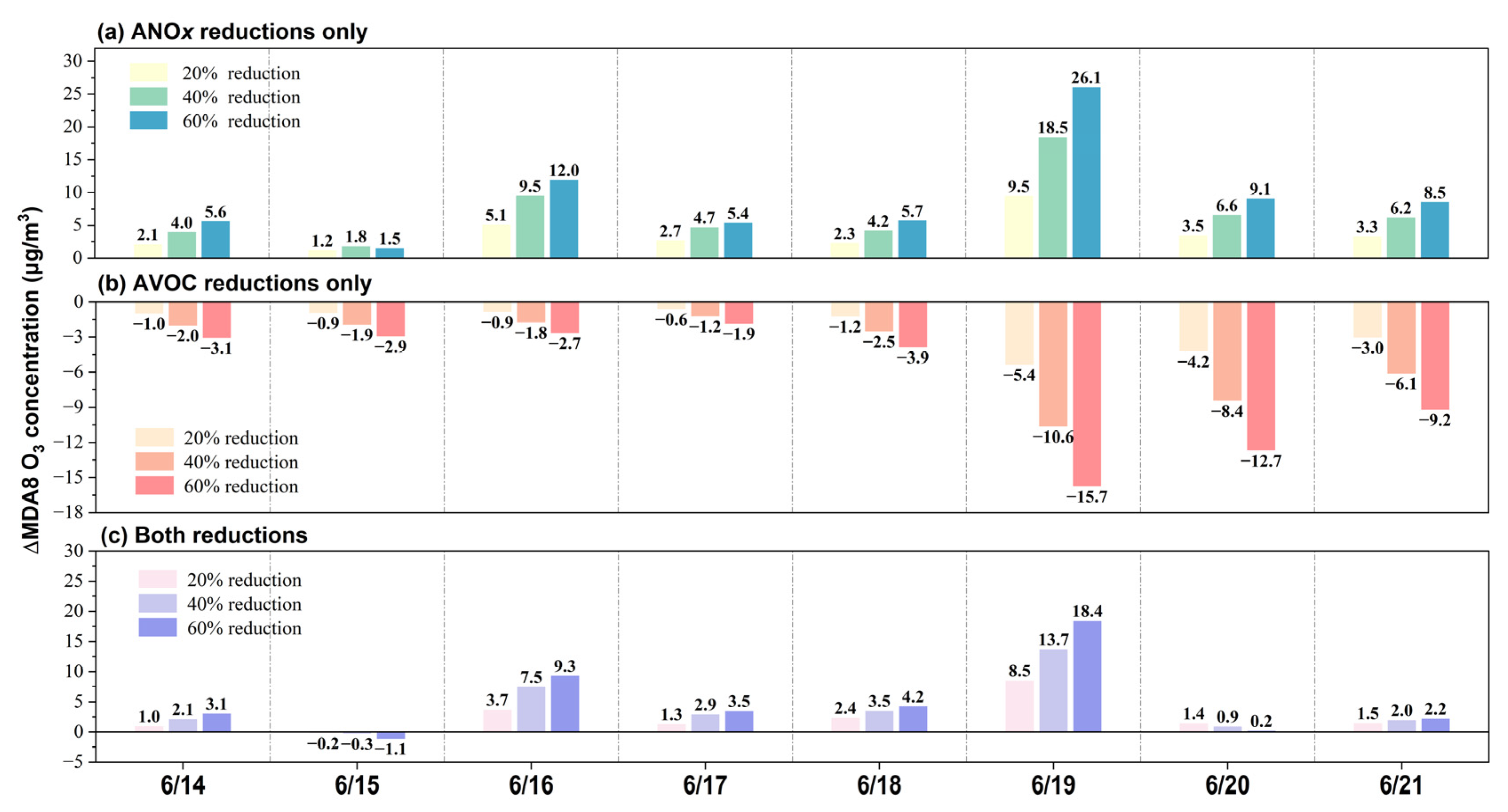
The uniform emission reduction scenario applied a consistent reduction ratio (20%, 40%, and 60%) to both ANOx and AVOC emissions across Changzhou. As illustrated by Figure 6, the reduction in ANOx emissions alone resulted in a notable rebound effect on ozone concentrations. For instance, a 20% reduction in ANOx emissions during the pollution period led to an average increase of 3.7 μg·m−3 in the MDA8 O3 concentrations in Changzhou, with WJ experiencing the largest increase of 5.7 μg·m−3. This nonlinear response of ozone concentration aligned with the CMAQ-DDM results (Figure A5 and Figure A6), which indicated a negative sensitivity of O3 to ANOx emissions, a trend that intensified with further reductions in ANOx reductions (Figure A7). On the other hand, when AVOC emissions were reduced independently, a clear downward trend in the average MDA8 ozone concentrations was observed (Figure 7 and Figure A8). Specifically, a 20% reduction in AVOC emissions resulted in a decrease of 2.2 μg·m−3 in ozone levels, with JT District showing the most pronounced decline. In scenarios where both ANOx and AVOC emissions were concurrently reduced, the opposing effects of these reductions yielded a modest increase in ozone concentrations across all counties (Figure A9), with the exception of LY. Notably, LY exhibited the smallest response in ozone levels to changes in emissions, attributed to its position upwind from Changzhou, which minimized the influence of emissions from other counties (1.2% to 6.5%, as shown in Figure 5a). Furthermore, LY was unique in that it experienced reductions in ozone when ANOx and AVOC were simultaneously reduced. These findings are consistent with previous studies showing that the summertime ozone formation in Changzhou was predominantly controlled by VOC [44,45,46], necessitating an AVOC to ANOx reduction ratio greater than one to effectively mitigate ozone levels [47,48].

3.2.2. Sector-Specific Emission Reduction

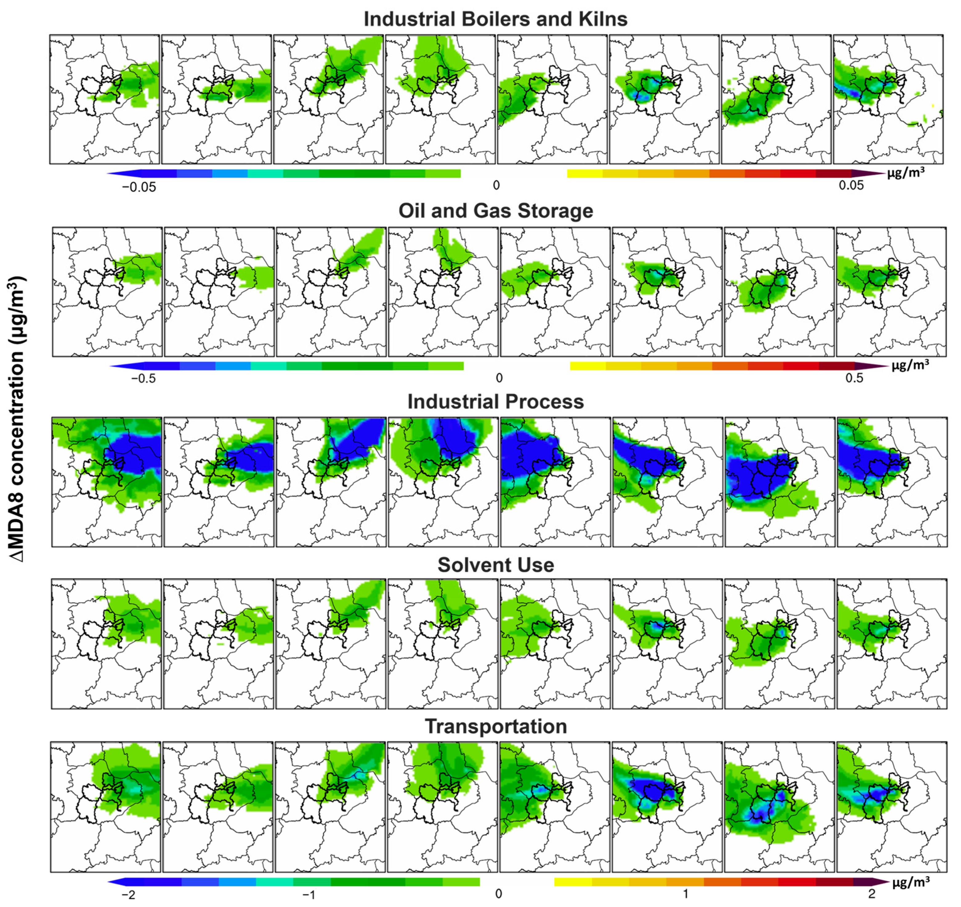
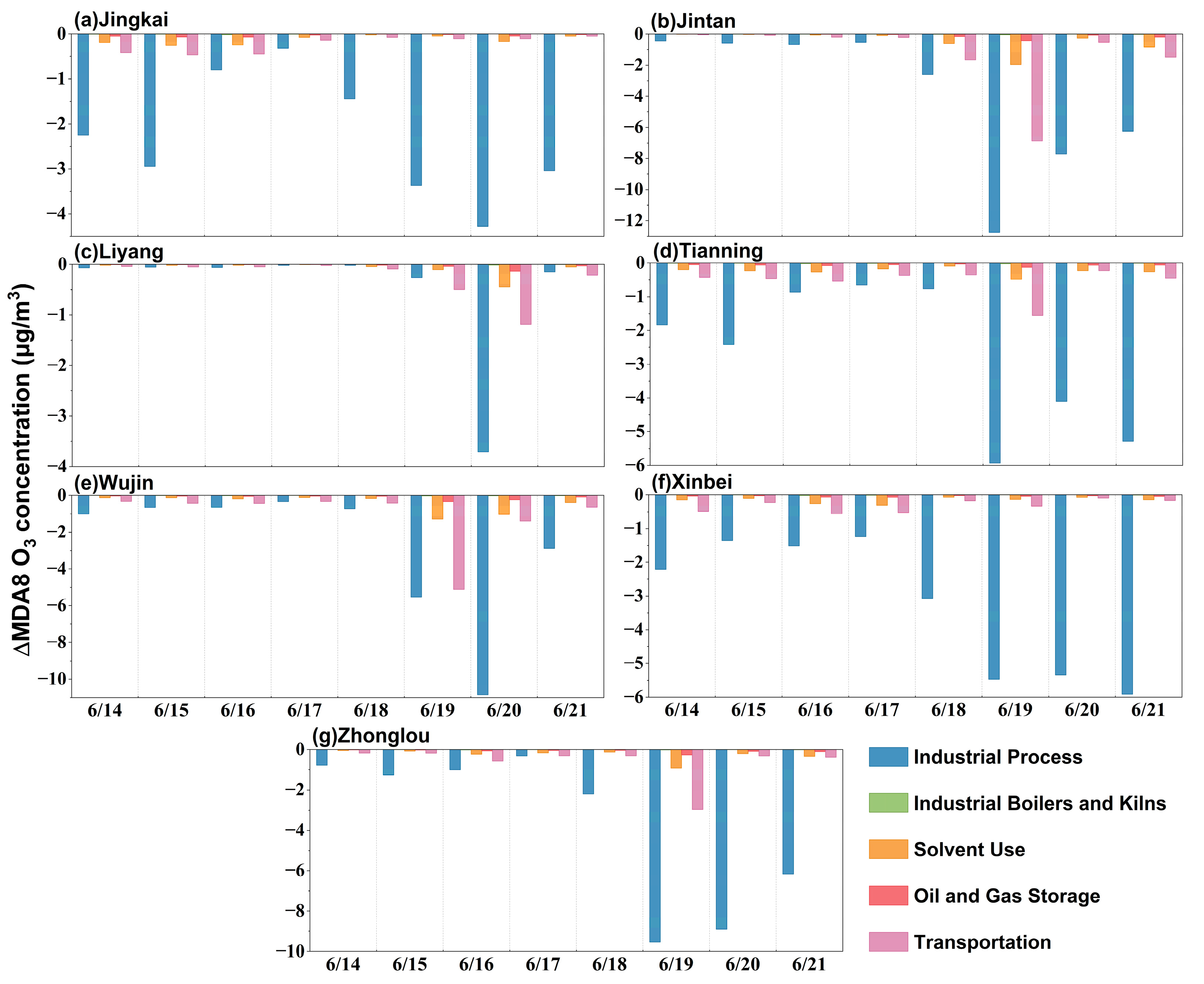
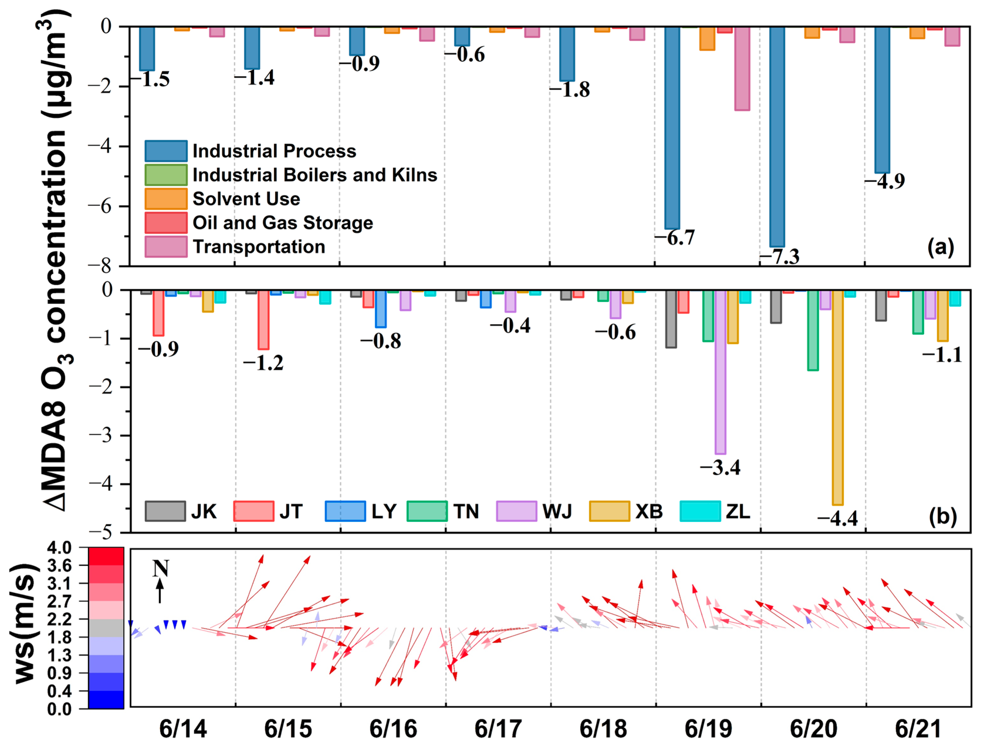
Based on the CMAQ-ISAM results of sectoral contribution, the transportation and industrial processes emerged as the primary contributors to O3 formation, and their average contributions were comparable. A second set of mitigation strategies considers a 40% emission reduction ratio applied to VOC emissions from each source sector across Changzhou. As can be seen in Figure 8a and Figure A10, VOC reductions in industrial processing led to the most substantial ozone decrease (3.2 µg·m−3 on average) during the pollution period, which was consistent with the ISAM results. During the last three days of the pollution period, controlling 40% of VOC emissions from industrial processing resulted in an ozone reduction of over 4.5 µg·m−3. Transportation appeared to be second most effective in reducing ozone concentrations. The averaged MDA8 ozone concentration decreased by 0.7 µg·m−3 if VOC emissions from transportation were reduced by 40%. Reductions in the other sectors resulted in minimal ozone reductions (<0.3 µg·m−3).
In terms of ozone changes at the county level, JT exhibited the most significant ozone reduction following emission control measures (Figure A12). When a 40% reduction in VOC emissions from industrial processes was implemented, the peak decrease in JT’s daily MDA8 O3 concentration reached 12.7 µg·m−3 (3.9 µg·m−3 on average). Furthermore, the average MDA8 ozone concentrations in ZL decreased by 3.7 µg·m−3, particularly during the later stages of the pollution episode, where ozone decreased more noticeably (>6.0 µg·m−3). In contrast, LY experienced the least impact, with a 40% reduction in VOC emissions from various sources resulting in an average MDA8 O3 concentration of no more than 0.5 µg·m−3.

3.2.3. County-Specific Emission Reduction

As demonstrated by the CMAQ-ISAM results in Section 3.1, the O3 contributions from different counties exhibited substantial variations. These discrepancies can be attributed to the differing abundance of emissions sources within each county and the geographical positioning of each county. For instance, during the selected pollution period, particular counties (e.g., TN, ZL, XB) were significantly influenced by emissions from surrounding counties, while other counties (e.g., WJ, JK) were important contributing counties (Figure 5a). Thus, the third set of mitigation strategies focused on evaluating the effectiveness of emission reduction initiatives applied to specific counties within Changzhou. To do so, we implemented a 40% reduction in AVOC emissions for each county at a time and subsequently analyzed the corresponding changes in ozone concentrations for each case. By conducting county-specific emission reduction simulations, we provided a detailed assessment of how targeted emission reductions in specific counties can influence regional ozone levels. This approach allowed for a thorough understanding of the spatial dynamics of ozone pollution and highlights the importance of considering both local and upwind county emissions in developing effective mitigation strategies.
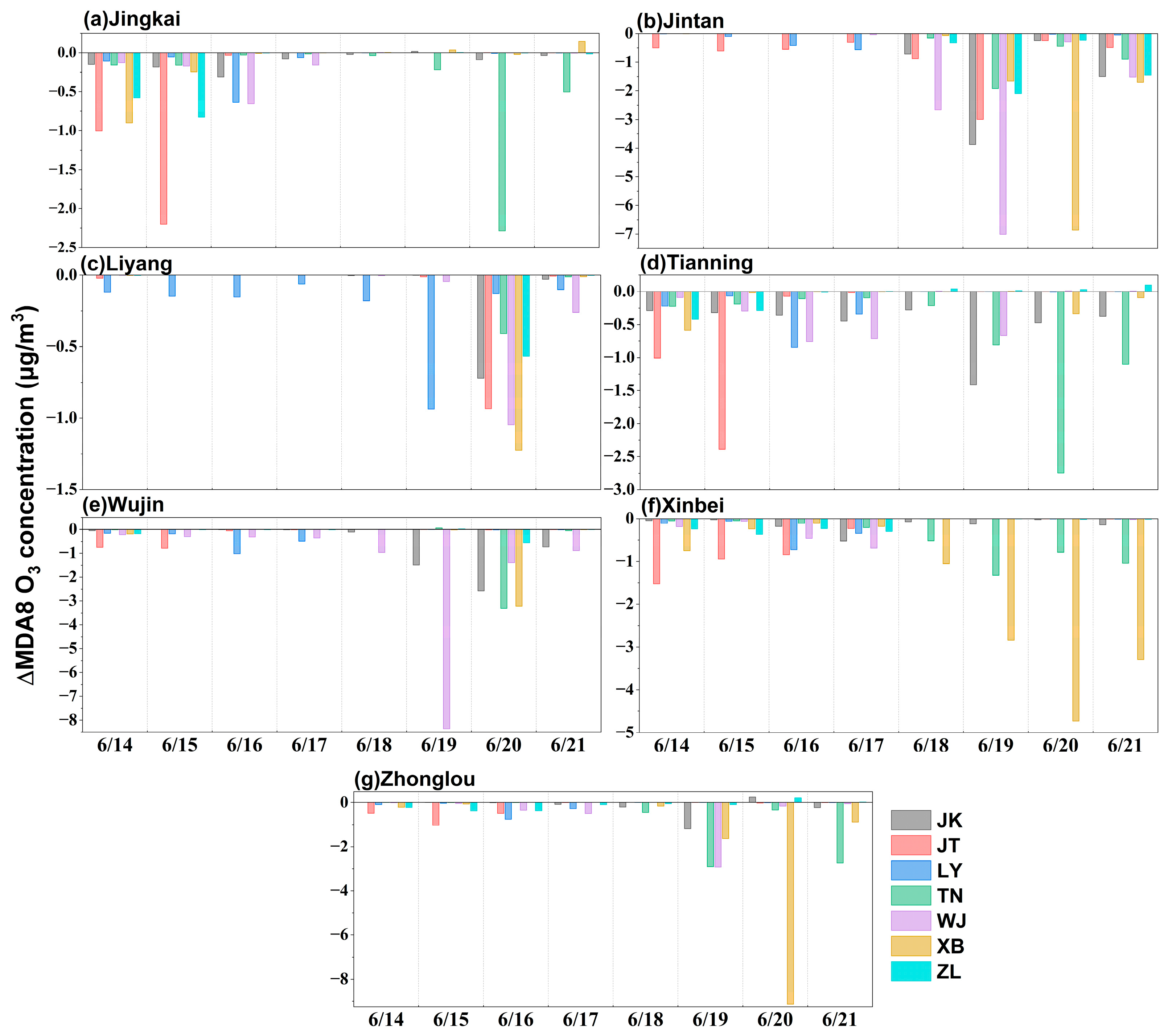
Figure 8b shows the changes in MDA8 O3 concentrations resulting from AVOC reductions across different counties. On average, a 40% AVOC reduction in XB led to the most significant decrease in MDA8 O3 concentration (0.9 µg·m−3) during the pollution episode, whereas the same reduction applied to LY and ZL yielded the least effective outcome (both were 0.2 µg·m−3). However, when evaluating daily effectiveness, no single county consistently emerged as the most effective in terms of control measures. For instance, on June 14th and 15th, AVOC reductions in JT were observed to be the most effective compared to other counties. In the following several days, reductions in WJ led to the largest ozone decrease. During the last two days of the pollution episode, reductions in XB led to the most substantial decrease in ozone concentration. The changing importance of counties to be controlled was primarily associated with the changing wind directions, as controlling emissions within the upwind counties was more effective than controlling the downwind counties. Due to the high emissions in XB, reducing XB emissions yielded the most substantial ozone reduction at regional level (Figure A11), with ozone decreases as much as 4.4 µg·m−3.
In terms of ozone changes at the county level, there was not always a direct correlation between the counties implementing emission reduction measures and those that experienced the resultant effects (as shown by Figure A13). For example, a 40% reduction in VOC emissions in JK resulted in minimal changes to local ozone levels, while the daily MDA8 O3 concentration in JT decreased by 3.9 µg·m−3. Additionally, on 20 June, VOC reduction in ZL led to a rebound in local ozone level. In contrast, LY showed a more pronounced response to local emission reduction strategies, especially during the period from 14 to 19 June. During the last two days of the pollution episode, mitigation strategies in other counties significantly contributed to lowering ozone concentration in LY.

4. Limitations

Several limitations and uncertainties are inherent in the application of this modeling framework, which warrant brief discussion. Firstly, biases present in the WRF-simulated meteorological variables could result in either the underestimation or overestimation of the simulated ozone concentrations. The selection of physical processes and their corresponding parameterization schemes is crucial for the accuracy of meteorological field simulations [49,50]. Among these, the parameterization of the planetary boundary layer (PBL) plays a particularly important role in influencing the simulation results [51,52,53]. Chen et al. [52] employed four different PBL schemes to investigate the seasonal and diurnal variations in typical meteorological variables for the YRD region. Their findings indicated that the MYNN and MYJ schemes performed better in simulating meteorological parameters compared to the YSU and ACM2 schemes. In terms of O3 simulation, Shi et al. [53] found that the YSU scheme was most suitable for the YRD region.
Secondly, uncertainties associated with the emission inventory would also affect model performance. In this study, the MEIC anthropogenic emission inventory was used for the D01 and D02 simulation domains. According to estimates by Zheng et al. [36], pollutants primarily emitted from large sources (e.g., SO2) exhibit relatively low uncertainty (about ±16%). Those associate with more dispersed sources, such as black carbon (BC) and organic carbon (OC), show much higher uncertainty, ranging from −40% to 90%. For the YRD region, the estimated uncertainties in anthropogenic emissions of NOx and VOCs are ±27.7% and ±133.4%, respectively [54]. These uncertainties in anthropogenic emission inventories can directly influence the simulation of pollutant concentrations. Huang et al. [55] suggested that AVOC emissions contributed most to the uncertainty regarding predicted O3 concentrations in coastal regions.
Thirdly, the spin-up period used in most studies is less than or equal to 10 days [55], whereas Hogrefe et al. [56] concluded that a spin-up period of 10 days or one week is insufficient to reduce the influence of initial conditions to below 1%. Our simulation started on 27 May, with a spin-up period of 5 days. To minimize the impact of initial conditions, future simulations should consider extending the spin-up period to 15–20 days.

5. Conclusions

This study provides a methodological, modeling-based framework for developing effective urban ozone pollution control strategies. Using the city of Changzhou as a case study, we demonstrate significant variations in ozone response to different mitigation strategies, highlighting the need for tailored, multi-faceted approaches that consider both sectoral and geographical factors. For sector-specific control strategy, reducing emissions from the industrial process sector yields the most substantial impact, achieving a maximum reduction of 4.2% in MDA8 O3 concentration. For county-specific control strategy, emission reduction in XB and WJ lead to more significant decreases in ozone levels. Further simulations show that in WJ, reducing mobile emissions is more effective than reductions in other sectors, while in XB, the most significant ozone reduction comes from decreasing industrial emissions (Figure A16). However, meteorological conditions cause substantial daily fluctuations in MDA8 ozone reductions. Therefore, emission control strategies should be closely aligned with prevailing wind directions. Future research endeavors should delve deeper into ozone prevention and control strategies by integrating the emission reduction potential of different industries.
Furthermore, the ozone source apportionment analysis shows that the contribution of regional transport is equally important as that of local sources. This finding suggests that local emission reductions alone are insufficient for achieving significant air quality improvements. For instance, a 60% reduction in AVOC emissions within the city of Changzhou (referred to as Case6) resulted in an average ozone decrease of 6.5 µg·m−3 (maximum daily reduction of 15.7 µg·m−3) during the pollution episode. In contrast, a similar 60% reduction in AVOC emissions for the YRD region leads to a markedly greater reduction of 49.0 µg·m−3 (maximum daily reduction of 102.5 µg·m−3). Therefore, while it is imperative to actively promote the reduction in local pollutants, there is also a pressing need to strengthen regional cooperation and implement coordinated emission reductions at the regional level.
While the present work quantifies the ozone response to different mitigation strategies, it does not yet translate these concentration changes into public health benefits or account for the socio-economic feasibility. Extending the framework to include health-impact assessment (e.g., changes in premature mortality) would allow policymakers to weigh air-quality gains against implementation costs. Additionally, coupling the model to cost-effectiveness or cost–benefit modules, for example, considering sector-specific abatement costs, technological readiness, and regulatory enforceability, would highlight which strategies deliver the greatest health benefit per unit investment.

Author Contributions

L.H. and M.N. designed the research. Z.K., C.C. and J.F. collected data. Z.K. performed the CMAQ model computations. L.H., J.T., H.C., L.L. and Y.W. helped with the methods. Z.K. and L.H. wrote the paper with contributions from all co-authors. All authors have read and agreed to the published version of the manuscript.

Funding

This study was supported by the National Key R&D Program of China (No. 2023YFC3708505) and the Changzhou Science and Technology Support Plan (Grant No. CE20235030).

Institutional Review Board Statement

Not applicable.

Informed Consent Statement

Not applicable.

Data Availability Statement

The original contributions presented in the study are included in the article; further inquiries can be directed to the corresponding author.

Acknowledgments

This work is supported by the Shanghai Technical Service Center of Science and Engineering Computing, Shanghai University.

Conflicts of Interest

The authors declare no conflicts of interest.

Abbreviations

The following abbreviations are used in this manuscript:
O3Ozone
PM2.5Fine particulate matter
MDA8 O3Maximum daily 8 h average ozone
YRDYangtze River Delta
CMAQCommunity Multiscale Air Quality Modeling System
ISAMIntegrated source apportionment method
WRFWeather Research and Forecasting
AVOCAnthropogenic VOC
ANOxAnthropogenic NOx
JTJintan
XBXinbei
TNTianning
WJWujin
JKJingkai
LYLiyang
ZLZhonglou
MBMean bias
NMBNormalized mean bias
RCorrelation coefficient
IOAIndex of agreement
TTemperature
RHRelative humidity
WSWind speed

Appendix A

Table A1. Information of national and provincial monitoring stations in Changzhou.
County NameStation NameLongitude/(°)Latitude/(°)
LYYSZZ119.47831.402
DMZZ119.48931.443
WJWJJC119.94631.706
WJJF119.87131.711
JTJTCQ119.59431.728
JTJZJG119.59331.739
JTJC119.60231.758
TNSJC119.96331.762
JKJKQ120.05531.776
ZLZL119.90331.793
XZZX119.98231.817
XBAJ119.92331.908
Table A2. Details of uniform reduction scenarios.
Emission Reduction ScenariosLocal Area of ChangzhouSurrounding Area
Emission Ratio of AVOCsEmission Ratio of NOxEmission Ratio of AVOCsEmission Ratio of NOx
BASE100%100%100%100%
Scen 1100%100%80%80%
Case 1100%80%80%80%
Case 2100%60%80%80%
Case 3100%40%80%80%
Case 480%100%80%80%
Case 560%100%80%80%
Case 640%100%80%80%
Case 780%80%80%80%
Case 860%60%80%80%
Case 940%40%80%80%
Table A3. Details of sector-specific reduction scenarios.
Emission Reduction ScenariosLocal Area of ChangzhouSurrounding Area
Source CategoryEmission Ratio of AVOCEmission Ratio of ANOxEmission Ratio of AVOCEmission Ratio of ANOx
Case 10Industrial Process60%100%80%80%
Case 11Industrial Boilers and Kilns60%100%80%80%
Case 12Solvent Use60%100%80%80%
Case 13Oil and Gas Storage60%100%80%80%
Case 14Transportation60%100%80%80%
Table A4. Details of county-specific reduction scenarios.
Emission Reduction ScenariosLocal Area of ChangzhouSurrounding Area
County NameEmission Ratio of AVOCEmission Ratio of ANOxEmission Ratio of AVOCEmission Ratio of ANOx
Case 15JK60%100%80%80%
Case 16JT60%100%80%80%
Case 17LY60%100%80%80%
Case 18TN60%100%80%80%
Case 19WJ60%100%80%80%
Case 20XB60%100%80%80%
Case 21ZL60%100%80%80%
Table A5. Definition of model performance evaluation metrics used in this study.
No.Statistics IndexDefinition
1Mean bias (MB) M B = 1 N M i O i
2Normalized mean bias (NMB) N M B = 100 % × M i O i O i
3Correlation coefficient (R) R = 1 N M i M ¯ × O i O ¯ 1 N M i M ¯ 2 1 N O i O ¯ 2
4Index of agreement (IOA) I O A = 1 1 N M i O i 2 1 N M i O ¯ + O i O ¯ 2
In the formula, N represents the number of matches between the simulated values of meteorological factors or pollutants involved in the evaluation and the observed values. M i and O i denote the simulated values and corresponding observed values at time i , respectively. M ¯ and O ¯ are the average values of the simulated values and observed values of N meteorological factors or pollutants, respectively.
Table A6. Model performance evaluation of WRF-simulated 2 m temperature (T2), 10 m wind speed (WS10), and relative humidity (RH).
CityMeteorological ParametersObservationSimulationMBNMBRIOA
ChangzhouT2 (°C)28.027.8−0.1−0.4%0.80.9
WS10 (m/s)3.43.70.410.7%0.40.6
RH (%)66.364.0−2.4−3.6%0.80.9
HangzhouT2 (°C)26.927.70.83.0%0.80.9
WS10 (m/s)2.83.10.312.0%0.40.6
RH (%)77.966.7−11.1−14.0%0.80.8
ShanghaiT2 (°C)26.626.1−0.5-2.0%0.90.9
WS10 (m/s)3.73.80.12.0%0.40.7
RH (%)78.672.3−6.2−8.0%0.80.9
NanjingT2 (°C)27.728.71.04.0%0.80.9
WS10 (m/s)3.83.90.12.0%0.50.7
RH (%)66.459.6−6.8−10.0%0.80.8
HefeiT2 (°C)28.028.40.41.0%0.80.9
WS10 (m/s)3.64.00.411.0%0.40.6
RH (%)70.564.7−5.8−8%0.80.8
Table A7. Model performance evaluation for simulated MDA8 O3 in 41 cities in the YRD region during June 2022.
City NameObservation (µg·m−3)Simulation (µg·m−3)MB (µg·m−3)NMB (%)RMSERIOA
Hangzhou129.5117.2−12.3−9.539.00.70.8
Huzhou139.6129.3−10.3−7.439.50.60.7
Jiaxing137.7136.9−0.8−0.639.40.50.7
Jinhua108.9101.3−7.6−734.10.80.8
Lishui101.671.0−30.6−30.138.40.70.7
Ningbo102.499.3−3.1−338.70.50.7
Quzhou100.089.4−10.6−10.627.30.80.8
Shaoxing123.0111.3−1.7−9.535.10.70.8
Taizhou (Zhejiang)96.291.2−5.0−5.230.10.70.8
Wenzhou99.289.6−9.6−9.333.20.70.8
Zhoushan73.480.37.09.528.00.50.7
Shanghai121.5121.80.30.337.50.60.7
Changzhou134.8148.313.610.146.50.50.6
Huai’an128.2150.322.117.347.80.40.6
Lianyungang122.4144.722.318.238.90.70.8
Nanjing143.2141.2−2.0−1.443.00.50.7
Nantong117.9141.824.020.347.80.60.8
Suqian142.0159.917.912.641.70.50.7
Suzhou (Jiangsu)137.7136.6−1.1−0.838.90.60.8
Taizhou (Jiangsu)131.5135.74.23.246.60.40.6
Wuxi134.8145.710.98.140.60.60.8
Xuzhou147.4168.421.014.2500.30.5
Yancheng121.1148.127.022.349.60.60.7
Yangzhou140.9151.510.57.552.70.40.6
Zhenjiang138.5151.913.49.749.40.50.7
Anqing115.0105.2−9.8−8.537.50.60.7
Bozhou145.4164.118.712.850.10.10.4
Chizhou118.5104.0−13.5−11.435.40.70.8
Chuzhou145.9148.72.81.940.90.60.7
Fuyang142.8146.13.32.347.00.20.5
Hefei132.5127.0−5.5−4.137.00.30.6
Huaibei147.0157.110.16.945.00.20.5
Huangshan102.582.8−19.7−19.229.20.80.7
Lu’an128.6122.7−5.8−4.541.20.30.6
Ma’anshan140.1139.1−1.0−0.737.60.50.7
Suzhou (Anhui)141.2152.611.48.142.90.30.6
Tongling109.0105.3−3.7−3.434.40.60.8
Wuhu124.6121.1−3.5−2.832.90.60.8
Xuancheng118.692.9−25.6−21.636.70.70.7
Bengbu146.9154.07.24.942.10.30.6
Huainan140.6139.7−1.0−0.740.50.20.6
Table A8. Parameter settings for the WRF and CMAQ models.
Simulation Region
Horizontal resolution36 km, 12 km, and 4 km
Center longitude and latitude34° N, 110° E
Projection methodLambert conformal conic
WRF
Microphysical processPurdue–Lin
Land surface processNoah land surface model
Planetary boundary layer schemeYonsei University
Long-wave radiationRRTM
Short-wave radiationGoddard
Cumulus convection schemeKain–Fritsch
CMAQ
Gas-phase chemical mechanismCB6
Aerosol moduleAERO7
Initial/boundary conditionsCMAQ default profile
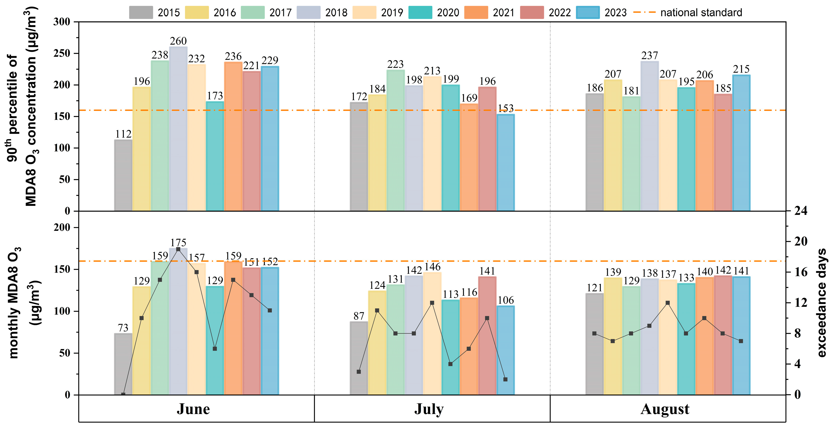
Figure A1. Monthly average of maximum eight-hour ozone (MDA8) concentrations and exceedance days of MDA8 in Changzhou from June to August, 2015 to 2023. The orange dashed lines represents the O3 limits for light and moderate pollution levels, respectively, according to the Ambient Air Quality Standards.
Sustainability 17 07202 g0a1
Figure A2. (a) Regional and (b) sectoral contributions of MDA8 O3 in June 2022.
Sustainability 17 07202 g0a2
Figure A3. Spatial distribution of relative MDA8 ozone contributions between counties when one region was an ozone receptor in June 2022.
Sustainability 17 07202 g0a3
Figure A4. Spatial distribution of relative MDA8 ozone contributions between counties when one region was an ozone source in June 2022.
Sustainability 17 07202 g0a4
Figure A5. Spatial distribution of local ozone sensitivity coefficient to NOx based on CMAQ-DDM simulation. (The highlighted red area represents Changzhou).
Sustainability 17 07202 g0a5
Figure A6. Spatial distribution of local ozone sensitivity coefficient to VOC based on CMAQ-DDM simulation. (The area outlined in blue represents Changzhou).
Sustainability 17 07202 g0a6
Figure A7. Spatial variation in daily MDA8 O3 concentrations under the solo reduction of 20%, 40%, and 60% ANOx emissions in Changzhou from 14 to 21 June 2022. (The area outlined represents Changzhou).
Sustainability 17 07202 g0a7
Figure A8. Spatial variation in daily MDA8 O3 concentrations under the solo reduction of 20%, 40%, and 60% AVOC emissions in Changzhou from 14 to 21 June 2022. (The area outlined represents Changzhou).
Sustainability 17 07202 g0a8
Figure A9. Spatial variation in daily MDA8 O3 concentrations under the reduction of 20%, 40%, and 60% ANOx and AVOC emissions in Changzhou from 14 to 21 June 2022. (The area outlined represents Changzhou).
Sustainability 17 07202 g0a9
Figure A10. Spatial variation in daily MDA8 O3 concentrations under the sector-specific emission reduction in Changzhou from 14 to 21 June 2022. (The area outlined represents Changzhou).
Sustainability 17 07202 g0a10
Figure A11. Spatial variation in daily MDA8 O3 concentrations under the county-specific emission reduction in Changzhou from 14 to 21 June 2022. (The area outlined represents Changzhou. The area outlined in red represents the county that implemented emission reduction).
Sustainability 17 07202 g0a11
Figure A12. MDA8 O3 concentrations changes in seven counties under sector-specific emission reduction scenarios from 14 to 21 June 2022.
Sustainability 17 07202 g0a12
Figure A13. MDA8 O3 concentrations changes in seven counties under county-specific emission reduction scenarios from 14 to 21 June 2022.
Sustainability 17 07202 g0a13
Figure A14. Changes in averaged MDA8 ozone concentrations in Changzhou from 14 to 21 June 2022 under uniform emission reduction scenarios. (The AVOC and NOx emissions in the surrounding area are 100%).
Sustainability 17 07202 g0a14
Figure A15. Changes in MDA8 O3 concentrations with (a) ANOx reduction only, (b) AVOC reduction only, and (c) both reductions in Changzhou from 14 to 21 June 2022. (The AVOC and NOx emissions in the surrounding area are 100%).
Sustainability 17 07202 g0a15
Figure A16. Changes in MDA8 O3 concentrations with a 40% AVOC emissions reduction across different sectors within (a) WJ and (b) XB during 14 to 21 June 2022.
Sustainability 17 07202 g0a16
Figure A17. Daily average MDA8 O3 concentrations and 14:00 Beijing time wind direction in the YRD region from 14 to 21 June 2022. (The blue box lines represent the Changzhou region).
Sustainability 17 07202 g0a17

References

  1. Liang, S.; Chen, Y.; Sun, X.; Dong, X.; He, G.; Pu, Y.; Fan, J.; Zhong, X.; Chen, Z.; Lin, Z. Long-term exposure to ambient ozone and cardiovascular diseases: Evidence from two national cohort studies in China. J. Adv. Res. 2024, 62, 165–173. [Google Scholar] [CrossRef]
  2. Nuvolone, D.; Petri, D.; Voller, F. The effects of ozone on human health. Environ. Sci. Pollut. Res. 2018, 25, 8074–8088. [Google Scholar] [CrossRef] [PubMed]
  3. Wang, B.; Sun, M.; Si, L.; Niu, Z. Spatio-temporal variation of O3 concentration and exposure risk assessment in key regions of China, 2015–2021. Atmos. Pollut. Res. 2024, 15, 101941. [Google Scholar] [CrossRef]
  4. Yan, J.; Wang, X.; Zhang, J.; Qin, Z.; Wang, T.; Tian, Q.; Zhong, S. Research on the spatial and temporal patterns of ozone concentration and population health effects in the Central Plains Urban Agglomeration from 2017 to 2020. PLoS ONE 2024, 19, e0303274. [Google Scholar] [CrossRef]
  5. Bell, M.L.; Zanobetti, A.; Dominici, F. Who is more affected by ozone pollution? A systematic review and meta-analysis. Am. J. Epidemiol. 2014, 180, 15–28. [Google Scholar] [CrossRef]
  6. Jia, H.; Guo, Y.; Luo, H.; Meng, X.; Zhang, L.; Yu, K.; Zheng, X.; Sun, Y.; Hu, W.; Wu, Z. Association of long-term ozone air pollution and age-related macular degeneration in older Chinese population. Sci. Total Environ. 2024, 912, 169145. [Google Scholar] [CrossRef]
  7. Doherty, R.; Wild, O.; Shindell, D.; Zeng, G.; MacKenzie, I.; Collins, W.; Fiore, A.; Stevenson, D.; Dentener, F.; Schultz, M. Impacts of climate change on surface ozone and intercontinental ozone pollution: A multi-model study. J. Geophys. Res. Atmos. 2013, 118, 3744–3763. [Google Scholar] [CrossRef]
  8. Pfister, G.; Walters, S.; Lamarque, J.F.; Fast, J.; Barth, M.; Wong, J.; Done, J.; Holland, G.; Bruyère, C. Projections of future summertime ozone over the US. J. Geophys. Res. Atmos. 2014, 119, 5559–5582. [Google Scholar] [CrossRef]
  9. Shenglan, Z.; Haoyuan, S.; Xingtao, S.; Langchang, J. Impact of urban heat island effect on ozone pollution in different Chinese regions. Urban Clim. 2024, 56, 102037. [Google Scholar] [CrossRef]
  10. Shi, H.; Song, X.; Zeng, S. Impact of the urban heat island effect on ozone pollution in chengdu city, China. Chin. Geogr. Sci. 2023, 33, 1017–1032. [Google Scholar] [CrossRef]
  11. Wang, Y.; Guo, Z.; Han, J. The relationship between urban heat island and air pollutants and them with influencing factors in the Yangtze River Delta, China. Ecol. Indic. 2021, 129, 107976. [Google Scholar] [CrossRef]
  12. Du, S.; He, C.; Zhang, L.; Zhao, Y.; Chu, L.; Ni, J. Policy implications for synergistic management of PM2.5 and O3 pollution from a pattern-process-sustainability perspective in China. Sci. Total Environ. 2024, 916, 170210. [Google Scholar] [CrossRef]
  13. Liu, Y.; Geng, G.; Cheng, J.; Liu, Y.; Xiao, Q.; Liu, L.; Shi, Q.; Tong, D.; He, K.; Zhang, Q. Drivers of increasing ozone during the two phases of clean air actions in China 2013–2020. Environ. Sci. Technol. 2023, 57, 8954–8964. [Google Scholar] [CrossRef] [PubMed]
  14. Liu, Y.; Wang, T. Worsening urban ozone pollution in China from 2013 to 2017–Part 1: The complex and varying roles of meteorology. Atmos. Chem. Phys. 2020, 20, 6305–6321. [Google Scholar] [CrossRef]
  15. Shao, T.; Wang, P.; Yu, W.; Gao, Y.; Zhu, S.; Zhang, Y.; Hu, D.; Zhang, B.; Zhang, H. Drivers of alleviated PM2.5 and O3 concentrations in China from 2013 to 2020. Resour. Conserv. Recycl. 2023, 197, 107110. [Google Scholar] [CrossRef]
  16. Professional Committee on Ozone Pollution Control, Chinese Society for Environmental Sciences. China Blue Book of Atmospheric Ozone Pollution Prevention and Control; Chinese Environmental Science Press: Beijing, China, 2023. [Google Scholar]
  17. Cheng, J.; Tong, D.; Liu, Y.; Geng, G.; Davis, S.J.; He, K.; Zhang, Q. A synergistic approach to air pollution control and carbon neutrality in China can avoid millions of premature deaths annually by 2060. One Earth 2023, 6, 978–989. [Google Scholar] [CrossRef]
  18. Shon, Z.-H.; Kim, K.-H. Impact of emission control strategy on NO2 in urban areas of Korea. Atmos. Environ. 2011, 45, 808–812. [Google Scholar] [CrossRef]
  19. Yang, W.; Chen, H.; Wang, W.; Wu, J.; Li, J.; Wang, Z.; Zheng, J.; Chen, D. Modeling study of ozone source apportionment over the Pearl River Delta in 2015. Environ. Pollut. 2019, 253, 393–402. [Google Scholar] [CrossRef]
  20. Chatani, S.; Morikawa, T.; Nakatsuka, S.; Matsunaga, S.; Minoura, H. Development of a framework for a high-resolution, three-dimensional regional air quality simulation and its application to predicting future air quality over Japan. Atmos. Environ. 2011, 45, 1383–1393. [Google Scholar] [CrossRef]
  21. California Air Resources Board. 2022 State Strategy for the State Implementation Plan. 2022. Available online: https://ww2.arb.ca.gov/resources/documents/2022-state-strategy-state-implementation-plan-2022-state-sip-strategy (accessed on 8 November 2024).
  22. Utah Department of Environmental Quality. UTAH State Implementation Plan. 2019. Available online: https://lf-public.deq.utah.gov/WebLink/DocView.aspx?id=385732&eqdocs=DAQ-2019-005386&cr=1 (accessed on 8 November 2024).
  23. Wang, Y.; Ning, M.; Su, Q.; Wang, L.; Jiang, S.; Feng, Y.; Wu, W.; Tang, Q.; Hou, S.; Bian, J. Designing regional joint prevention and control schemes of PM2.5 based on source apportionment of chemical transport model: A case study of a heavy pollution episode. J. Clean. Prod. 2024, 455, 142313. [Google Scholar] [CrossRef]
  24. Zhao, K.; Wu, Y.; Huang, J.; Gronoff, G.; Berkoff, T.A.; Arend, M.; Moshary, F. Identification of the roles of urban plume and local chemical production in ozone episodes observed in Long Island Sound during LISTOS 2018: Implications for ozone control strategies. Environ. Int. 2023, 174, 107887. [Google Scholar] [CrossRef]
  25. Zhang, Y.; Gao, J.; Zhu, Y.; Liu, Y.; Li, H.; Yang, X.; Zhong, X.; Zhao, M.; Wang, W.; Che, F. Evolution of ozone formation sensitivity during a persistent regional ozone episode in Northeastern China and its implication for a control strategy. Environ. Sci. Technol. 2023, 58, 617–627. [Google Scholar] [CrossRef] [PubMed]
  26. Wang, R.; Wang, L.; Sun, J.; Zhang, L.; Li, Y.; Li, K.; Liu, B.; Zhang, J.; Wang, Y. Maximizing ozone control by spatial sensitivity-oriented mitigation strategy in the Pearl River Delta Region, China. Sci. Total Environ. 2023, 905, 166987. [Google Scholar] [CrossRef] [PubMed]
  27. Tian, J.; Wang, J.; Wang, D.; Fang, C.; Huang, J. Research on ozone pollution control strategies for urban agglomerations based on ozone formation sensitivity and emission source contributions. Environ. Pollut. 2024, 363, 125182. [Google Scholar] [CrossRef]
  28. Li, J.; Wang, Z.; Chen, L.; Lian, L.; Li, Y.; Zhao, L.; Zhou, S.; Mao, X.; Huang, T.; Gao, H. WRF-Chem simulations of ozone pollution and control strategy in petrochemical industrialized and heavily polluted Lanzhou City, Northwestern China. Sci. Total Environ. 2020, 737, 139835. [Google Scholar] [CrossRef]
  29. Changzhou Municipal Bureau of Statistics. Changzhou Statistical Yearbook 2023. 2023. Available online: https://tjj.changzhou.gov.cn/html/tjj/2023/OEJCMFCP_1110/27748.html (accessed on 1 November 2024).
  30. Jensen, A.; Liu, Z.; Tan, W.; Dix, B.; Chen, T.; Koss, A.; Zhu, L.; Li, L.; de Gouw, J. Measurements of volatile organic compounds during the COVID-19 lockdown in Changzhou, China. Geophys. Res. Lett. 2021, 48, e2021GL095560. [Google Scholar] [CrossRef]
  31. Liu, Z.; Xiang, Y.; Pan, Y.; Zhang, T.; Xu, W.; Li, L. Unveiling 3-D evolution and mechanisms of ozone pollution in Changzhou, China: Insights from lidar observations and modelling. Environ. Pollut. 2024, 359, 124556. [Google Scholar] [CrossRef]
  32. Zhang, K.; Liu, Z.; Zhang, X.; Li, Q.; Jensen, A.; Tan, W.; Huang, L.; Wang, Y.; de Gouw, J.; Li, L. Insights into the significant increase in ozone during COVID-19 in a typical urban city of China. Atmos. Chem. Phys. 2022, 22, 4853–4866. [Google Scholar] [CrossRef]
  33. Shu, L.; Xie, M.; Wang, T.; Gao, D.; Chen, P.; Han, Y.; Li, S.; Zhuang, B.; Li, M. Integrated studies of a regional ozone pollution synthetically affected by subtropical high and typhoon system in the Yangtze River Delta region, China. Atmos. Chem. Phys. 2016, 16, 15801–15819. [Google Scholar] [CrossRef]
  34. U.S. EPA. CMAQ, version 5.3.2; United States Environmental Protection Agency: Washington, DC, USA, 2020.
  35. Wang, Y.; Jiang, S.; Huang, L.; Lu, G.; Kasemsan, M.; Yaluk, E.A.; Liu, H.; Liao, J.; Bian, J.; Zhang, K. Differences between VOCs and NOx transport contributions, their impacts on O3, and implications for O3 pollution mitigation based on CMAQ simulation over the Yangtze River Delta, China. Sci. Total Environ. 2023, 872, 162118. [Google Scholar] [CrossRef]
  36. Zheng, B.; Tong, D.; Li, M.; Liu, F.; Hong, C.; Geng, G.; Li, H.; Li, X.; Peng, L.; Qi, J. Trends in China’s anthropogenic emissions since 2010 as the consequence of clean air actions. Atmos. Chem. Phys. 2018, 18, 14095–14111. [Google Scholar] [CrossRef]
  37. Li, L.; Li, Q.; Huang, L.; Wang, Q.; Zhu, A.; Xu, J.; Liu, Z.; Li, H.; Shi, L.; Li, R. Air quality changes during the COVID-19 lockdown over the Yangtze River Delta Region: An insight into the impact of human activity pattern changes on air pollution variation. Sci. Total Environ. 2020, 732, 139282. [Google Scholar] [CrossRef]
  38. Houyoux, M.; Vukovich, J.; Brandmeyer, J.; Seppanen, C.; Holland, A. Sparse Matrix Operator Kernel Emissions Modeling System-SMOKE User Manual; MCNC-North Carolina Supercomputing Center, Environmental Programs, Research Triangle Park: Chapel Hill, NC, USA, 2000. [Google Scholar]
  39. Thunis, P.; Clappier, A.; Tarrasón, L.; Cuvelier, C.; Monteiro, A.; Pisoni, E.; Wesseling, J.; Belis, C.; Pirovano, G.; Janssen, S. Source apportionment to support air quality planning: Strengths and weaknesses of existing approaches. Environ. Int. 2019, 130, 104825. [Google Scholar] [CrossRef] [PubMed]
  40. Tan, Z.; Lu, K.; Jiang, M.; Su, R.; Dong, H.; Zeng, L.; Xie, S.; Tan, Q.; Zhang, Y. Exploring ozone pollution in Chengdu, southwestern China: A case study from radical chemistry to O3-VOC-NOx sensitivity. Sci. Total Environ. 2018, 636, 775–786. [Google Scholar] [CrossRef]
  41. Otero, N.; Sillmann, J.; Mar, K.A.; Rust, H.W.; Solberg, S.; Andersson, C.; Engardt, M.; Bergström, R.; Bessagnet, B.; Colette, A.; et al. A multi-model comparison of meteorological drivers of surface ozone over Europe. Atmos. Chem. Phys. 2018, 18, 12269–12288. [Google Scholar] [CrossRef]
  42. Ye, X.; Wang, X.; Zhang, L. Diagnosing the model bias in simulating daily surface ozone variability using a machine learning method: The effects of dry deposition and cloud optical depth. Environ. Sci. Technol. 2022, 56, 16665–16675. [Google Scholar] [CrossRef] [PubMed]
  43. Kavassalis, S.C.; Murphy, J.G. Understanding ozone-meteorology correlations: A role for dry deposition. Geophys. Res. Lett. 2017, 44, 2922–2931. [Google Scholar] [CrossRef]
  44. Chen, Y.; Wang, M.; Yao, Y.; Zeng, C.; Zhang, W.; Yan, H.; Gao, P.; Fan, L.; Ye, D. Research on the ozone formation sensitivity indicator of four urban agglomerations of China using Ozone Monitoring Instrument (OMI) satellite data and ground-based measurements. Sci. Total Environ. 2023, 869, 161679. [Google Scholar] [CrossRef]
  45. Meng, X.; Jiang, J.; Chen, T.; Zhang, Z.; Lu, B.; Liu, C.; Xue, L.; Chen, J.; Herrmann, H.; Li, X. Chemical drivers of ozone change in extreme temperatures in eastern China. Sci. Total Environ. 2023, 874, 162424. [Google Scholar] [CrossRef]
  46. Mao, Y.-H.; Yu, S.; Shang, Y.; Liao, H.; Li, N. Response of summer ozone to precursor emission controls in the Yangtze River Delta region. Front. Environ. Sci. 2022, 10, 864897. [Google Scholar] [CrossRef]
  47. Liu, Z.; Hu, K.; Zhang, K.; Zhu, S.; Wang, M.; Li, L. VOCs sources and roles in O3 formation in the central Yangtze River Delta region of China. Atmos. Environ. 2023, 302, 119755. [Google Scholar] [CrossRef]
  48. Wang, N.; Lyu, X.; Deng, X.; Huang, X.; Jiang, F.; Ding, A. Aggravating O3 pollution due to NOx emission control in eastern China. Sci. Total Environ. 2019, 677, 732–744. [Google Scholar] [CrossRef]
  49. Xu, L.; Liu, H.; Du, Q.; Xu, X. The assessment of the planetary boundary layer schemes in WRF over the central Tibetan Plateau. Atmos. Res. 2019, 230, 104644. [Google Scholar] [CrossRef]
  50. Li, J.; Yu, S.; Chen, X.; Zhang, Y.; Li, M.; Li, Z.; Song, Z.; Liu, W.; Li, P.; Xie, M. Evaluation of the WRF-CMAQ model performances on air quality in China with the impacts of the observation nudging on meteorology. Aerosol Air Qual. Res. 2022, 22, 220023. [Google Scholar] [CrossRef]
  51. Ma, Y.-F.; Wang, Y.; Xian, T.; Tian, G.; Lu, C.; Mao, X.; Wang, L.-P. Impact of PBL schemes on multiscale WRF modeling over complex terrain, Part I: Mesoscale simulations. Atmos. Res. 2024, 297, 107117. [Google Scholar] [CrossRef]
  52. Chen, D.; Zhu, A.; Huang, L.; Yaluk, E.; Wang, Y.; Ooi, M.C.G.; Gu, Y.; Chan, A.; Li, L. Sensitivity analysis of planetary boundary layer parameterization on meteorological simulations in the Yangtze river delta region, China. Environ. Sci. Atmos. 2024, 4, 1129–1144. [Google Scholar] [CrossRef]
  53. Shi, L.; Zhu, A.; Huang, L.; Yaluk, E.; Gu, Y.; Wang, Y.; Wang, S.; Chan, A.; Li, L. Impact of the planetary boundary layer on air quality simulations over the Yangtze River Delta region, China. Atmos. Environ. 2021, 263, 118685. [Google Scholar] [CrossRef]
  54. Huang, C.; Chen, C.; Li, L.; Cheng, Z.; Wang, H.; Huang, H.; Streets, D.; Wang, Y.; Zhang, G.; Chen, Y. Emission inventory of anthropogenic air pollutants and VOC species in the Yangtze River Delta region, China. Atmos. Chem. Phys. 2011, 11, 4105–4120. [Google Scholar] [CrossRef]
  55. Huang, L.; Zhang, X.; Emery, C.; Mu, Q.; Yarwood, G.; Zhai, H.; Sun, Z.; Xue, S.; Wang, Y.; Fu, J.S. Recommendations on benchmarks for numerical air quality model applications in China–Part 2: Ozone and uncertainty analysis. Atmos. Chem. Phys. 2025, 25, 4233–4424. [Google Scholar] [CrossRef]
  56. Hogrefe, C.; Roselle, S.J.; Bash, J.O. Persistence of initial conditions in continental scale air quality simulations. Atmos. Environ. 2017, 160, 36–45. [Google Scholar] [CrossRef]
Figure 1. Methodological framework for designing ozone emission reduction strategies.
Sustainability 17 07202 g001
Figure 2. (a) The nested modeling domain, (b) the innermost YRD model domain, (c) and locations of the national and provincial monitoring stations in Changzhou. See Table A1 for the locations of the monitoring stations.
Sustainability 17 07202 g002
Figure 3. Spatial distribution of averaged MDA8 O3 for (a) June 2022 and (b) 14–21 June 2022. Observations are represented by colored circles. (c) Time series of simulated and observed hourly O3 concentration in Changzhou, Shanghai, Hangzhou, Nanjing, and Hefei during June 2022. (The wind fields in the figure represent the 14:00 (daily) Beijing time averages for each time period).
Sustainability 17 07202 g003
Figure 4. (a) Regional and (b) sectoral contributions of MDA8 O3 from 14 to 21 June 2022. (c) Relative contributions from surrounding cities and provinces. (d) Time series of observed hourly O3 concentration, wind speed, and direction during the pollution episode.
Sustainability 17 07202 g004
Figure 5. (a) Relative inter-county ozone contributions from 14 to 21 June 2022 (the sum of each row adds up to 100%). (b) Relative ozone contributions to ozone levels in JK. (c) Relative ozone contributions from emissions within JK to other counties.
Sustainability 17 07202 g005
Figure 6. Changes in averaged MDA8 ozone concentrations in Changzhou from 14 to 21 June 2022 under uniform emission reduction scenarios.
Sustainability 17 07202 g006
Figure 7. Changes in MDA8 O3 concentrations with (a) ANOx reduction only, (b) AVOC reduction only, and (c) both reductions in Changzhou from 14 to 21 June 2022.
Sustainability 17 07202 g007
Figure 8. Changes in MDA8 O3 concentrations under (a) sector-specific and (b) county-specific emission reduction scenarios during 14–21 June 2022.
Sustainability 17 07202 g008
Table 1. Summary of different mitigation scenarios (see Table A2, Table A3 and Table A4 for details).
Mitigation ScenarioNOx/AVOC EmissionsSectorsCountiesSimulations
Uniform emission reductionReduction ratio (20%, 40%, 60%) applied to NOx and/or AVOCAll sectorsAll countiesCase 1–Case 9
Sector-specific reductionOnly reducing AVOC by 40%One sector at a timeAll countiesCase 10–Case 14
County-specific reductionOnly reducing AVOC by 40%All sectorsOne county at a timeCase 15–Case 21
Disclaimer/Publisher’s Note: The statements, opinions and data contained in all publications are solely those of the individual author(s) and contributor(s) and not of MDPI and/or the editor(s). MDPI and/or the editor(s) disclaim responsibility for any injury to people or property resulting from any ideas, methods, instructions or products referred to in the content.