Can Regional Infrastructure Predict Its Economic Resilience? Limited Evidence from Spatial Modelling

Abstract

This study examines whether regional infrastructure can predict economic resilience in European regions, focusing on resistance, recovery, and reorientation during the COVID-19 crisis. While infrastructure is widely recognized as a key factor influencing regional resilience, its explicit role has been underexplored in the European context. Using a comprehensive literature review and spatial econometric models applied to NUTS-2 level data from 2017 to 2024, we investigate the direct and spatial spillover effects of various infrastructure types—transportation, healthcare, tourism, education, and digital access—on regional resilience outcomes. We apply OLS and four spatial models (SEM, SLX, SDEM, SDM) under 29 spatial weighting matrices to account for spatial autocorrelation. Results show that motorway density, early school leaving, and healthcare infrastructure in neighbouring regions significantly affect resistance. For recovery, railway density and GDP per capita emerge as key predictors, with notable spatial spillovers. Reorientation is shaped by population structure, railway density, and tourism infrastructure, with both positive and negative spatial dynamics observed. The findings underscore the importance of infrastructure not only in isolation but also within regional systems, revealing complex interdependencies. We conclude that policymakers must consider spatial externalities and coordinate infrastructure investments to enhance regional economic resilience across interconnected Europe.

1. Introduction

The previous two decades have witnessed crises and instability worldwide, but no one was prepared for the global pandemic at the start of 2020. Since then, although the pandemic has subsided, the world has faced continuous and overlapping crises and shocks [1,2], such as supply chain disruptions, energy shortages, wars, and shifts in global economic policies.

While not all pandemic- or economy-driven crises directly affect infrastructure, one could argue that they significantly increase or decrease regional resilience in the face of any shock. Based on the literature from around the world [3,4,5,6,7], infrastructure can be seen as a moderating factor in regional economic resilience; however, in the case of Europe, the role of infrastructure in regional economic resilience has not been thoroughly explored in recent years despite numerous major events that have directly impacted the continent. As a result, policymakers may risk overlooking or underestimating key drivers of regional economic resilience during periods of economic turbulence.

To examine the role of infrastructure on economic resilience, we conducted a literature review following the methodology outlined by [8], which involved multiple searches through the Scopus and Web of Science databases for empirical articles published between 2019 and 2024. During the selection process, we excluded non-empirical articles, articles not focusing on Europe, and articles that do not describe resilience as a multidimensional phenomenon. Based on this review, we determined major categories of factors (including infrastructure) that influence regional economic resilience.

Regional economic resilience highlights various determinants that shape how regions’ economies resist, recover, and transform in response to shocks [9]. Economic structure [10,11], spatial connectivity [12,13,14], and innovation systems [14,15] influence a region’s adaptive capacity and ability to redirect growth. Human capital [13,16,17], labour dynamics [16,18], and demographic trends [10,19] determine workforce flexibility and long-term renewal. Governance quality [13], access to capital [14,20], and development level [19,21] set the institutional and financial foundations for resilience. Trade openness [22] and output scale [21] affect vulnerability and recovery speed, while entrepreneurship [23] drives renewal through firm dynamism. Though less frequently studied, healthcare and social cohesion [21] can also support societal stability and community-based responses.

Although only a few articles [14,16,24] have directly examined infrastructure as a determinant of regional economic resilience in Europe, it is possible that several indicators categorised under Spatial, Health, or Economic Structure also reflect infrastructure. When these broader measures are considered, infrastructure-related influences become even more pronounced. The literature consistently shows that a well-developed infrastructure base contributes positively to all phases of resilience [3,5,6]: resistance, recovery, and long-term reorientation. This aligns with the view that regional economies function as complex adaptive systems where local interactions, historical trajectories, and path-dependent processes shape uneven development and adaptability [25,26]. Nevertheless, our literature review suggests that the explicit incorporation of infrastructure in empirical research on regional economic resilience remains underutilised.

Taking all of this into account, we identify infrastructure as a significantly under-researched factor in the context of regional economic resilience in Europe in recent years. By applying spatial modelling techniques, we aim to determine which types of infrastructure should be prioritised by policymakers seeking to strengthen regional resilience.

This study investigates the dimensions of regional economic resilience—resistance, recovery, and reorientation—across European NUTS-2 regions, with a particular focus on the role of infrastructure. While the literature acknowledges infrastructure as a component of resilience, this research will be one of the few systematic and empirical examinations of infrastructure within regional economic resilience. Addressing this gap, we analyse the period from 2017 to 2024, with emphasis on the context of the COVID-19 pandemic, which, according to the literature, is still less researched compared to the 2008 Great Recession and can provide new valuable insights [27]. We calculate resilience dimensions using a sensitivity index and introduce an innovative method to measure reorientation based on high-tech employment. This novel approach allows us to compare all resilience dimensions consistently, ensuring comparability across resistance, recovery, and reorientation measures. While previous studies often apply a variety of spatial models or weighting matrices, we take this approach further by systematically combining 29 spatial weighting matrices with four spatial models (SEM, SLX, SDEM, SDM), applying each matrix across all models. Following initial exploration with OLS and Moran’s I, this comprehensive spatial analysis allows us to robustly capture spatial dependencies and examine how infrastructure and other factors influence resilience across diverse spatial contexts.

The rest of the paper is structured as follows: Section 2.1 outlines the use of Ordinary Least Squares (OLS), Moran’s I statistic, and various spatial weighting schemes to assess whether spatial dependencies should be considered in the econometric analysis, and it also introduces the baseline equation used in this study; Section 2.2 describes the spatial econometric models applied in the research, explains their differences, and presents modifications to the initial equation to accommodate each model; Section 2.3 defines the concept of regional economic resilience, detailing its key dimensions and how they are measured; Section 2.4 provides a comprehensive overview of the variables used to explain resilience, including data sources and descriptive statistics; Section 3.1 presents Moran’s I results across all resilience dimensions and spatial weight matrices; Section 3.2, Section 3.3 and Section 3.4 report findings for the resistance, recovery, and reorientation dimensions using all specified models; Section 4.1, Section 4.2 and Section 4.3 discuss policy recommendations for strengthening regional resistance, recovery, and reorientation; Section 4.4 outlines the study’s limitations and proposes directions for future research.

2. Materials and Methods

2.1. OLS Model, Moran’s I, and Spatial Weighting Schemes

Our paper aims to model the link between regional economic resilience and its infrastructure. We begin our methodological framework with a simple OLS specification:

$$r=\mathit{X}\beta +e,$$

(1)

where r is an n × 1 vector of observations of the resilience variable, X is an n × k matrix of resilience factors (including infrastructure), β is a k × 1 vector of regression coefficients, e is a normally distributed, independent, and identically distributed error term, n is the number of NUTS2 regions, and k is the number of regressors.

The assumption of e~N(0, σ²I) is doubtful, and e is probably a subject of spatial autocorrelation given that a region exists not in isolation but in a complex interrelation with other regions. This is true not just in the case of regions within a particular country but also between countries because, in the EU, countries’ economic borders are irrelevant. Thus, we will compute Moran’s I on the residuals e of the OLS estimation of Equation (1) using different types of spatial weight matrices W. This will allow us to identify whether significant spatial autocorrelation remains after estimating OLS regression [28], and which W allows us to identify the most suitable spatial structure for Equation (1), since spatial autocorrelation might be evident with one weighting scheme but not another, influencing the choice of spatial model specification. Moran’s I tests across multiple spatial weight matrices increase robustness, ensuring that spatial dependence is not sensitive to arbitrary choices of spatial structures.

As highlighted in the literature [29,30,31], considerable debate persists regarding the importance or relative insignificance of selecting an appropriate spatial weight matrix. Moreover, the wide variety of available types and configurations further complicates the choice of the most suitable matrix. Therefore, we will examine three commonly used types of spatial weight matrices. The first type is contiguity-based weights [28], identifying regions as neighbours if they share common borders. This is particularly relevant in EU NUTS2 regions, as administrative boundaries are clearly defined. Rook contiguity considers two regions’ neighbours if they share a common edge (border). For example, if two NUTS2 regions share a common administrative boundary (not merely a corner), they are neighbours under the Rook criterion, ignoring corner connections and possibly missing some spatial interactions. Queen contiguity considers two regions as neighbours if they share a common edge or corner (vertex). Thus, accounting for bordering and diagonal (vertex-connected) NUTS2 regions, Queen contiguity becomes more inclusive than Rock, capturing more faint or indirect spatial effects; however, at the same time, it includes potentially weaker connections (only corner-shared), which may not represent genuine spatial spillovers.

The second type is distance-based weights, which define neighbours based on geographic proximity, measured by centroids or actual distances between regions:

$$W_{ij}=\left\{\begin{array}{ll}1,& if d_{ij}\le d^{*}\\ 0,& if d_{ij}>d^{*}\end{array}, \right.$$

(2)

where d_ij is the distance between the centroids of regions i and j, and d^* is a threshold distance. Following recommendations in the literature that suggest spatial spillover effects typically range from 200 to 1000 km and can extend as far as 3000 km [32], our research defines neighbours based on threshold distances of 200, 500, and 1000 km interregional distance.

This framework explicitly captures spatial decay in interactions and is helpful for large or heterogeneous NUTS2 regions. Still, it is sensitive to the threshold distance choice. It does not expressly account for regional boundaries, potentially linking geographically close but practically disconnected regions (i.e., separated by mountains or water bodies).

The third type is k-nearest neighbours (k-nn) weights [33], which define a fixed number (k) of nearest regions as neighbours based on distance ranking:

$$W_{ij}=\left\{\begin{array}{ll}1,& if region j is among the k closest neighbours to region i\\ 0,& otherwise\end{array}. \right.$$

(3)

In this framework, each region, irrespective of its size or location, has the same number of neighbouring regions, ensuring uniformity in connectivity, which is particularly useful when regional densities vary significantly [33]; however, if the regional density is low, it arbitrarily forces distant regions into neighbour relations, and spatial interaction might be underestimated or overestimated depending on the chosen k. To address the latter, we calculate Moran’s I for k ranging from 1 to 24 [34].

Thus, for 29 types of W, we calculate Moran’s I statistics on the obtained OLS residual e from the non-spatial specification Equation (1):

$$I={\displaystyle \frac{n}{S_0}}{\displaystyle \frac{e\prime \mathit{W}e}{e\prime e}},$$

(4)

where I is a global measure of spatial autocorrelation assessing whether similar (or dissimilar) values are clustered in space; $S_0={\sum }_{i=1}^n{\sum }_{j=1}^n{W}_{ij}$ is a sum of all elements in the spatial weight matrix, which acts as a scaling factor to adjust for the total amount of spatial connectivity; W is n × n spatial weight matrix where each element W_ij reflects the spatial relationship between region i and region j; $e\prime \mathit{W}e$ is the spatial cross-product of residuals, which measures the degree to which residuals at region i are systematically related to residuals at region j across space, weighted by W_ij; and $e\prime e$ is the sum of squared residuals, which serves as a normalisation term, ensuring that Moran’s I is appropriately scaled and comparable across different types of resilience.

I > 0 signals positive spatial autocorrelation, i.e., similar values cluster together (i.e., high-high or low-low resilience regions). I < 0 indicates negative spatial autocorrelation, i.e., dissimilar values are neighbouring (i.e., high-low resilience contrasts). If I ≈ 0, no meaningful spatial autocorrelation is present. A significant Moran’s I would suggest using the spatial model.

2.2. Spatial Models

The simplest spatial model is the Spatial Error Model (SEM), which assumes spatial dependence in the error term rather than in the resilience or its factors [35]. Spatial dependence might arise from omitted variables or measurement errors that are spatially correlated. To estimate SEM, we will use a general specification (1). Still, with a composite error term, that is e = λWe + ε, ε~N(0, σ²I), where e is the spatially dependent error term, λ is the spatial autoregressive parameter indicating spatial error dependence, and ε is a normally distributed, independent, and identically distributed error term. Thus, SEM would generally focus in our research on unobserved spatial heterogeneity and omitted variables influencing spatial correlation in errors.

The Spatial Lagged Exogenous Variables Model (SLX) incorporates spatially lagged resilience factors but does not explicitly model spatial dependence in the resilience or the error term [36]. It allows us to measure how neighbouring regions’ resilience factors affect local resilience. Our specification of SLX is as follows:

$$r=\mathit{X}\beta +\mathit{W}\mathit{X}\gamma +\epsilon ,$$

(5)

where WX are the spatially lagged resilience factors, and γ represents the vector of coefficients associated with the spatially lagged resilience factors. Thus, SLX isolates spillover effects from resilience factors, emphasising neighbourhood influences without direct spatial autocorrelation in resilience. It is especially relevant in the context of our research given that infrastructure such as roads, railways, etc., does not stop at a region’s border, and its effect on resilience may strongly depend on what infrastructure is in the surrounding regions since there is no such thing as isolated infrastructure within regional borders that would be useful for the region’s economy.

The Spatial Durbin Error Model (SDEM) combines the SEM and SLX, incorporating spatial dependence in the error term and spatially lagged resilience factors, thus capturing omitted spatially correlated variables and direct neighbourhood effects [29]. Our specification of SDEM is as follows:

$$r=\mathit{X}\beta +\mathit{W}\mathit{X}\gamma +e,$$

(6)

where e, as previously, is the spatially dependent error term that is decomposed as λWe + ε, ε~N(0, σ²I). This way, SDEM captures omitted spatial influences (through errors) and spillover effects from resilience factors.

The Spatial Durbin Model (SDM) explicitly includes spatial dependence in resilience and its factors. This specification distinguishes between direct and indirect (spatial spillover) effects [29]. Our specification of SDM is as follows:

$$r=\rho \mathit{W}r+\mathit{X}\beta +\mathit{W}\mathit{X}\gamma +\epsilon ,$$

(7)

where Wr is the spatially lagged resilience, and ρ represents the spatial autoregressive parameter indicating the strength of dependence in the resilience. This way, SDM allows the estimation of both endogenous spatial spillovers from the resilience and exogenous spatial spillovers from resilience factors.

The model estimations were implemented using custom code written in Python 3.13.2. We used the following libraries: libpysal, spreg, statsmodels, numpy, pandas, and geopandas; we worked in the PyCharm integrated development environment. The shapefiles for the Territorial Units for Statistics (NUTS) were obtained from the Eurostat GISCO database. The configurations used were the NUTS 2016 version, polygon (RG) geometry, 1:20 million scale, and the EPSG:3035 coordinate reference system.

2.3. Measuring Resilience

To measure regional economic resilience r, we will use three perspectives: Resistance (Rsis), Recovery (Rcov), and Reorientation (Rori).

In the context of regional economic resilience, resistance refers to the ability of a region to withstand or absorb shocks or disruptions without experiencing substantial decline or structural change [9]. This involves the regional economic systems’ inherent robustness and ecological resilience [37,38], which provide them with the capacity for shock absorption and the maintenance of stability and durability in the face of adverse conditions. Resistance emphasises the structural strength and stability that allow a region to continue functioning effectively, avoiding significant negative impacts when confronted with economic disturbances.

In the context of regional economic resilience (also known as engineering resilience), recovery describes a region’s capability to quickly return to a pre-existing state or level of economic functioning following a disruption [37,38]. This capability underscores the region’s potential to bounce back, swiftly rebound, and achieve restoration, effectively ensuring a return to equilibrium [39]. Recovery thus highlights the speed and effectiveness with which a region can restore its economy to its original condition following a shock [9], focusing on restoration rather than structural change or adaptation.

In the context of regional economic resilience, reorientation reflects a region’s capacity to recover, adapt, transform, or even improve its economic structures and processes in response to disruptions or evolving conditions [8,40,41,42]. Known variously as adaptive or transformative resilience, this concept captures a region’s capacity for adaptation and renewal. It encompasses the ideas of bounce-forward and bounce-beyond, highlighting the region’s potential for reconfiguration, innovation, and evolutionary change. Reorientation stresses the importance of adaptive change, emphasising the region’s ability to utilise disruptions as opportunities for transformation and improvement, actively shaping a new, frequently enhanced economic path rather than merely restoring previous conditions.

We will employ the sensitivity index (SI) to measure resilience in all three cases [9,38,43]. For resistance and recovery, we will use the total employment rate (TE) and, for reorientation, employment in high-technology sectors (high-technology manufacturing and knowledge-intensive high-technology services) as a percentage of total employment (HTE). Since we are testing our model targeting the COVID-19 crisis, we will consider 2017–2019 as the pre-crisis period, 2020–2021 as the COVID-19 crisis, and 2022–2024 as the post-COVID-19 period. Following recent developments in the literature, we introduce a slight modification to the classical sensitivity index: rather than comparing NUTS-2 regional levels to national averages, we compare regional performance directly against the broader European context [44,45]. We calculate resistance (Rsis) using the sensitivity index as follows:

$${SI}_{Rsis,i}={\displaystyle \frac{\left(E_{i,2020-2021}^{low}-E_{i,2017-2019}^{high}\right)/E_{i,2017-2019}^{high}}{\left(E_{EU,2020-2021}^{low}-E_{EU,2017-2019}^{high}\right)/E_{EU,2017-2019}^{high}}},$$

(8)

where $E_{2020-2021}^{low}$ is the lowest employment rate over the crisis period in region i and EU27, and $E_{2017-2019}^{high}$ is the highest employment rate over the pre-crisis period in region i and EU27.

We calculate recovery (Rcov) using the sensitivity index as follows:

$${SI}_{Rcov,i}={\displaystyle \frac{\left({E_{i,2022-2024}^{high}-E}_{i,2020-2021}^{low}\right)/E_{i,2020-2021}^{low}}{\left({E_{EU,2022-2024}^{high}-E}_{EU,2020-2021}^{low}\right)/E_{EU,2020-2021}^{low}}},$$

(9)

where $E_{i,2022-2024}^{high}$ is the highest employment rate over the post-crisis period in region i and EU27.

We calculate reorientation (Rori) using the sensitivity index as follows:

$${SI}_{Rori,i}={\displaystyle \frac{\frac{\left({{HTE}_{i,2022-2024}^{high}-HTE}_{i,2020-2021}^{low}\right)}{{HTE}_{i,2020-2021}^{low}}}{\frac{\left({{HYE}_{EU,2022-2024}^{high}-HTE}_{EU,2020-2021}^{low}\right)}{{HTE}_{EU,2020-2021}^{low}}}}.$$

(10)

Table 1. Interpretation of sensitivity indices.

SI Value	Resistance (Rsis)	Recovery (Rcov)	Reorientation (Rori)
>1	The region’s employment rate decreased more than in the EU27	The region’s employment rate recovered faster than in the EU27	The region’s employment share in the high-tech sector increased faster than in the EU27
=1	The region’s employment rate trend is the same in the EU27	The region’s employment rate recovery is the same as in the EU27	The region’s employment share in the high-tech sector changed as in the EU27
<1	The region’s employment rate decreased less than in the EU27	The region’s employment rate recovered more slowly than in the EU27	The region’s employment share in the high-tech sector increased less than in the EU27
=0	The region’s employment rate did not change at all	The region’s employment rate did not recover	The region’s employment share in the high-tech sector did not change
<0	The region’s employment rate changed in the opposite direction to that of EU27	The region’s employment rate changed in the opposite direction to that of EU27	The region’s employment share in the high-tech sector changed in the opposite direction to that of EU27

presents the interpretation of all three sensitivity indices. In addition, Figure A1, Figure A2 and Figure A3 in Appendix A.1 illustrate the results for the resistance, recovery, and reorientation sensitivity indices, respectively.

2.4. Infrastructure and Other Resilience Determinants

The matrix of resilience factors X includes a variety of infrastructure variables that represent different types of infrastructure in the NUTS2 regions. We use the average over 2017–2019 for these variables to proxy pre-crisis regional conditions. Exceptions are made for the population age structure, which uses data from 2021, and the government quality index, which relies on data from 2017.

As it is common to represent transportation infrastructure, we use a motorway (MD) and a railway (RD) density measured as kilometres per 1000 sq. kilometres [46]. Here, we assume that higher densities correlate with better accessibility, as more kilometres of infrastructure per given area implies easier and more convenient access to transportation networks. Good accessibility is crucial for economic activities, influencing trade, investment, and regional development [47,48]. Higher-density regions usually have a more comprehensive network coverage, enhancing connectivity. Dense infrastructure networks can reflect effective spatial planning and efficient resource allocation [49].

To represent tourism infrastructure, we use tourism beds (TB) [50], which include beds in hotels, holiday and other short-stay accommodations, camping grounds, recreational vehicle parks, and trailer parks per 100,000 people. Tourism beds indicate a region’s capacity to accommodate tourists [51]—a fundamental aspect of tourism infrastructure. A higher number indicates a stronger potential for handling tourism flows. Regions with more beds per capita typically have better-developed hospitality sectors, translating into enhanced visitor experiences, more extended tourist stays, and potentially higher tourism expenditure. This metric signals the economic maturity and readiness of a region to benefit economically from tourism, including job creation, local business growth, and overall economic activity generated by visitors. Higher tourism bed densities may also indicate regions specialised in tourism, suggesting greater economic dependency on tourism and potential economic vulnerability, which can shape regional economic resilience.

We use available hospital beds (HB) per 100,000 people to represent healthcare infrastructure [5]. The number of hospital beds directly reflects the healthcare system’s capacity to deliver inpatient care [52], handle emergencies, manage chronic and acute conditions, and respond to public health crises. Higher bed availability indicates a region’s greater preparedness and resilience to healthcare demands and emergencies, such as pandemics or natural disasters. Regions with higher hospital bed densities are typically better equipped to provide timely and adequate medical services, improving accessibility to healthcare services. Sufficient hospital bed numbers often correlate with broader healthcare infrastructure quality, including available specialised medical services, equipment, and qualified medical personnel. Bed density can reflect the efficiency and adequacy of health systems, influencing overall population health outcomes and healthcare accessibility. Adequate hospital bed provision contributes positively to public health outcomes, indirectly influencing productivity, quality of life, economic growth, and regional attractiveness for residents and businesses. Particularly significant during public health emergencies (pandemics like COVID-19), hospital bed availability directly impacts a region’s resilience and capacity to handle surges in healthcare demand.

To represent the information and communication infrastructure, we use the percentage of households with access to the internet at home (IE). A higher percentage signals the extent to which a reliable and modern communication infrastructure has been deployed and is accessible across a region. Home internet access is critical for participating in the digital economy, including e-commerce, teleworking, online education, e-government services, and telemedicine. Regions with higher household internet access typically show stronger economic development and innovation capacities [53]. This indicator captures not only the availability but also the social inclusiveness of communication infrastructure, as disparities in access often mirror broader inequalities in income, education, and geographic location [54]. Internet access at home has become a basic necessity, comparable to utilities such as water and electricity, and is crucial for social participation and information access. A high household internet access rate suggests the widespread adoption of modern technologies, supporting broader communication service expansions such as 5G networks, smart grids, and IoT applications. It indicates a region’s readiness to leverage advanced technological applications, facilitating innovation, research, and smart regional development.

We use the percentage of early leavers from education and training (EdL) aged 18–24 to represent the education infrastructure. A lower percentage of early leavers suggests that the education system effectively retains students, provides relevant and accessible education, and supports students in completing their studies. High rates of early leaving often indicate systemic weaknesses in the education infrastructure, such as insufficient support services, inadequate school facilities, or limited access to vocational or alternative education pathways. Early leaving rates reflect how accessible and inclusive the education infrastructure is for different social, economic, and geographic groups. Higher early leaving rates may signal barriers such as poor transportation to schools, lack of affordable post-secondary education options, or inadequate technological infrastructure (e.g., lack of digital learning tools). Education infrastructure plays a critical role in developing human capital [55]. Regions with lower early leaving rates tend to have a better-educated workforce, which supports higher productivity, innovation, and economic growth. Early school leavers face higher risks of unemployment [56], lower income, and social marginalisation, making this indicator highly relevant for evaluating the broader socio-economic effectiveness of education infrastructure. A low early leaving rate often reflects that schools and training institutions offer high-quality, relevant, and engaging educational programs that meet the needs and expectations of young people. It also suggests that the education system is flexible and can provide diverse pathways, including vocational training, apprenticeships, and higher education alternatives. Variations in early leaving rates between regions reveal disparities in the strength and accessibility of education infrastructure.

In X, we also include the European Quality of Government Index (QoG) and population density (POPD) measured as the number of people per sq. kilometre. They are good proxies for the overall quality and quantity of regional infrastructure [57]. High-quality governments are better at planning, prioritising, and implementing infrastructure projects coherently and in a forward-looking manner. Good governance ensures that public investments in infrastructure are made based on needs assessments, cost-benefit analyses, and long-term regional development goals. Quality government institutions build new infrastructure and maintain and upgrade existing assets, ensuring long-term sustainability [58]. Lower levels of corruption result in infrastructure investments being used as intended, avoiding issues such as cost overruns, substandard construction, or misallocation. Regions with high government quality are better positioned to attract private investment in infrastructure through public–private partnerships, reducing fiscal pressure and improving efficiency. Trust in government facilitates citizen support for infrastructure projects and minimises resistance to necessary but disruptive investments (e.g., large transport hubs and energy projects).

In densely populated regions, infrastructure can be built and operated more cost-effectively because fixed costs (e.g., roads, water supply, public transport) are spread over a larger population. High-density areas have concentrated demand, justifying investments in complex and high-capacity infrastructure [59], such as metro systems, high-speed internet, specialised hospitals, and significant education centres. Densely populated regions often require more sophisticated infrastructure systems to efficiently manage congestion, environmental stress, public health, and urban services; however, a very high density can also lead to overburdened systems (i.e., traffic congestion [60], overloaded sewage systems) if infrastructure investment does not keep pace with population growth. Higher density demands better spatial coordination and integration of infrastructure networks (i.e., linking housing with transport and utilities), increasing the complexity of infrastructure planning.

To capture regional heterogeneity in terms of other factors affecting regional economic resilience and to reduce the likelihood of omitted variable bias, X includes GDP at current market prices PPS per inhabitant (Y) to proxy regional development level, population 0–24 years and population 65 years or over to population 25–64 years (PAS) to proxy regions’ population age structure, and population (POP) to proxy the region’s size.

Per capita GDP is a direct proxy of a region’s economic development [44], industrial diversification, labour productivity, and market integration. It also might indirectly capture a range of factors strongly associated with economic resilience, such as investment in human capital (education, training), technological adoption and innovation capacity, entrepreneurial activity and business density, and broader financial, labour, and goods market efficiency. Including GDP per capita, we can control for a composite measure of economic health and complexity that underlies many resilience-related characteristics, thereby reducing the risk that unobserved heterogeneity in development levels biases the estimated effects of infrastructure characteristics.

Young and elderly people, relative to the working-age population (dependency ratio), directly capture the demographic burden on productive segments of society. It directly proxies labour market pressure [44], public service demand (education, healthcare), and future labour force potential. It also might indirectly reflect long-term growth prospects (younger populations imply future labour supply), fiscal sustainability (ageing populations may stress pensions and healthcare systems), innovation potential (younger populations often correlate with higher adaptability and technology adoption), and social cohesion and vulnerability (regions with extreme age structures may be more vulnerable to shocks). By accounting for the age structure, we control for a major source of regional economic heterogeneity that affects resilience [61], particularly in how regions respond to labour market shocks, adapt to demographic changes, and manage social support systems.

The absolute population size proxies the scale of the region, which has direct and indirect implications for economic resilience. It directly proxies the size of the labour market, local consumer market, economies of agglomeration (benefits from the concentration of people and activities) [62], and the capacity to achieve scale economies in public infrastructure and services. It indirectly captures urbanisation level, complexity and diversity of economic activities, the potential for network effects (e.g., innovation clusters, knowledge spillovers), and political bargaining power for national investments. Regions of different sizes inherently differ in their capacity to absorb shocks, diversify economic bases, and maintain essential public services. Controlling for population size thus prevents confounding the analysis of resilience with simple side effects.

All in all, X = {ln(MD), ln(RD), ln(TB), ln(HB), IE, EdL, QoG, ln(POPD), ln(Y), PAS, and ln(POP)}.

Table 2. Descriptive statistics of variables.

Variable		Count	Mean	Std. Dev.	Min	Max
Abbr.	Full Name
E	Total employment rate, % (https://doi.org/10.2908/LFST_R_LFE2EMPRT) (accessed on 23 April 2025)	285	72.16	9.40	39.05	86.80
HTE	Employment in high-technology sectors (high-technology manufacturing and knowledge-intensive high-technology services), as a percentage of total employment (https://doi.org/10.2908/HTEC_EMP_REG2) (accessed on 23 April 2025)	263	4.13	2.53	0.12	13.04
SIRsis	Sensitivity Index for Resistance (own calculation Equation (8))	285	8.65	18.94	−21.54	112.18
SIRcov	Sensitivity Index for Recovery (own calculation Equation (9))	285	1.55	0.98	−0.14	8.07
SIRore	Sensitivity Index for Reorientation (own calculation Equation (10))	263	3.32	3.68	−4.62	24.00
GoQ	European Quality of Government Index (https://onlinelibrary.wiley.com/doi/10.1111/pirs.12437) (accessed on 24 April 2025)	239	0.13	1.01	−2.15	2.39
PAS	Population 0–24 years and population 65 years or over to population 25–64 years, % (https://doi.org/10.2908/DEMO_R_PJANIND2) (accessed on 23 April 2025)	285	88.70	11.06	66.30	146.70
POP	Population, number (https://doi.org/10.2908/DEMO_R_D2JAN) (accessed on 23 April 2025)	285	1,919,658	1,739,941	29,497	14,967,020
RD	Railway density measured as kilometres per 1000 sq. kilometres (https://doi.org/10.2908/TRAN_R_NET) (accessed on 23 April 2025)	273	67.04	72.61	0.00	736.00
MD	Motorway density measured as kilometres per 1000 sq. kilometres (https://doi.org/10.2908/TRAN_R_NET) (accessed on 23 April 2025)	268	28.71	28.98	0.00	205.00
TB	Tourism beds, which include beds in hotels, holiday and other short-stay accommodation, camping grounds, recreational vehicle parks, and trailer parks per 100,000 people (https://doi.org/10.2908/TOUR_CAP_NUTS2) (accessed on 23 April 2025)	261	8408	11,491	582	96,324
IE	Households with access to the internet at home, % (https://doi.org/10.2908/ISOC_R_IACC_H) (accessed on 23 April 2025)	202	86.50	6.74	64.60	98.86
HB	Available beds in hospitals per 100,000 people (https://doi.org/10.2908/HLTH_RS_BDSRG2) (accessed on 23 April 2025)	233	464	192	157	1193
EdL	Early leavers from education and training aged 18–24, % (https://doi.org/10.2908/EDAT_LFSE_16) (accessed on 23 April 2025)	282	11.94	8.30	1.93	54.97
Y	GDP at current market prices PPS per inhabitant, euro (https://doi.org/10.2908/NAMA_10R_2GDP) (accessed on 23 April 2025)	279	27,954	11,808	7466	78,866
POPD	Population density (POPD) measured as the number of people per sq. kilometre (https://doi.org/10.2908/TGS00024) (accessed on 23 April 2025)	279	327.93	810.76	3.33	7473

reports the main descriptive statistics of the variables.

As this research focuses on the European context, data sources were selected based on the availability of regionally disaggregated statistics, particularly for infrastructure-related variables. The most comprehensive and reputable source in this context is Eurostat, from which the majority of the data was obtained. An exception is the European Quality of Government Index provided by the QoG Institute, which is widely recognised for its extensive and reliable coverage of government efficiency across European regions. Due to limited data availability at the NUTS2 level in several cases, certain modifications were necessary; a detailed description of these adjustments is provided in Appendix A.2. Furthermore, the structure of spatial weight matrices combined with the distribution of available data led to the exclusion of some observations in certain models. Specifically, this occurred when regions were isolated (i.e., formed “islands” with no spatial connections to other regions) or when the spatial structure resulted in multiple disconnected components. In such cases, only the largest connected component, along with its associated observations, was retained for analysis to ensure model consistency and proper spatial estimation.

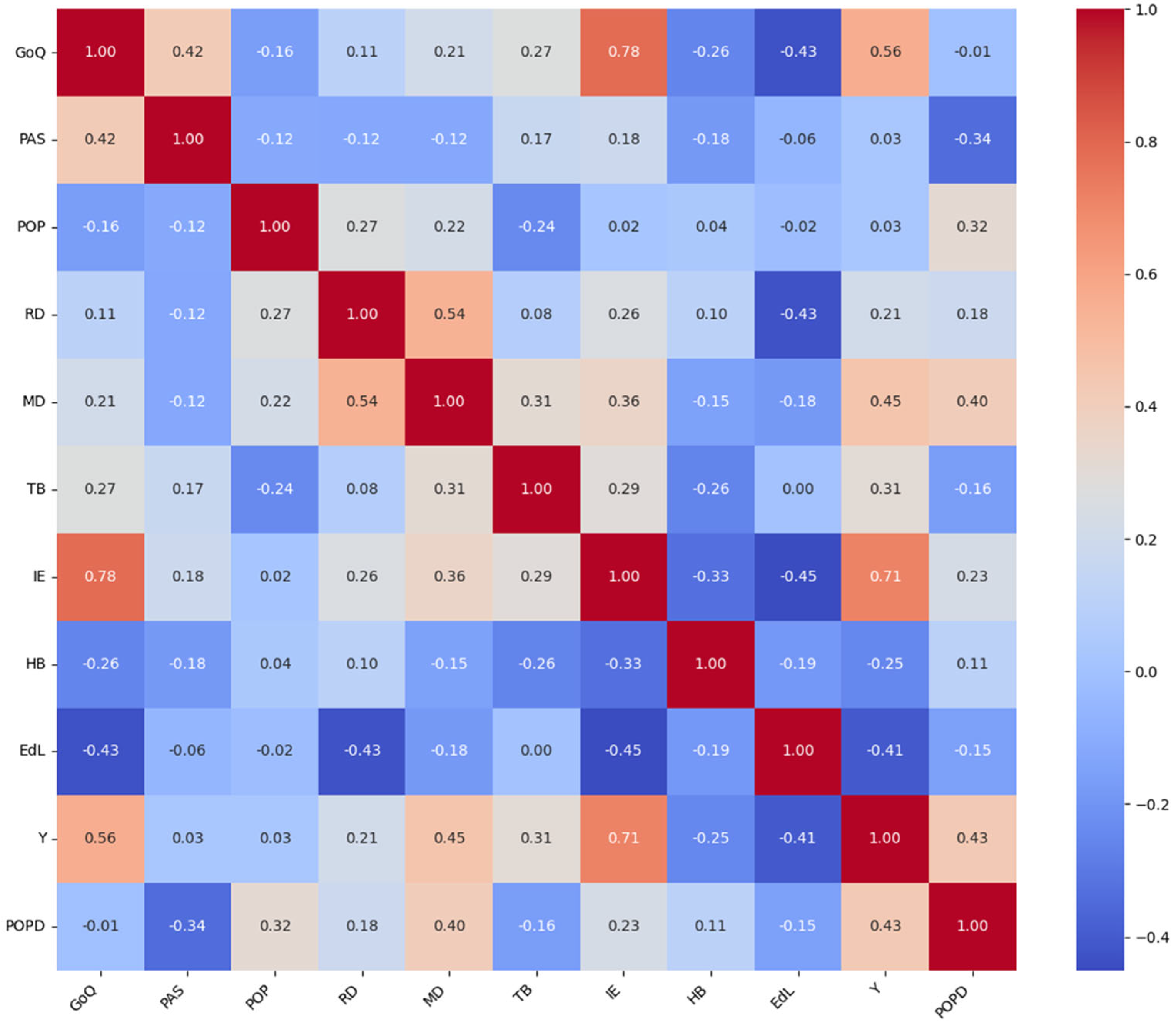
Figure 1 presents the cross-correlation between the independent variables.

3. Results

The results section is divided into four parts, starting with initial exploration of the Moran’s I findings, followed by an in-depth description of modelling for all three regional economic resilience dimensions we have used in the research.

3.1. Moran’s I

Table 3. Moran’s I on OLS residuals.

Types of Weights (W)		Resistance (Rsis)		Recovery (Rcov)		Reorientation (Rori)
		Moran’s I	p-Value	Moran’s I	p-Value	Moran’s I	p-Value
Contiguity-based	Rook	−0.0658	0.16	0.03	0.268	−0.1176	0.03
	Queen	−0.0669	0.154	0.028	0.258	−0.1226	0.026
Distance-based	200 km	−0.1462	0.003	0.0471	0.129	−0.0856	0.079
	500 km	0.0169	0.181	0.0275	0.1	−0.0134	0.394
	1000 km	−0.0077	0.494	−0.0064	0.459	−0.0141	0.253
k-nearest neighbours	1	−0.0968	0.161	0.0577	0.241	−0.0444	0.336
	2	−0.0343	0.371	0.1267	0.026	−0.0247	0.403
	3	−0.0252	0.381	0.0713	0.092	−0.041	0.277
	4	−0.0074	0.493	0.0763	0.038	0.0047	0.391
	5	−0.0302	0.27	0.0757	0.043	−0.0063	0.455
	6	−0.007	0.452	0.0704	0.037	−0.0053	0.462
	7	−0.0045	0.469	0.0549	0.051	−0.0009	0.423
	8	−0.0041	0.429	0.0437	0.097	0.0236	0.203
	9	0.0155	0.233	0.0547	0.043	0.0153	0.247
	10	0.0148	0.208	0.0485	0.046	0.0369	0.117
	11	0.0126	0.254	0.0459	0.054	0.0321	0.117
	12	0.0228	0.134	0.047	0.037	0.019	0.173
	13	0.0106	0.223	0.0481	0.04	0.0243	0.121
	14	0.0222	0.125	0.0398	0.047	0.0241	0.117
	15	0.0198	0.143	0.0424	0.03	0.0286	0.094
	16	0.0188	0.123	0.0503	0.017	0.0238	0.116
	17	0.0117	0.198	0.0542	0.018	0.0317	0.063
	18	0.0124	0.189	0.0498	0.018	0.0341	0.048
	19	0.0091	0.209	0.0433	0.033	0.0446	0.029
	20	0.0081	0.223	0.0419	0.013	0.0385	0.032
	21	0.0091	0.207	0.0401	0.031	0.0369	0.023
	22	0.0105	0.173	0.0326	0.05	0.0337	0.034
	23	0.0103	0.164	0.0271	0.05	0.0299	0.043
	24	0.009	0.184	0.0279	0.046	0.0284	0.053

reports Moran’s I on OLS residuals e from Equation (1) for Rsis, Rcov, and Rori as dependent variables.

For resistance (Rsis), Moran’s I is mostly negative and non-significant except for distance-based W 200 km, where I is 0.1462 with p = 0.003. Thus, there is no strong evidence of residual spatial autocorrelation for resistance, except possibly under a 200 km distance threshold, which suggests possible local spatial structure. The resistance model residuals show little evidence of spatial autocorrelation, which suggests that spatial spillovers are not critical for resistance. Regional resistance outcomes seem more independent across space. A region’s economic resistance to shock does not systematically depend on neighbouring regions’ resistance. It seems that standard OLS inference is appropriate. Only at very local scales (~200 km) does slight negative spatial dependence appear, suggesting localised contrasts in resistance.

For recovery (Rcov), overall spatial autocorrelation is weak but significant under certain spatial definitions. We do not detect strong spatial autocorrelation using Rook, Queen, or distance bands, but detect statistically significant spatial clustering when defining neighbours via k-nearest neighbours, especially for k ≥ 2. Local relationships (nearest neighbours) seem more important for capturing spatial effects than broader adjacency (Rook/Queen) or large distance thresholds. Still, Moran’s I values are relatively small (~0.03–0.13), indicating modest spatial dependence (not extremely strong but still relevant). Thus, recovery processes are regionally clustered. Regional economic recovery behaviours are spatially contagious. Neighbouring regions share economic structures, labour markets, infrastructure, or policy frameworks that jointly influence recovery rates, suggesting the need for spatial econometric models. Since significant spatial autocorrelation is observed, the OLS model likely suffers from spatially correlated errors, i.e., estimates may be inefficient (standard errors biased), suggesting the need for spatial models. The findings are supported by the literature, [63] which argues that resilience is not solely determined by structural vulnerability, highlighting the importance of accounting for spatial interdependencies when analysing regional recovery.

For reorientation (Rore), we find some significant negative Moran’s I under contiguity (Rook, Queen—p-values ~0.03) and positive and significant Moran’s I when many neighbours are considered (k > 17), i.e., at 18–24 neighbours (p-values < 0.05). This suggests that reorientation residuals are spatially structured, particularly at larger spatial scales (when regions are connected to 18–24 neighbours), indicating long-range spatial dependence. Thus, reorientation is spatially more fragmented locally but similar at broad scales, i.e., heterogeneity at small scales and homogeneity at larger scales. Regions near each other may take different paths (i.e., different specialisations and industries); however, across Europe, there are broader geographic zones where similar strategies emerge (i.e., southern regions reorienting toward tourism, northern regions toward high-tech).

3.2. Resistance

We estimated OLS and four types of spatial models using the resistance sensitivity index (SI_Rsis) as the dependent variable. Although Moran’s I initially suggested that a distance-weighted matrix of 200 km was most suitable, after evaluating all models across each weighting alternative (4 model types × 29 weighting alternatives), we found that the Rock and Queen contiguity matrices yielded superior results, indicated by the lowest AIC and BIC values across all models. Additionally, using the Rock and Queen contiguity matrices increased the available sample size to 143 observations, compared to 120 when using the 200 km distance-weighted matrix. The Rock and Queen contiguity matrices, however, do not capture local spatial relationships as well as the 200 km distance-weighted matrix.

Table 4. Spatial models (with Rock contiguity) and OLS estimates for regional economic resistance. Dependent variable—SI_Rsis.

Variable		OLS	SEM	SLX	SDEM	SDM
β	CONSTANT	−100.794 *	−196.529 ***	−377.709 ***	−378.748 ***	−166.720 ***
		(56.611)	(55.705)	(107.853)	(82.843)	(61.622)
	GoQ	−0.8005	−2.509	4.318	3.515	−1.719
		(1.689)	(1.885)	(3.459)	(3.294)	(2.120)
	PAS	−0.0197	0.343 ***	0.565 **	0.536 **	0.357 **
		(0.169)	(0.114)	(0.274)	(0.254)	(0.138)
	ln(POP)	1.7485	−0.946	0.658	0.575	0.048
		(1.513)	(1.493)	(1.719)	(1.599)	(1.571)
	ln(RD)	0.9755	1.683	−2.832	−1.909	1.612
		(1.729)	(2.874)	(4.037)	(3.850)	(3.154)
	ln(MD)	−1.9915	−2.968 ***	−3.072 ***	−3.015 ***	−3.039 ***
		(1.326)	(0.570)	(0.620)	(0.583)	(0.603)
	ln(TB)	2.0448	−0.712	−1.498	−1.337	−1.131
		(1.503)	(1.328)	(1.779)	(1.674)	(1.464)
	IE	−0.0742	−0.354	−0.197	−0.190	−0.444
		(0.324)	(0.322)	(0.416)	(0.393)	(0.356)
	ln(HB)	1.2697	2.967	−1.087	−1.043	0.446
		(2.401)	(3.167)	(4.706)	(4.526)	(3.452)
	EdL	0.8709 **	1.082 ***	0.666	0.588	0.958 ***
		(0.395)	(0.247)	(0.403)	(0.375)	(0.282)
	Ln(Y)	5.2340	19.243 ***	16.495 **	16.513 **	17.913 ***
		(4.372)	(4.822)	(6.845)	(6.540)	(5.390)
	ln(POPD)	0.7731	−0.336	0.916	0.715	−0.869
		(1.346)	(1.831)	(2.152)	(2.003)	(1.964)
γ	W (GoQ)			−15.127 ***	−13.215 ***
				(4.848)	(4.432)
	W (PAS)			−0.283	−0.264
				(0.317)	(0.285)
	W (ln(POP))			−7.521 ***	−7.222 ***
				(2.729)	(2.431)
	W (ln(RD))			−3.221	−3.263
				(7.660)	(6.846)
	W (ln(MD))			1.310	0.868
				(1.313)	(1.134)
	W (ln(TB))			−0.408	−0.102
				(2.994)	(2.732)
	W (IE)			0.663	0.578
				(0.661)	(0.581)
	W (ln(HB))			20.248 ***	19.770 ***
				(7.664)	(6.804)
	W (EdL)			1.030	1.162 **
				(0.610)	(0.534)
	W (ln(Y))			13.906	13.904
				(10.889)	(9.933)
	W (ln(POPD))			2.860	3.240
				(4.008)	(3.459)
ρ	W (SIRsis)					−0.067
						(0.109)
λ			−0.260 **		−0.286 **
			(0.119)		(0.119)
Number of Observations		172	143	143	143	143
Number of Variables		13	12	23	23	13
Degrees of Freedom		160	131	120	120	130
Pseudo R-squared/R-squared		0.165	0.2706	0.4360	0.4343	0.2843
Spatial Pseudo R-squared						0.2782
Log-Likelihood		−695.81	−564.1558	−548.098	−545.9385	−565.2015
Akaike Information Criterion (AIC)		1416	1152.312	1142.195	1137.877	1156.403
Schwarz Criterion (BIC)		1453	1187.866	1210.341	1206.023	1194.920

Note: *, **, and *** indicate significance at the 10, 5, and 1% level, respectively. SEM is estimated using an ML spatial error estimator; SLX is estimated using the OLS estimator; SDEM is estimated using an ML spatial error with an SLX-error estimator; SDM is estimated using an ML spatial lag estimator. Standard errors are presented in parentheses for SEM, SDEM, and SDM. White robust standard errors are presented in parentheses for SLX and OLS estimates.

presents the OLS and spatial model estimates for regional economic resistance based on the Rock contiguity matrix, though results obtained using the Queen contiguity matrix are very similar. Additionally,

Table A1. SDM direct and indirect results for economic resistance.

Variable	Direct	Indirect	Total
GoQ	−1.7186	0.1075	−1.6111
PAS	0.3573	−0.0223	0.3350
POP	0.0482	−0.0030	0.0451
RD	1.6119	−0.1008	1.5111
MD	−3.0394	0.1901	−2.8493
TB	−1.1310	0.0707	−1.0603
IE	−0.4444	0.0278	−0.4166
HB	0.4460	−0.0279	0.4181
EdL	0.9577	−0.0599	0.8978
Y	17.9125	−1.1203	16.7922
POPD	−0.8689	0.0543	−0.8146

in Appendix A.3 presents SDM direct and indirect results for economic resistance.

The spatial error term (λ) was significantly negative in both SEM and SDEM, indicating spatially correlated unobserved processes affecting regional resistance. Conversely, the spatial lag of resistance itself (ρ) in the SDM model was insignificant, suggesting a minimal direct spillover of regional employment resistance once observable factors and error dependencies were controlled.

Several explanatory variables demonstrated robust relationships with regional resistance. Demographic pressure, represented by the dependency ratio (PAS), emerged as a significant determinant across multiple models. Regions with higher proportions of non-working-age individuals (youth and elderly) consistently displayed increased vulnerability to employment shocks. Specifically, a one-percentage-point increase in the dependency ratio raises the resistance sensitivity index by approximately 0.357 points, indicating a clear weakening of regional resilience. This relationship underscores the economic strain imposed by demographic imbalances and aligns with the existing literature, which highlights the vulnerabilities associated with regions having a high proportion of young dependents [16].

Motorway density (MD), a consistently significant variable across spatial models, indicates that improved transport infrastructure substantially enhances regional resistance. A 1% increase in motorway density is associated with a reduction in the resistance sensitivity index (SIRsis) by approximately 0.03 points—an effect that becomes especially impactful with larger-scale infrastructure improvements. This robust result underscores the critical role of well-developed transport networks in maintaining economic stability and mobility during periods of disruption.

The role of education, measured by early leaving from education and training (EdL), was particularly important and consistent with past research [27]. Higher early school leaving rates correlate with increased sensitivity to economic shocks. Specifically, each additional percentage point of early school leaving increases the resistance sensitivity index by roughly 0.958 points, clearly indicating severe detrimental impacts on economic resilience. Educational disengagement, therefore, significantly compromises a region’s capacity to withstand economic disruptions, highlighting education (human capital) as a crucial area for policy intervention, in line with conclusions from [64].

Regional wealth, represented by GDP per capita (Y), showed a counterintuitive but consistently positive association with sensitivity. Wealthier regions experienced greater relative vulnerability, with a 1% increase in GDP per capita associated with an approximately 0.179-point increase in the sensitivity index. This suggests that richer regions were disproportionately impacted by the COVID-19 pandemic, possibly due to their higher integration into globally connected, service-oriented sectors that are particularly vulnerable to lockdown measures and shifts in demand. Existing literature observed that European metropolitan regions—typically the most developed and globally integrated—were more vulnerable to economic crises than rural areas [65,66]. These insights reinforce the idea that development and resilience do not always align, particularly under globally disruptive conditions.

Although not directly significant locally, hospital bed availability (HB) demonstrated important spatial spillover effects. Regions benefited significantly from increased healthcare capacity in neighbouring areas: a 1% increase in neighbouring regions’ hospital beds resulted in a roughly 0.198-point improvement in regional resistance. This finding highlights healthcare infrastructure as a crucial regional public good, with broad protective effects that transcend administrative boundaries, strengthening regional systems collectively during public health crises.

Similarly, governance quality exhibited significant positive spatial spillovers. While local governance quality was not directly linked to regional resistance, improvements in neighbouring regions significantly enhanced local resilience, reducing the sensitivity index by approximately 13.2 points. This suggests that institutional quality functions as a regional public good, producing benefits beyond administrative borders. However, this finding contrasts with [14], who found no positive—and sometimes negative—spillover effects of governance on economic growth, particularly in peripheral regions. They argue that institutional effects are often jurisdiction-bound, with well-governed regions potentially drawing resources from their neighbours. This divergence may stem from differences in timespan and resilience dimensions. In our case, governance quality is significant only for the resistance phase—not recovery or reorientation—suggesting its importance in the immediate response to shocks. In such crisis contexts, policy diffusion and cross-border cooperation may generate short-term spillovers that are less apparent in long-term growth-oriented models.

3.3. Recovery

Table 5. OLS and spatial models estimates for regional economic recovery. Dependent variable—SI_Rcov.

Variable		OLS	SEM	SLX	SDEM	SDM
β	CONSTANT	5.2630 **	5.87192 **	9.6867 *	9.78544 ***	5.8024 **
		(2.231)	(2.52624)	(5.2850)	(3.71709)	(2.4559)
	GoQ	−0.1600 **	−0.13775	−0.1384	−0.13987	−0.1237
		(0.068)	(0.08578)	(0.1352)	(0.11733)	(0.0828)
	PAS	−0.0024	−0.00162	−0.0180	−0.01753 *	−0.0009
		(0.005)	(0.00568)	(0.0114)	(0.00987)	(0.0053)
	ln(POP)	0.0024	−0.01486	−0.0627	−0.05913	−0.0079
		(0.063)	(0.06244)	(0.0781)	(0.06587)	(0.0613)
	ln(RD)	−0.0760 ***	−0.07933 **	−0.0720 *	−0.07130 **	−0.0760 **
		(0.030)	(0.03230)	(0.0366)	(0.03543)	(0.0319)
	ln(MD)	0.0278	0.02995	0.0359 *	0.03459	0.0297
		(0.018)	(0.02242)	(0.0189)	(0.02204)	(0.0223)
	ln(TB)	0.0975 *	0.10421 *	0.0696	0.06906	0.0968 *
		(0.053)	(0.05805)	(0.0885)	(0.06386)	(0.0564)
	IE	−0.0023	0.00414	−0.0076	−0.00798	0.0052
		(0.012)	(0.01423)	(0.0157)	(0.01458)	(0.0139)
	ln(HB)	−0.2316 **	−0.20762	−0.0621	−0.06496	−0.2216 *
		(0.112)	(0.13541)	(0.1845)	(0.16171)	(0.1301)
	EdL	0.0050	0.01185	0.0049	0.00492	0.0097
		(0.010)	(0.01060)	(0.0147)	(0.01299)	(0.0102)
	Ln(Y)	−0.2768	−0.41557 *	−0.5837 **	−0.57954 **	−0.4322 **
		(0.179)	(0.22334)	(0.2414)	(0.23217)	(0.2169)
	ln(POPD)	0.0204	0.05515	0.0597	0.06119	0.0512
		(0.046)	(0.06498)	(0.0567)	(0.06712)	(0.0634)
γ	W (GoQ)			0.0191	0.02810
				(0.1546)	(0.13574)
	W (PAS)			0.0242 **	0.02359 **
				(0.0115)	(0.01146)
	W (ln(POP))			0.1319	0.13247 *
				(0.0860)	(0.07882)
	W (ln(RD))			−0.0424	−0.03851
				(0.0892)	(0.09692)
	W (ln(MD))			−0.0053	−0.00766
				(0.0316)	(0.03463)
	W (ln(TB))			−0.0130	−0.00248
				(0.1143)	(0.09005)
	W (IE)			0.0153	0.01543
				(0.0194)	(0.02136)
	W (ln(HB))			−0.5244 **	−0.52907 ***
				(0.2232)	(0.19607)
	W (EdL)			−0.0126	−0.01247
				(0.0176)	(0.01820)
	W (ln(Y))			−0.1190	−0.14191
				(0.3458)	(0.31566)
	W (ln(POPD))			0.0021	0.00568
				(0.0896)	(0.09027)
ρ	W (SIRcov)					0.1159
						(0.0870)
λ			0.10354		0.04750
			(0.09139)		(0.09270)
Number of Observations		172	142	142	142	142
Number of Variables		12	12	23	23	13
Degrees of Freedom		160	130	119	119	129
Pseudo R-squared/R-squared		0.2620	0.2728	0.3865	0.3864	0.2852
Spatial Pseudo R-squared				0.2731		0.2784
Log-likelihood		−124.4600	−102.8396	−91.342	−91.2358	−102.4931
Akaike Information Criterion (AIC)		272.9000	229.679	228.684	228.472	230.986
Schwarz Criterion (BIC)		310.7000	265.149	296.668	296.456	269.412

Note: *, **, and *** indicate significance at the 10, 5, and 1% level, respectively. SEM is estimated using an ML spatial error estimator; SLX is estimated using the OLS estimator; SDEM is estimated using an ML spatial error with an SLX-error estimator; SDM is estimated using an ML spatial lag estimator. Standard errors are presented in parentheses for SEM, SDEM, and SDM. White robust standard errors are presented in parentheses for SLX and OLS estimates.

reports OLS and four types of spatial models for regional economic recovery using k-nearest neighbour weights, as previously found to be most promising in detecting possible local spatial structure. We chose k-nn = 2 because it yielded the smallest Moran’s I p-value up to k-nn = 16. Additionally,

Table A2. SDM direct and indirect results for economic recovery.

Variable	Direct	Indirect	Total
GoQ	−0.1237	−0.0162	−0.1400
PAS	−0.0009	−0.0001	−0.0010
POP	−0.0078	−0.0010	−0.0089
RD	−0.0760	−0.0100	−0.0860
MD	0.0297	0.0039	0.0335
TB	0.0968	0.0127	0.1094
IE	0.0052	0.0007	0.0059
HB	−0.2216	−0.0290	−0.2506
EdL	0.0097	0.0013	0.0110
Y	−0.4322	−0.0566	−0.4888
POPD	0.0512	0.0067	0.0580

in Appendix A.3 presents SDM’s direct and indirect results for economic recovery.

A significant finding emerges with railway density (RD), which is consistently negative and significant across SEM, SLX, SDEM, and SDM estimations. The negative coefficient, ranging closely between −0.071 and −0.079, indicates that, contrary to conventional economic intuition, regions with higher railway infrastructure density experienced slower post-crisis employment recovery compared to the EU average. A 1% increase in railway density typically reduces the sensitivity index by about 0.07 to 0.08%, a robust and consistent result. This suggests that highly developed transportation infrastructure may correspond to urbanised or industrialised areas, which are particularly vulnerable to disruptions. Perhaps these economically dense regions faced deeper initial economic shocks due to their interconnectedness and reliance on mobility, making them slower to rebound relative to less infrastructurally dense areas. This finding partially contrasts with prior research on recovery from the Great Recession in U.S. metropolitan areas, where access to local labour markets was positively associated with recovery capacity [6]. This divergence likely stems from differences in the crisis context (COVID-19 vs. 2008 recession). While road accessibility may enhance short-term labour and goods mobility, railway infrastructure often reflects structural industrial concentration, which may heighten vulnerability during globally disruptive events. This underscores the importance of differentiating between types of infrastructure and considering context-specific crisis dynamics when evaluating regional recovery performance.

The healthcare infrastructure, proxied by hospital bed (HB) availability, also offers complex insights. While HB shows a significantly negative direct coefficient in SDM (−0.2216), indicating regions with higher healthcare capacities seemingly recovered more slowly, a paradoxical interpretation emerges when accounting explicitly for spatial spillovers. Spatial lagged estimations in SLX and SDEM notably show strongly negative spatial coefficients (−0.5244 and −0.5291, respectively). This implies that regions surrounded by neighbours with extensive healthcare capacities might experience resource competition or stricter public health policies that constrain regional economic activity during crises, thereby hindering their relative economic recovery. Nevertheless, SDM impacts clarify this paradox: direct effects are positive (0.4460), implying that robust local healthcare infrastructure significantly boosts regional economic resilience; simultaneously, indirect spatial effects remain negative yet minor (−0.0279). This indicates that, while healthcare infrastructure significantly enhances local resilience, reflecting better health outcomes, lower pandemic-related disruptions, and improved long-term economic attractiveness, it can induce small competitive effects on neighbouring regions, likely due to uneven resource distribution or regional competition for public health resources during crises.

Regional economic wealth, measured by GDP per capita (Y), presents another compelling result. Across SEM, SLX, SDEM, and SDM, GDP per capita consistently shows a significant negative coefficient, ranging notably between −0.4156 and −0.5837. Superficially, this result might seem counterintuitive, suggesting richer regions recover relatively more slowly. Yet, wealthier regions may initially suffer larger absolute economic shocks due to greater economic complexity and international exposure, thus appearing to recover more slowly when compared strictly relative to the EU average, particularly in the context of a pandemic-induced crisis. This pattern aligns with our earlier findings for the resistance dimension and is consistent with insights from the existing literature [66].

A notably richer interpretation emerges when spatial interactions are explicitly considered in the SDM impacts: the direct effect of GDP per capita becomes highly positive (17.9125), highlighting unequivocally that wealthier regions have robust local economic resilience stemming from greater diversification, superior human capital, and institutional advantages. Nevertheless, spatial spillovers are negative (−1.1203), possibly reflecting that affluent regions attract resources, investments, or skilled labour from neighbouring areas, potentially dampening their neighbours’ recoveries. The total effect remains strongly positive (16.7922), confirming the overall substantial economic resilience benefits of regional prosperity once spatial dynamics are comprehensively accounted for. This aligns with the view of [67], who suggests that, while national-level economic strength can aid recovery, aspects such as local adaptability and regional governance remain crucial in shaping resilience outcomes.

Regarding the demographic structures captured by the dependency ratio (PAS)—the share of youth and elderly relative to the working-age population—a nuanced spatial interpretation emerges. The SDEM model shows PAS as negatively significant (−0.0175), indicating that regions with higher demographic burdens (more dependent populations) recover more slowly. This aligns with expectations [16] because higher dependency ratios typically strain social welfare systems, reduce labour market flexibility, and dampen innovation. However, spatial lagged effects are significantly positive (0.0236–0.0242 in SLX and SDEM), suggesting that regions may benefit from proximity to neighbours with higher dependency burdens. This positive spillover may arise because regions with more balanced demographic structures might attract labour and investments away from neighbouring areas burdened by demographic pressures, thus boosting their own resilience. The SDM model further clarifies this picture, demonstrating significant direct positive effects (0.3573) alongside slight adverse indirect effects (−0.0223). This signifies that, while balanced demographics locally strengthen regional economic resilience, neighbouring regions’ demographic pressures create minor competitive dynamics. Hence, demographic structure’s resilience implications critically hinge on both local labour market flexibility and interregional migratory and resource dynamics.

Spatial autocorrelation parameters (ρ and λ) remain insignificant, indicating limited unexplained spatial correlation. This suggests that the models adequately control for critical spatial interactions and region-specific heterogeneities affecting economic resilience.

Finally, reflecting upon OLS results, it is evident that ignoring spatial dynamics significantly understates and misinterprets regional resilience factors. OLS estimations appear weaker and less reliable and fail to capture the complex interdependencies and spillovers effectively elucidated by the spatial models. Therefore, spatial econometric approaches provide superior insights into the determinants of regional economic recovery.

In summary, regional resilience dynamics depend on infrastructure density, healthcare capacities, regional economic wealth, and demographic structures. Each demonstrates significant local effects, tempered by spatial spillovers that underscore competitive or resource redistribution pressures. Policymakers aiming to enhance regional resilience must thus acknowledge these spatial interdependencies, designing policies that balance local benefits with broader regional cohesion and equity to optimise overall economic recovery outcomes.

3.4. Reorientation

Table 6. OLS and spatial models estimates for regional economic reorientation. Dependent variable—SI_Rori.

Variable		OLS	SEM	SLX	SDEM	SDM
β	CONSTANT	15.9158	25.13995 **	23.11372	18.26924	25.85145 *
		(12.357)	(11.68590)	(23.46833)	(18.46501)	(13.52230)
	GoQ	0.3962	0.56957	−0.43176	−0.18333	0.57153
		(0.386)	(0.39687)	(0.79284)	(0.75473)	(0.46391)
	PAS	−0.0522	−0.04684 **	0.00490	−0.00146	−0.05828 *
		(0.032)	(0.02354)	(0.06226)	(0.06081)	(0.03075)
	ln(POP)	−0.7282 **	−0.87790 ***	−0.92011 *	−0.97317 **	−0.81451 **
		(0.336)	(0.32024)	(0.48254)	(0.38524)	(0.35177)
	ln(RD)	0.3853 ***	−1.79502 ***	−0.27817	−0.11789	−1.90685 ***
		(0.147)	(0.60252)	(0.98902)	(0.90158)	(0.68686)
	ln(MD)	−0.2458 *	−0.16550	−0.00955	0.00406	−0.14112
		(0.143)	(0.12667)	(0.15854)	(0.14043)	(0.13735)
	ln(TB)	0.9123 **	0.22447	1.29512 ***	1.28262 ***	0.50473
		(0.390)	(0.28131)	(0.45926)	(0.39545)	(0.32236)
	IE	−0.0318	−0.01335	−0.09979	−0.08792	−0.03271
		(0.062)	(0.06802)	(0.09372)	(0.09723)	(0.07941)
	ln(HB)	−0.8168	−0.51246	−1.25241	−1.29714	−0.56365
		(0.603)	(0.66795)	(0.93638)	(1.04315)	(0.75716)
	EdL	0.1519 *	0.08609 *	0.04747	0.05595	0.10117
		(0.089)	(0.05187)	(0.10744)	(0.08575)	(0.06198)
	Ln(Y)	0.0433	0.25110	0.05294	−0.13130	0.20084
		(0.951)	(1.01188)	(1.58372)	(1.54420)	(1.18474)
	ln(POPD)	−0.2087	0.24225	0.10701	0.19054	0.33716
		(0.275)	(0.38652)	(0.62192)	(0.46053)	(0.42651)
γ	W (GoQ)			0.0191	0.02810
				(0.1546)	(0.13574)
	W (PAS)			0.0242 **	0.02359 **
				(0.0115)	(0.01146)
	W (ln(POP))			0.1319	0.13247 *
				(0.0860)	(0.07882)
	W (ln(RD))			−0.0424	−0.03851
				(0.0892)	(0.09692)
	W (ln(MD))			−0.0053	−0.00766
				(0.0316)	(0.03463)
	W (ln(TB))			−0.0130	−0.00248
				(0.1143)	(0.09005)
	W (IE)			0.0153	0.01543
				(0.0194)	(0.02136)
	W (ln(HB))			−0.5244 **	−0.52907 ***
				(0.2232)	(0.19607)
	W (EdL)			−0.0126	−0.01247
				(0.0176)	(0.01820)
	W (ln(Y))			−0.1190	−0.14191
				(0.3458)	(0.31566)
	W (ln(POPD))			0.0021	0.00568
				(0.0896)	(0.09027)
ρ	W (SIRcov)					−0.26258 **
						(0.11512)
λ			−0.38110 ***		−0.30646 **
			(0.12023)		(0.12099)
Number of Observations		164	138	138	138	138
Number of Variables		12	12	23	23	13
Degrees of Freedom		152	126	115	115	125
Pseudo R-squared/R-squared		0.218	0.1731	0.3221	0.3186	0.2266
Spatial Pseudo R-squared				0.2731		0.1761
Log-likelihood		−401.25	−333.7319	−324.715	−322.0503	−334.9257
Akaike Information Criterion (AIC)		826.5	691.464	695.430	690.101	695.851
Schwarz Criterion (BIC)		863.7	726.591	762.757	757.427	733.906

Note: *, **, and *** indicate significance at the 10, 5, and 1% level, respectively. SEM is estimated using an ML spatial error estimator; SLX is estimated using the OLS estimator; SDEM is estimated using an ML spatial error with an SLX-error estimator; SDM is estimated using an ML spatial lag estimator. Standard errors are presented in parentheses for SEM, SDEM, and SDM. White robust standard errors are presented in parentheses for SLX and OLS estimates.

reports OLS and four types of spatial models for regional economic reorientation (Rori) using the Queen contiguity matrix, as previously found to be most promising in detecting possible local spatial structure, though results obtained using the Rock contiguity matrix are very similar. Additionally,

Table A3. SDM direct and indirect results for economic reorientation.

Variable	Direct	Indirect	Total
GoQ	0.5715	−0.1189	0.4527
PAS	−0.0583	0.0121	−0.0462
POP	−0.8145	0.1694	−0.6451
RD	−1.9068	0.3966	−1.5103
MD	−0.1411	0.0293	−0.1118
TB	0.5047	−0.1050	0.3998
IE	−0.0327	0.0068	−0.0259
HB	−0.5636	0.1172	−0.4464
EdL	0.1012	−0.0210	0.0801
Y	0.2008	−0.0418	0.1591
POPD	0.3372	−0.0701	0.2670

in Appendix A.3 presents SDM direct and indirect results for economic reorientation.

Population structure, specifically the dependency ratio (PAS), emerged as a significant determinant of regional economic resilience across multiple spatial models, notably in SEM and SDM. SEM reveals that an increase in the dependency ratio significantly decreases regional resilience (β = −0.0468, significant at the 5% level), a finding similarly observed in the direct effects from SDM (β = −0.0583, significant at the 10% level). This implies that regions burdened with relatively larger young and elderly populations face considerable challenges in adapting their economies toward high-tech employment. Such demographic structures constrain labour market flexibility, strain public resources (particularly healthcare and education systems), and, ultimately, hinder innovation and economic adaptation. Interestingly, a subtle positive spatial spillover of dependency ratios in neighbouring regions (γ ≈ 0.024, significant in SLX and SDEM) suggests minor beneficial inter-regional effects, possibly driven by the migration of young workers or shared cross-border public service efficiencies. In broader terms, these findings indicate the critical role of demographics in regional adaptability.

Population size (POP) consistently appears as a significant negative factor in regional resilience across all spatial econometric specifications—SEM, SLX, SDEM, and SDM—with effect sizes ranging roughly between −0.81 and −0.97, statistically significant at various levels (from 1% to 10%). This counterintuitive outcome highlights that regions with larger populations are often slower in economic reorientation towards high-tech sectors, potentially due to inherent socioeconomic complexities, institutional inertia, and difficulties in rapidly transforming established economic structures. Despite the potential advantages of economies of scale, large regions may become less agile and adaptive, particularly under sudden economic shocks; however, the indirect spatial effect in SDM (γ = 0.13247, significant at the 10% level) also suggests that proximity to larger regions might confer modest resilience benefits through knowledge spillovers or agglomeration effects. These findings underline a delicate balance: while large regional populations provide market scale and political leverage, they pose significant challenges to swift economic restructuring.

Railway infrastructure density (RD) negatively correlates with regional economic resilience reorientation, exhibiting strongly negative and statistically significant impacts in both SEM (β = −1.7950, significant at 1%) and SDM (β = −1.9069, significant at 1%). Contrary to expectations, denser railway networks appear to be linked with economic rigidity, possibly reflecting regional economic legacies characterised by heavy industry, older manufacturing bases, or outdated infrastructure focused on declining sectors. Such infrastructural rigidity may limit regions’ ability to pivot effectively toward innovation-intensive sectors during economic disruptions. The magnitude of this negative impact indicates substantial constraints on economic adaptability due to historical infrastructural patterns.

In contrast, tourism infrastructure—measured by tourism bed capacity (TB)—emerges as a robust and positive determinant of regional adaptive resilience, particularly in SLX and SDEM (β ≈ 1.29, significant at the 1% level). While the current literature [66] presents mixed findings on the impact of inbound and outbound tourism on resilience, our novel results, framed through the lens of evolutionary resilience, can be interpreted in two complementary ways. The first, more straightforward interpretation is that well-developed tourism infrastructure reflects a diversified and service-oriented economic base, which is better equipped to adapt effectively during periods of economic transition. A strong tourism sector may not only create employment opportunities but also contribute to broader economic maturity, stimulate local business development, and enhance a region’s capacity for innovation. Alternatively, given the specific nature of the crisis examined—namely, the COVID-19 pandemic—regions with a high dependence on tourism may have experienced disproportionately severe impacts and, as a result, were compelled to undergo rapid transformation. This may have involved reallocating resources toward more resilient, technology-intensive sectors as a survival strategy. In both scenarios, regions with greater tourism capacity appear to exhibit superior adaptability and a stronger capacity to shift toward new economic pathways.

Spatial interactions regarding healthcare infrastructure (HB) reveal negative spillover effects. Indirect spatial effects (in SLX and SDEM) indicate that proximity to regions with extensive healthcare infrastructure significantly reduces local economic resilience (γ ≈ −0.52, significant at 1–5%). This suggests inter-regional competitive dynamics, possibly reflecting the capacity of stronger healthcare regions to attract skilled human capital, resources, and investments, thereby inadvertently weakening neighbouring regions’ adaptability. Regarding spatial dependence parameters, the spatial autoregressive parameter (ρ) in SDM (−0.26258, significant at 5%) indicates significant negative spatial autocorrelation, highlighting competitive rather than cooperative relationships among neighbouring regions. Thus, economic improvements in one region may come at the expense of neighbouring regions, underscoring competitive regional dynamics. Similarly, the significant negative spatial error terms (λ = −0.3811 in SEM, significant at 1%; λ = −0.3065 in SDEM, significant at 5%) confirm negative spillovers from unobserved regional shocks, implying interconnected regional vulnerabilities. This supports the notion that post-crisis adaptive resilience is strongly influenced by region-specific factors, aligning with [68], who highlights the importance of regional effects in shaping growth trajectory aftershocks.

OLS estimations reveal that, while results are broadly consistent in significance and directionality with spatial models for variables such as population size, railway density, and tourism infrastructure, the OLS method inherently ignores spatial effects and inter-regional dynamics, thereby providing incomplete insights into regional resilience.

4. Discussion and Policy Implications

The empirical findings from our spatial econometric analyses provide insights into how different types of infrastructure influence regional economic resilience across resistance, recovery, and reorientation dimensions. Methodologically, this study contributes to the literature by systematically applying 29 spatial weighting matrices across four spatial models, enabling a robust and comprehensive analysis of spatial dependencies that are often overlooked in resilience research. Additionally, our use of a sensitivity index and a novel high-tech employment-based reorientation measure ensures consistent and comparable resilience dimensions, enabling comprehensive cross-dimensional analysis. Theoretically, this research advances understanding of the multifaceted role of infrastructure within regional economic resilience, particularly in the underexplored context of the COVID-19 pandemic. These results hold significant implications for policymakers aiming to enhance regional stability and adaptive capacity through targeted infrastructure investments and spatially informed development strategies.

4.1. Implications to Enhance Resistance

Our analysis underscores that targeted infrastructure investments should remain foundational to regional resilience strategies, particularly in transport infrastructure and educational systems, given their primarily localised benefits. For instance, motorway density emerged as a statistically robust predictor of lower economic vulnerability, supporting its role not just as a facilitator of growth but as an early indicator of resilience. This finding strengthens the case for pre-emptive transport infrastructure investment in resilience planning.

Demographic structures also significantly influence regional resistance, as regions with higher demographic dependency ratios—dominated by non-working-age populations—demonstrate increased vulnerability. Policymakers should, therefore, actively pursue demographic sustainability measures targeted demographic policies (e.g., family support, active ageing, balanced migration) as part of regional resilience strategies.

Healthcare infrastructure, while not directly significant locally, presented crucial positive spatial spillovers. Regions significantly benefited from robust healthcare systems in neighbouring areas, emphasising that regional healthcare infrastructure is a public good. Thus, policymakers should view healthcare enhancements strategically as regional rather than purely local initiatives, capitalising on collaborative and coordinated healthcare planning across regional boundaries.

Governance quality revealed significant spatial spillover benefits, demonstrating that improving institutional quality in adjacent regions considerably strengthens local resilience. This supports the view of [63] that good governance is a critical component of resilience; hence, regional economic policies must prioritise cross-regional governance improvements, recognising that strong governance institutions have substantial externalities that bolster economic stability.

4.2. Implications to Boost Recovery

Transportation infrastructure, specifically railway density, revealed complex spatial dynamics during regional recovery phases. Although denser railway networks positively enhance local resilience, they simultaneously impose competitive pressures and resource allocation challenges on neighbouring regions. This duality highlights a novel insight: infrastructure resilience is not inherently symmetric across space. Policymakers must therefore shift from isolated upgrades toward spatially coordinated transport strategies, ensuring that investments enhance regional resilience without inadvertently creating disparities.

Healthcare infrastructure demonstrated similarly asymmetric effects. Robust local healthcare capacity improved regional recovery, yet the concentration of such infrastructure in a few regions resulted in competitive spatial externalities, disadvantaging surrounding areas. These findings emphasise the need for integrated, cross-regional healthcare planning, particularly in crisis-prone contexts, so that healthcare systems act as stabilisers, not sources of regional imbalance.

The direct positive influence of regional economic prosperity on recovery underscores the importance of diversified economic development strategies. Nonetheless, affluent regions risk inadvertently exacerbating inequalities through negative spillovers by drawing resources and opportunities from less prosperous neighbours. Policymakers must address this by fostering inclusive regional development initiatives, resource-sharing agreements, and coordinated investments to ensure benefits extend across broader economic clusters or corridors.

4.3. Implications to Promote Reorientation

While reorientation remains the least explored dimension of regional resilience in empirical research, particularly in relation to infrastructure, our findings offer novel insights into this adaptive phase. Policymakers should prioritise strategies that enhance demographic sustainability and labour market flexibility, as regions with higher dependency ratios consistently exhibit weaker capacities to reorient toward high-tech or knowledge-based activities. Targeted interventions, such as youth integration into innovation sectors and expanded support for elder care, can strengthen demographic foundations for long-term adaptability.

Our analysis reveals that regions with dense railway infrastructure experienced greater economic rigidity, suggesting that existing infrastructural patterns sometimes impede necessary economic transitions. Consequently, policymakers should promote infrastructure flexibility, including multimodal transportation networks, to support diversified, innovation-driven economic activities and to avoid entrenched economic dependencies.

Tourism infrastructure appears to significantly enhance regional adaptability. Strategic investment in high-quality tourism infrastructure should be viewed not only as a driver of direct economic activity but also as a foundation for broader economic diversification and resilience. Regions with strong tourism sectors may be better positioned to absorb and adapt to shocks, as seen during the COVID-19 crisis. Notably, even though tourism-dependent regions were among the most severely impacted, many demonstrated a remarkable capacity for structural transformation, redirecting resources toward more resilient and innovation-driven sectors such as high-tech services and the digital economy. This suggests that a well-developed tourism infrastructure can serve as a platform for economic flexibility and renewal. Policymakers should, therefore, consider tourism not just as a traditional service sector, but as a strategic asset that, when supported by complementary policies, can contribute to long-term regional resilience and adaptive capacity in the face of future disruptions.

Finally, healthcare infrastructure revealed spatially uneven effects, reinforcing the need for regional coordination. Without collaborative planning, the concentration of health resources may exacerbate disparities, limiting vulnerable regions’ ability to reorient effectively. Cross-border healthcare strategies can help to equalize adaptive capacity and ensure health systems support, rather than fragment, regional transitions.

4.4. Research Limitations

This research focuses primarily on the COVID-19 crisis period. The policy implications are framed with this context in mind; however, crises rarely occur in isolation. During the same period, overlapping shocks, such as the Russo-Ukrainian war, disruptions in global supply chains, and the energy crisis, also took place. The broader economic environment was marked by rising inflation, which is not accounted for in this study. Future research should explore more deeply how interconnected and compounding crises affect regional economic resilience.

An important methodological consideration in our study is the choice of reference level for calculating sensitivity indices. Given the EU-wide scope of our analysis, we opted to use the EU27 average rather than national averages. This decision was driven by three key factors: (1) the need for a common benchmark to ensure comparability across all NUTS-2 regions, regardless of national affiliation; (2) the presence of countries with only a single NUTS-2 region (e.g., Estonia), where national and regional values are identical and thus analytically uninformative; and (3) the use of spatial econometric models involving cross-border spatial interactions, which would be methodologically inconsistent with nationally bounded sensitivity benchmarks. While we believe this EU-level reference provides a more coherent and spatially appropriate approach for cross-country resilience analysis, we also recognise that the national level remains the most suitable reference when investigating regional resilience within a single country. Future research could explore how sensitivity indices and spatial spillovers, particularly under specific spatial weighting schemes, behave within national- or country-group-level models, especially when comparing resilience patterns across different types of crises within individual member states.

Using motorway and railway density may underrepresent connectivity in island regions, whereas alternatives such as seaports or airports would limit coverage in inland areas. This trade-off presents a challenge in Europe-wide spatial studies, which utilise various spatial matrices and is an area that future research could address. In addition, relying solely on hospital bed availability as a proxy for healthcare infrastructure may overlook critical aspects of crisis response capacity, such as ICU availability. Future research could incorporate both metrics to better capture regional resistance and recovery, particularly during health-driven economic shocks such as the COVID-19 pandemic. Finally, we recognise the importance of considering alternative or multidimensional metrics to measure regional economic resilience instead of relying solely on employment sensitivity, and we encourage researchers to explore this area more thoroughly in the future.

This research focuses on traditional infrastructure dimensions, such as transport and healthcare, without explicitly incorporating the emerging role of digital and smart infrastructure, often referred to as Infrastructure 4.0. This includes the integration of AI and digital finance systems, which are increasingly shaping regional connectivity and economic resilience. Recent studies demonstrate spatial clustering and positive correlations between digitally inclusive finance and regional resilience [69]. At the same time, other empirical research shows that AI significantly enhances regional economic resilience by improving efficiency [70]. These findings suggest that digital infrastructure, including AI, may significantly influence regional adaptive capacities. Future research could address this limitation by incorporating measures of digital infrastructure, AI, and digital finance to capture the evolving nature of infrastructure in regional resilience analyses.

References

1. Schimmelfennig, F. Crisis and Polity Formation in the European Union. J. Eur. Public Policy 2024, 31, 3396–3420. [Google Scholar] [CrossRef] [PubMed]
2. Börzel, T.A. European Integration and the War in Ukraine: Just Another Crisis? JCMS J. Common Mark. Stud. 2023, 61, 14–30. [Google Scholar] [CrossRef]
3. Eraydin, A. Attributes and Characteristics of Regional Resilience: Defining and Measuring the Resilience of Turkish Regions. Reg. Stud. 2016, 50, 600–614. [Google Scholar] [CrossRef]
4. Meng, T.; Tian, C.; Zhang, H.; Koo, C.K. What Effects of COVID-19 on Regional Economic Resilience? Evidence from 31 Provinces in China. Front. Public Health 2022, 10, 973107. [Google Scholar] [CrossRef] [PubMed]
5. Tupy, I.S.; Silva, F.F.; Diniz, G.F.C.; Montenegro, R.L.; de Queiroz Stein, A.; Ferraz, D. Resilient Regions in Brazil: Unfolding the Effects of COVID-19 From a Socioeconomic Perspective. Int. Reg. Sci. Rev. 2023, 46, 649–677. [Google Scholar] [CrossRef]
6. Chacon-Hurtado, D.; Kumar, I.; Gkritza, K.; Fricker, J.D.; Beaulieu, L.J. The Role of Transportation Accessibility in Regional Economic Resilience. J. Transp. Geogr. 2020, 84, 102695. [Google Scholar] [CrossRef]
7. Gambe, T.R.; Geyer, H.S.; Horn, A. Economic Resilience of City-Regions in Southern Africa: An Exploratory Study of Zimbabwe. Reg. Sci. Policy Pract. 2022, 14, 438–455. [Google Scholar] [CrossRef]
8. Rimidis, M.; Butkus, M. From Adversity to Advantage: A Systematic Literature Review on Regional Economic Resilience. Urban Sci. 2025, 9, 118. [Google Scholar] [CrossRef]
9. Martin, R. Regional Economic Resilience, Hysteresis and Recessionary Shocks. J. Econ. Geogr. 2012, 12, 1–32. [Google Scholar] [CrossRef]
10. Psycharis, Y.; Panori, A.; Athanasopoulos, D. Public Investment and Regional Resilience: Empirical Evidence from the Greek Regions. Tijdschr. Voor Econ. En Soc. Geogr. 2022, 113, 57–79. [Google Scholar] [CrossRef]
11. Terzo, G. Social Capital, Social Economy and Economic Resilience of Italian Provinces. Pap. Reg. Sci. 2021, 100, 1113–1135. [Google Scholar] [CrossRef]
12. Compagnucci, F.; Gentili, A.; Valentini, E.; Gallegati, M. Asymmetric Responses to Shocks: The Role of Structural Change on Resilience of the Euro Area Regions. Appl. Econ. 2022, 54, 4324–4355. [Google Scholar] [CrossRef]
13. Ezcurra, R.; Rios, V. Quality of Government and Regional Resilience in the European Union. Evidence from the Great Recession. Pap. Reg. Sci. 2019, 98, 1267–1290. [Google Scholar] [CrossRef]
14. Annoni, P.; de Dominicis, L.; Khabirpour, N. Location Matters: A Spatial Econometric Analysis of Regional Resilience in the European Union. Growth Change 2019, 50, 824–855. [Google Scholar] [CrossRef]
15. Rocchetta, S.; Mina, A.; Lee, C.; Kogler, D.F. Technological Knowledge Spaces and the Resilience of European Regions. J. Econ. Geogr. 2022, 22, 27–51. [Google Scholar] [CrossRef]
16. Rios, V.; Gianmoena, L. The Link between Quality of Government and Regional Resilience in Europe. J. Policy Model. 2020, 42, 1064–1084. [Google Scholar] [CrossRef]
17. Pontarollo, N.; Serpieri, C. Challenges and Opportunities to Regional Renewal in the European Union. Int. Reg. Sci. Rev. 2021, 44, 142–169. [Google Scholar] [CrossRef]
18. Cainelli, G.; Ganau, R.; Modica, M. Industrial Relatedness and Regional Resilience in the European Union. Pap. Reg. Sci. 2019, 98, 755–778. [Google Scholar] [CrossRef]
19. Giannakis, E.; Bruggeman, A. Regional Disparities in Economic Resilience in the European Union across the Urban–Rural Divide. Reg. Stud. 2020, 54, 1200–1213. [Google Scholar] [CrossRef]
20. Zádor, Z.; Zhu, Z.; Smith, M.; Gorgoni, S. The Effect of Value Chain Importance on Regional Economic Recovery. Eur. Plan. Stud. 2024, 32, 843–862. [Google Scholar] [CrossRef]
21. Tsiapa, M. Social Capital and Characteristics of Economic Dualism as Determinants of Regional Resilience. Eur. Plan. Stud. 2023, 31, 2568–2589. [Google Scholar] [CrossRef]
22. Di Pietro, F.; Lecca, P.; Salotti, S. Regional Economic Resilience in the European Union: A Numerical General Equilibrium Analysis. Spat. Econ. Anal. 2021, 16, 287–312. [Google Scholar] [CrossRef]
23. Kitsos, A.; Carrascal-Incera, A.; Ortega-Argilés, R. The Role of Embeddedness on Regional Economic Resilience: Evidence from the UK. Sustainability 2019, 11, 3800. [Google Scholar] [CrossRef]
24. Faggian, A.; Gemmiti, R.; Jaquet, T.; Santini, I. Regional Economic Resilience: The Experience of the Italian Local Labor Systems. Ann. Reg. Sci. 2018, 60, 393–410. [Google Scholar] [CrossRef]
25. Martin, R.; Sunley, P. Complexity Thinking and Evolutionary Economic Geography. J. Econ. Geogr. 2007, 7, 573–601. [Google Scholar] [CrossRef]
26. Martin, R.L. Shocking Aspects of Regional Development: Towards an Economic Geography of Resilience. In The New Oxford Handbook of Economic Geography; Clark, G.L., Feldman, M., Gertler, M.S., Wójcik, D., Eds.; Oxford University Press: Oxford, UK, 2018; ISBN 978-0-19-875560-9. [Google Scholar]
27. Sutton, J.; Kobara, Y.M.; Arku, G. Determinants of Regional Economic Resilience and Post-Crisis Growth Path Performance: Insights from Canada. Reg. Stud. 2025, 59, 2429571. [Google Scholar] [CrossRef]
28. Sutton, J.; Sutton, J. A Road Map to Capture the Spatial Dependence Underlying Regions’ Economic Resilience. Spat. Econ. Anal. 2024, 19, 57–72. [Google Scholar] [CrossRef]
29. LeSage, J.P. What Regional Scientists Need to Know about Spatial Econometrics. Rev. Reg. Stud. 2014, 44, 13–32. [Google Scholar] [CrossRef]
30. Abreu, M.; de Groot, H.; Florax, R. Space and growth: A survey of empirical evidence and methods. Reg. Dev. 2005, 21, 13–44. [Google Scholar] [CrossRef]
31. Anselin, L. Spatial Models in Econometric Research. In Oxford Research Encyclopedia of Economics and Finance; Oxford University Press: Oxford, UK, 2021; ISBN 978-0-19-062597-9. [Google Scholar]
32. Liu, C.; Peng, M.Y.-P.; Gong, W. Spatial Spillover Effects Promote the Overall Improvement of Urban Competitiveness: Evidence of SDM in Asian Cities. Front. Environ. Sci. 2022, 10, 779596. [Google Scholar] [CrossRef]
33. Cainelli, G.; Ganau, R.; Modica, M. Does Related Variety Affect Regional Resilience? New Evidence from Italy. Ann. Reg. Sci. 2019, 62, 657–680. [Google Scholar] [CrossRef]
34. Giannakis, E.; Bruggeman, A.; Mamuneas, T.P. Regional Economic Resilience, Productivity Growth and Sectoral Interconnectedness. Pap. Reg. Sci. 2024, 103, 100010. [Google Scholar] [CrossRef]
35. Yildirim, V.; Mert Kantar, Y. Robust Estimation Approach for Spatial Error Model. J. Stat. Comput. Simul. 2020, 90, 1618–1638. [Google Scholar] [CrossRef]
36. Halleck Vega, S.; Elhorst, J.P. The Slx Model. J. Reg. Sci. 2015, 55, 339–363. [Google Scholar] [CrossRef]
37. Holling, C.S. Resilience and Stability of Ecological Systems. Annu. Rev. Ecol. Syst. 1973, 4, 1–23. [Google Scholar] [CrossRef]
38. Fingleton, B.; Garretsen, H.; Martin, R. Recessionary shocks and regional employment: Evidence on the resilience of U.K. regions. J. Reg. Sci. 2012, 52, 109–133. [Google Scholar] [CrossRef]
39. Martin, R.; Sunley, P. On the Notion of Regional Economic Resilience: Conceptualization and Explanation. J. Econ. Geogr. 2015, 15, 1–42. [Google Scholar] [CrossRef]
40. Simmie, J.; Martin, R. The Economic Resilience of Regions: Towards an Evolutionary Approach. Camb. J. Reg. Econ. Soc. 2010, 3, 27–43. [Google Scholar] [CrossRef]
41. Boschma, R. Towards an Evolutionary Perspective on Regional Resilience. Reg. Stud. 2015, 49, 733–751. [Google Scholar] [CrossRef]
42. Hassink, R. Regional Resilience: A Promising Concept to Explain Differences in Regional Economic Adaptability? Camb. J. Reg. Econ. Soc. 2010, 3, 45–58. [Google Scholar] [CrossRef]
43. Sensier, M.; Artis, M. The Resilience of Employment in Wales: Through Recession and into Recovery. Reg. Stud. 2016, 50, 586–599. [Google Scholar] [CrossRef]
44. Giannakis, E.; Papadas, C.T. Spatial Connectivity and Regional Economic Resilience in Turbulent Times. Sustainability 2021, 13, 1289. [Google Scholar] [CrossRef]
45. Giannakis, E.; Bruggeman, A. Determinants of Regional Resilience to Economic Crisis: A European Perspective. Eur. Plan. Stud. 2017, 25, 1394–1415. [Google Scholar] [CrossRef]
46. Wu, C.; Zhang, N.; Xu, L. Travelers on the Railway: An Economic Growth Model of the Effects of Railway Transportation Infrastructure on Consumption and Sustainable Economic Growth. Sustainability 2021, 13, 6863. [Google Scholar] [CrossRef]
47. Beyzatlar, M.A.; Kuştepeli, Y. Infrastructure, Economic Growth and Population Density in Turkey. Int. J. Econ. Sci. Appl. Res. 2011, 4, 39–57. [Google Scholar]
48. Chandra, A.; Thompson, E. Does Public Infrastructure Affect Economic Activity?: Evidence from the Rural Interstate Highway System. Reg. Sci. Urban Econ. 2000, 30, 457–490. [Google Scholar] [CrossRef]
49. Bisaschi, L.; Ceccanti, D.; Romano, F.; Calofir, L.; Carlberg, M.; Carneiro, J. Transport Infrastructure in Low-Density and Depopulating Areas: Research for TRAN Committee; Publications Office of the European Union: Luxembourg, 2021; ISBN 978-92-846-7695-8. [Google Scholar]
50. Šulc, I.; Opačić, V.T. Typology of Tourist Resorts in Croatia: The Case of South Dalmatia. Mitteilungen Osterr. Geogr. Ges. 2015, 157, 229–252. [Google Scholar] [CrossRef]
51. Mwamba, N.M.; Muhanji, S.; Kipchumba, S. Bed Occupancy as a Predictor of Tourism Performance Index in Kenya | The International Journal of Humanities & Social Studies. Int. J. Humanit. Soc. Stud. 2020, 8, 136–142. [Google Scholar] [CrossRef]
52. Ravaghi, H.; Alidoost, S.; Mannion, R.; Bélorgeot, V.D. Models and Methods for Determining the Optimal Number of Beds in Hospitals and Regions: A Systematic Scoping Review. BMC Health Serv. Res. 2020, 20, 186. [Google Scholar] [CrossRef]
53. Grimes, S. How Well Are Europe’s Rural Businesses Connected to the Digital Economy? Eur. Plan. Stud. 2005, 13, 1063–1081. [Google Scholar] [CrossRef]
54. Salemink, K.; Strijker, D.; Bosworth, G. Rural Development in the Digital Age: A Systematic Literature Review on Unequal ICT Availability, Adoption, and Use in Rural Areas. J. Rural. Stud. 2017, 54, 360–371. [Google Scholar] [CrossRef]
55. Hota, S.P. Education Infrastructure, Expenditure, Enrollment & Economic Development in Odisha, India. Int. J. Educ. Dev. 2023, 103, 102903. [Google Scholar] [CrossRef]
56. Van Praag, L.; Clycq, N. Going to Work without Educational Qualifications: School-to-Work Transitions of Early School Leavers in Belgium. J. Youth Stud. 2020, 23, 465–480. [Google Scholar] [CrossRef]
57. Crescenzi, R.; Di Cataldo, M.; Rodríguez-Pose, A. Government Quality and the Economic Returns of Transport Infrastructure Investment in European Regions. J. Reg. Sci. 2015, 56, 553–582. [Google Scholar] [CrossRef]
58. Harrington, E.; Hsu, D. Roles for Government and Other Sectors in the Governance of Green Infrastructure in the U.S. Environ. Sci. Policy 2018, 88, 104–115. [Google Scholar] [CrossRef]
59. Ladd, H.F. Population Growth, Density and the Costs of Providing Public Services. Urban Stud. 1992, 29, 273–295. [Google Scholar] [CrossRef]
60. Chang, Y.S.; Jo, S.J.; Lee, Y.-T.; Lee, Y. Population Density or Populations Size. Which Factor Determines Urban Traffic Congestion? Sustainability 2021, 13, 4280. [Google Scholar] [CrossRef]
61. Urbančíková, N.; Zgodavová, K. Sustainability, Resilience and Population Ageing along Schengen’S Eastern Border. Sustainability 2019, 11, 2898. [Google Scholar] [CrossRef]
62. Liu, S.; Li, Y.; Shen, Z.; Yu, J.; Xu, Z. The Impact of Population Agglomeration on Economic Resilience: Evidence from 280 Cities in China. Int. Rev. Econ. Financ. 2024, 94, 103429. [Google Scholar] [CrossRef]
63. Briguglio, L.; Cordina, G.; Farrugia, N.; Vella, S. Economic Vulnerability and Resilience: Concepts and Measurements. Oxf. Dev. Stud. 2009, 37, 229–247. [Google Scholar] [CrossRef]
64. Park, J.; Kim, D. Regional Economic Resilience and Long-Term Employment Growth: Decomposing Structural Transitions in South Korean Metropolitan Areas. Ann. Reg. Sci. 2025, 74, 54. [Google Scholar] [CrossRef]
65. Dijkstra, L.; Garcilazo, E.; McCann, P. The Effects of the Global Financial Crisis on European Regions and Cities. J. Econ. Geogr. 2015, 15, 935–949. [Google Scholar] [CrossRef]
66. Muštra, V.; Perić, B.Š.; Pivčević, S. Cultural Heritage Sites, Tourism and Regional Economic Resilience. Pap. Reg. Sci. 2023, 102, 465–482. [Google Scholar] [CrossRef]
67. Kakderi, C.; Tasopoulou, A. Regional Economic Resilience: The Role of National and Regional Policies. Eur. Plan. Stud. 2017, 25, 1435–1453. [Google Scholar] [CrossRef]
68. Martin, R.; Sunley, P.; Gardiner, B.; Tyler, P. How Regions React to Recessions: Resilience and the Role of Economic Structure. Reg. Stud. 2016, 50, 561–585. [Google Scholar] [CrossRef]
69. Wang, Z.; Chen, H. Digital Inclusive Finance and Regional Economic Resilience: Evidence From 279 Cities in China. IEEE Access 2025, 13, 86438–86457. [Google Scholar] [CrossRef]
70. Zhu, X. An Empirical Analysis of the Impact of AI on Regional Economic Resilience. In Digitalization and Management Innovation II; IOS Press: Amsterdam, The Netherlands, 2025; pp. 669–676. [Google Scholar]
Figure 1. The cross-correlation matrix.
Sustainability 17 07046 g001