Flood Season Division Model Based on Goose Optimization Algorithm–Minimum Deviation Combination Weighting

Abstract

The division of the flood season is of great significance for the precise operation of water conservancy projects, flood control and disaster reduction, and the rational allocation of water resources, alleviating the contradiction of the uneven spatial and temporal distribution of water resources. The single weighting method can only determine the weight of the flood season division indicators from a certain perspective and cannot comprehensively reflect the time-series attributes of the indicators. This study proposes a Flood Season Division Model based on the Goose Optimization Algorithm and Minimum Deviation Combined Weighting (FSDGOAMDCW). The model uses the Goose Optimization Algorithm (GOA) to solve the Minimum Deviation Combination model, integrating weights from two subjective methods (Expert Scoring and G1) and three objective methods (Entropy Weight, CV, and CRITIC). Combined with the Set Pair Analysis Method (SPAM), it realizes comprehensive flood season division. Based on daily precipitation data of the Nandujiang River (1961–2022), the study determines its flood season from 1 May to 30 October. Comparisons show that: ① GOA converges faster than the Genetic Algorithm, stabilizing at T = 5 and achieving full convergence at T = 24; and ② The model’s division results have the smallest Intra-Class Differences, avoiding indistinguishability between flood and non-flood seasons under special conditions. This research aims to support flood season division studies in tropical islands.

1. Introduction

Flood season division refers to the process of delineating the period in a year when river water volume significantly increases due to seasonal rainfall, snowmelt and other factors, and is prone to flood disasters, based on the precipitation, hydrological characteristics and historical data of the basin [1]. The division of flood seasons is of profound significance for the operation of water conservancy projects; flood control and disaster mitigation; and the rational utilization of water resources. In terms of project scheduling, it allows for the precise regulation of reservoirs and other facilities based on hydrological characteristics in different periods, including vacating storage capacity before the flood season to ensure flood regulation capability and the timely impounding of water after the flood season to meet water supply and power generation demands. In flood control and disaster reduction, clarifying flood risk levels enables the scientific deployment of flood control forces; the implementation of differentiated prevention and control measures in waterlogging-prone areas; and the enhancement of emergency response efficiency in mitigating disaster threats [2]. At the level of water resource utilization, it facilitates, as follows: the optimal allocation of water resources according to flood season hydrological conditions; the rational development of floodwater resources to supplement water supplies in water-scarce regions; reductions in floodwater discharge; and the coordination of flood control and water resources development objectives [3]. Accurate division results can support decision-makers in formulating dynamic management strategies tailored to real hydrological conditions [4]. Assigning weights to division indicators to reflect the seasonal information they carry is one of the key conditions for achieving precise division. Existing studies on weighting division indicators mainly adopt either objective or subjective methods. On the subjective side, common methods include AHP [5], Expert Scoring [6], and fuzzy evaluation [7]. Experts subjectively weight factors, like peak discharge and rainfall frequency, based on field data, with the main limitation being bias from expert judgment [8]. On the objective side, methods, like Entropy Weight [9], CV [10], CRITIC [11], PCA [12], and factor analysis [13], are used; however, they often ignore indicator physics and rely on statistics, which may contradict the hydrology and reduce accuracy [14]. Notably, purely subjective or objective weighting cannot fully capture seasonal information. Combining both integrates expert knowledge with data analysis, enhancing weight reliability; it is a growing trend [15]. These methods have been applied in various fields beyond flood season division and water conservancy engineering such as industrial park environmental assessment [16] and urban sustainable development planning [17]. However, current flood season division studies often combine subjective and objective weights using a half-and-half linear weighting approach [15,18], which introduces subjectivity. Therefore, quantitatively integrating these weights for precise indicator weighting remains a key area for future research.

With the proliferation of computing devices and the advancement of computational capabilities, intelligent optimization algorithms have been increasingly adopted in flood season division [19]. Li et al. constructed a flood season division model based on information priority and uncertainty principles, which was solved via genetic algorithms to support regional water resource allocation [20]. Although intelligent optimization algorithms have fostered exploratory research in watershed flood season division, most existing studies remain dependent on genetic algorithms [21] and particle swarm optimization [22]. Notably, genetic algorithms are plagued by slow convergence [23], while particle swarm optimization often suffers from sluggish late-stage convergence [24]—issues that compromise division efficiency and accuracy. The GOA, proposed in 2024, is a swarm intelligence technique inspired by migratory geese cooperation, featuring efficient global search capabilities and dynamic adaptive adjustment mechanisms. Specifically, it balances local and global searches through role-based collaboration between leader and follower geese and employs direction-adjusted step sizes with nonlinear decay strategies to enhance optimization in complex high-dimensional spaces [25]. When combined with the Minimum Deviation Combination Weighting method, GOA can more effectively integrate the subjective and objective weights of flood season division indicators, further improving the rationality of division results. However, a literature survey confirms that this algorithm has not been applied to flood season division research to date.

To address the above issues, this study employs two subjective weighting methods—Expert Scoring and the G1 method—and three objective methods—Entropy Weight, CV, and CRITIC—to construct a Minimum Deviation Combination Weighting model, solved using the Goose Optimization Algorithm [26]. These five weighting methods are quantitatively integrated and the resulting combined weights are applied with SPAM [27] for flood season division. A comparative analysis with individual weighting methods is conducted to evaluate performance, aiming to provide methodological support for flood season division in tropical island regions.

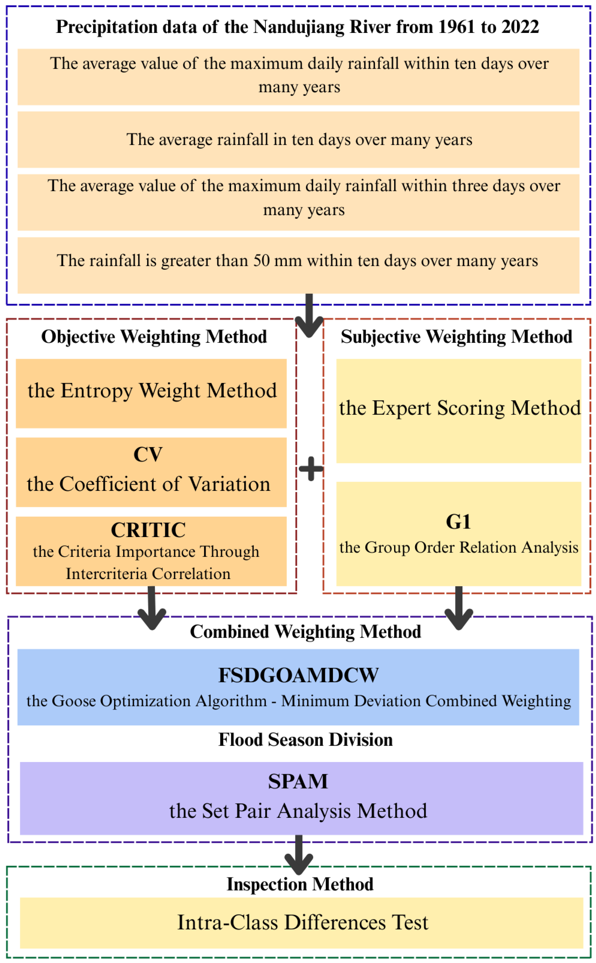
2. Methodology

2.1. Objective and Subjective Weighting Methods for Determining Indicator Weights

The drawing software used in this paper is Origin 2024 and ArcGIS10.8, the programming software is Matlab R2022b, the formula editing software is MathType 6.0 Equation, the software used for data organization is Microsoft Office Excel 2019, and the word processing software used is Microsoft Office Word 2019.

This chapter introduces a methodological framework integrating an objective weighting method (Entropy Weight, CV, CRITIC), a subjective weighting method (Expert Scoring, G1 method), and hybrid optimization. Based on the weights obtained by the subjective and objective weighting method, a Minimum Deviation model is established with the combined weight coefficients as the decision variable. The GOA is used to solve the optimization model to obtain the final combined weight. Combining the obtained combined weight, SPAM is adopted for flood season division. The final division results are evaluated based on the Intra-Class Differences analysis (Figure 1).

In the study of flood season division, four precipitation indicators are selected to characterize precipitation features from multiple dimensions for accurately reflecting the hydrological laws of the flood season. The multi-year average of the maximum daily rainfall within ten days focuses on short-term extreme precipitation intensity, while the multi-year average of ten-day rainfall reflects cumulative precipitation. The multi-year average of the maximum daily rainfall within three consecutive days emphasizes precipitation intensity and superposition effects; the multi-year frequency of rainfall exceeding 50 mm within ten days highlights the probability of extreme precipitation [28]. This indicator combination is scientific in three aspects: it achieves multi-dimensional coverage of precipitation intensity, cumulative amount, and extreme event frequency to comprehensively depict the “intensity-duration-frequency” characteristics of flood season precipitation; adapts to different ten-day and three-day time scales to cover both short-term extreme events and medium-to-long-term precipitation trends, in line with the precipitation pattern of the Nandujiang River Basin, influenced by typhoons and monsoons; and has data operability because it is calculated from historical daily precipitation data with mature statistical methods, facilitating integration with other hydrological models [29].

2.1.1. Calculation of Indicator Weights Using the Entropy Weight Method

As a representative objective weighting method, the Entropy Weight method determines weights by measuring data variability via information entropy. Higher entropy implies more uniform (less dispersed) data, weaker discriminability, and smaller weight; lower entropy indicates stronger discriminative power and higher weight [30]. This method involves the following steps:

Step 1 

Calculate the indicator weight matrix.

For sample i and indicator j, compute proportion P_ij using the following formula:

$${\mathrm{p}}_{\mathrm{i}\mathrm{j}}={\displaystyle \frac{{\mathrm{x}}_{\mathrm{i}\mathrm{j}}}{\sum _{\mathrm{i}=1}^{\mathrm{m}}{\mathrm{x}}_{\mathrm{i}\mathrm{j}}}},$$

(1)

In the formula, m is the number of samples, n is the number of indicators, and x_ij is the value of the j-th indicator for the i-th sample;

Step 2 

Compute the information entropy.

Calculate entropy E_j of j-th indicator using the following formula:

$${\mathrm{E}}_{\mathrm{j}}=-{\displaystyle \frac{1}{\mathrm{l}\mathrm{n}\left(\mathrm{m}\right)}}{\sum }_{\mathrm{i}=1}^{\mathrm{m}}{\mathrm{p}}_{\mathrm{i}\mathrm{j}}\mathrm{l}\mathrm{n}\left({\mathrm{p}}_{\mathrm{i}\mathrm{j}}\right),$$

(2)

Normalize E_j and compute the entropy redundancy D_j = 1 − E_j. A larger D_j indicates more effective information;

Step 3 

Compute the indicator weights.

Sum redundancy values D_k and then obtain weight w_j, as shown in the following formula:

$${\mathrm{w}}_{\mathrm{j}}={\displaystyle \frac{{\mathrm{D}}_{\mathrm{j}}}{\sum _{\mathrm{k}=1}^{\mathrm{n}}{\mathrm{D}}_{\mathrm{k}}}}$$

(3)

In the above formula, w_j is the weight of the j-th indicator, D_j is its entropy redundancy, and k refers to the indicator index.

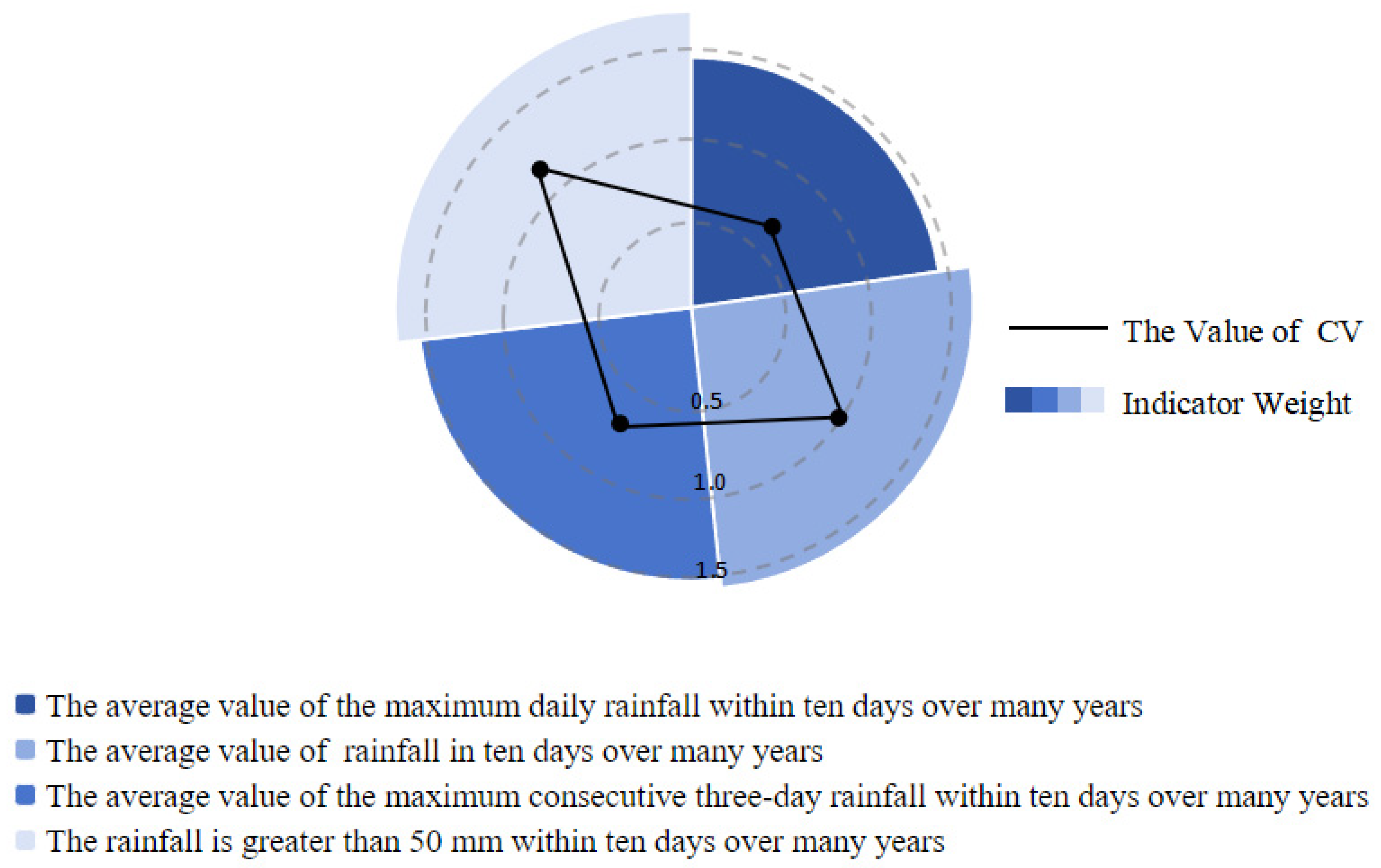
2.1.2. Calculation of Indicator Weights Using the Coefficient of Variation Method

The CV method is a technique that assigns weights in accordance with the information content of indicators using the following logic: a higher level of variability of an indicator leads to greater importance of that indicator, and consequently, results in a higher weight being assigned to it [31]. The specific implementation steps are as follows:

Step 1  

Calculate the mean.

For m samples (each with n indicators x_i1, x_i2, …, x_in), first calculate the mean value of each indicator using the following formula:

$${\overline{\mathrm{x}}}_{\mathrm{j}}={\displaystyle \frac{1}{\mathrm{m}}}{\sum }_{\mathrm{i}=1}^{\mathrm{m}}{\mathrm{x}}_{\mathrm{i}\mathrm{j}},\mathrm{j}=\mathrm{1,2},3,\dots ,\mathrm{n};$$

(4)

Step 2  

Calculate the standard deviation.

The standard deviation s_j of the j-th indicator is computed as follows:

$${\mathrm{s}}_{\mathrm{j}}=\sqrt{{\displaystyle \frac{1}{\mathrm{m}-1}}{\sum }_{\mathrm{i}=1}^{\mathrm{m}}{\left({\mathrm{x}}_{\mathrm{i}\mathrm{j}}-\overline{{\mathrm{x}}_{\mathrm{j}}}\right)}^2};$$

(5)

Step 3  

Calculate the CV.

The CV v_j for the j-th indicator is calculated as follows:

$${\mathrm{v}}_{\mathrm{j}}={\displaystyle \frac{{\mathrm{s}}_{\mathrm{j}}}{{\overline{\mathrm{x}}}_{\mathrm{j}}}};$$

(6)

Step 4  

Calculate the weights.

The weight of each indicator is calculated using the following formula:

$${\mathrm{w}}_{\mathrm{j}}={\displaystyle \frac{{\mathrm{v}}_{\mathrm{j}}}{{\sum }_{\mathrm{k}=1}^{\mathrm{n}}{\mathrm{v}}_{\mathrm{k}}}}.$$

(7)

2.1.3. Calculation of Indicator Weights Using the CRITIC (Criteria Importance Through Intercriteria Correlation) Method

The CRITIC method is an objective weighting technique. It quantifies indicator contrast intensity (via standard deviation) and inter-indicator conflict (via correlation coefficients) to construct an information matrix. More information-rich indicators get higher weights [32]. The specific steps are as follows:

Step 1  

Calculate correlations between indicators.

The inconsistency between the j-th indicator and other indicators is evaluated using a correlation coefficient matrix R = (r_jk)_m×n, calculated as follows:

$${\mathrm{r}}_{\mathrm{j}\mathrm{k}}={\displaystyle \frac{\sum _{\mathrm{i}=1}^{\mathrm{m}}\left({\mathrm{x}}_{\mathrm{i}\mathrm{j}}-{\stackrel{-}{\mathrm{x}}}_{\mathrm{j}}\right)\left({\mathrm{x}}_{\mathrm{i}\mathrm{k}}-{\stackrel{-}{\mathrm{x}}}_{\mathrm{k}}\right)}{\sqrt{\sum _{\mathrm{i}=1}^{\mathrm{m}}{\left({\mathrm{x}}_{\mathrm{i}\mathrm{j}}-{\stackrel{-}{\mathrm{x}}}_{\mathrm{j}}\right)}^2\sum _{\mathrm{i}=1}^{\mathrm{m}}{\left({\mathrm{x}}_{\mathrm{i}\mathrm{k}}-{\stackrel{-}{\mathrm{x}}}_{\mathrm{k}}\right)}^2}}},$$

(8)

In the formula, r_jk denotes the Pearson correlation coefficient between the j-th and k-th indicators.

The conflict intensity of the j-th indicator f_j is given by the following formula:

$${\mathrm{f}}_{\mathrm{j}}={\sum }_{\mathrm{k}=1,\mathrm{k}\ne \mathrm{j}}^{\mathrm{n}}\left(1-{\mathrm{r}}_{\mathrm{j}\mathrm{k}}\right),$$

(9)

A higher f_j is more unique information;

Step 2  

Calculate the amount of information.

The information content of the j-th indicator c_j is calculated as follows:

$${\mathrm{c}}_{\mathrm{j}}={\mathrm{s}}_{\mathrm{j}}\times {\mathrm{f}}_{\mathrm{j}},$$

(10)

In the formula, c_j represents the information of the j-th indicator, integrating its dispersion (standard deviation) and conflict (correlation). Greater dispersion and stronger conflict mean higher information value;

Step 3  

Calculate indicator weights.

The weight w_j of each indicator is computed using the following formula:

$${\mathrm{w}}_{\mathrm{j}}={\displaystyle \frac{{\mathrm{c}}_{\mathrm{j}}}{\sum _{\mathrm{k}=1}^{\mathrm{n}}{\mathrm{c}}_{\mathrm{k}}}}.$$

(11)

2.2. Subjective Weighting Methods for Determining Indicator Weights

2.2.1. Determining Indicator Weights Using the Expert Scoring Method

The Expert Scoring Method, a subjective weighting technique via the Delphi process, uses experts’ experience to assess indicator relationships and set weights [33]. The Expert Scoring in this study will consist of five senior experts in the field of hydrology and water resources, and the scoring for corresponding indicators will be carried out using a 100-point scale as the standard. The specific scoring procedures and fundamental steps are as follows:

Step 1  

Expert Selection: Pick experts with flood season division experience; explain weight definitions, rules, and recording;

Step 2  

List Compilation: List all indicators with weight ranges, quantified via the scoring scale;

Step 3  

Scoring: Distribute the list to experts for repeated evaluation (steps 4–9) until scores stabilize;

Step 4  

Individual Scoring: Experts score indicators by perceived importance;

Step 5  

Discussion and Revision: Experts discuss scores; revisit inconsistencies, rescore to reach consensus;

Step 6  

Total Score Calculation: Sum scores per expert across indicators;

Step 7  

Individual Weight Calculation: Compute indicator weight as (its score/expert’s total score);

Step 8  

Group Average Weight Calculation: Average weights across experts to obtain “group average weight”;

Step 9  

Comparative Display: Compare averages with step 7 individual weights to check discrepancies/rationality;

Step 10  

Finalization: Repeat scoring loop (steps 4–9) if discrepancies exist. Finalize group average weights once w_j agreed for decision–making.

2.2.2. Determining Indicator Weights Using the G1 Method (Group Order Relation Analysis)

The G1 method, a subjective weighting technique based on expert judgment, ranks indicators by importance and quantifies differences. More intuitive and efficient than AHP [34] (no complex pair-wise comparisons/consistency checks), it uses h_j (relative importance ratio of adjacent indicators). The method proceeds as follows:

Step 1  

Establish the Order Relation.

Experts rank n indicators x₁, x₂, …, x_n as x₁ > x₂> … > x_n, where “>” indicates greater importance;

Step 2  

Assess Relative Importance Between Adjacent Indicators.

Experts assign h_j for adjacent indicators x_j−1 and x_j, satisfying the following equation:

$${\mathrm{h}}_{\mathrm{j}}={\displaystyle \frac{{\mathrm{w}}_{\mathrm{j}-1}}{{\mathrm{w}}_{\mathrm{j}}}},\mathrm{j}=\mathrm{2,3},\dots ,\mathrm{n},$$

(12)

In the formula, w_j is the weight of indicator x_j. A higher h_j indicates a large importance gap;

Step 3  

Calculate Weight Coefficients.

Weights are computed sequentially using the following formula:

$${\mathrm{w}}_{\mathrm{j}}={\left(1+{\sum }_{\mathrm{j}=2}^{\mathrm{n}}{\prod }_{\mathrm{j}=\mathrm{k}}^{\mathrm{n}}{\mathrm{h}}_{\mathrm{j}}\right)}^{-1},$$

(13)

$${\mathrm{w}}_{\mathrm{j}-1}={\mathrm{h}}_{\mathrm{j}}{\mathrm{w}}_{\mathrm{j}},\mathrm{j}=\mathrm{n},\mathrm{n}-1,\dots ,2.$$

(14)

2.3. Optimal Combination Weights via the Goose Optimization Algorithm (GOA)

To mitigate the heterogeneity and bias between subjective and objective weighting methods, this study establishes a combined weighting framework. A multi-objective optimization model based on the Minimum Deviation method is constructed to derive combination weights. This approach seeks an optimal weighting solution by balancing subjective and objective information [35].

First, it is crucial to clarify how subjective and objective weights are integrated. Subjective weights, reflecting expert experience and qualitative judgments, and objective weights, derived from data-driven statistical analyses, are combined through a linear superposition manner. Specifically, we assign preference coefficients α_i (i = 1, 2, …, q) to each set of subjective or objective weights. These coefficients act as “bridges” to fuse different weight results, with the goal of minimizing the overall deviation between the combined weights and each original single weight, thus achieving a more comprehensive and reasonable weighting outcome.

The GOA, an emerging swarm intelligence technique, simulates the cooperative behavior of geese during migration. With its efficient search mechanism and strong global convergence capabilities, GOA demonstrates outstanding performance in solving various optimization problems. In this study, the GOA is applied to solve the combination weighting problem based on the principle of minimum deviation, aiming to more accurately and fairly assess the importance of indicators, thereby aligning final decisions more closely with real-world scenarios.

This method primarily involves collecting multiple subjective and objective weight results, defining a deviation function with the objective of minimizing the deviation between the combined weights and each single weight, and solving the optimal combination coefficients using the GOA. The GOA is employed to solve the weight optimization model established using the Minimum Deviation method [24], with the objective of achieving a quantitatively integrated weighting scheme. Let u denote the index of a goose individual, q the number of weighting methods, and t the number of iterations. The detailed steps are as follows:

Step 1  

Initialize the Goose Population.

Define the population size N. Each goose individual represents a potential set of preference coefficients α = (α₁, α₂, …, α_q). Randomly initialize each goose’s position vector y_u(0), ensuring 0 ≤ α ≤ 1 and ${\sum }_{i=1}^q$α_i = 1. This can be done by generating q random values in [0, 1] and normalizing them. Initialize the velocity vector v_u(0) randomly for each goose, typically with small magnitudes to prevent overly large initial search steps;

Step 2  

Define the Fitness Function.

The fitness function is defined based on the objective function of the Minimum Deviation Combination Weighting method, as follows:

$$\mathrm{F}\left(\mathsf{\alpha }\right)={\sum }_{\mathrm{j}=1}^{\mathrm{n}}{\sum }_{\mathrm{k}=1}^{\mathrm{q}}{\sum }_{\mathrm{l}=1}^{\mathrm{q}}\left|{\sum }_{\mathrm{i}=1}^{\mathrm{q}}{\mathsf{\alpha }}_{\mathrm{i}}{\mathsf{\mu }}_{\mathrm{i}\mathrm{j}}-{\sum }_{\mathrm{i}=1}^{\mathrm{q}}{\mathsf{\alpha }}_{\mathrm{i}}{\mathsf{\mu }}_{\mathrm{k}\mathrm{j}}\right|,$$

(15)

In the formula, μ_kj and μ_ij denote the weight of indicator j determined by the k-th and -th method, respectively. A smaller fitness value indicates a more optimal preference coefficient combination;

Step 3  

Update Goose Positions.

Dynamically update step sizes: For the leader goose, use α(t) = α₀(1 − t/T_max)²; for followers, use β(t) = β₀(1 − t/T_max)². Update the leader’s position by selecting the goose with the minimum fitness value and make direction adjustment with the probability of p.

The position update formula is:

$${\mathrm{y}}_{\mathrm{l}\mathrm{e}\mathrm{a}\mathrm{d}\mathrm{e}\mathrm{r}}\left(\mathrm{t}+1\right)={\mathrm{y}}_{\mathrm{l}\mathrm{e}\mathrm{a}\mathrm{d}\mathrm{e}\mathrm{r}}\left(\mathrm{t}\right)+\mathsf{\alpha }\left(\mathrm{t}\right)\left(\mathrm{r}-{\displaystyle \frac{1}{2}}\right)\odot {\mathrm{y}}_{\mathrm{l}\mathrm{e}\mathrm{a}\mathrm{d}\mathrm{e}\mathrm{r}}\left(\mathrm{t}\right),$$

(16)

Update the followers’ positions by moving them toward the leader using:

$${\mathrm{y}}_{\mathrm{u}}\left(\mathrm{t}+1\right)={\mathrm{y}}_{\mathrm{u}}\left(\mathrm{t}\right)+\mathsf{\beta }\left(\mathrm{t}\right)\left(\mathrm{y}\mathrm{l}\mathrm{e}\mathrm{a}\mathrm{d}\mathrm{e}\mathrm{r}\left(\mathrm{t}\right)-\mathrm{y}\mathrm{u}\left(\mathrm{t}\right)\right),\mathrm{u}\ne \mathrm{l}\mathrm{e}\mathrm{a}\mathrm{d}\mathrm{e}\mathrm{r},$$

(17)

After position update, the new coordinates must satisfy 0 ≤ α ≤ 1 and ${\sum }_{i=1}^q$α_i = 1. If not, corrections and normalization are required;

Step 4  

Update Individual and Global Bests.

Update personal best: If the current fitness F(y_u(t + 1)) is better than the historical best, update the individual’s best position.

Global best: Among all individuals’ bests, the one with the lowest fitness is compared to the current global best. If it is better than the current global optimal solution, then update the global optimal position;

Step 5  

Termination Criteria.

Set a maximum iteration count T_max or a minimum fitness threshold ϵ. When either condition is met, the iteration halts and the current best preference coefficient α is deemed optimal. The final combination weights W_j for each indicator are calculated using the following formula:

$${\mathrm{W}}_{\mathrm{j}}={\sum }_{\mathrm{l}=1}^{\mathrm{q}}{\mathsf{\alpha }}_{\mathrm{l}}{\mathsf{\mu }}_{\mathrm{l}\mathrm{j}},$$

(18)

To summarize, the GOA achieves combined weighting by simulating the cooperative behavior of migratory geese: A population of “geese” is initialized, where each goose represents a set of preference coefficients used to weight subjective and objective individual weights. The fitness function is defined as the total deviation between the combined weights and all individual weights, ensuring the combined weights fit all individual weights of each indicator. The leader goose (with the smallest fitness) explores new directions through random perturbations, while follower geese move toward the leader with step sizes that decay over iterations, balancing global exploration and local optimization. After tracking the optimal coefficients through iterations, the combined weights are calculated by weighting all individual weights with the optimal coefficients, integrating subjective and objective information for flood season division.

2.4. Validation of Division Methods Under Different Weighting Schemes Using Intra-Class Differences

The Intra-Class Differences method evaluates division effectiveness by assessing data dispersion Intra Classes, assuming that good division has low Intra-Class Differences [36]. The procedure is as follows:

Step 1  

Compute Class Mean.

For class ω_d with n samples x_d1, x_d2, …, x_d, the class mean is given as follows:

$${\overline{\mathrm{x}}}_{\mathrm{d}}={\displaystyle \frac{1}{\mathrm{n}}}{\sum }_{\mathrm{j}=1}^{\mathrm{n}} {\mathrm{x}}_{\mathrm{d}\mathrm{j}},$$

(19)

Step 2  

Compute Intra-Class Differences.

The Intra-Class Differences of class $S_d^2$ is as follows:

$${\mathrm{S}}_{\mathrm{d}}^2={\displaystyle \frac{1}{\mathrm{n}}}{\sum }_{\mathrm{j}=1}^{\mathrm{n}} ({\mathrm{x}}_{\mathrm{d}\mathrm{j}}-{\overline{\mathrm{x}}}_{\mathrm{d}}{)}^2.$$

(20)

Step 3  

Compute Overall Intra-Class Differences.

Aggregate class differences weighted by sample proportions to obtain the overall Intra-Class Differences $S_W^2$. Let N be the total number of samples:

$$\mathrm{N}={\sum }_{\mathrm{d}=1}^{\mathrm{C}} \mathrm{n},$$

(21)

$${\mathrm{S}}_{\mathrm{w}}^2={\sum }_{\mathrm{d}=1}^{\mathrm{C}} {\displaystyle \frac{\mathrm{n}}{\mathrm{N}}}{\mathrm{S}}_{\mathrm{d}}^2.$$

(22)

In the formula, $S_W^2$ represents the overall Intra-Class Differences.

2.5. Set Pair Analysis for the Division of Flood and Non-Flood Periods

The Set Pair Analysis method (SPAM) is based on the theory of opposition and unity in system science. It compares the similarity, difference, and opposition of a particular feature. When dividing the flood season, two categories are first defined: flood season and non-flood season [19]. For any given time period (which can also be considered as an independent set), the degree of association with these two categories is evaluated. Afterward, based on the obtained association degree, time periods that have a stronger association with the flood season set are classified as flood seasons [37]. The steps are as follows:

Step 1  

Determine the threshold for indicators.

For the sample matrix, each sample at a time point consists of a series of indicators, which can be represented as Z_i = {x_i1, x_i2, …, x_im}, as shown in the formula below:

$${\mathsf{\beta }}_{\mathrm{j}}={\displaystyle \frac{\left({\sum }_{\mathrm{i}=1}^{\mathrm{m}}{\mathrm{x}}_{\mathrm{i}\mathrm{j}}\right)}{\mathrm{m}}}.$$

(23)

In this formula, β_j represents the threshold for the j-th indicator.

The threshold between flood and non-flood season for each indicator are then determined. When x_ij > β_j, it belongs to the flood season; when x_ij ≤ β_j, it belongs to the non-flood season.

Step 2  

Data Symbolization.

Based on the above threshold, when x_ij > β_j, denote it as √; when x_ij ≤ β_j, denote it as ×. Using this rule, the flood period state set can be defined as B₁ = {√, √, …, √} and the non-flood period state set can be defined as B₂ = {×, ×, …, ×}.

When classifying flood periods, each time period can only exhibit a state that is either consistent with, or different than, the flood or non-flood period. Therefore, only binary associations are considered. In the sample matrix, each observation at a time point consists of a series of indicators, forming a complete set, represented as Z_i = {x_i1, x_i2, …, x_im}.

The aforementioned method can be used to determine the threshold β_j between flood and non-flood periods for each indicator. Next, for the samples of each time period, we calculate the weighted binary correlation between them and the flood and non-flood seasons. The specific formula is as follows:

$${\mathrm{V}}_{\mathrm{i}1}={\mathrm{W}}_{\mathrm{i}1}+{\mathrm{W}}_{\mathrm{i}2}+\cdots +{\mathrm{W}}_{\mathrm{i}\mathrm{S}},$$

(24)

$${\mathrm{V}}_{\mathrm{i}2}={\mathrm{W}}_{\mathrm{i}1}+{\mathrm{W}}_{\mathrm{i}2}+\cdots +{\mathrm{W}}_{\mathrm{i}\mathrm{F}}$$

(25)

In this formula, the weighted binary correlation is defined. Here, V_i1 is used to measure the degree of association between a specific period and the flood season set, while {W_i1, W_i2, …, W_is} represents the weight values of all the indicators marked with √ within the set Z_i. S denotes the number of indicators marked with √, which can be interpreted as the number of matching features between the set Z_i and the flood season set. Similarly, V_i2 is used to evaluate the correlation between the same time period and the non-flood season set; {W_i1, W_i2, …, W_iF} corresponds to the weights of all the indicators marked with × within the set Z_i; and F refers to the number of these marked indicators (that is, the total number of the same characteristics between the set Z_i and the non-flood season set).

For any time period i, its flood season attribute can be determined according to the following rule: If V_i1 > V_i2, then i is the flood season. Otherwise, i is the non-flood season.

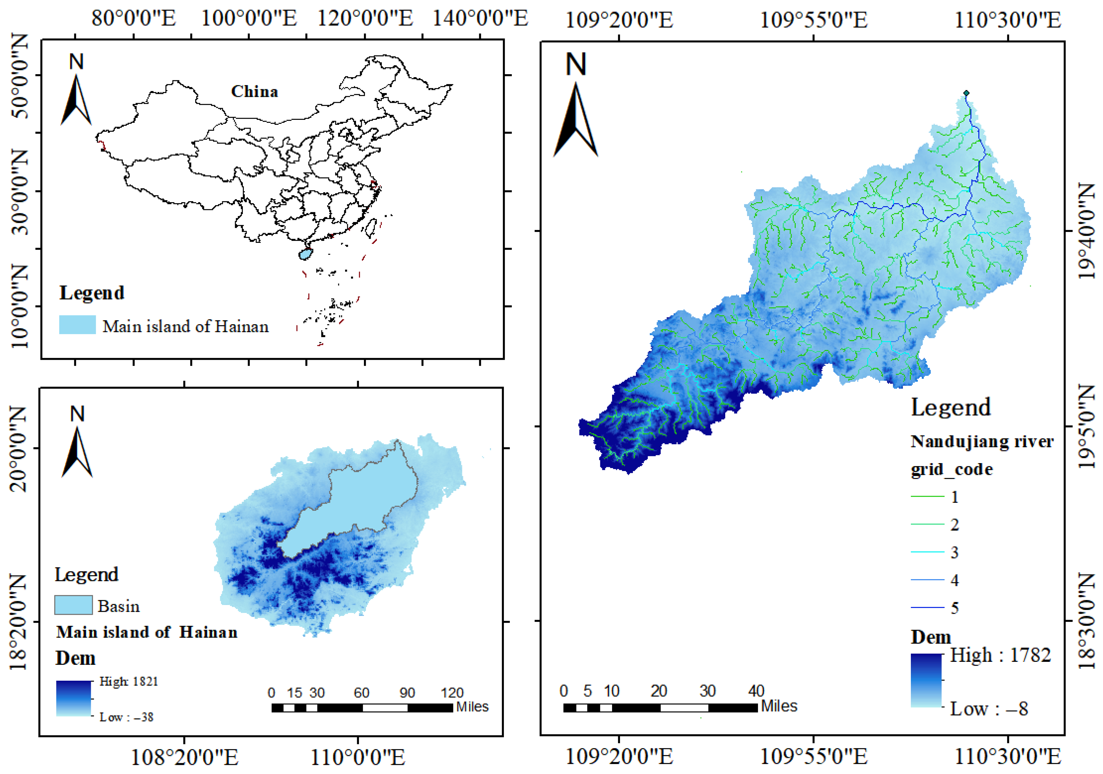
3. Case Study

The Nandujiang River basin is located in northern Hainan Province, China. Its watershed area is 445.12 square kilometers and the land use types within the basin are mainly cultivated land and rubber plantations, etc. The basin has a multi-year average rainfall depth of 1935 mm, decreasing from upstream to downstream. Meanwhile, the multi-year average temperature within the basin is 23.5 °C [38]. The river drops 703 m along its course, with an average channel gradient of 0.716% [39]. This study uses daily precipitation records from 1961 to 2022 (62 years) as the main dataset, with the geographical distribution of the basin shown in Figure 2.

4. Data Preprocessing and Results

4.1. Data Preprocessing for Flood Season Division

Daily precipitation measurements for all twelve months were used to compute and classify flood season data. Based on the raw records, four core evaluation indicators were selected: the average value of the maximum daily rainfall within ten days over many years; the average value of rainfall in ten days over many years; the average value of the maximum consecutive three-day rainfall within ten days over many years; and the rainfall is greater than 50 mm within ten days over many years. An ordered sample set X was constructed, comprising 36 samples, each represented by a four-dimensional feature vector.

4.2. Combination Weight Calculation and Indicator Symbolization

Indicator weights were computed as described in Section 1 (see Figure 3). Following the procedure in Section 2, each indicator value was symbolized; values exceeding the threshold were denoted as “√” and values at or below the threshold as “×”. The symbolization results are listed in

Table 1. Symbolic indicators of flood season division in the Nandujiang River.

Month	Ten Days	Indicator One	Indicator Two	Indicator Three	Indicator Four
1	1	×	×	×	×
	2	×	×	×	×
	3	×	×	×	×
2	1	×	×	×	×
	2	×	×	×	×
	3	×	×	×	×
3	1	×	×	×	×
	2	×	×	×	×
	3	×	×	×	×
4	1	×	×	×	×
	2	×	×	×	×
	3	×	×	×	×
5	1	√	√	√	×
	2	√	√	√	×
	3	√	√	√	×
6	1	√	√	√	×
	2	√	√	√	×
	3	√	√	√	×
7	1	√	√	√	×
	2	√	√	√	√
	3	√	√	√	√
8	1	√	√	√	√
	2	√	√	√	√
	3	√	√	√	√
9	1	√	√	√	√
	2	√	√	√	√
	3	√	√	√	√
10	1	√	√	√	√
	2	√	√	√	√
	3	√	√	√	√
11	1	√	×	×	√
	2	×	×	×	×
	3	×	×	×	×
12	1	×	×	×	×
	2	×	×	×	×
	3	×	×	×	×

Note: The first indicator is the average value of the maximum daily rainfall within ten days over many years; the second indicator is the average rainfall within ten days over many years; the third indicator is the average value of the maximum daily rainfall within three days over many years; the fourth indicator is the rainfall is greater than 50 mm within ten days over many years. Explanations of the symbols can be found in Section 4.2, at the top of Table 1.

.

These four indicators quantify precipitation from complementary perspectives, offering a comprehensive characterization of temporal rainfall patterns. After symbolization for the Nandujiang River basin, under the “The average value of the maximum daily rainfall within ten days over many years” indicator, the flood period spans 1 May to 10 November; under “The average rainfall in ten days over many years”, the flood period spans from 1 May to 30 October; under “The average value of the maximum daily rainfall within three days over many years.”, the flood period spans from 1 May to 30 October; and under “The rainfall is greater than 50 mm within ten days over many years”, the flood period spans from 11 July to 10 November. The longest flood period corresponds to the first indicator, while the shortest corresponds to the last, indicating that the first period’s extreme values are more dispersed and the last period’s are more concentrated. At the same time, the latter exhibits a higher variance, consistent with results from the CV and Entropy Weight methods, providing further evidence of the GOA’s superior solution quality and efficiency. The combined weights of various indicators for the division of flood seasons are shown in Figure 3.

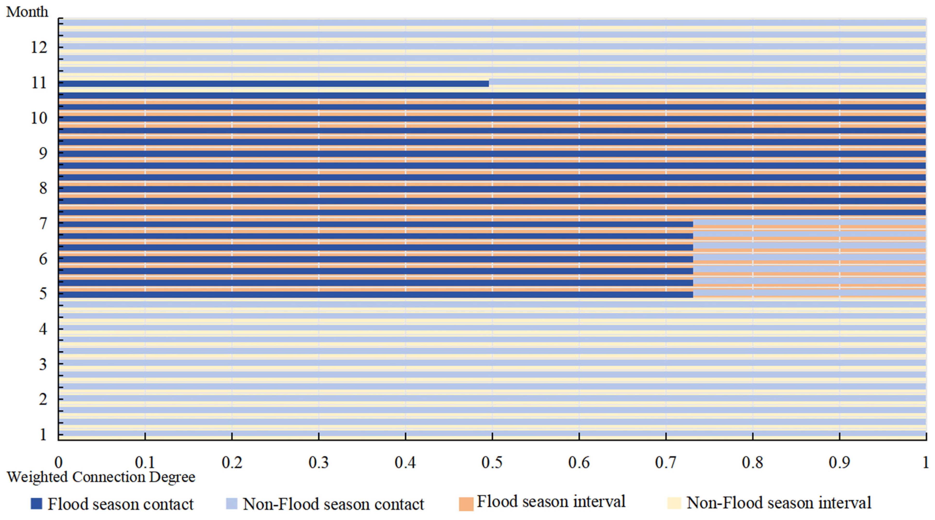
4.3. Flood Season Division Using Set Pair Analysis

Following the symbolization process, and based on the results in Table 1 and the methodology outlined in Section 2, the degree of connection between each ten-day period and both the flood and non-flood seasons was calculated using Equations (24) and (25). The results are shown in Figure 4 and Figure 5.

Using the criteria defined in Section 2, each time period was classified as either a flood or non-flood season. The resulting delineation identifies the flood season as spanning from 1 May to 30 October. This aligns closely with the findings of this study. Moreover, the delineated period encompasses the core of Hainan’s rainy season and accounts for the overlapping effects of typhoons and strong convective weather, making the division highly relevant to the practical needs of regional flood control planning. Combined with the flood frequency data in Figure 5, the characteristics of the annual flood occurrences in Hainan can be summarized as follows. The main floods in Hainan throughout the year are concentrated from May to October and the flood frequency during this period accounts for 88% of the whole year. Among these, due to the frequent occurrence of typhoons and strong rainfall, August and September become the relatively peak periods of flood frequency. The occurrence periods of most flood events are highly consistent with the flood season delineation results, which also verifies the rationality of the flood season delineation from the perspective of practical data, providing an intuitive and powerful support for regional flood control planning.

5. Discussion

5.1. Comparative Analysis of the Combined Weighting Method and the Single Weighting Method

To evaluate the performance of the proposed model, the flood season division results obtained using the combined weighting method were compared with those derived from single subjective and objective weighting approaches. The results were compared using the Intra-Class Differences method, as outlined in Section 1. The specific design is as follows. All combinations are based on the SPAM main framework for flood season division. The difference lies in the combination of SPAM with different weights, which are derived from combinatorial weights and weights obtained through subjective–objective weighting methods. Finally, different flood season division results are obtained by combining SPAM with different weights and the Intra-Class Differences is used to evaluate these different division results. The weighting scheme corresponding to the flood season division plan with the best evaluation result is defined as the optimal weighting method, thus realizing the comparison of different weighting methods. The results are shown in Figure 6.

As can be seen from Figure 6, the average total number of days in the flood season calculated by various methods is 189.6 days, which is basically consistent with that of a study by Li et al. [20]. The shortest time domain of the flood season is from 1 May to 30 October (combined weight method); the longest time domain of the flood season is from 1 May to 10 November (G1 method and CV method). From the perspective of Intra-Class Differences values, the minimum value is 10.01 (combined weight method), the maximum value is 10.24 (G1 method and CV method), and the average value is 10.15. Increasing the number of weighting methods can lead to the cancellation of random errors during the combination process [14]. Among all the methods, the combination weighting approach yielded the smallest Intra-Class Differences, indicating that the flood season division achieved through SPAM with combined weights is closest to the ideal scenario. A smaller Intra-Class Differences signifies that hydrometeorological characteristics within the classified periods are more consistent, thus supporting a more reasonable division. In addition, although the Entropy Weight method is widely used, it is highly sensitive to data errors and ignores the correlations between indicators. This may lead to deviations in the division of the flood season. Meanwhile, it neglects the physical meanings among indicators. In cases with modifying indicators or under other circumstances, the Entropy Weight method may also result in significant fluctuations and poor stability [40]. The CV method assumes equal importance across indicators and only reflects discriminative power rather than actual importance, potentially resulting in unreasonable segmentation [41]. The CRITIC method may disregard the physical significance of indicators, thus undermining the rationality of the segmentation. Shorter flood season divisions offer several practical advantages: they allow for longer periods of time for water resource utilization; enable focused resource allocation to improve water utilization efficiency; streamline decision-making and implementation processes; and enhance emergency response capabilities. Moreover, by precisely capturing hydrometeorological characteristics, shorter flood season divisions reduce uncertainty in resource planning and risk management [42].

To further assess the rationality of different methods, a comparison was conducted between the Expert Scoring method and the combined weighting approach using data from the first ten days of November. The comparison results are presented in

Table 2. Membership degree of the flood season in the Nandujiang River flood season division (first decade of November) via Expert Scoring and Combined Weighting methods.

Method	Flood Season/Membership	Non-Flood Season/Membership
Expert Scoring method	0.500	0.500
Combined Weighting method	0.495	0.505

.

It can be seen that when the number of indicators is even, SPAM may yield an equal number of matching and mismatching symbols, leading to identical weighted affiliation degrees for flood and non-flood seasons under the Expert Scoring method—thus making it impossible to determine the season type. In contrast, the combined weighting method successfully distinguishes whether the period belongs to the flood or non-flood season. This demonstrates that the combined weighting approach can overcome ambiguities in special cases and ensures a more definitive division outcome.

It can be seen from the above table that the model in this paper has certain applicability for the division of flood seasons in river basins in tropical island regions and can provide support for water resource planning and management in tropical island regions.

5.2. Comparison of Optimization Algorithm Performance

In the realm of algorithm optimization research, comparing the performance of different intelligent algorithms is crucial for selecting suitable tools to tackle complex computational problems. This section focuses on analyzing and contrasting the Goose Optimization Algorithm (GOA) and the Genetic Algorithm (GA) [23], delving into their convergence characteristics and fitness value variations. Through the study of their behavior in a standard test function context, we aim to reveal the differences of these two algorithms, providing insights for their application in practical scenarios such as flood season division models.

Figure 7 shows that the GOA stabilizes by iteration T = 5, whereas the Genetic Algorithm stabilizes by T = 20; GOA achieves full convergence at T = 24, and Genetic Algorithm at T = 31. This comparison demonstrates that GOA converges more rapidly to the global optimum, enhancing search efficiency and accuracy while mitigating the risk of local optima [24]. In the test function, the Genetic Algorithm (GA) exhibits fluctuations multiple times. The reason lies in that the GA simulates the mechanisms of natural selection and genetics. During the mutation process, the generated individuals may deviate far from the current region of the optimal solution, thus causing the fitness values to fluctuate up and down. The GOA simulates the migration and foraging behaviors of a flock of geese. The search mechanism of GOA is relatively more stable and regular. The movement and behavior decisions of individuals are based on the overall state of the group and pre-set rules. Therefore, during the iteration process, the change in fitness values is more stable, and large–scale fluctuations are less likely to occur.

6. Conclusions

In view of the special hydrometeorological conditions of tropical islands and the singularity of weighting perspectives in the weighting process of flood season division indicators, the flood season division model proposed in this study, integrating the GOA with Minimum Deviation Combined weighting, has been validated through a case study in the Nandujiang River Basin, offering a robust flood season division framework for tropical island regions. By combining two subjective weighting methods (Expert Scoring, G1) and three objective methods (Entropy Weight, CV, CRITIC), the model addresses the limitations of single weighting approaches such as subjective bias or disregard for indicator physics. The specific process of calculating the combined weights is as follows. Based on the weights obtained by the subjective–objective weighting method, the Minimum Deviation method is adopted to establish an optimization model with combined weight coefficients as decision variables. Finally, the GOA is used to solve the optimization model to obtain the combined weights. The application of Set Pair Analysis (SPAM) using combined weights determined the flood season, demonstrating smaller Intra-Class Differences and higher discriminative power compared to single methods. This approach also overcomes classification ambiguities in special cases, providing a more reliable basis for flood control and water resource management. The main conclusions of this paper are as follows.

①

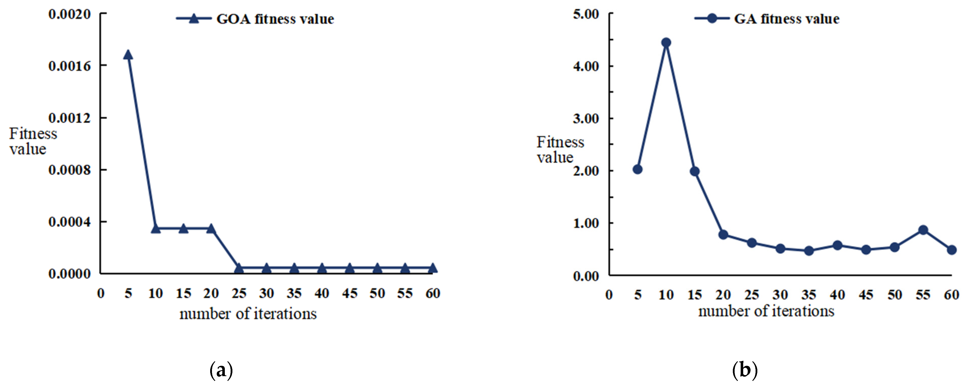
GOA converges faster than the Genetic Algorithm, stabilizing at T = 5 and achieving full convergence at T = 24;

②

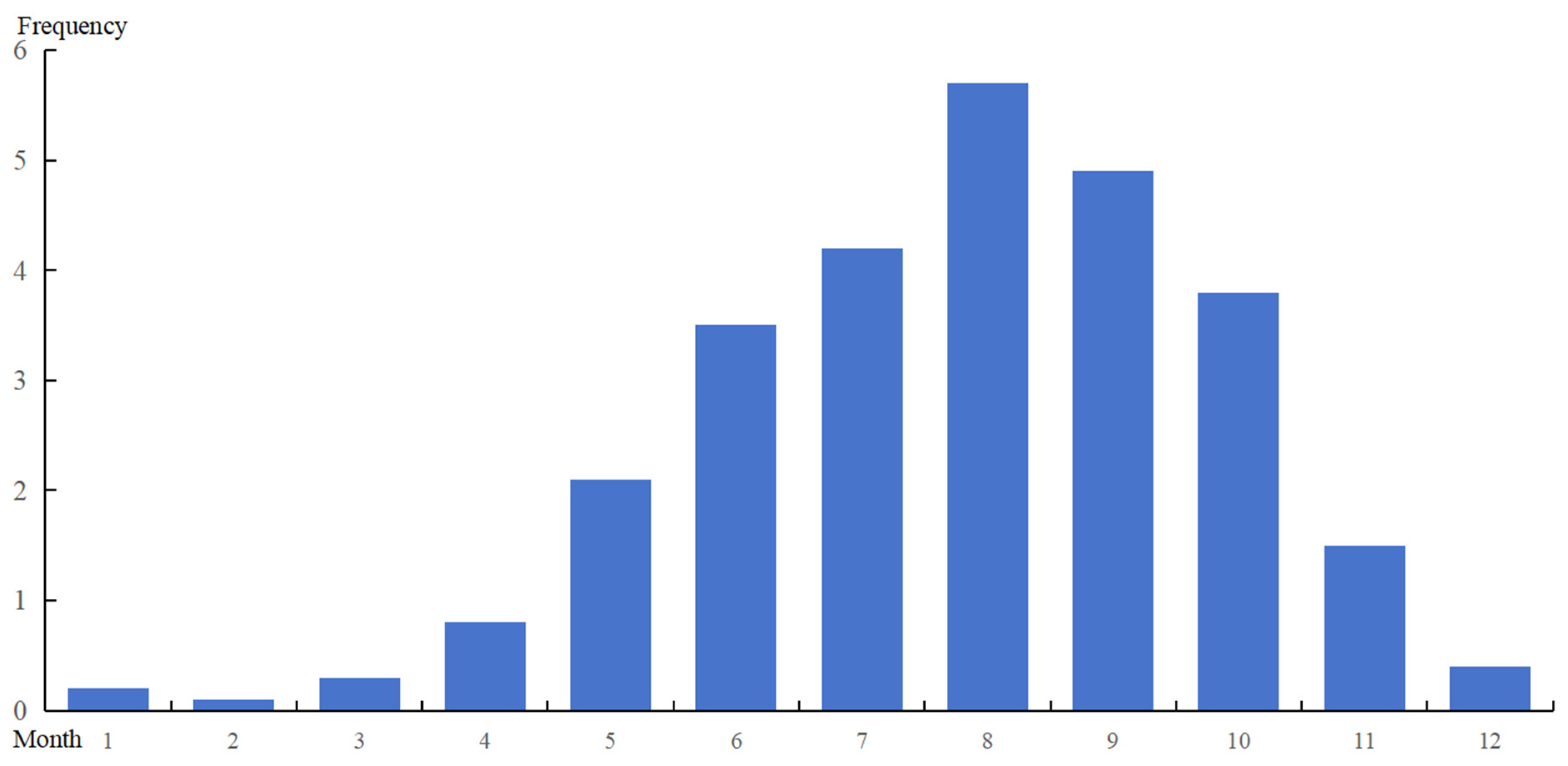
Based on the calculation results of the model in this paper, the flood season time domain of the Nandujiang River Basin is from 1 May to 30 October. This result can provide a certain reference basis for reservoir operation;

③

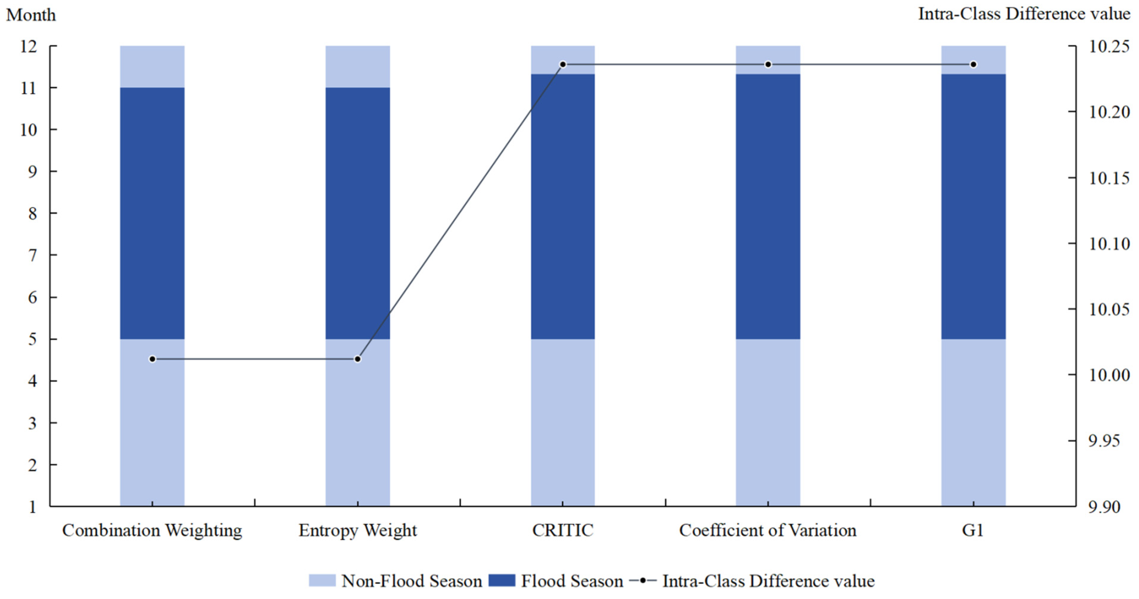
In the evaluation process based on Intra-Class Differences, the Intra-Class Differences of the model in this paper is the smallest, which is 10.01. The smallest Intra-Class Differences indicates that the division results based on the model in this paper have good Intra-Class similarity. Compared with the comparison models established based on subjective or objective weighting methods, the model in this paper has better consistency in flood season division in tropical island regions.

While this research highlights the model’s effectiveness, several directions for future investigation are evident. First, the model’s generalizability remains untested in other watersheds with distinct hydrological characteristics (e.g., monsoon-driven basins or regions with complex topographies). Validating the model across diverse ecosystems will refine its adaptability and identify potential limitations. Second, incorporating additional hydrological indicators (e.g., runoff dynamics, tidal influences) or climate change projections could enhance the model’s precision in dynamic environmental scenarios. Additionally, exploring hybrid optimization algorithms or integrating machine learning techniques may further improve convergence efficiency and weight assignment accuracy. This study presents a key approach to achieving sustainable water resource utilization. It scientifically divides the entire year into flood seasons (high-risk periods) and non-flood seasons (lower-risk periods), prioritizing flood control safety during high-risk phases while dynamically raising reservoir water levels to capture floodwater resources during lower-risk periods. This significantly enhances floodwater utilization, converting flood season abandoned water into valuable water sources in dry seasons. By ensuring safety, it effectively increases water supply, improves ecology, mitigates temporal and spatial water resource disparities, and supports long-term sustainable utilization.

References

- Li, Y.; Li, Y.; Feng, K.; Sun, K.; Cheng, Z. The Influence of Time Domain on Flood Season Segmentation by the Fisher Optimal Partition Method. Water 2024, 16, 580. [Google Scholar] [CrossRef]
- Fang, C.; Guo, S.; Duan, Y.; Duong, D. Two new approaches to dividing flood sub-seasons in flood season using the fractal theory. Chin. Sci. Bull. 2010, 55, 105–110. [Google Scholar] [CrossRef]
- Xu, Z.; Mo, L.; Zhou, J.; Zhang, X. Optimal dispatching rules of hydropower reservoir in flood season considering flood resources utilization: A case study of Three Gorges Reservoir in China. J. Clean. Prod. 2023, 388, 135975. [Google Scholar] [CrossRef]
- Jiang, H.; Wang, Z.; Ye, A.; Liu, K.; Wang, X.; Wang, L. Hydrological characteristic-based methodology for dividing flood seasons: An empirical analysis from china. Environ. Geol. 2019, 78, 399.1–399.9. [Google Scholar] [CrossRef]
- Ghosh, A.; Kar, S.K. Application of analytical hierarchy process (AHP) for flood risk assessment: A case study in Malda district of West Bengal, India. Nat. Hazards 2018, 94, 349–368. [Google Scholar] [CrossRef]
- Kwong, C.K.; Ip, W.H.; Chan, J.W.K. Combining scoring method and fuzzy expert systems approach to supplier assessment: A case study. Integr. Manuf. Syst. 2002, 13, 512–519. [Google Scholar] [CrossRef]
- Li, M.; Zhou, R.R.; Wang, Y.T.; Liu, D. Variable Fuzzy Sets Method for Flood Seasonality of Catchments. In Proceedings of the World Environmental and Water Resources Congress 2015, Austin, TX, USA, 17–21 May 2015; pp. 643–651. [Google Scholar]
- Chen, L.; Singh, V.P.; Guo, S.; Zhou, J.; Zhang, J.; Liu, P. An objective method for partitioning the entire flood season into multiple sub-seasons. J. Hydrol. 2015, 528, 621–630. [Google Scholar] [CrossRef]
- Malekinezhad, H.; Sepehri, M.; Pham, Q.B.; Hosseini, S.Z.; Meshram, S.G.; Vojtek, M.; Vojteková, J. Application of entropy weighting method for urban flood hazard mapping. Acta Geophys. 2021, 69, 841–854. [Google Scholar] [CrossRef]
- Thangjai, W.; Niwitpong, S.A.; Niwitpong, S. Confidence intervals for the common coefficient of variation of rainfall in Thailand. PeerJ 2020, 8, e10004. [Google Scholar] [CrossRef]
- Mu, Z.; Ai, X.; Ding, J.; Huang, K.; Chen, S.; Guo, J.; Dong, Z. Risk analysis of dynamic water level setting of reservoir in flood season based on multi-index. Water Resour. Manag. 2022, 36, 3067–3086. [Google Scholar] [CrossRef]
- Wang, S.; Yang, X. Flood season division based on correlation coefficient and optimum partition method of fisher. J. China Hydrol. 2011, 32, 1–5. [Google Scholar]
- Karunarathne, A.W.S.P.; Piyatilake, I.T.S. Determining Flood Risk Vulnerability Using Factor Analysis Approach. In 2021 6th International Conference on Information Technology Research (ICITR), Moratuwa, Sri Lanka, 1–3 December 2021; IEEE: Piscataway, NJ, USA, 2021; pp. 1–6. [Google Scholar]
- Mo, C.; Deng, J.; Lei, X.; Ruan, Y.; Lai, S.; Sun, G.; Xing, Z. Flood season staging and adjustment of limited water level for a multi-purpose reservoir. Water 2022, 14, 775. [Google Scholar] [CrossRef]
- Zhao, J.; Jin, J.; Zhu, J.; Xu, J.; Hang, Q.; Chen, Y.; Han, D. Water resources risk assessment model based on the subjective and objective combination weighting methods. Water Resour. Manag. 2016, 30, 3027–3042. [Google Scholar] [CrossRef]
- Ponhan, K.; Sureeyatanapas, P. A comparison between subjective and objective weighting approaches for multi-criteria decision making: A case of industrial location selection. Eng. Appl. Sci. Res. 2022, 49, 763–771. [Google Scholar]
- Ran, L.; Tan, X.; Xu, Y.; Zhang, K.; Chen, X.; Zhang, Y.; Li, M.; Zhang, Y. The application of subjective and objective method in the evaluation of healthy cities: A case study in Central China. Sustain. Cities Soc. 2021, 65, 102581. [Google Scholar] [CrossRef]
- Yao, H.; Dong, Z.; Jia, W.; Ni, X.; Chen, M.; Zhu, C.; Li, D. Competitive relationship between flood control and power generation with flood season division: A case study in downstream Jinsha River Cascade Reservoirs. Water 2019, 11, 2401. [Google Scholar] [CrossRef]
- Ma, P.; Han, L.; Liu, H.; Zhang, H. Fuzzy multi-objective optimization of EMT based on the minimum average weighted deviation algorithm. Energy Procedia 2017, 105, 2409–2414. [Google Scholar] [CrossRef]
- Li, J. A flood season division model considering uncertainty and new information priority. Water Resour. Manag. 2024, 38, 3755–3784. [Google Scholar] [CrossRef]
- Jhong, Y.D.; Chen, C.S.; Jhong, B.C.; Tsai, C.H.; Yang, S.Y. Optimization of LSTM parameters for flash flood forecasting using genetic algorithm. Water Resour. Manag. 2024, 38, 1141–1164. [Google Scholar] [CrossRef]
- Jiang, L.; Tajima, Y.; Wu, L. Application of Particle Swarm Optimization for Auto-Tuning of the Urban Flood Model. Water 2022, 14, 2819. [Google Scholar] [CrossRef]
- Zhai, L.; Feng, S. A novel evacuation path planning method based on improved genetic algorithm. J. Intell. Fuzzy Syst. 2022, 42, 1813–1823. [Google Scholar] [CrossRef]
- Pawan, Y.N.; Prakash, K.B.; Chowdhury, S.; Hu, Y.C. Particle swarm optimization performance improvement using deep learning techniques. Multimed. Tools Appl. 2022, 81, 27949–27968. [Google Scholar] [CrossRef]
- Hamad, R.K.; Rashid, T.A. GOOSE algorithm: A powerful optimization tool for real-world engineering challenges and beyond. Evol. Syst. 2024, 15, 1249–1274. [Google Scholar] [CrossRef]
- Zhang, J.; Xu, L.; Xia, L.; Yang, Q.; Chen, Z.; Dong, W. Comprehensive Evaluation Technology of Photovoltaic Power Station Power Generation Performance Based on Minimum Deviation Combined Weighting Method. In Proceedings of the 2022 IEEE 6th Conference on Energy Internet and Energy System Integration (EI2), Chengdu, China, 11–13 November 2022; IEEE: Piscataway, NJ, USA, 2022; pp. 880–885. [Google Scholar]
- Li, X.; Zhang, W.; Wang, X.; Wang, Z.; Pang, C. Evaluation on the risk of water inrush due to roof bed separation based on improved set pair analysis–variable fuzzy sets. Acs Omega 2022, 7, 9430–9442. [Google Scholar] [CrossRef]
- Jin, D.T.; Zhou, T.; Yang, X.H.; Lu, Y.; Wang, K.W. Assessment of regional water resource carrying capacity by the connection number of set pair analysis. Therm. Sci. 2024, 28, 2287–2294. [Google Scholar] [CrossRef]
- Wang, L.; Liu, Y.; Li, Z.; Yi, H.; Wang, Z.; Liu, H.; Wu, D.; Li, Y.; Liu, M. Distribution characteristics of terrestrial PGEs and its trend into the sea around Hainan Island, China. Sci. Total Environ. 2025, 963, 178372. [Google Scholar] [CrossRef]
- Zhu, Y.; Tian, D.; Yan, F. Effectiveness of entropy weight method in decision-making. Math. Probl. Eng. 2020, 2020, 3564835. [Google Scholar] [CrossRef]
- Sun, Y.; Liang, X.; Xiao, C. Assessing the influence of land use on groundwater pollution based on coefficient of variation weight method: A case study of Shuangliao City. Environ. Sci. Pollut. Res. 2019, 26, 34964–34976. [Google Scholar] [CrossRef]
- Žižović, M.; Miljković, B.; Marinković, D. Objective methods for determining criteria weight coefficients: A modification of the CRITIC method. Decis. Mak. Appl. Manag. Eng. 2020, 3, 149–161. [Google Scholar] [CrossRef]
- Gao, Z.; McCalley, J.; Meeker, W. A transformer health assessment ranking method: Use of model based scoring expert system. In Proceedings of the 41st North American Power Symposium, Starkville, MS, USA, 4–6 October 2009; IEEE: Piscataway, NJ, USA, 2009; pp. 1–6. [Google Scholar]
- Xie, X.J. Research on material selection with multi-attribute decision method and G1 method. Adv. Mater. Res. 2014, 952, 20–24. [Google Scholar] [CrossRef]
- Liu, D.H.; Yu, Q.; Ma, X.N.; Yin, D.; Zhang, W.G. Emergency response capability evaluation model based on minimum deviation combined weights. J. China Manag. Sci. 2014, 22, 79–86. [Google Scholar]
- Kotsia, I.; Pitas, I.; Zafeiriou, S. Novel multiclass classifiers based on the minimization of the within-class variance. IEEE Trans. Neural Netw. 2008, 20, 14–34. [Google Scholar] [CrossRef]
- Lu, X.D.; Qi, S.; Chen, J.D.; Guo, J.C.; Zhang, L.; Zhou, P. Spatiotemporal Distribution and Variation Trend of Rainfall Erosivity in the Nandu River Basin. J. Ecol. Rural. Environ. 2023, 39, 1464–1473. [Google Scholar]
- Tang, L.; Zhang, Y. Considering abrupt change in rainfall for flood season division: A case study of the Zhangjia Zhuang reservoir, based on a new model. Water 2018, 10, 1152. [Google Scholar] [CrossRef]
- Song, Y.; Wang, H. Study on stage method of reservoir flood season. Energy Rep. 2022, 8, 138–146. [Google Scholar] [CrossRef]
- Zhe, W.; Xigang, X.; Feng, Y. An abnormal phenomenon in entropy weight method in the dynamic evaluation of water quality index. Ecol. Indic. 2021, 131, 108137. [Google Scholar] [CrossRef]
- Chen, R.; Jin, L.; Li, Z.; Zhang, J. A progressive approach for the detection of the coefficient of variation. Qual. Reliab. Eng. Int. 2021, 37, 2587–2602. [Google Scholar] [CrossRef]
- Kahraman, C.; Onar, S.C.; Öztayşi, B. A novel spherical fuzzy CRITIC method and its application to prioritization of supplier selection criteria. J. Intell. Fuzzy Syst. 2021, 42, 29–36. [Google Scholar] [CrossRef]