Deciphering the Environmental Consequences of Competition-Induced Cost Rationalization Strategies of the High-Tech Industry: A Synergistic Combination of Advanced Machine Learning and Method of Moments Quantile Regression Procedures

Abstract

This study intends to portray how varying degrees of environmental policy stringency and the growing pressure of global competition reflect on high-tech (HT) sectors’ cost rationalization strategies and lead to environmental consequences in 15 G20 countries (1992–2019). Moreover, we center the pattern of cost rationalization management regarding the opportunity cost of ecosystem service consumption and propose to test the fundamental hypothesis stating the possible transmission of competition-induced technological innovations to green economic transformation. Our new methodology estimates quantile-specific effects with MM-QR, while identifying the main interaction effects between regulatory pressure and trade competition uses an extended STIRPAT model. The results reveal a paradoxical finding: despite higher environmental policy stringency and opportunity costs of ecosystem services, HT sectors persistently adopt environmentally detrimental cost-reduction approaches. These findings carry important policy implications: (1) environmental regulations for HT sectors require complementary innovation subsidies, (2) trade agreements should incorporate clean technology transfer clauses, and (3) governments must monitor sectoral emission leakage risks. Our dual machine learning–econometric approach provides policymakers with targeted insights for different emission scenarios, highlighting the need for differentiated strategies across clean and polluting HT subsectors.

1. Introduction

The orthodox fragments of the political economy of trade policy have undoubtedly located trade as an economic development catalyst [1]. In addition, the economic prowess of trade is valid when the notions of comparative advantage, division of labor, and specialization accompany the aforementioned proposition and activate its reliability only when trade liberalization is accomplished. In line with the necessity of trade liberalization, the increasing popularity of export-led growth strategies gradually vanished the obstacles opposing trade liberalization, and the pace of globalization has also fueled this transformation [2]. In spite of the rising dependency on trade, globalization-induced rapid production exposes undesired negative environmental externalities that lead to unsustainable freshwater withdrawals, biodiversity loss, deforestation, and pollution [3]. More specifically, the increasing role of trade in economies forces policymakers to mobilize economic incentives for producers across countries. When these incentives enable rapid production combined with weak or inadequate environmental regulation structures, it can result in environmental degradation that governments must tackle. Thus, the concern about trade-embodied emissions has become increasingly acute worldwide. In contrast, about 25% of global carbon emissions have been estimated to originate from embodied emissions in the production of exported goods, eventually leading to global warming [4,5].

Nevertheless, trade policies can be considered as devices to address such deficiencies. For instance, when enhancing environmental quality is envisaged as a legitimate justification for trade measures under World Trade Organization (WTO) rules, environmental clauses will be included in many new trade agreements to balance economic and environmental trade-offs [6,7]. At first glance, the intense competition status of the world trade market seems to motivate countries to figure out how to neutralize the efforts of the WTO and local governments [8]. However, the Porter hypothesis claims that stricter environmental regulations can enhance the competitiveness of the regulated firms because such regulations encourage cost-cutting efficiency developments, which directly reduce or offset regulatory costs and foster technological advancements that can facilitate firms to occupy international technological leadership and expand market share [9]. The Porter hypothesis simply demonstrates how stringent environmental policies initialize the advancement of economic complexity and enable its mitigating role in ecological deprivation [10,11,12].

Economic complexity depicts an economy’s productivity level, degree of sophistication, and competitiveness. Following the multivariate linkage between the Porter hypothesis, economic complexity, and environmental quality, the question is: which sector should governors risk first? The upcoming risk is the additional costs generated by strict environmental regulations and the eventual loss of competitiveness. Unlike other industries with varying technological intensities, HT industries have the potential distinctive feature of enabling innovation across productive sectors and expanding low-carbon production processes. Thus, the HT industry can be assumed to be at the heart of advancing the sustainability agenda regarding its function in creating a greener planet by designing more sustainable products. Regardless of its presence in the sustainability agenda and its function as a leading green technological development, the HT industry has an intensive share in countries’ total exports and a dramatic contribution to their GDP [13].

Previous evaluations reveal that the HT industry has expanded, becoming the economic growth engine for many economies. This ongoing global expansion has escalated the intensity of competition among countries seeking to expand their HT export market share. Hereby, governmental agencies ambitiously set up and issue strategies to suppress other countries in this context. These policies have complex, intertwined implications that should be thoroughly evaluated, especially in terms of the sustainability agenda [14]. Therefore, the possible transmission of competition-induced policies to the process of environmentally friendly development needs to be comprehensively deciphered. To this end, we aim to propose an exposition on how micro and macro strategies used in HT export competitiveness may lead to environmental consequences. In other words, we try to figure out the possibility of countries’ environmental sustainability progress by specializing in HT sectors.

Considering the socioeconomic, technological, and environmental implications of HT export competitiveness, this study intends to demystify how varying degrees of environmental policy stringency and the promising rate of return in the HT sector development and specialization manage competition strategies. Moreover, we center the pattern of cost rationalization on HT export competitiveness and try to test the fundamental hypothesis stating the possible transmission of competition-induced technological innovations to green economic transformation with special reference to selected G20 countries. We decided to provide empirical evidence, especially for the G20, according to the following statements: First, due to the declaration of the Federal Statistical Office of Germany [15], the G20 is responsible for around 80% of global carbon dioxide (CO₂) emissions. Second, the G20 occupies the leadership of the world economy by contributing around 80% of global GDP and 75% of global exports [16]. Finally, this research sets an integration of advanced machine learning (ML) techniques with the MM-QR. This integrated framework moves beyond traditional mean-centric analysis, leveraging the high predictive accuracy of these ML models for the central tendency while simultaneously employing MM-QR to meticulously model the entire conditional distribution, thereby revealing heterogeneous effects of predictors across different quantiles even within the complex, non-linear structures captured by the ML algorithms.

The empirical analysis considers a contemporary and extended suggestion of the STIRPAT (Stochastic Impacts by Regression on Population, Technology) model and exploits panel data for 15 G20 countries from 1992 to 2019. The new proposed form of the STIRPAT model was derived by considering environmental impact determinants like HT export competitiveness and trade globalization. In addition, we execute an empirical analysis that consists of a hybrid combination of advanced ML and method of moments quantile regression techniques. We suggest that this empirical framework will enhance robustness assessments by facilitating direct comparisons between ML-predicted means and the MM-QR median, offering valuable diagnostics for outlier influence and distributional skewness. Ultimately, this synthesis would drive the development of novel hybrid methodologies and unlock more profound and reliable insights within various application domains by providing a richer characterization of data relationships that transcends the traditional separation between sophisticated mean prediction and detailed distributional analysis. Our manuscript distinguishes from the related studies and contributes four-fold to the current literature: (1) We examine the reflection of competition in cost rationalization strategies to provide a comprehensive assessment of the environmental consequences of maintaining the competitiveness of high-tech industries for selected G20 countries. (2) As one of the distinctive features of this study, we suggest using the normalized revealed comparative advantage (NRCA) index as a competitiveness proxy, relying on its qualifying property in accurately and consistently evaluating export competitiveness relative to other RCA (revealed comparative advantage) indices. (3) We propose combining advanced machine learning techniques like Support Vector Regression (SVR), Gaussian Processes (GP), Extreme Gradient Boosting (XGBoost), and Adaptive Boosting (AdaBoost) with MM-QR in order to foster a more sophisticated, robust, and subtle evaluation of estimated parameters. Here, R-4.4.3 is used for the above methods. (4) Finally, this study demonstrates how the degree of environmental policy stringency may alter the opportunity cost of ecosystem service consumption and manage cost rationalization processes under the pressure of intense global competition for the HT industry. We intend to provide fruitful evidence and policy recommendations to the environmental research community. The rest of the study is organized as follows: Section 2 exposes the theoretical framework of the research. Section 3 provides a literature review. Section 4 presents the empirical model and data. Section 5 clarifies the estimation and prediction procedures, reports the empirical results, and evaluates the findings. Finally, Section 6 concludes the study by depicting the possible limitations of the study and highlighting several policy implications.

2. Theoretical Framework: Export Competitiveness and Sustainability

The lack of consensus on the definition and scope of the concept of competitiveness causes this concept to be constantly debated and remain on the agenda. The concept of competition has been examined in different ways, depending on the level to be investigated and the criteria used to determine comparative advantages. The majority of researchers have tended to use trade-based indicators to measure and compare competitiveness across countries. Therefore, maintaining or increasing market shares in international markets is a concrete indicator of superiority in competitiveness [17]. More specifically, international competitiveness refers to a country’s capability to generate, produce, distribute, and/or service final goods in international trade while earning rising returns through its resources [18]. The notion of environmentally sustainable competitiveness consists of a framework where the environmental consequences of export competitiveness dramatically vary regarding the long-term perspectives of environmental regulations. In other words, a country’s representative current position on the environmental Kuznets curve (EKC) determines the real cost of environmental services. For instance, when a country states at a point that is located after the turning point of the EKC, the opportunity cost of absorbing various types of pollution, occupying land, and delivering resources tends to be high [19]. The main reason behind this situation can be attributed to the increasing awareness of sustainable development and the desire for better environmental standards [20]. For a country in this situation, offsetting the rising opportunity cost and maintaining competitiveness desperately relies on green innovations. Moreover, accompanying the related mechanism, the Porter hypothesis combines with the general assertion of the neo-endowment trade model, and countries with relatively abundant knowledge and human capital endowments innovate new green technologies and adapt to them more solidly. Finally, factors like innovation capacity, human capital endowment, and trade globalization trigger a supererogatory act while enhancing competitiveness and facilitating green economic transformation.

The whole scene alters when we evaluate the aforementioned mechanism for a country that presents a point located before the EKC’s turning point region. At first glance, environmental awareness would be relatively low compared with the group that has achieved green economic transformation [21]. Moreover, the opportunity cost of using environmental inputs would be low relative to the country group with restrictive environmental standards [22]. Thus, the pattern of enhancing export competitiveness differentiates depending on the occurrence of turning point on EKC. For example, the significance of the factors leading to comparative advantages states differently, and the lower opportunity cost of pollution creation enables unit labor costs to become the focal point of comparative advantages, especially while globalization facilitates knowledge dissemination. On the other side, as restrictive environmental standards increase the opportunity cost of pollution creation, technological capabilities, and human capital endowments gain priority in competitiveness. Furthermore, the increased pace of knowledge dissemination turns the stringency of environmental regulations into a main disadvantage, and this condition necessitates eco-innovations and progress in energy efficiency [23]. In summary, the linkage between export competitiveness and environmental quality contains comprehensive implications relative to a country’s global economic position. According to the first scenario, export competitiveness may worsen environmental quality by stimulating primary energy consumption in relatively less developed countries with lax environmental regulations. On the other hand, higher unit labor costs and stringent environmental policies may prioritize cost rationalization strategies related to energy efficiency, waste management, and the usage of less expensive energy sources. Therefore, this scenario posits a positive relationship between export competitiveness and environmental quality and confirms the Porter hypothesis.

The relationship between industrial competitiveness and environmental sustainability has long been framed by the environmental Kuznets curve (EKC) and the Porter hypothesis, yet these theories often overlook critical differences between high-tech and traditional industries. Traditional sectors, such as heavy manufacturing and fossil fuels, typically follow the conventional EKC trajectory, where pollution initially rises with economic growth before declining after reaching a turning point, driven by regulatory pressures and gradual technological upgrades. In contrast, high-tech industries—such as semiconductors, renewable energy, and digital services—exhibit a fundamentally different dynamic. Their environmental impact is inherently decoupled from scale effects due to knowledge-intensive production, reliance on innovation, and early adoption of circular economy practices. Unlike traditional industries, where the Porter hypothesis operates reactively (with firms innovating only after facing stringent regulations), high-tech firms embed sustainability into their core business models, leveraging green R&D as a competitive advantage rather than a compliance cost. This divergence stems from structural factors: high-tech sectors thrive on rapid knowledge spillovers, digital dematerialization, and proactive responses to environmental, social, and governance (ESG) demands, while traditional industries remain constrained by resource dependency and slower adaptation cycles. Consequently, the environmental effects of trade and competitiveness are not uniform across sectors. High-tech industries flatten the EKC through preemptive decarbonization, whereas traditional industries follow the curve’s classic inverted-U shape, lagging in emission reductions until regulatory or income thresholds are met. Recognizing this duality is essential for policymakers, as it implies that uniform environmental regulations may yield uneven outcomes—spurring innovation in high-tech sectors while imposing costly adjustments on traditional ones. Future research must therefore account for sectoral heterogeneities when assessing the trade–environment nexus, particularly in an era where high-tech industries increasingly dominate global value chains.

Finally, however, many scholars have tended to follow the environmental impact mechanism of scale, composition, and technique effects to decompose the environmental consequences of trade liberalization [24,25,26]; we suggest adopting this standard approach in our current research. We may construct a framework, considering the situation after comparative advantages are secured for a specific sector. Following this framework, the scale effect refers to the increasing reaction of production and demand for environmental inputs and services induced by comparative advantages [27]. The composition effect dwells on how the evolution of comparative advantages leads to industrial structural transformation under the pressure of varying intensity of policy stringency. Finally, the technique contains two steps. 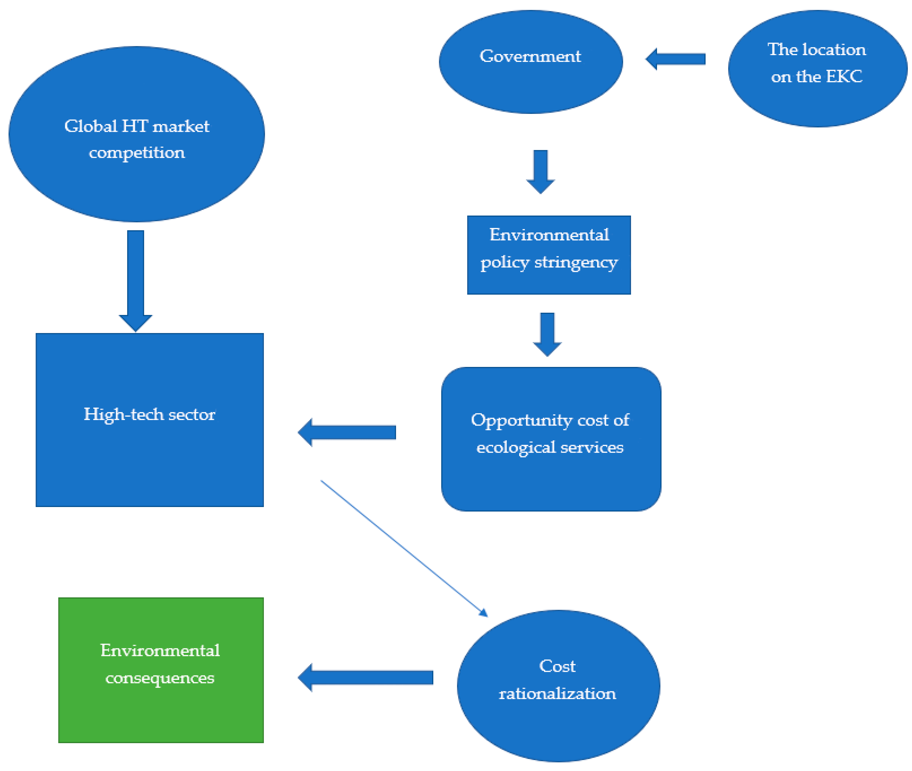Firstly, it evolves how facilitated technology dissemination and tightened environmental standards complicate securing competitiveness and make technological innovations necessary [26]. In the second step, this effect mechanism demonstrates how these technological innovations undertake a supererogatory act in green economic transformation. A conceptual framework diagram is provided in Figure 1 to provide an intuitive grasp of the study’s overall architecture and clearly illustrate the research flow.

3. Literature Review

The relationship between export competitiveness and environmental sustainability has traditionally been analyzed through a unidirectional lens, primarily examining how environmental regulations manipulate export performance [26,28,29,30]. However, our first comprehensive scan concludes that the related inverse unidirectional linkage has received little attention. While earlier studies broadly examined the environmental costs of trade liberalization, few have directly investigated how HT export competitiveness, particularly under varying policy stringency, affects environmental sustainability [31,32,33,34,35,36,37,38]. This study addresses this gap by focusing on the pattern of comparative advantages, their moderating role in cost rationalization, and the environmental outcomes resulting from this process.

In order to cease the deadlock of the current stream of literature and obtain more specific evidence about the environmental consequences of trade, researchers focused on disaggregating trade into technological intensity and sectoral identity [38,39,40,41,42,43]. According to its promising contribution to economic development, international technology spillovers, and green economic transformation [13,44], the HT industry has persuaded researchers to investigate this sector’s trade in their studies specifically [45,46,47,48]. In studies specific to a single country, manufactured HT exports have been suggested as a proxy for HT exports [46,49]. On the other side, in studies where country groups are considered, the share of medium and HT exports in total manufactured exports, HT exports in current USD, and finally, information and communication exports in total exports have been recommended as proxies for HT exports [45,47,48,49,50,51,52].

On the empirical methodology side, refs. [46,50] followed the autoregressive lag (ARDL) model in their research specific to single countries. According to the second group, which consists of cross-country studies, researchers have employed the panel two-stage least square (2SLS) instrumental variable technique like [48], the system generalized method of moments (GMM) analysis like [47], the MM-QR approach like [52], the panel ordinary least squares (OLS) estimator like [51], and dynamic common correlated panel data modeling techniques like [49].

When we classify the aforementioned studies related to their insights, many researchers suggest a positive impact of HT exports on environmental sustainability. First of all, this group of studies treats high-tech industries as core industries of industrial technology and mentions their superiority in technological innovation ability [53]. More specifically, they assert that the prioritization of the high-tech industry may facilitate the adoption and spread of green supply chain management practices, the supererogatory act of technological advancements in green innovations, and industrial structure rationalization and consequently enable better environmental conditions [46,47,48,49,54]. Nevertheless, some other studies demonstrate that prioritizing the HT industry and its leading effect on increasing exports may hinder environmental sustainability. For example, refs. [51,52] claim that maintaining HT export competitiveness necessitates industrial specialization and a particular resource allocation strategy that manages this specialization. Since HT products consist of environmentally harmful inputs, and the production process is relatively energy-intensive, the increasing market share of HT exports would escalate energy demand and cause environmental degradation.

It is pertinent to conclude that the vast majority of related research does not comprehensively dwell on the environmental outcome of HT export competitiveness. In addition, researchers have intensively chosen to select absolute HT export figures as trade-related environmental impact determinants and have neglected the dynamics of the pattern of competitiveness and its multiplying effects under different sorts of environmental policy stringency. More specifically, the environmental results of the enhancement of the HT industry have been analyzed within a narrow and static understanding. This issue first arises from the poor proxy selection for the HT industry development and the lack of consideration of competitiveness. At this point, using country-specific absolute HT export figures does not reveal an accurate comparison of countries’ global competitive positions. Therefore, benefiting from recent comparative advantage indices may provide a clear picture of countries’ relative HT industry improvements. Moreover, enabling the presence of competitiveness with suitable proxy selection offers a comprehensive evaluation of the environmental consequences of competition-induced cost rationalization and innovation strategies. Considering the degree of environmental policy stringency may sophisticate the analysis by prioritizing different components related to cost rationalization and facilitating the supererogatory act of technological advancements in green economic transformation.

The contributions of this study to the literature can be listed as follows. First, it provides a new analytical framework by integrating advanced machine learning models with the method of moments quantile regression (MM-QR) and offers the dual benefit of robust estimation and distribution-sensitive inference. Second, it improves the measurement of high-technology export competitiveness using the normalized revealed comparative advantage (NRCA) index, addressing the limitations of traditional RCA metrics and enabling more accurate cross-country comparisons. Third, the study investigates the heterogeneous environmental impact of competitiveness using quantile regression techniques, thereby identifying policy-relevant changes across levels of ecological degradation. Finally, it translates these empirical insights into differentiated policy recommendations based on countries’ environmental positions and offers applicable strategies that align competitiveness with sustainability. Collectively, these contributions fill critical gaps in the literature and provide methodological and policy-relevant advances for decision-makers.

4. Model and Data

At this stage, we suggest an empirical model in accordance with the STIRPAT framework introduced by [55,56]. This framework is intensively followed in applied ecological studies to evaluate the environmental impact mechanisms regarding various aspects. We join the vast majority of those following the STIRPAT model because this framework is competent in illustrating the outcome of behavioral factors on environmental conditions [57]. The fundamental equation of the STIRPAT model is as follows:

$$I_i=\beta P_i^x{A}_i^y{T}_i^z{\mu }_i$$

(1)

This framework exposes the fundamental I = PAT equation’s multiplicative logic, addressing anthropogenic variables: population (P), affluence (A), and technology (T) as determinants of environmental impact (I). After taking the logarithm for both sides of the equation, the initial model transforms to

$$ln{I}_{it}=\beta +x\left(ln{P}_{it}\right)+y\left(ln{A}_{it}\right)+z\left(ln{T}_{it}\right)+{\mu }_i$$

(2)

According to the last formation of the model, i refers to cross-sections; t denotes the time dimension; x, y, and z denote elasticities of environmental impact related to anthropogenic variables, respectively; $\mu$ is the stochastic error term, and $\beta$ is the constant. Within representative models, air and water pollution, land use and biodiversity, climate change, waste and circular economy, and finally, resource consumption determinants such as Ecological and Carbon Footprints have been indicated as environmental impact (I) proxies [58]. In addition, urbanization determinants have been selected as population (P), GDP determinants as affluence (A), and technological capability and innovation variables as technology (T) proxies [59]. In the empirical analysis, we extend and enrich the fundamental STIRPAT framework by the use of unique and alternative variables and try to figure out how high-tech export competitiveness affects environmental sustainability.

Table 1. Variable description.

Variable	Purpose	Source	Description
EF	Dependent variable (proxy of T)	Global footprint network	Ecological Footprint (gha per person)
URB	Independent variable (proxy of T)	https://www.footprintnetwork.org/ (accessed on 23 December 2024)	Urban population (% of total population)
GDPPC	Independent variable (proxy of T)	World Bank Database	GDP per capita (current USD)
NRCA	Independent variable (international competitiveness proxy)	https://data.worldbank.org/ (accessed on 21 December 2024)	Normalized revealed comparative advantage index [63]. The index calculations are based on Standard International Trade Classification revision 3 group 7 (machinery and equipment) data.
HC	Independent variable (proxy of T)	World Bank Database	Human capital index, based on years of schooling and returns to education
PATENT	Independent variable (proxy of T)	https://data.worldbank.org/ (accessed on 23 December 2024)	Triadic patent families (in total numbers). Set of patents registered in various countries.
KOFRTGI	Independent variable (globalization proxy)	UN Comtrade Database	Trade globalization index [64].

represents comprehensive information on each variable included in the empirical models. Among various alternative environmental impact proxies, we decide to select the variable of Ecological Footprint (EF) because this notion denotes a measure that deciphers the environmental impact of households, nations, or the world by estimating the biologically productive land and water required to compensate for resource use and absorb generated waste. In addition, EF accounting stands on professionally managed data sets issued by international organizations like the United Nations (UN) and the United Nations Food and Agriculture Organization (FAO) [60,61]. When we continue explaining the other specified variables, the share of urban population in the total population variable is selected as urbanization, GDP per capita as affluence, and patent applications and human capital accumulation as technological capability indicators. Lastly, the NRCA index proposed by [62] is used as an export competitiveness proxy, and the trade globalization index is used as a trade globalization proxy.

The extension of the STIRPAT model to include normalized revealed comparative advantage (NRCA) and trade globalization (KOFRTGI) is grounded in the interplay between trade theory and environmental economics. NRCA, as a refined measure of sectoral competitiveness, operationalizes the Ricardian principle of comparative advantage while addressing the limitations of traditional trade intensity metrics—its normalization accounts for asymmetries in market size and global demand, making it particularly suited to assess how specialized industrial capabilities (e.g., high-tech vs. traditional sectors) moderate environmental impacts. This aligns with the technique effect of trade, where competitive industries under stringent regulations tend to adopt cleaner technologies, as predicted by the Porter hypothesis. Meanwhile, the KOF trade globalization index (KOFRTGI) captures the dual role of trade openness in environmental outcomes, reflecting both the pollution haven risk (scale effect) and technology diffusion opportunities (technique effect). Its multidimensional structure—incorporating de facto trade flows and de jure policies—allows the model to disentangle whether globalization amplifies or mitigates the environmental consequences of competitiveness. Together, these variables introduce critical structural and institutional dimensions to the STIRPAT framework, testing how trade-driven specialization and integration interact with population, affluence, and technology to shape emissions trajectories. Their inclusion responds to recent calls in ecological economics to move beyond aggregate trade metrics and instead examine the contextual conditions under which competitiveness and globalization either exacerbate or alleviate environmental degradation. Finally, the reason behind this preference is NRCA’s relative accuracy in unraveling the status of comparative advantages for specific sectors, as opposed to other revealed comparative advantage indices.

To investigate the possible impact of HT export competitiveness and other anthropogenic factors on environmental sustainability, we construct a balanced data set containing annual data of fifteen G20 countries (Argentina, Brazil, Canada, China, France, Germany, India, Indonesia, Italy, Japan, Republic of Korea, Mexico, Turkiye, UK, USA). To manage a balanced panel data set and provide data consistency, we restricted the period from 1992 to 2019 and excluded five G20 countries (Australia, Russia, Saudi Arabia, South Africa, the European Union) because of data unavailability. Finally, as we manage the empirical analysis with annual data, the issue of seasonality is neglected.

The descriptive statistics of each variable are presented in

Table 2. Descriptive statistics.

	lnEF	lnURB	lnGDPPC	lnNRCA	lnHC	lnPATENT	lnKOFRTGI
Mean	19.94	4.22	9.34	0.01	0.45	5.71	3.90
Median	19.65	4.35	9.83	−0.01	0.46	6.45	3.97
Max.	22.35	4.52	11.09	0.04	0.58	9.901	4.38
Min.	18.54	3.26	5.71	−0.01	0.19	−2.30	2.95
Std. Dev.	0.88	0.32	1.35	0.01	0.10	2.87	0.30
Skew.	1.13	−1.71	−0.89	1.76	−0.50	−0.41	−0.75
Kurt.	3.59	4.76	2.84	7.31	2.17	2.14	3.04
Jarque–Bera	95.61	257.93	56.58	541.66	29.52	24.75	39.76
Prob.	0.00	0.00	0.00	0.00	0.00	0.00	0.00
Sum	8374.60	1771.81	3921.49	0.20	188.76	2398.21	1636.03
Sum Sq. Dev.	321.15	42.05	763.81	0.03	4.11	3448.05	38.29
n	420	420	420	420	420	420	420

. The initial pre-analysis depicts that all variables are right-tailed and skewed (lnEF and lnNRCA are positive, while others are negatively skewed). Moreover, the following statistics show that the variable lnNRCA is leptokurtic, and other variables are near normal. Finally, the Jarque–Bera p-values suggest that none of the variables are normally distributed. Thus, we set up a convenient empirical estimation process with data properties and use robust estimators, quantile regression, and bootstrapping to address non-normality and skewed distributions.

5. Research Questions and Hypotheses

We mentioned that the vast majority of related studies basically centered on decomposing the environmental impact mechanism of trade. The lack of strategic specification in the research topic and the recurrence of similar approaches for various samples resulted in a wide range of outcomes. To revive a new debate, this study focuses on HT-sectors’ cost rationalization strategies under pressures of global competition and national environmental policy stringency and tests the hypothesis that competition-induced technological innovation in high-tech exports exacerbates environmental degradation in G20 countries under weak regulatory pressure.

6. Estimation and Prediction Procedures

In this study, we propose a hybrid empirical framework combining econometrics’ capability to provide interpretability and causal structure and ML’s distinctive property in prediction power, as well as an illustration of complexity. The fractures of the empirical analysis serve distinct but complementary purposes, and using them in conjunction enables a much more comprehensive understanding of the linkage between predictors and the outcome variable than using either one alone. To this end, we initially classify ML regression algorithms’ prediction performances considering R², MSE, and MAE values. Secondly, we determine how much a variable affects the model regarding the prediction of best-performing algorithms. Finally, we use the method of moments bootstrap quantile regression procedures to demonstrate how predictors affect the entire distribution of the outcome, capturing varying effects across different points (heterogeneity) and being more robust to outliers.

6.1. Machine Learning Algorithms

The machine learning algorithm family has a large number of members. SVR, GP, XGBoost, and AdaBoost algorithms were used in our study. This is due to the strengths of these methods in handling non-linear, complex, and high variance data environments, which are prominent in environmental impact estimations and panel data sets in the literature. In addition, these methods provide information about the importance level of the variable. In particular, SVR and GP algorithms were preferred because they showed high performance in modeling small data sets and complex relationships. XGBoost and AdaBoost were included due to the advantages of error correction and generalizability of ensemble methods. The performances of the algorithms were evaluated according to R², MSE, and MAE criteria, and the models providing the highest accuracy were determined. Five-fold cross-validation was applied with the grid search method in the parameter optimization process, considering the hyperparameter ranges suggested in the literature for each algorithm. For example, basic parameters such as epsilon and C for SVR, kernel functions for GP, tree depth, and learning rate for XGBoost are optimized. This strategy ensures that the models produce consistent results without experiencing overfitting problems. At the same time, prediction and significance level analyses were performed with the best-performing configurations. In addition, ML models were used not alone but with Quantile Regression by Method of Moments (MM-QR). In this way, distributional heterogeneity that average-based methods can ignore was revealed. This hybrid approach provides the predictive power of ML techniques, while MM QR provides interpretability and robustness against outliers and skewness.

6.1.1. Support Vector Regression (SVR)

SVR adapts the support vector machine (SVM) algorithm to regression problems. This method aims to find the most suitable regression line within a certain tolerance range (ϵ-tube), independent of most data. SVR estimates the value of a dependent continuous variable by finding the tube that best approximates the continuous-valued function and minimizing the estimation error. SVR derives a prediction function from the data, as shown in Equation (5) uses hyper-plane logic and provides flexibility using kernel functions in non-linear problems. The fundamental kernel functions are given in Equations (3) and (4). Using kernel functions transforms data into a higher-dimensional feature space, thus enabling the modeling of non-linear relationships.

$$K\left(x_i,x_j\right)=exp\left(-\mathsf{\gamma }{\left|\right|x_i-x_j\left|\right|}^2\right)$$

(3)

$$K\left(x_i,x_j\right)={\left(x_i^T{x}_j+c\right)}^d$$

(4)

The radial basis function (RBF) given by Equation (3) is the most commonly used kernel and has a distinctive feature of performing well in non-linear problems. The polynomial kernel given by Equation (4) is suitable for modeling non-linear and polynomial relationships. While SVR minimizes the error between the values estimated using Equation (5) and the real values by Equation (6), it also aims to preserve the model’s generalization ability.

$$f\left(x\right)=w^T\mathsf{\varphi }\left(x\right)+b$$

(5)

In Equation (5), x, $\varphi \left(x\right)$, w, and b depict the feature space transformation with kernel function, weight vector, and side term in the model. When creating the prediction function, the aim is to keep the errors within a certain tolerance (ϵ). Unlike traditional methods, SVR focuses on errors that exceed the tolerance limit rather than the magnitude of the errors. SVR uses an ε-insensitive loss function that penalizes estimates further than ε from the desired output. Different loss functions can be used, such as linear or quadratic. The value of ε determines the width of the tube. The optimization problem is defined as follows:

$$\begin{gathered} min{\displaystyle \frac{1}{2}}{\left|\right|w\left|\right|}^2+C\sum _{i=1}^n\left({\mathsf{\xi }}_i+{\mathsf{\xi }}_1^{*}\right) \\ \mathrm{s}.\mathrm{t}. \\ {y}_i-\left(w^T\mathsf{\varphi }\left(x_i\right)+b\right)\le \mathsf{ϵ}+{\mathsf{\xi }}_i \\ \left(w^T\varphi \left(x_i\right)+b\right)-{\mathrm{y}}_{\mathrm{i}}\le ϵ+{\xi }_i^{*} \\ {\xi }_i,{\mathsf{\xi }}_i^{*}\ge 0 \end{gathered}$$

(6)

According to Equation (6) ${\xi }_i$ and ${\xi }_i^{*}$, $ϵ$ and C mean slack variables, tolerance range, and regularization parameter, respectively. The regularization parameter controls the balance between the model’s flexibility and its ability to generalize.

6.1.2. Gaussian Processes (GP)

A Gaussian process is a process in which the means and covariances of a set of random variables have a Gaussian distribution. A GP is defined as

$$f\left(x\right)~GP\left(m\left(x\right),k\left(x,x^{\prime }\right)\right)$$

(7)

In Equation (7), $f\left(x\right)$ is the function modeled by the GP, $m\left(x\right)$ is the mean function, and finally $k\left(x,x^{\prime }\right)$ is the covariance (kernel) function determining the relationship between two points. The mean function is usually taken as zero ($m\left(x\right)=0)$, only when the covariance structure is used. The covariance function is at the core of GP. This function defines the similarity or dependency between two input points. Some common covariance functions (radial basis function (RBF), linear, and Matérn) are explained through the following equations:

$$k\left(x,x^{\prime }\right)={\mathsf{\sigma }}_f^{2}exp\left(-{\displaystyle \frac{{\left|\right|x-x^{\prime }\left|\right|}^2}{2l^2}}\right)$$

(8)

The RBF and linear kernels are exposed in Equations (8) and (9). In this equation, l represents the scaling parameter, and ${\sigma }_f$ represents the variance of the function.

$$k\left(x,x^{\prime }\right)=x^T{x}^{\prime }$$

(9)

Matérn kernels are general forms of RBF. An additional parameter v controls the smoothness of the resulting function. The approximated function becomes smoother when the value v becomes smaller. As $v\to \infty$, the kernel becomes equivalent to the RBF kernel. When v = 0.5, the Matérn kernel becomes identical to the absolute exponential kernel. The kernel is given by

$$k\left(x,x^{\prime }\right)={\displaystyle \frac{1}{\Gamma \left(v\right)2^{v-1}}}{\left({\displaystyle \frac{\sqrt{2v}}{l}}d\left(x,x^{\prime }\right)\right)}^v{K}_v\left({\displaystyle \frac{\sqrt{2v}}{l}}d\left(x,x^{\prime }\right)\right)$$

(10)

where d is the Euclidean distance, $K_v$ is a modified Bessel function and $\Gamma \left(v\right)$ is the gamma function. Kernel selection can significantly affect the accuracy of the model. In GP, the expected value and variance for x are given in Equations (11) and (12), respectively.

$$\mathsf{\mu }\left(x_{\ast }\right)=k_{\ast }^T{\left(K+{\mathsf{\sigma }}_n^{2}l\right)}^{-1}c$$

(11)

$${\mathsf{\sigma }}^2\left(x_{\ast }\right)=k\left(x_{\ast },x_{\ast }\right)-k_{\ast }^T{ \left(K+{\sigma }_n^{2}l\right)}^{-1}{k}_{\ast }$$

(12)

Here, $k_{\ast }$ represents the covariance of the test and training points, K represents the covariance matrix of the training points, and ${\sigma }_n^2$ represents the noise variance.

6.1.3. Extreme Gradient Boosting (XGBoost)

XGBoost is an optimized and faster version of the gradient boosting algorithm. It is a learning algorithm that iteratively builds decision trees and minimizes the error at each step. The method performs error minimization by training learners sequentially and correcting the errors of the previous model at each step. It works effectively in both classification and regression problems. The model is formulated as follows:

$$y_i={\sum }_{k=1}^K{f}_k\left(x_i\right)+\mathsf{ϵ}$$

(13)

In this function, $y_i$ represents the target variable, $x_i$ implies the input features, $f_k\left(x\right)$ the function learned by each decision tree, and K represents the total number of trees. These functions are learned with the optimization problem in Equation (14).

$$Min L\left(\mathsf{\Theta }\right)+{\sum }_{k=1}^K\mathsf{\Omega }\left(f_k\right)$$

(14)

In this equation, $\Omega \left(f_k\right)=\gamma T+{\displaystyle \frac{1}{2}}\lambda {\left|\right|w\left|\right|}^2$ represents the complexity penalty of trees, $\gamma$ and $\lambda$ are the regularization parameters, and $L\left(\Theta \right)$ is the estimation error.

6.1.4. Adaptive Boosting (AdaBoost)

AdaBoost is a boosting method that creates a strong prediction model using weak learners like decision trees. It updates the weights of the weak learners in each iteration by following their errors. In this way, the model performance is increased by focusing more on the errors. The basic approach of AdaBoost is to train each weak learner by giving more weight to the misclassified data at each step. Thus, the focus is on correcting the errors of the weak learners and creating a strong ensemble model. AdaBoost creates weak learners in an iterative process. In each iteration, we have the following: (i) Weighting of Errors: Each data point is assigned a weight according to the error made in that iteration. The weight of incorrectly classified data increases and that of correctly classified data decreases. (ii) Training of New Learner: A new learner is trained on the weighted data set. (iii) Updating the Ensemble Model: The new learner is added to the ensemble, which is repeated to strengthen the model. The weight (${\alpha }_t$) of each weak learner is calculated as

$${\mathsf{\alpha }}_t={\displaystyle \frac{1}{2}}ln\left({\displaystyle \frac{1-e_t}{e_t}}\right)$$

(15)

Here, $e_t$ is the error rate of the tth weak learner. While the influence of weak learners with large error rates decreases in the population, those with low errors gain more weight. After learning, the final classifier is based on a linear combination of the weak classifiers.

$$H\left(x\right)=sign\left(\sum _{t=1}^T{\mathsf{\alpha }}_t{h}_t\left(x\right)\right)$$

(16)

Here, $h_t\left(x\right)$ is the output of the tth weak learner.

6.2. Method of Moments Quantile Regression (MM-QR)

The quantile regression equation is defined as in Equation (17).

$$Q_Y\left(\mathsf{\tau }|X\right)=X^T\mathsf{\beta }\left(\mathsf{\tau }\right)$$

(17)

This equation expresses the $\tau$^th quartile of Y when X is given ($\tau =0.25, 0.50, 0.75$). Where X is the independent variable vector and $\beta \left(\tau \right)$ is the coefficient vector to be estimated for the $\tau$^th quantile. Quantile regression minimizes Equation (18) instead of minimizing the sum of error squares as in classical OLS.

$$\widehat{\beta }(\tau )=arg\underset{\mathsf{\beta }}{\mathrm{m}\mathrm{i}\mathrm{n}}\sum _{i=1}^n{\rho }_{\tau }\left(y_i-x_i^T\beta \right)$$

(18)

Here, ${\rho }_{\tau }\left(u\right)$ is defined as the asymmetric absolute error function $\left({\rho }_{\mathsf{\tau }}\left(u\right)=u\left(\tau -I\left(u<0\right)\right)\right)$, and I is an indicator function. This study uses [63] MM-QR and BS-QR approaches for parameter estimation. MM-QR assumes a conditional location-scale structure. Therefore, the model given in Equation (15) is defined as in Equation (19).

$$Y_i=X_i^{\top }\mathsf{\beta }+\mathsf{\sigma }\left(X_i\right)u_i$$

(19)

Here, $\beta$, $\sigma \left(X_i\right)$, and $u_i$ are the location parameter, the scale function, and the standardized error term, respectively. The goal of this approach is to estimate the first moment given in Equation (20). However, since the check function (derivative of the quantile loss function, ${\psi }_{\tau }\left(u\right)=\tau -I\left(u<0\right)$) in the equation is not differentiable, parameter estimation is executed using iterative methods.

$$E\left[{\mathsf{\psi }}_{\tau }\left({\displaystyle \frac{Y_i-X_i^{\top }\mathsf{\beta }}{\mathsf{\sigma }\left(X_i\right)}}\right)\cdot Z_i\right]=0$$

(20)

While MM-QR estimates the parameters more flexibly and sensitively to heteroskedasticity using moments within the conditional distribution, BS-QR estimates the parameters by purifying the bias values originating from the sample by resampling.

7. Results

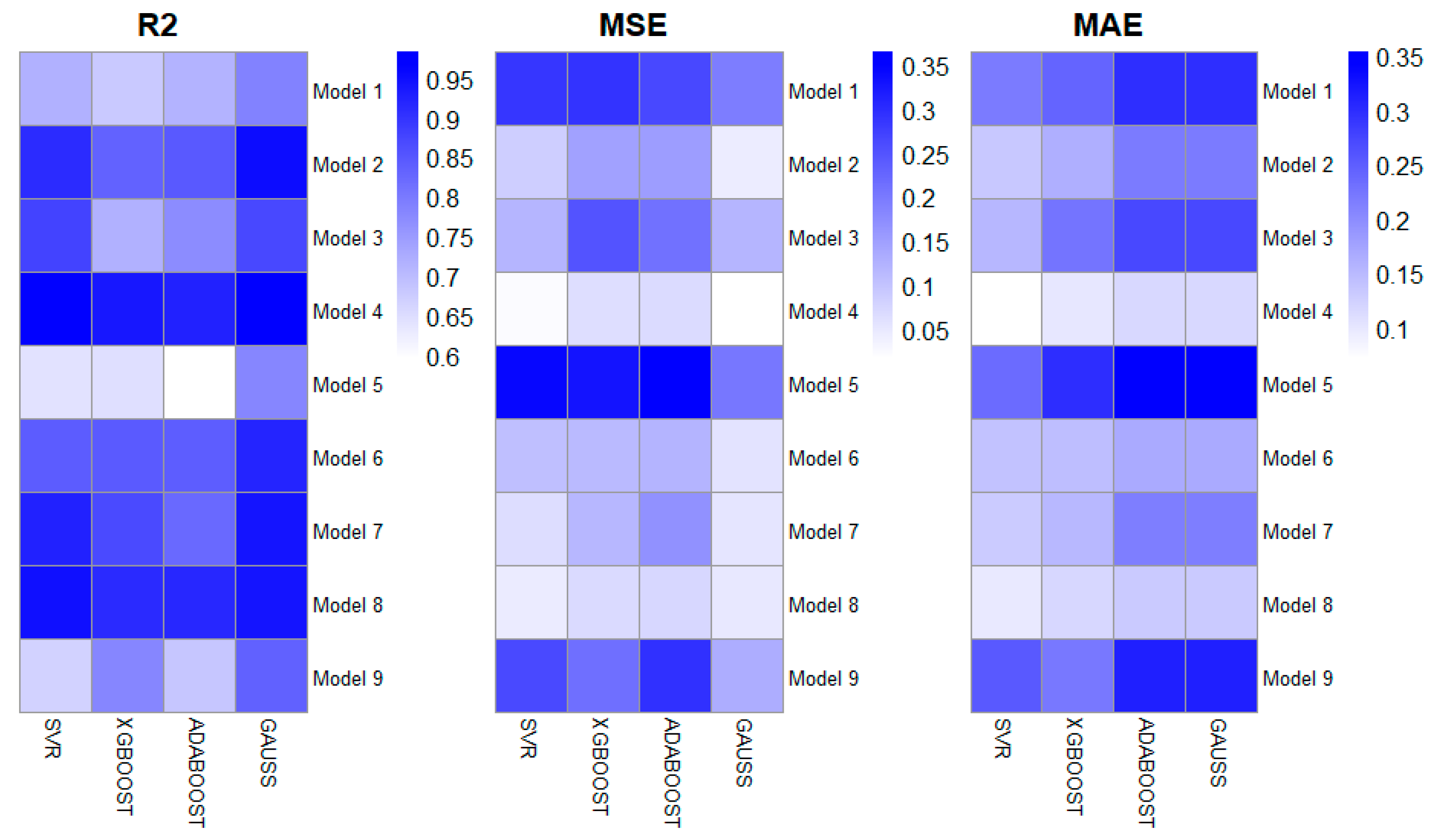
In the initial step of the empirical analysis,

Table 3. Comparison of the ML algorithms.

	SVR			XGBOOST			ADABOOST			GAUSS
Models	R2	MSE	MAE	R2	MSE	MAE	R2	MSE	MAE	R2	MSE	MAE
(I)	0.7168	0.2865	0.2179	0.6798	0.2898	0.2426	0.7143	0.2651	0.2977	0.7859 *	0.1952 *	0.2977 *
(II)	0.9110	0.0847	0.1329	0.8343	0.1477	0.1608	0.8465	0.1514	0.2186	0.9524 *	0.0440 *	0.2186 *
(III)	0.8772 *	0.1189 *	0.1526 *	0.7168	0.2492	0.2257	0.7719	0.2121	0.2720	0.8722	0.1185	0.2720
(IV)	0.9760	0.0225	0.0719	0.9382	0.0630	0.0991	0.9239	0.0675	0.1151	0.9830 *	0.0172 *	0.1151 *
(V)	0.6414	0.3454	0.2340	0.6455	0.3288	0.2989	0.5963	0.3647	0.3533	0.7808 *	0.2034 *	0.3533 *
(VI)	0.8421	0.1053	0.1399	0.8454	0.1125	0.1444	0.8406	0.1217	0.1668	0.9200 *	0.0563 *	0.1668 *
(VII)	0.9242	0.0643	0.1299	0.8691	0.1160	0.1515	0.8227	0.1678	0.2145	0.9420 *	0.0535 *	0.2145 *
(VIII)	0.9485 *	0.0453 *	0.0974 *	0.9118	0.0683	0.1170	0.9162	0.0726	0.1306	0.9416	0.0495	0.1306
(IX)	0.6653	0.2639	0.2550	0.7808	0.2142	0.2217	0.6831	0.2939	0.3127	0.8353 *	0.1314 *	0.3127 *

Note: The best ML algorithms for the evaluated models are marked with *.

and Figure 2 imply and visualize ML regression algorithms’ prediction performances due to R², MSE, and MAE values. According to the related analysis, the SVR is the best approach for models III and VIII, while the GP is the best for all other models. In addition, Figure 2 contains heatmaps created for three evaluation metrics (R², MSE, MAS), respectively. The darker colors in the heatmap prepared for R² correspond to higher R² values and, therefore, to the model’s explanatory power. The lighter colors in the other two heatmaps correspond to the errors in the model, that is, the reliability of the models. On the other side,

Table 4. Importance levels and ratio (%) of independent variables.

	Dependent Variable: lnEF
	Models
Independent Variables	(I)	(II)	(III)	(IV)	(V)	(VI)	(VII)	(VIII)	(IX)
lnURB	0.7134	0.6886	0.8716	0.6618	1.0449 *	0.8250	1.0284 *	1.4357	1.0060
	(0.30)	(0.23)	(0.29)	(0.25)	(0.43)	(0.31)	(0.34)	(0.21)	(0.34)
lnGDPPC	0.6212	0.7014	0.6307	0.3194	0.6270	0.6179	0.5152	1.5187	0.9097
	(0.26)	(0.23)	(0.21)	(0.12)	(0.26)	(0.24)	(0.17)	(0.22)	(0.31)
lnNRCA	1.0785 *	0.9163 *	0.9804 *	0.8241 *
	(0.44)	(0.30)	(0.32)	(0.32)
lnHC			0.5661		0.7600		0.7022
			(0.18)		(0.31)		(0.23)
lnPATENT				0.8093		1.2012 *		3.2458 *
				(0.31)		(0.45)		(0.48)
lnKOFTRGI		0.7227					0.8088	0.5899	1.0200 *
		(0.24)					(0.26)	(0.09)	(0.35)

Notes: The importance ratios are given in parentheses. * indicates the variable with the relatively highest importance level.

illustrates the importance levels of the independent variables in the best ML algorithms according to Table 3. The importance level measures the contribution of each independent variable to the model in ML algorithms. In other words, it tells how much a variable affects the model in terms of prediction. Removing high values from the model can seriously reduce its success. In the opposite case, variables with low importance do not affect the model’s prediction success much, and it can even be said that they can be removed from the model. The values in Table 4 express the importance levels. The values given in parentheses are the importance ratio. No variable with a low importance level exists in all our proposed models. This is an indicator of the accuracy of the proposed models. At the same time, the difference between the highest and lowest importance levels for any model is relatively small. In this case, the variables used are almost equally important to the model’s success. Only for Model (VIII), the lnKOFTRGI value has a relatively low significance rate of 0.09. Lastly, the relatively best-performing ML algorithms imply that small changes in lnNRCA consistently lead to relatively significant changes in the related model’s prediction. This outcome signifies that HT export competitiveness has a dominant influence on the model’s output.

Table 5. MM-QR estimation results.

		Dependent Variable: lnEF
		Models
Independent Variables	Quantiles	(I)	(II)	(III)	(IV)	(V)	(VI)	(VII)	(VIII)	(IX)
lnURB	0.25	−2.13 ***	−2.14 ***	−2.25 ***	−0.77	−2.13 ***	−0.70 ***	−2.35 ***	−0.89 ***	−2.21 ***
		(0.08)	(0.19)	(0.08)	(18.26)	(0.10)	(0.12)	(0.29)	(0.16)	(0.18)
	0.50	−2.24 ***	−2.50 ***	−2.25 ***	−0.59	−2.18 ***	−0.54 **	−2.60 ***	−0.90 *	−2.65 ***
		(0.11)	(0.22)	(0.11)	(14.97)	(0.13)	(0.26)	(0.28)	(0.50)	(0.21)
	0.75	−2.42 ***	−3.12 ***	−2.31 ***	−0.06	−2.30 ***	−0.11	−3.18 ***	−0.94	−3.42 ***
		(0.23)	(0.37)	(0.22)	(4.93)	(0.27)	(1.02)	(0.37)	(2.30)	(0.40)
lnGDPPC	0.25	0.30 ***	0.32 ***	0.25 ***	−0.23	0.24 ***	−0.25 ***	0.34 ***	−0.15 ***	0.41 ***
		(0.01)	(0.04)	(0.03)	(5.50)	(0.04)	(0.03)	(0.09)	(0.05)	(0.04)
	0.50	0.31 ***	0.43 ***	0.22 ***	−0.33	0.21 ***	−0.34 ***	0.39 ***	−0.18	0.54 ***
		(0.02)	(0.05)	(0.04)	(4.51)	(0.05)	(0.08)	(0.08)	(0.15)	(0.05)
	0.75	0.34 ***	0.64 ***	0.16 *	−0.62	0.16	−0.61 *	0.47 ***	−0.29	0.78 ***
		(0.05)	(0.09)	(0.09)	(1.48)	(0.10)	(0.31)	(0.11)	(0.71)	(0.10)
lnNRCA	0.25	25.74 ***	21.86 ***	24.90 ***	4.76
		(1.84)	(4.23)	(1.91)	(355.67)
	0.50	25.07 ***	20.08 ***	24.20 ***	2.65
		(2.60)	(4.61)	(2.59)	(291.68)
	0.75	23.91 ***	16.92 ***	22.91 ***	−3.85
		(4.94)	(6.91)	(4.97)	(96.08)
lnHC	0.25			0.93 ***		1.46 ***		1.33 *
				(0.35)		(0.42)		(0.75)
	0.50			1.49 ***		1.96 ***		2.29 ***
				(0.48)		(0.54)		(0.71)
	0.75			2.55 **		3.27 ***		4.03 ***
				(4.97)		(1.13)		(0.96)
lnPATENT	0.25				0.20		0.21 ***		0.21 ***
					(1.45)		(0.01)		(0.01)
	0.50				0.24		0.25 ***		0.24 ***
					(1.19)		(0.02)		(0.03)
	0.75				0.37		0.37 ***		0.33 **
					(0.39)		(0.08)		(0.15)
lnKOFTRGI	0.25		−0.04					−0.24	−0.33 ***	−0.27 *
			(0.14)					(0.21)	(0.31)	(0.14)
	0.50		−0.43 ***					−0.71 ***	−0.48	−0.72 ***
			(0.16)					(0.20)	(0.31)	(0.16)
	0.75		−1.12 ***					−1.56 ***	−0.97	−1.51 ***
			(0.31)					(0.32)	(1.42)	(0.32)

Notes: ***, **, and * indicate 1%, 5%, and 10% level of significance, respectively. Robust standard errors are in parentheses.

and

Table 6. BS-QR estimation results.

		Dependent Variable: lnEF
		Models
Independent Variables	Quantiles	(I)	(II)	(III)	(IV)	(V)	(VI)	(VII)	(VIII)	(IX)
lnURB	0.25	−2.26 ***	−2.39 ***	−2.28 ***	−1.21 ***	−2.26 ***	−1.15 ***	−2.29 ***	−1.22 ***	−2.22 ***
		(0.09)	(0.14)	(0.07)	(0.12)	(0.13)	(0.14)	(0.15)	(0.14)	(0.17)
	0.50	−2.17 ***	−2.56 ***	−2.24 ***	−0.58 ***	−2.28 ***	−0.33*	−2.85 ***	−0.86 ***	−2.67 ***
		(0.16)	(0.28)	(0.17)	(0.19)	(0.21)	(0.19)	(0.26)	(0.18)	(0.24)
	0.75	−1.34 ***	−3.18 ***	−1.15 *	−0.01	−1.59 ***	−0.07	−2.58 ***	−1.28 **	−3.05 ***
		(0.65)	(0.52)	(0.68)	(0.34)	(0.52)	(0.30)	(0.34)	(0.57)	(0.60)
lnGDPPC	0.25	0.35 ***	0.39 ***	0.27 ***	−0.05	0.23 ***	−0.07	0.28 ***	−0.01	0.38 ***
		(0.22)	(0.03)	(0.02)	(0.04)	(0.04)	(0.04)	(0.05)	(0.04)	(0.04)
	0.50	0.28 ***	0.43 ***	0.24 ***	−0.31 ***	0.26 ***	−0.40 ***	0.45 ***	−0.20 ***	0.51 ***
		(0.33)	(0.07)	(0.05)	(0.08)	(0.06)	(0.07)	(0.05)	(0.05)	(0.04)
	0.75	−0.09	0.63 ***	−0.30	−0.68 ***	−0.24	−0.65 ***	0.33 ***	−0.25	0.67 ***
		(0.16)	(0.12)	(0.19)	(0.09)	(0.15)	(0.08)	(0.09)	(0.16)	(0.12)
lnNRCA	0.25	19.47 ***	19.49 ***	19.18 ***	10.70 ***
		(2.43)	(2.49)	(1.87)	(1.48)
	0.50	25.48 ***	22.03 ***	25.33 ***	9.99 ***
		(3.66)	(4.55)	(4.36)	(2.02)
	0.75	32.19 ***	17.56	28.09 **	−0.42
		(9.09)	(11.20)	(10.85)	(7.26)
lnHC	0.25			1.20 ***		1.93 ***		1.79 ***
				(0.28)		(0.48)		(0.40)
	0.50			0.66		1.23 *		1.85 ***
				(0.65)		(0.64)		(0.41)
	0.75			2.84		6.76 ***		4.71 ***
				(2.22)		(2.59)		(0.46)
lnPATENT	0.25				0.15 ***		0.16 ***		0.17 ***
					(0.01)		(0.01)		(0.01)
	0.50				0.19 ***		0.23 ***		0.21 ***
					(0.01)		(0.01)		(0.01)
	0.75				0.30 ***		0.29 ***		0.26 ***
					(0.04)		(0.04)		(0.05)
lnKOFTRGI	0.25		−0.11 *					−0.17 **	−0.23 **	−0.15 **
			(0.66)					(0.44)	(0.45)	(0.07)
	0.50		−0.51 **					−0.92 ***	−0.55 ***	−0.79 ***
			(0.22)					(0.13)	(0.08)	(0.14)
	0.75		−2.00 ***					−2.28 ***	−1.12 ***	−1.93 ***
			(0.32)					(0.23)	(0.36)	(0.32)

Notes: ***, **, and * indicate 1%, 5%, and 10% level of significance, respectively. Bootstrap probability values were obtained from a 250-replication distribution. Robust standard errors are in parentheses.

demonstrate the MM-QR and BS-QR results of the impact of anthropogenic factors on environmental sustainability, respectively. The parameter estimations shed light on the negative and statistically significant heterogeneous relationship between URB and EF.

The detection of heterogeneity implies that the estimated associations change at different levels of environmental degradation. Therefore, the impact of urbanization is more profound on high levels of environmental degradation than on low levels. The estimated overall positive impact of urbanization on environmental quality is consistent with previous studies [65,66,67], supporting the pivotal role of urbanization in green economic transformation. More specifically, the increasing levels of urbanization may accompany income growth, human capital accumulation, socio-cultural development, and the desire for better environmental conditions, ultimately leading to widespread environmentally friendly practices in all aspects of urban life.

The parameter estimation results indicate a positive and statistically significant linkage between GDP per capita and EF. Unlike the previous insights about heterogeneity regarding different levels of environmental degradation, the increase in GDP per capita does not lead to distinguishable effects for different quantiles. Nevertheless, the undesired ecological impact of economic development confirms the general conclusion that economic growth induces anthropogenic activities by stimulating various economic interactions [68]. Given that the coefficient for lnGDPPC is positive and statistically significant across most quantiles (Table 5 and Table 6), it is evident that economic growth, during the analyzed period, has not translated into environmental improvements among G20 countries. Moreover, it is evident that economic growth during the analyzed period has not translated into environmental improvements among G20 countries. Regarding the association between HT export competitiveness and environmental degradation, the quantile regression results indicate a positive relationship between these two variables for all quantiles. This interaction aligns with the observations of [51,52], which suggest that the G20 countries’ pursuit of extending their HT export market share involves a cost rationalization strategy that overlooks environmental sustainability considerations. In other words, considering the high dependence of the HT sector on harmful inputs and its relatively energy-intensive production process, enhancing comparative advantage in this sector may trigger increased energy demand and worsen environmental conditions.

Following the initial stream of empirical evidence, the quantile regression analysis suggests a positive and statistically significant relationship between the technological capability variables HC, PATENT, and EF. Additionally, although there is no significant gradual change in the positive association between patent applications and environmental degradation, a heterogeneous structure is evident in the linkage between human capital accumulation and environmental degradation. Similar to the environmental impact of urbanization, the environmental consequences of human capital accumulation are more profound at high levels of environmental degradation than at low levels. This insight suggests that enhancing technological capabilities may stimulate industrialization and economic growth, leading to increased resource extraction, which supports the previous suggestions of [69,70]. On the other hand, the higher environmental impact of human capital accumulation in excessive ecological degradation levels suggests that advanced R&D and technological improvements can prioritize profit-driven innovation over sustainable devices. Finally, the KOFTRGI coefficient yields a negative heterogeneous estimator, respectively. This estimation depicts that the impact of trade globalization is more profound on high levels of environmental degradation than on low levels. In line with the studies [71,72,73], trade globalization may enhance global environmental sustainability awareness and enable stringent environmental requirements for importers and exporters. This development can facilitate the rapid adoption of green technologies, leading to significant changes in regions with high levels of environmental pollution. The multiple graphs derived from the BS-QR analysis are given in Figure 3.

8. Conclusions

8.1. Discussion and Policy Implications

The WHO association between HT export competitiveness and environmental sustainability presents a delicate balance, where competition-induced factors such as cost rationalization and innovation incentives exert opposing pressures on this relationship [23]. While this study identifies a dominant trend where HT export competitiveness exacerbates environmental degradation in the G20, this outcome is not inevitable. The key determinant lies in how opportunity costs linked to environmental inputs are internalized within production processes. Crucially, our findings suggest that, in most cases, HT sectors prioritize short-term cost efficiency over ecological considerations, while environmental regulations fail to incentivize green industrial restructuring or innovation sufficiently as also demonstrated in the studies by [51,52] which found that in energy-intensive sectors, environmental regulation does not automatically lead to sustainable innovation. However, this trend is not universal. For instance, Germany and South Korea—despite their high levels of HT export competitiveness—have decoupled environmental degradation from sectoral growth through stringent regulations and targeted green industrial policies [9]. These countries demonstrate that coupling HT competitiveness with circular production standards, renewable energy integration, and green R&D subsidies can mitigate ecological harm. Similarly, Japan’s “Superior Energy Performance” program highlights how mandatory energy efficiency benchmarks in HT manufacturing can align competitiveness with sustainability. These exceptions underscore the moderating role of policy frameworks in shaping environmental outcomes.

To reconcile HT export competitiveness with environmental goals, we propose a set of policy recommendations. Firstly, governments should incentivize HT firms to adopt renewable energy, energy-efficient technologies, and circular production models. For instance, governments can implement subsidies for low-cost energy storage and apply tax breaks for green R&D to facilitate this transformation. Secondly, the World Trade Organization (WTO) should facilitate relaxed intellectual property rights (IPRs) for green technologies, particularly for developing economies, while enforcing sustainability standards in trade agreements to prevent “greenwashing.” Finally, policymakers can follow differentiated regulatory approaches and tailor environmental stringency to sectoral realities. For example, carbon pricing for energy-intensive HT subsectors could be paired with innovation grants for clean production methods.

In addition to these general conclusions, we present layered policy recommendations for country groups with different levels of environmental degradation:

For countries in the upper quantile (countries under high ecological stress (Q > 0.75)), under the heading of urgent and mandatory interventions, we recommend the following:

Public support provided to high-technology sectors should be made conditional on environmental criteria. Mandatory green R&D spending rates should be determined and monitored. Environmental taxation should be integrated into HT’s competitive strategies. Export advantages should be created for companies that produce environmentally sensitive products. For countries in the middle quantile (countries under medium environmental stress (0.25 < Q < 0.75)), under the heading of measures to accelerate the transformation process, we recommend the following:

Access to green financing (e.g., sustainability bonds) should be facilitated to increase the momentum of the green transformation. Financial support and priority should be provided to companies that produce low-carbon products. Preparations should be made for foreign trade mechanisms such as carbon border adjustment. For countries in the lower quantile (i.e., countries with relatively low environmental degradation (Q < 0.25)), under the heading of early-stage preventive policies, we recommend the following:

Investment should be made in green innovation infrastructure at an early stage. Sustainable product design (eco-design) and production models should be encouraged. Technology development strategies should be shaped with environmental principles before environmental risks emerge. In addition, considering the asymmetries depending on the level of development, we recommend that developed countries focus on green innovation leadership and diffusion, and emerging economies focus on technology transfer, harmonization of environmental standards, and institutional capacity development programs. This approach will help ensure convergence in sustainable competitiveness.

8.2. Limitations and Future Research

This study may have shortcomings that future studies should consider and address. First, although the predictions from this result do not distinguish significantly across a range of different regression specifications based on panel data analysis with heterogeneous dynamics, their consistency should be treated with caution, as the results of long-run predictions may vary across other estimation procedures. Therefore, one possible way to ensure the generalizability of the negative nexus between HT export competitiveness and environmental quality is to conduct an additional empirical analysis based on a larger sample of countries. Second, we suggest that global competition in the HT export market triggers a cost rationalization strategy that can be characterized as irresponsible in terms of environmental concerns. Advanced microeconomic studies should approach this transmission mechanism with caution for different sectors. These are potential avenues awaiting to be discussed in future studies.