Multi-Scale Ecosystem Service Supply–Demand Dynamics and Driving Mechanisms in Mainland China During the Last Two Decades: Implications for Sustainable Development

Abstract

The growing mismatch between ecosystem service (ES) supply and demand underscores the importance of thoroughly understanding their spatiotemporal patterns and key drivers to promote ecological civilization and sustainable development at the regional level in China. This study investigates six key ES indicators across mainland China—habitat quality (HQ), carbon sequestration (CS), water yield (WY), sediment delivery ratio (SDR), food production (FP), and nutrient delivery ratio (NDR)—by integrating a suite of analytical approaches. These include a spatiotemporal analysis of trade-offs and synergies in supply, demand, and their ratios; self-organizing maps (SOM) for bundle identification; and interpretable machine learning models. While prior research studies have typically examined ES at a single spatial scale, focusing on supply-side bundles or associated drivers, they have often overlooked demand dynamics and cross-scale interactions. In contrast, this study integrates SOM and SHAP-based machine learning into a dual-scale framework (grid and city levels), enabling more precise identification of scale-dependent drivers and a deeper understanding of the complex interrelationships between ES supply, demand, and their spatial mismatches. The results reveal pronounced spatiotemporal heterogeneity in ES supply and demand at both grid and city scales. Overall, the supply services display a spatial pattern of higher values in the east and south, and lower values in the west and north. High-value areas for multiple demand services are concentrated in the densely populated eastern regions. The grid scale better captures spatial clustering, enhancing the detection of trade-offs and synergies. For instance, the correlation between HQ and NDR supply increased from 0.62 (grid scale) to 0.92 (city scale), while the correlation between HQ and SDR demand decreased from −0.03 to −0.58, indicating that upscaling may highlight broader synergistic or conflicting trends missed at finer resolutions. In the spatiotemporal interaction network of supply–demand ratios, CS, WY, FP, and NDR persistently show low values (below −0.5) in western and northern regions, indicating ongoing mismatches and uneven development. Driver analysis demonstrates scale-dependent effects: at the grid scale, HQ and FP are predominantly influenced by socioeconomic factors, SDR and WY by ecological variables, and CS and NDR by climatic conditions. At the city level, socioeconomic drivers dominate most services. Based on these findings, nine distinct supply–demand bundles were identified at both scales. The largest bundle at the grid scale (B3) occupies 29.1% of the study area, while the largest city-scale bundle (B8) covers 26.5%. This study deepens the understanding of trade-offs, synergies, and driving mechanisms of ecosystem services across multiple spatial scales; reveals scale-sensitive patterns of spatial mismatch; and provides scientific support for tiered ecological compensation, integrated regional planning, and sustainable development strategies.

1. Introduction

Ecosystem services (ES) encompass a wide range of benefits provided by natural ecosystems, including provisioning, regulating, supporting, and cultural services [1,2]. Driven by rapid population growth and economic development, mismatches between ES supply and demand have become increasingly severe worldwide, particularly in mainland China [3,4]. Although national initiatives such as ecological redlines, the Grain for Green program, and large-scale restoration projects have achieved notable ecological gains—such as reducing natural forest logging by approximately 332 million cubic meters—many regions remain ecologically fragile, with persistent ES imbalances. This underscores the urgent need for accurately evaluating ES dynamics to advance ecological civilization and sustainable regional development in China.

Understanding the evolution of ES supply–demand relationships is fundamental to effective sustainable management [5,6,7]. Most existing studies apply quantitative methods—such as correlation analysis [8,9], Bayesian networks [10], and root mean square error [11]—to explore ES trade-offs and synergies, or use spatial methods like geographically weighted regression [12] and bivariate spatial autocorrelation [13] to examine spatial patterns. While supply-side interactions among ES have been widely studied, demand-side processes and integrated analyses of supply–demand interactions remain relatively neglected. Given ongoing urbanization and climate change, comprehensive analyses of how supply, demand, and their interactions shape regional sustainability are increasingly important [14,15].

Recently, scholars have started examining ES supply–demand dynamics across varied spatial scales, including watershed, regional, and urban agglomeration levels [16,17]. However, most analyses still emphasize supply-side ES, neglecting demand-side processes and comprehensive interactions between supply and demand [15,18]. Significant research has also investigated trade-offs and synergies among ES, revealing considerable spatial heterogeneity. However, how these relationships vary across scales or influence supply–demand ratios remains inadequately studied [19,20,21].

Machine learning methods, including Random Forest (RF), Support Vector Machines (SVM), and eXtreme Gradient Boosting (XGBoost), have increasingly been applied to ES modeling and driver identification [22,23,24]. Nonetheless, existing studies often rely on a single machine learning algorithm, limiting model generalizability and robustness. Additionally, analyses are typically conducted at a single spatial scale, overlooking cross-scale interactions. Moreover, the interpretability of machine learning models to reveal underlying mechanisms has rarely been prioritized. By selecting an optimal model through comparative analysis and integrating interpretable algorithms such as Shapley Additive Explanations (SHAP), these limitations can be addressed, allowing for deeper exploration of scale-dependent drivers and spatial interactions of ES supply and demand [25,26,27].

Previous research has shown that scale effects significantly influence ES supply–demand outcomes, with interactions varying across different spatial scales [18,28,29]. Hence, we hypothesize that ES supply, demand, and their ratio exhibit spatiotemporal heterogeneity across scales, and that trade-offs, synergies, and driving mechanisms differ between grid and city scales. To systematically test these hypotheses, this study integrates Self-Organizing Maps (SOM) and SHAP-based machine learning into a dual-scale (grid and city) analytical framework. Specifically, our objectives are (1) to assess spatiotemporal heterogeneity of ES supply, demand, and their interactions; (2) examine trade-offs and synergies across scales; (3) identify representative ES supply–demand bundles; (4) analyze drivers of supply–demand ratios using remote sensing data and interpretable ML; and (5) propose scale-specific spatial management strategies to support sustainable ecosystem governance. The remainder of this paper is structured as follows: Section 2 describes the study area, data sources, and methods; Section 3 presents the results; Section 4 discusses the implications; and Section 5 concludes with key insights and policy recommendations.

2. Data and Methods

2.1. Study Area and Data Sources

This study targets mainland China, with Taiwan and the Nansha Islands excluded. The region presents highly diverse and complex terrain, transitioning from eastern plains to western plateaus and mountainous areas. Due to variations in elevation, topography, and latitude, the climate exhibits distinct spatial patterns (Figure 1). Over the last twenty years, mainland China has undergone rapid economic expansion, marked by intensifying industrialization and urbanization, especially within coastal economic hubs such as the Yangtze River Delta, Pearl River Delta, and the Beijing–Tianjin–Hebei area. These regions have seen substantial growth in high-tech sectors, sharp rises in urban population, and ongoing industrial restructuring. Nonetheless, regional development remains uneven. While national policies have helped central and western areas gradually reduce disparities with the east, they still encounter challenges related to resource limitations and environmental stress [30]. The region’s varied geographical and climatic conditions not only drive development differences but also significantly influence ES supply–demand dynamics. With rapid economic growth and dramatic land-use changes, ES imbalances have become more prominent, posing challenges for sustainable environmental management and resource conservation.

The data and sources used in this study are summarized in

Table 1. Data types and sources.

Data Type	Data Format and Scale	Year	Data Source
Land use/land cover	Raster, 30 m	2000, 2010, 2020	https://zenodo.org/records/12779975 (accessed on 7 December 2024)
DEM (digital elevation model)	Raster, 30 m	2009	https://lpdaac.usgs.gov/products/astgtmv003/ (accessed on 12 December 2024)
Precipitation	Raster, 1 km2	2000, 2010, 2020	https://data.tpdc.ac.cn/ (accessed on 12 December 2024)
Temperature	Raster, 1 km2	2000, 2010, 2020	https://data.tpdc.ac.cn/ (accessed on 12 December 2024)
Potential evapotranspiration	Raster, 500 m	2000, 2010, 2020	https://lpdaac.usgs.gov/products/mod16a2gfv061/ (accessed on 12 December 2024)
Land surface temperature	Raster, 1 km2	2000, 2010, 2020	https://developers.google.com/earth-engine/datasets/catalog/MODIS_006_MOD11A1?hl=zh-cn (accessed on 21 December 2024)
Soil data	Raster, 1 km2	2009	https://data.tpdc.ac.cn/zh-hans/data/611f7d50-b419-4d14-b4dd-4a944b141175/ (accessed on 12 December 2024)
Statistical data	Spreadsheet	20011, 2011, 2021	https://www.stats.gov.cn/sj/ndsj/ (accessed on 24 December 2024)
GDP	Raster, 1 km2	2000, 2010, 2020	https://www.resdc.cn/ (accessed on 24 December 2024)
NDVI (normalized difference vegetation index)	Raster, 250 m	2000, 2010, 2020	https://developers.google.com/earth-engine/datasets/catalog/MODIS_006_MOD13Q1?hl=zh-cn (accessed on 21 December 2024)
NPP (net primary productivity)	Raster, 500 m	2000, 2010, 2020	https://wiki.earthdata.nasa.gov/display/DAS/ (accessed on 21 December 2024)
POP	Raster, 1 km2	2000, 2010, 2020	https://www.worldpop.org/ (accessed on 24 December 2024)

, including meteorological, land-use, digital elevation, soil, and socioeconomic datasets. All spatial data were resampled to a 1000 m resolution for consistency across variables. Subsequently, all layers were reprojected to the Krasovsky 1940 Albers equal-area conic projection (EPSG: 4214 + Albers parameters), which is commonly used in Chinese terrestrial studies to preserve area properties for regional analysis. All temporal variables (e.g., precipitation and temperature) were aggregated to annual means to ensure temporal comparability. Vector-based socioeconomic data were rasterized based on administrative boundaries to match the spatial resolution and extent of the other datasets.

2.2. Evaluation of Supply and Demand for ES

2.2.1. Quantifying Supply and Demand for ES

The selection of these six ES indicators—habitat quality (HQ), carbon sequestration (CS), water yield (WY), sediment delivery ratio (SDR), food production (FP), and nutrient delivery ratio (NDR)—was based on their representativeness across the three major ES categories (provisioning, regulating, and supporting services) and their alignment with China’s ecological governance priorities. HQ reflects ecosystem integrity and is a key indicator of biodiversity conservation; CS is aligned with national carbon neutrality goals and international climate commitments; WY and SDR capture hydrological regulation and soil conservation, guiding efforts such as the “Three-North Shelterbelt” and watershed management; FP supports the national food security strategy; and NDR addresses critical water quality and nitrogen management needs.

The supply of HQ, CS, WY, and NDR was estimated using InVEST modules, with nitrogen retention specifically applied for NDR. SDR was modeled using RUSLE, and FP supply was based on grain yield data combined with NDVI. The demand for HQ was assessed using land use intensity, per capita GDP, and a night-time light index. CS, WY, and FP demands were estimated by multiplying per capita carbon emissions, water consumption, and food demand with population density. SDR demand was represented by actual soil erosion, and NDR demand was calculated as the difference between total nitrogen load (retention + export) and the allowable nitrogen discharge, defined as the product of the Class III water quality threshold (1 mg/L) and local water yield.

All results were standardized to enable temporal comparisons. The year 2000 was selected as the starting point in light of the National Ecological Environmental Protection Outline issued by the State Council, which marked a strategic shift toward prioritizing ecosystem functions and zoned management. The years 2010 and 2020 were included to assess decadal changes and long-term trends in ecosystem services. In addition, both the supply and demand values of ecosystem services were classified into five levels using the natural breaks (Jenks) method, with the breakpoints derived from the initial year’s data and then consistently applied across all time periods to ensure comparability. The specific calculation methods, formulas, and references for the supply and demand of each ES indicator are summarized in

Table 2. Quantitative approaches for assessing ES supply and demand.

Types of ES	Quantitative Approaches Supply	Demand	Details of Each Parameter	References
HQ	$\begin{array}{c}H{Q}_{xj}=H_j[1\cdot \\ ({\displaystyle \frac{D_{xj}^z}{D_{xj}^z+k^z}})]\end{array}$	${HD}_{xj}=C_i+\mathrm{l}\mathrm{g}(P_i)+\mathrm{l}\mathrm{g}(E_i)+\mathrm{l}\mathrm{g}(L_i)$	$H{Q}_{xj}$ represents the habitat quality index of the $j$-th landscape at grid $x$, $H_j$ is the habitat suitability value, and the range is 0–1. $Z$ is the scaling constant; $\mathrm{K}$ is the half saturation constant. $D_{xj}$ denotes the habitat degradation degree. ${HD}_{xj}$ represents the habitat quality demand at grid $i$; $C_i$ is the land use intensity; $P_i$ is the population density at grid $i$ (persons·grid−1); $E_i$ is the GDP at grid $i$ (yuan·grid−1); $L_i$ is the night-time light intensity at grid $i$.	[31,32]
CS	$\begin{array}{c}C{S}_i=C_{abow}+C_{bclow}+\\ C_{soil}+C_{dead}\end{array}$	$C{D}_i=\sum _{x=1}^x \rho (x)\times {\displaystyle \frac{\sum _{i=1}^n E_i\times CE{F}_i}{P}}$	$C{S}_i$ is the entire storage of carbon, and $C_{above}$ and $C_{below}$ are the carbon stocks in above-ground and below-ground vegetation in grid $i$. $C_{dead}$ and $C_{soil}$ are the carbon stocks in deceased organic matter and soil, respectively. $C{D}_i$ is the carbon sequestration demand in grid $i$; $\rho (x)$ is the population density of grid $x$; n is the category of energy consumed; $E_i$ represents the amount (million tons of standard coal) of $i$-type energy following conversion to standard coal. $CE{F}_i$ is the carbon emission coefficient of the $i$-type energy, set to be 0.68, and $P$ represents the population.	[31,33]
SDR	$\begin{array}{c}S{DR}_i=R_i\times K_i\times L{S}_i\times (1\\ -C_i\times P_i)\times SD{R}_i\end{array}$	$S{DD}_i=R_i\times K_i\times L{S}_i\times C_i\times P_i$	$S{DR}_i$ is the soil conservation supply (tons) in grid $i$; $R_i$, $K_i$, $L{S}_i$, $C_i$, and $P_i$ are the rainfall erosion, soil erosion, slope-length gradient, vegetation cover, and support practice factor in grid $i$, respectively. $S{DD}_i$ is the soil retention demand (tons) in grid $i$.	[32,34]
WY	$\begin{array}{c}WY(x)=(1{\displaystyle \frac{AET(x)}{P(x)}})\times \\ P(x)\end{array}$	$WD(x)=W{D}_{per}\times {\rho }_{pop}$	$WY(x)$ represents the annual water yield of grid $x$, and $P(x)$ and $AET(x)$ are the annual precipitation and actual evapotranspiration, respectively. $WD(x)$ is the water demand of grid $x$(m3), $W{D}_{per}$ is the volume of water used for residents living (m3), and ${\rho }_{pop}$ is the population (person/km2).	[32,34]
FP	$F{P}_i={\displaystyle \frac{NDV{I}_x}{NDV{I}_{sum}}}\times F{P}_{sum}$	$F{D}_i={FD}_{per}\times {\rho }_{pop}$	$F{P}_i$ is the grain production assigned to the $i$-th grid (ton/km2); $F{P}_{sum}$ represents the cumulative production of grains (ton); $NDV{I}_x$ denotes the NDVI of the x-th grid; $NDV{I}_{sum}$ is the sum of NDVI of the farmland. $F{D}_i$ is the food consumption (kg) at grid $i$, and ${FD}_{per}$ represents food consumption per person (kg/person).	[33,35]
NDR	${NDR}_i={retention}_i$	${NDD}_i={retention}_i+{export}_i-Q_{grade\mathit{III}}\times Y_i$	${NDR}_i$ represents the water purification supply at grid $i$; ${retention}_i$ is the nitrogen retention at grid $i$(kg); ${NDD}_i$ represents the water purification demand at grid $i$ (kg); ${export}_i$ is the nitrogen export at grid $i$(kg); $Q_{grade\mathit{III}}$ is the allowable nitrogen discharge concentration under ClassIII water quality standard (mg/L); $Y_i$ is the annual water yield at grid $i$(m3).	[35]

for clarity and ease of reference.

2.2.2. ES Supply–Demand Ratio

The ES supply–demand ratio (ESDR) is a crucial metric for assessing the balance between ES supply and demand [36,37]. The ratio is calculated by standardizing supply and demand data. An ESDR greater than zero indicates a supply–demand surplus; zero indicates equilibrium; and less than zero indicates an imbalance. The calculation formula is as follows:

$$ESDR={\displaystyle \frac{S-D}{S+D}}$$

(1)

where ESDR represents the ES supply–demand ratio; S represents the supply of ES; and D represents the demand for ES.

2.3. Spatiotemporal Quantification of Trade-Offs and Synergies in ES

2.3.1. Spearman-Based Correlation Method

Spearman’s non-parametric correlation analysis was used to explore trade-offs and synergies between ES supply and demand [38]. This method was used to determine the direction and intensity of the interactive relationships. Positive correlations indicate synergistic effects, while negative correlations indicate trade-off effects. Spearman’s correlation analysis was performed on both supply and demand at both the grid and city scales using R 4.3 software to explore their evolutionary trends and interrelationships.

2.3.2. Bivariate Local Autocorrelation Analysis

Bivariate local Moran’s I was employed to identify spatial trade-offs and synergistic effects [39]. High–high and low–low cluster areas were considered strong synergistic and weak synergistic regions, respectively, while high–low and low–high cluster areas were classified as strong trade-off and weak trade-off regions [40,41,42]. Non-significant areas, indicating a lack of significant spatial correlation between services, were categorized as “equilibrium zones,” representing weak or absent spatial interactions and trade-offs/synergies between supply and demand. This analysis was implemented using GeoDa 1.22.0.4 software, which enables spatial autocorrelation and cluster detection through local bivariate Moran’s I statistics.

2.3.3. Spatiotemporal Interaction Analysis

Clarifying the spatiotemporal interaction characteristics of ES in mainland China is essential for studying the trade-offs and synergistic effects of ES between regions [43,44]. This study utilized the spatiotemporal interaction visualization method from exploratory spatiotemporal data analysis to reveal geographical phenomena within the ESDR. The spatiotemporal network flow characteristics were revealed by calculating the covariance coefficient of the Laser Interferometer Space Antenna (LISA) spatiotemporal moving trajectories of the ESDR between cities [45,46]. The analysis results were classified into four types: strong trade-off, weak trade-off, strong synergy, and weak synergy.

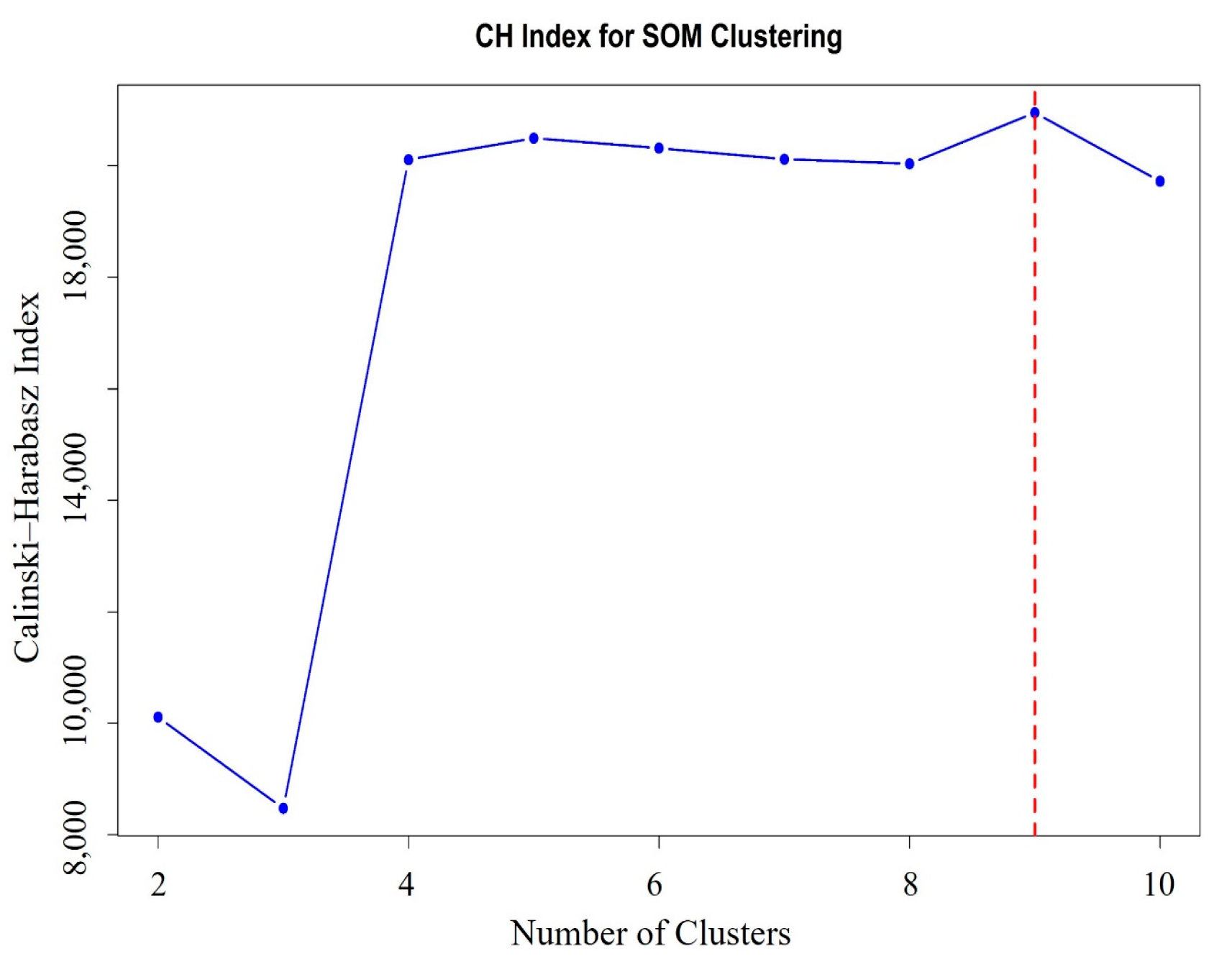
2.4. Identification of ES Supply–Demand Bundles

This study utilized the SOM algorithm to classify ES bundles at both the grid and city scales [47,48]. The SOM analysis was conducted using R version 4.3.2, primarily with the “kohonen” package (version 3.0.10). To further understand the interactions between supply and demand, the concepts of trade-offs and synergies were incorporated into the supply–demand bundle analysis to reveal interdependencies among different ecosystem services. The optimal number of bundles was determined using the Calinski–Harabasz Index (CH Index). The CH Index is a common clustering validity metric that evaluates cluster compactness and separation. A higher CH Index indicates better clustering quality, with greater inter-cluster separation and tighter intra-cluster cohesion. In this study, the CH Index reached its maximum when the number of ES bundles was set to nine, supporting the selection of nine bundle types as the basis for subsequent analysis (Figure 2). To validate the robustness of this result, a sensitivity analysis was conducted by adjusting SOM training parameters, including the number of iterations (rlen = 100 or 200), learning rate combinations (alpha start = 0.05 or 0.10; end = 0.01 or 0.05), and random seeds (123 and 2024). The CH Index was recalculated for each parameter set using the fpc package. The resulting CH values ranged from 20,687.88 to 21,513.06, with a mean of 21,270.65, a standard deviation of 259.45, and a coefficient of variation (CV) of 1.22%, reflecting a stable fluctuation range of 3.88%, thereby confirming the robustness of the nine-cluster solution.

The CH Index is defined as follows:

$$\mathrm{C}\mathrm{H}={\displaystyle \frac{\mathrm{t}\mathrm{r}(B_k)}{\mathrm{t}\mathrm{r}(W_k)}}\times {\displaystyle \frac{n-k}{k-1}}$$

(2)

where $\mathrm{t}\mathrm{r}(B_k)$ is the trace of the between-cluster dispersion matrix, $\mathrm{t}\mathrm{r}(W_k)$ is the trace of the within-cluster dispersion matrix, $n$ is the total number of observations, and $k$ is the number of clusters.

The specific characteristics of B1 to B9 are as follows (Figure 3): high-supply synergy bundles, exhibiting synergistic regions with high supply; moderate-supply synergy bundles, demonstrating synergistic relationships in supply, but generally lower than high-supply synergy bundles; low-supply trade-off bundles, characterized by trade-off relationships in supply; low supply–demand trade-off bundles, representing fewer supply and demand services, with trade-offs dominating the relationships between supply and demand services; high supply–demand trade-off bundles, characterized by a greater number of supply and demand services, with relationships consistent with B4; high-demand synergy bundles, where most demand services are high, exhibiting synergistic relationships; low supply–demand synergy bundles, where each service is scarce or nearly absent; and supply–demand scarcity bundles, characterized by the near absence of both supply and demand services.

2.5. Driver Analysis Based on Explainable Machine Learning Models

2.5.1. Model Selection and Evaluation

To select the most appropriate machine learning model for this study, a comparative analysis of five models—Random Forest (RF), Support Vector Machine (SVM), eXtreme Gradient Boosting (XGBoost), Light Gradient Boosting Machine (LightGBM), and Multiple Linear Regression (MLR)—was conducted. All input variables (X₁–X₁₅) were first standardized using z-score normalization to ensure consistency across varying data scales. The dataset was then randomly split into training (80%) and testing (20%) sets to evaluate model performance on unseen data. To avoid overfitting and ensure robustness, 5-fold cross-validation was applied, with average R² and RMSE used for supplementary evaluation. Model performance was assessed using both the coefficient of determination (R²) and the root mean square error (RMSE). While testing set performance was prioritized for selecting the final model, the cross-validation results provided additional evidence of generalizability. XGBoost outperformed all other models and was selected for SHAP-based driver analysis.

2.5.2. Variable Selection and SHAP-Based Driver Identification

To support the driver analysis, multi-source remote sensing data were integrated to ensure comprehensive factor selection. Specifically, the proportion of different land use types and land use intensity were calculated using ArcGIS 10.8, while landscape metrics were derived using FRAGSTATS 4.2. These indicators, along with other ecological, socioeconomic, and climate variables, were used to construct a candidate factor set. Subsequently, 18 potential drivers were identified from multiple dimensions, including ecological, socioeconomic, landscape, and natural climate factors. To address multicollinearity that could reduce interpretability, we performed VIF filtering using R 4.3.2 and the “car” package. Variables with a VIF value ≥ 10 were excluded, resulting in 15 representative and relatively independent factors (

Table 3. Drivers of ESDR selected in this study.

Category	Indicator	Code
Socioeconomic	GDP	X1
	POP	X2
	Land use degree	X3
Ecology	Normalized difference vegetation index	X4
	Net primary productivity	X5
	Forest cover ratio	X6
	Grassland cover ratio	X7
Natural climate	Land surface temperature	X8
	Precipitation	X9
	Digital elevation model	X10
	Slope	X11
Landscape	Aridity index	X12
	Connectivity index	X13
	Largest patch index	X14
	Landscape shape index	X15

). After preprocessing, SHAP was used with the XGBoost model to evaluate the influence and importance of each factor on ESDR [49,50,51].

3. Results

3.1. Spatiotemporal Dynamics of ES Supply and Demand

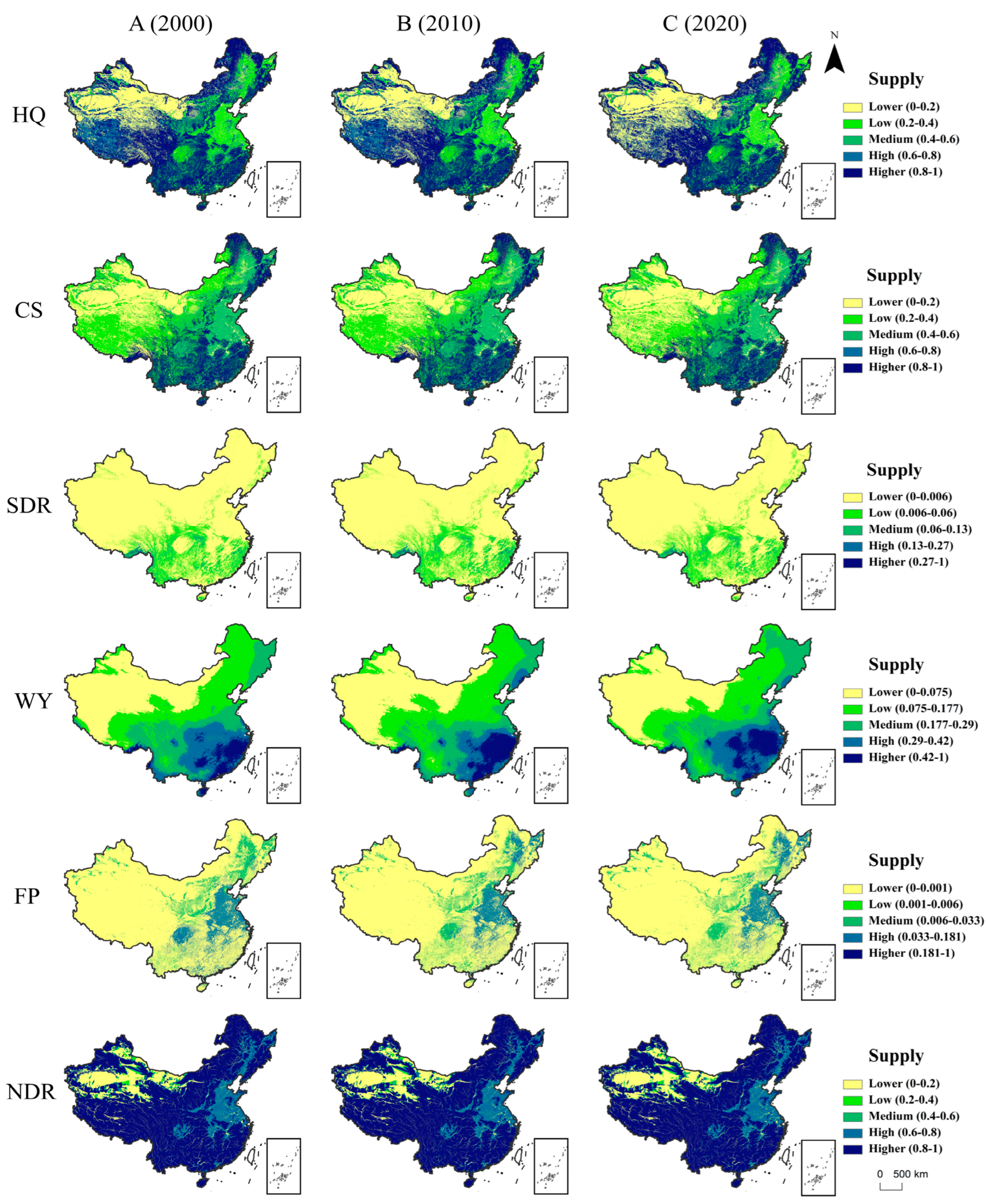
3.1.1. Analysis of ES Supply

ES supply in mainland China exhibits substantial spatial heterogeneity and overall temporal stability (Figure 4 and Figure S1). Over the past two decades, HQ and CS showed similar distribution patterns at both the grid and city scales, with high-value areas concentrated in southern mountainous regions and northeastern forests such as the Greater Khingan and Changbai Mountains. These areas coincide with biodiversity hotspots and ecologically protected zones, highlighting the role of natural reserves in supporting ecosystem functions. WY demonstrated a clear northwest-to-southeast gradient, reflecting variations in topography and precipitation and illustrating hydrological dependencies across different terrains. SDR was mainly distributed in the Hengduan Mountains, the Yunnan–Guizhou Plateau, and the Jiangnan Hills, corresponding to areas prone to soil erosion. The persistence of high SDR in erosion-prone zones indicates continued landscape vulnerability despite potential conservation efforts. FP showed high values across the three major plains, the Yellow River Basin, and the Sichuan Basin. Over time, its supply declined slightly in the Sichuan Basin but increased in the Northeast Plain, suggesting a spatial redistribution of agricultural productivity driven by changing land-use policies and resource availability. NDR maintained low values in the Taklamakan Desert, consistent with other ES types due to extreme arid conditions. At the city level, mean ES supply values generally increased, though trends varied by service and period. HQ and CS exhibited similar patterns across both scales. Average values of HQ, CS, SDR, and FP declined slightly, with SDR rising initially before declining. In contrast, WY and NDR showed upward trends, with WY increasing most notably, reflecting the combined effects of climate variability, upstream vegetation restoration, and water conservation projects.

3.1.2. Analysis of ES Demand

ES demand in mainland China exhibits significant spatial heterogeneity, with consistent distribution patterns across the grid and city scales (Figure 5 and Figure S2). Over the past two decades, CS, WY, and FP showed extensive low-value areas, whereas high-demand areas for these services were concentrated in the North China Plain and the middle and lower Yangtze River Plain. These densely populated and highly urbanized areas exhibited intensified demand pressures, underscoring the need for resource-efficient development. These regions, marked by high urbanization and population density, also experienced notable expansion of demand into adjacent zones. HQ and NDR displayed high demand levels in the eastern plains, southeastern hills, and the Sichuan Basin—areas known for intensive human–environment interactions. This spatial coupling between ecological sensitivity and human activity indicates potential ecological strain in socioeconomically active regions. In contrast, the northwestern desert regions remained consistently low in ES demand, indicating structural stability in areas with limited human activity. SDR had a relatively large proportion of low-value areas, but high-value regions expanded from the Hengduan Mountains toward the Qilian Mountains and the Yunnan-Guizhou Plateau. The expansion of SDR demand in erosion-prone zones may reflect increasing awareness or pressures related to land degradation control. At the city scale, the average ES demand values were higher than those at the grid scale. From 2000 to 2020, ES demand increased across all services, with WY, CS, and FP showing the largest gains. HQ and FP followed a pattern of initial decline followed by increase, while SDR and NDR experienced an early increase then subsequent decline. These dynamics suggest a growing urban–rural divergence, where socioeconomic transformations influence ecosystem service expectations.

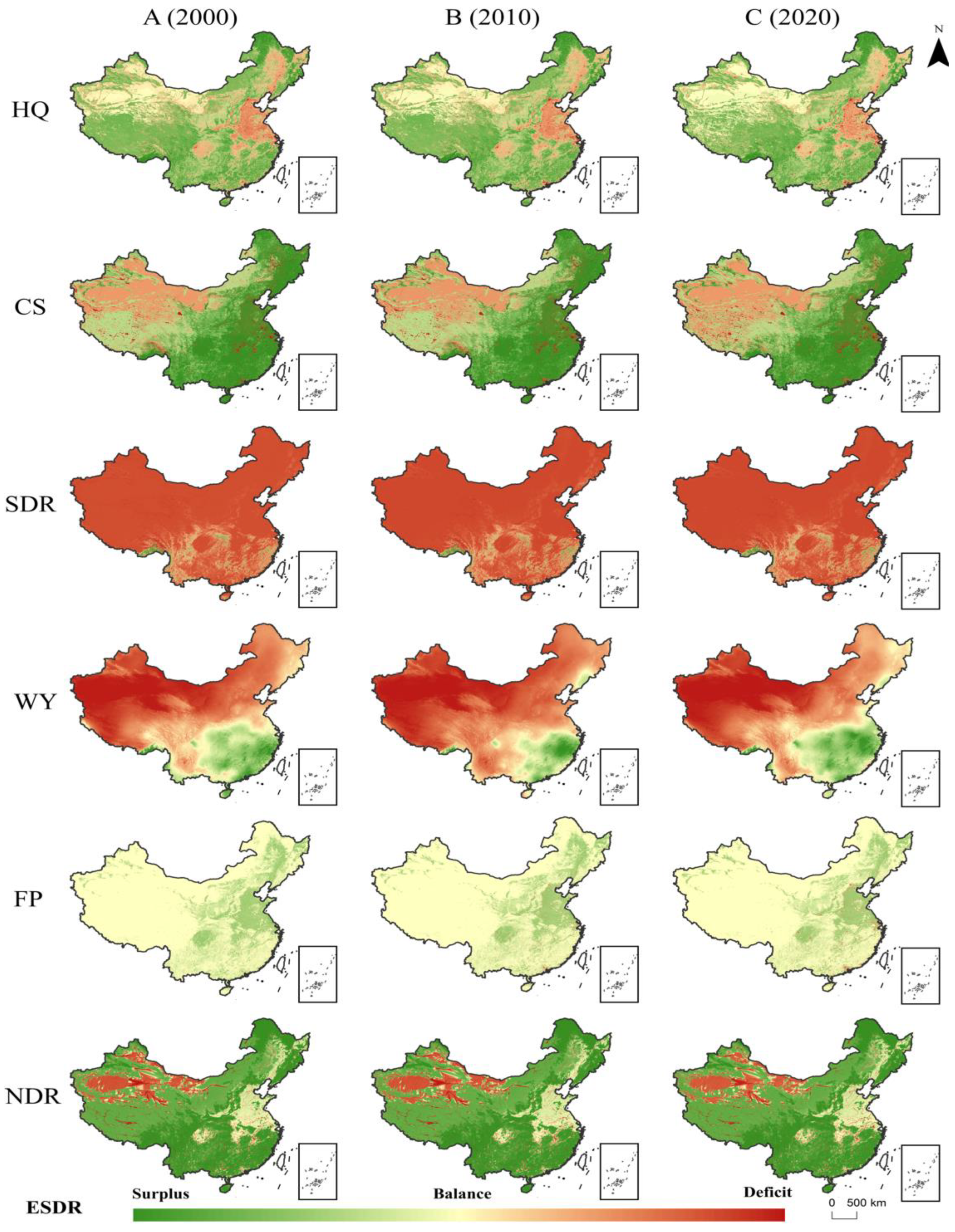
3.1.3. Analysis of ESDR

Spatial mismatches between ES supply and demand were widespread across mainland China (Figure 6 and Figure S3), with consistent large-scale patterns over time but increased detail at the grid scale. CS and NDR deficits were concentrated in the northwestern desert regions and gradually expanded toward the Kunlun and Gangdise Mountains. Surplus areas were mainly located in the northeastern mountains and the southern hilly regions. These polarizing mismatches suggest a growing divergence in resource allocation and ecological carrying capacity between underdeveloped and ecologically rich zones. Deficits in SDR and WY also persisted in the northwest and extended into the Inner Mongolian Plateau, indicating limited water retention and soil stability in these regions. In contrast, FP and HQ showed reversed patterns: HQ deficits overlapped with FP surpluses, particularly in the North China Plain, the Yangtze River Basin, and the Northeast Plain. These regions are characterized by intensive agriculture and urban development, where high food production coincides with lower habitat quality. Such contrasts exemplify a classic provisioning–regulating service trade-off, posing challenges for multifunctional land-use planning. Compared with other services, the supply–demand gaps of CS and NDR covered larger areas and exhibited clearer directional expansion. These patterns highlight the divergent spatial distribution of provisioning versus regulating services, shaped by both ecological constraints and land-use intensity. Recognizing these spatial tensions is essential for prioritizing ecological restoration and designing balanced land management policies.

3.2. Trade-Offs and Synergies in ES Supply and Demand

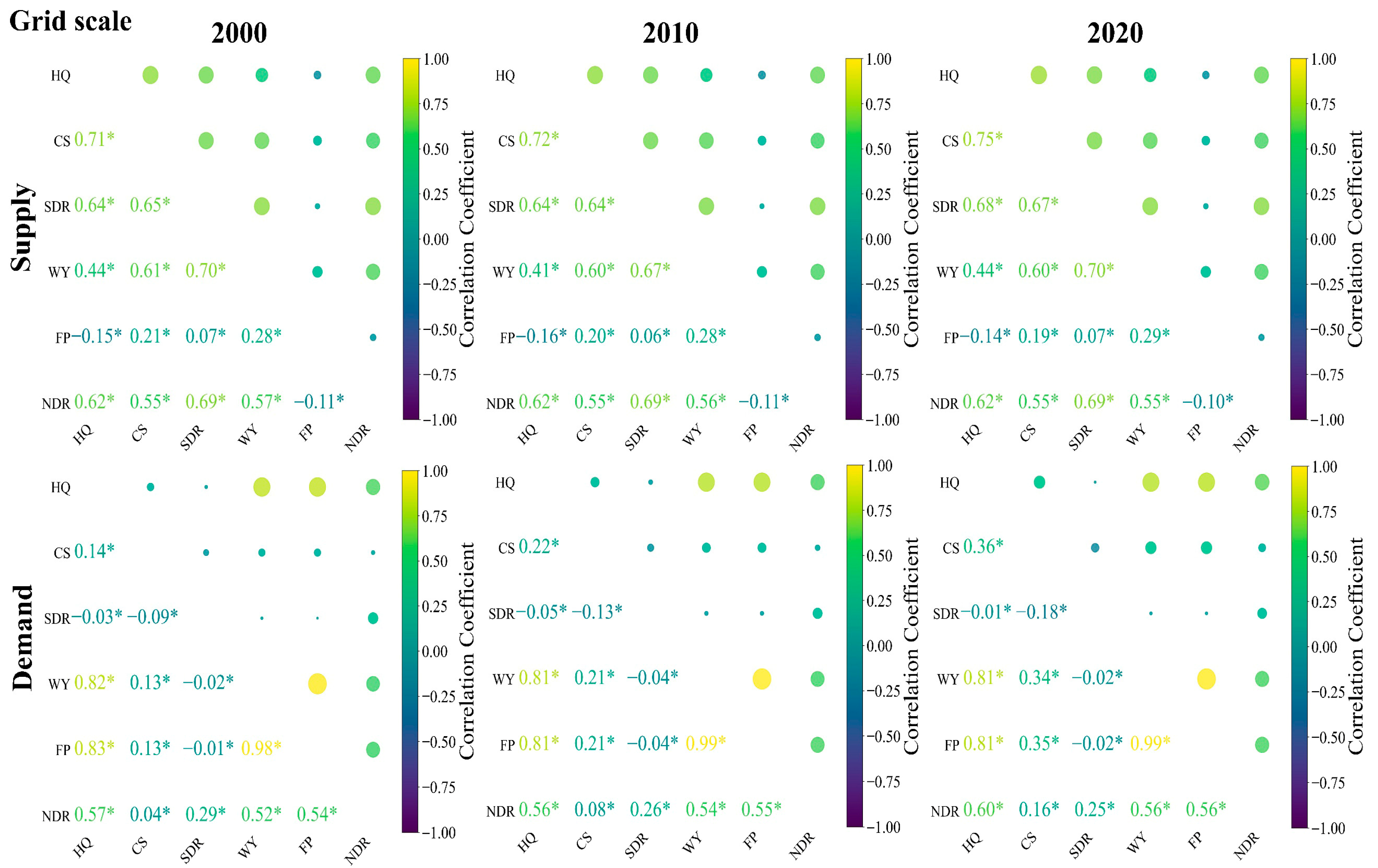
3.2.1. Spearman Correlation Analysis

All correlations between ES supply and demand were statistically significant (p < 0.05), confirming strong interdependencies among ecosystem functions (Figure 7). At the grid scale, the strongest synergy in supply was observed between CS and HQ, indicating concurrent benefits in ecologically intact areas. In contrast, the most pronounced trade-off occurred between FP and HQ, reflecting competing land-use priorities—namely, agricultural expansion versus biodiversity conservation. This pattern became more prominent at the city scale, suggesting that urban-driven land conversion has intensified conflicts between food production and ecological integrity. The synergy between NDR and HQ became more evident at broader scales, likely due to improved land management practices integrating nutrient retention with ecological protection. Temporal trends revealed scale-dependent shifts: at the grid scale, supply synergies strengthened while trade-offs declined from 2000 to 2020, likely due to local ecological restoration and vegetation recovery. By contrast, city-scale patterns showed weaker synergies and more pronounced trade-offs, possibly due to administrative boundaries aggregating diverse land uses and masking local ecological dynamics.

Demand-side correlations showed a similar trend. At the grid scale, synergies increased across 11 ES pairs, while at the city scale, synergistic interactions declined and trade-offs—particularly FP–HQ and FP–NDR—intensified. These spatial and temporal patterns point to growing sociopolitical pressures—such as urbanization, demographic expansion, and uneven resource allocation—that heighten competition for ecosystem benefits. Thus, the observed correlations are not merely statistical but are shaped by institutional and policy factors, including land-use planning, agricultural subsidies, and governance frameworks. Addressing ES conflicts effectively requires both ecological coordination and cross-scale institutional integration.

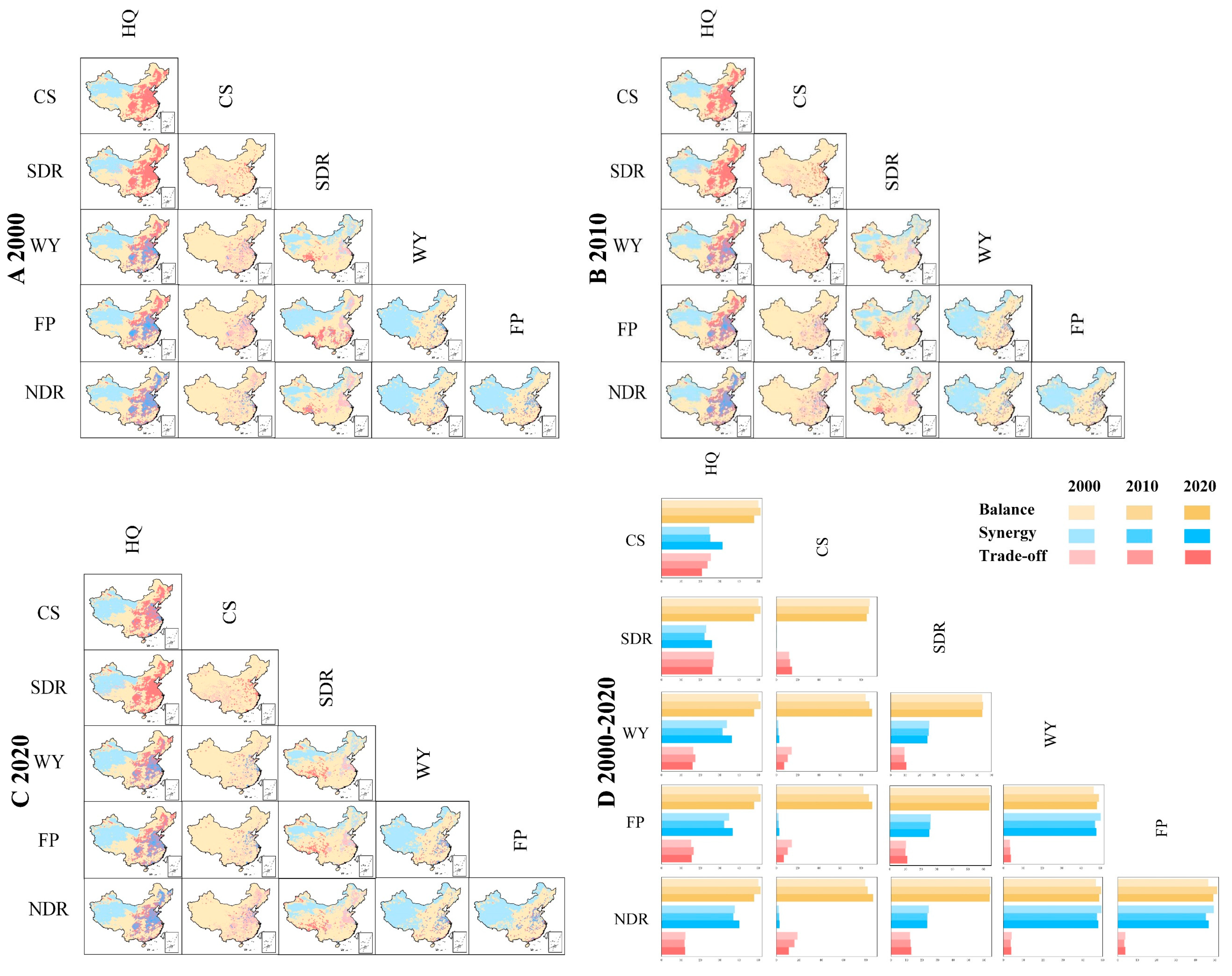
3.2.2. SpatioTemporal Patterns of Trade-Offs and Synergies

Spatial heterogeneity in ES supply–demand interactions was evident at both scales (Figure 8 and Figure S5). Over the past two decades, grid-scale supply synergies generally increased, except for six pairs—most involving NDR. Trade-offs weakened for most ES pairs, with exceptions such as WY–SDR and FP–CS, and combinations involving NDR. These results reflect evolving ecological relationships under environmental change and highlight persistent mismatches in NDR that may require targeted land-use adjustments or ecological compensation. At the city scale, the pattern reversed: most supply synergies declined while trade-offs intensified, especially for combinations involving FP and WY. However, synergies between CS–HQ and SDR–CS remained stable or improved, suggesting a partial alignment of carbon sequestration and soil retention with biodiversity conservation at broader scales. This indicates that multifunctional landscape planning still holds promise for maintaining ecosystem integrity in urbanizing regions, despite increasing service competition. Regarding demand, synergy among ES demands increased at the grid level, particularly for HQ and CS with other services (Figure 9 and Figure S6). Most demand-side trade-offs also weakened, except for a few involving SDR, FP, and NDR. These improvements suggest that coordinated management practices and local ecological programs have enhanced synergy at fine scales. In contrast, city-scale synergies declined and trade-offs became more pronounced, especially in combinations involving FP and NDR, indicating increasing urban demand pressure and spatial competition among services. This underscores the need for balancing urban expansion with ecological resilience in high-demand regions.

Spatially, synergy in ES supply dominated over trade-offs for most pairs, particularly in northwest deserts and southern mountain regions. NDR–FP was an exception, with nearly equal proportions of synergy and trade-off in southeastern hills and northeastern plains. For demand, synergy also prevailed, especially in the Qinghai–Tibet Plateau and northwest plateaus. Trade-offs were more localized, with CS–HQ and SDR–HQ trade-offs concentrated in the North China Plain, northeast, and Sichuan Basin. Other pairs, such as WY–SDR and FP–SDR, clustered in the Hengduan Mountains and Yunnan–Guizhou Plateau. Overall, spatial interactions—both synergistic and competitive—were more distinct at the grid scale, while city-level patterns were comparatively muted. This underscores the finer sensitivity of grid-based analyses in capturing ES dynamics and spatial tensions, reinforcing their value for detecting early ecological warning signals and informing spatial policy.

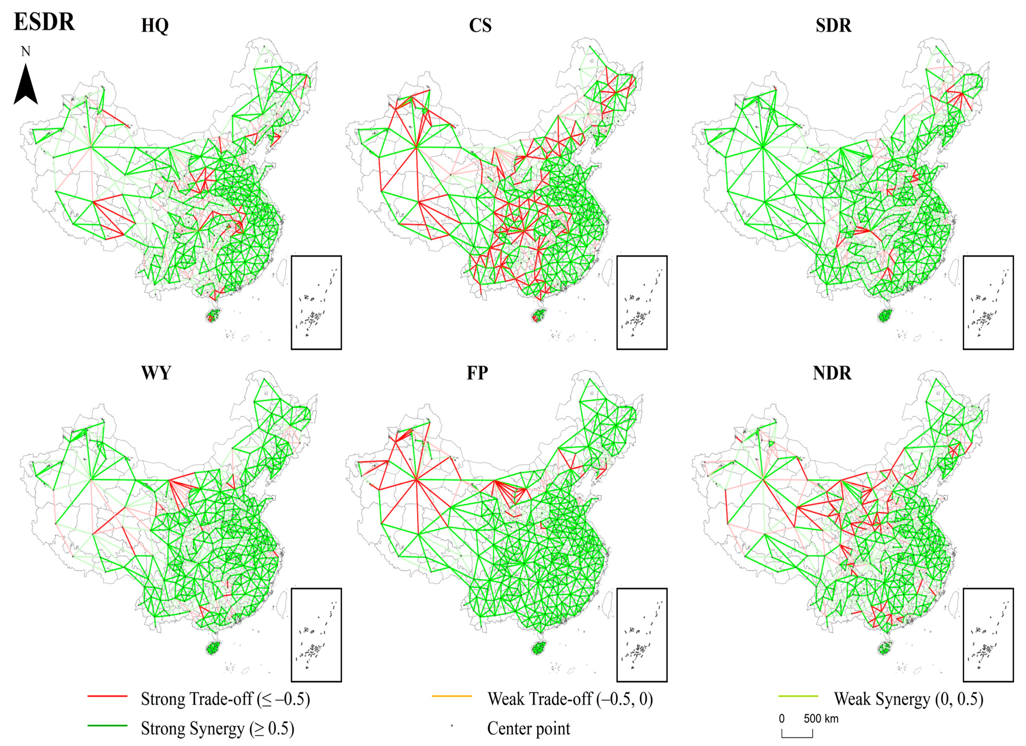
3.2.3. Interactive Spatio-Temporal Visualization of Trade-Offs and Synergies

Through further investigation of the spatiotemporal trade-offs and synergies in the supply–demand ratio, it was found that the trade-off ratio for SDR and WY in adjacent municipal areas was relatively low. SDR was primarily concentrated in the northeastern and central–southern regions of the study area, while WY was mainly located in the northwestern region (Figure 10). This spatial separation reflects contrasting biophysical conditions and land-use patterns. The trade-off ratio of HQ was higher, primarily distributed in areas such as Ulanqab, Yan’an, Huanggang, Nagqu, and Maoming. FP displayed pronounced spatial heterogeneity, with trade-offs concentrated in northern and northwestern areas where urban expansion and land conversion pressures are high. CS and NDR exhibited the highest trade-off ratios, accounting for 25.4% and 18.6%, respectively. Various ES results indicated that persistent trade-off signals were concentrated in central–western China and parts of northeastern China. This spatial clustering reflects long-term mismatches between supply and demand, highlighting priority areas for targeted ecological management.

3.3. Spatial Differentiation of ES Supply–Demand Bundles Across Dual Scales

The results demonstrate distinct spatial distributions of ES supply–demand bundles at the grid and city scales (Figure 11). At the grid scale, B3 occupies the largest proportion (29.1%), concentrated in the Tianshan Mountains, Qinghai–Tibet Plateau, Inner Mongolia Plateau, and Greater Khingan Range. Supply-dominated bundles B1 and B2 are distributed in southern mountainous areas, the Changbai Mountains, and the Hengduan–Yunnan–Guizhou region. Demand-dominated bundle B7 has the lowest proportion and is sparsely distributed in densely populated areas, such as the upper Yellow River and Yangtze River Delta. At the city scale, B8 accounts for the largest proportion (26.5%), mainly located in the Taklamakan Desert, Loess Plateau, and Greater Khingan Range. Supply-dominated bundles B2, B3, and B6 are, respectively, located in the southern mountain regions, western Qinghai–Tibet Plateau, and areas such as the Qaidam Basin and Qinling Mountains. Some bundles, such as B3 and B2, exhibit similar spatial patterns across scales, while others appear only at one scale. These differences underscore the need for scale-specific ES management strategies, as grid-level bundles are shaped more by biophysical factors (e.g., elevation, vegetation), whereas city-level patterns reflect administrative and socioeconomic structures, contributing to divergent supply–demand imbalances.

3.4. Dual-Scale Driver Analysis

3.4.1. Model Performance Evaluation

We constructed five predictive models to assess their performance across two scales (

Table 4. Performance comparison among machine learning models.

Model	Grid Scale		City Scale
	R2	RMSE	R2	RMSE
SVM	0.742	0.169	0.882	0.104
RF	0.79	0.084	0.93	0.02
XGBoost	0.798	0.081	0.939	0.017
LightGBM	0.796	0.083	0.936	0.018
MLR	0.782	0.14	0.922	0.076

). To ensure consistency and robustness, all models were trained on 80% of the dataset and validated on the remaining 20%. We also applied 5-fold cross-validation to evaluate each model’s generalization ability. The results indicate that while LightGBM performed comparably to XGBoost at both scales, the latter showed superior performance, with the highest R² (0.798 at the grid scale, 0.939 at the city scale) and the lowest RMSE (0.081 and 0.017, respectively). In cross-validation, XGBoost also demonstrated the best generalization capability, maintaining the highest average R² (0.7367) and the lowest RMSE (0.1726), followed by Random Forest and LightGBM. By contrast, SVM and MLR performed less consistently (R² = 0.6984 and 0.6292; RMSE = 0.1847 and 0.2048, respectively). These results confirm that XGBoost offered both high accuracy and stability, supporting its selection as the optimal model for subsequent SHAP-based driver mechanism analysis.

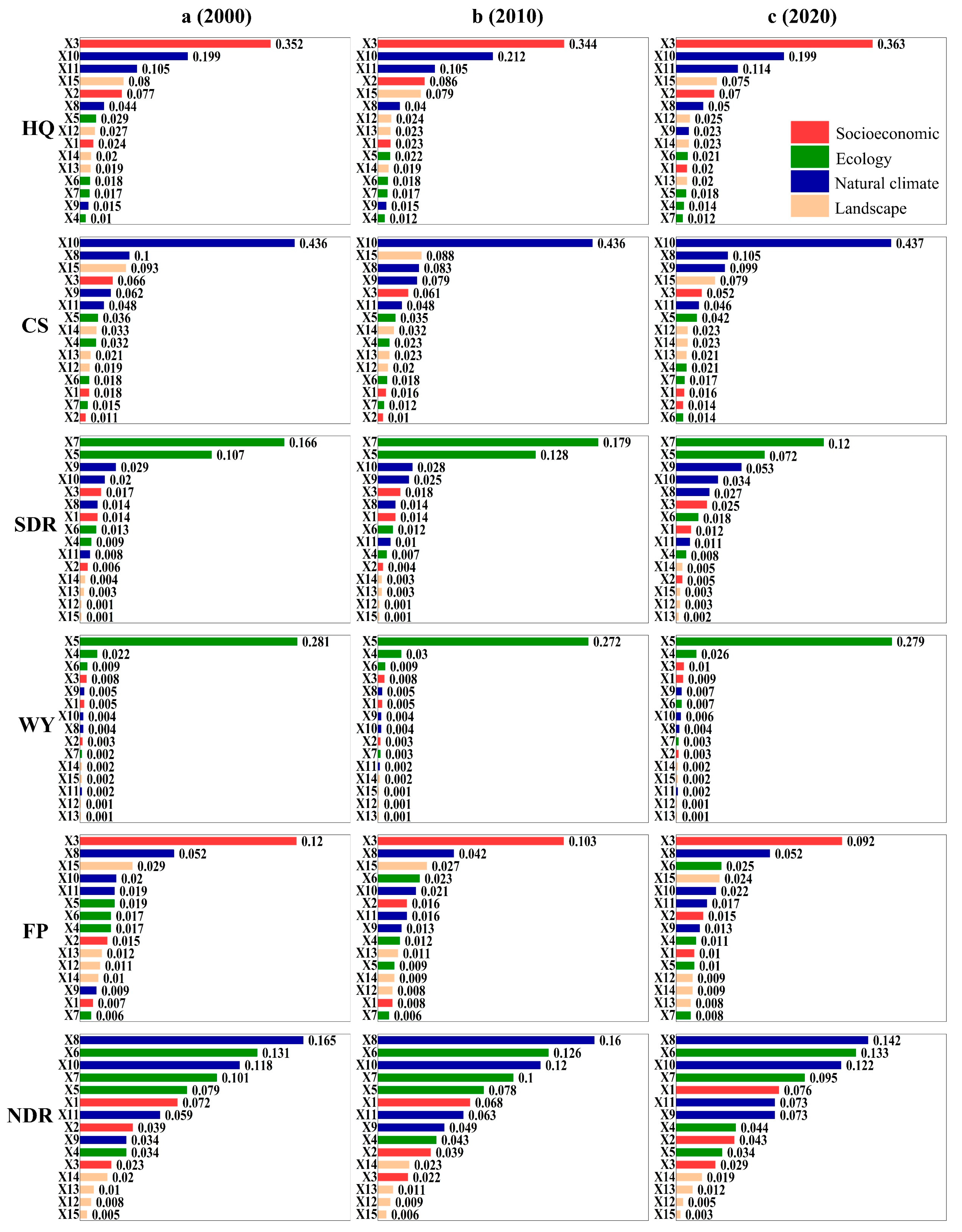
3.4.2. Analysis of Driving Factors at the Grid Scale

The results indicate the following: (1) HQ, SDR, and NDR remained consistently dominated by the same key factors throughout the study period. HQ was primarily influenced by socioeconomic and natural climate factors, with increasing SHAP values for socioeconomic factor X3. SDR was shaped by ecological and climate variables, while NDR was influenced by natural climate and ecological factors. For both SDR and NDR, higher values of key ecological and climate variables contributed positively to ES supply. (2) The dominant drivers of CS shifted over time. Initially, CS was influenced by natural climate and landscape factors, with low values of landscape factor X15 negatively associated with it. In later years, CS became predominantly driven by natural climate factors, and higher feature values consistently had positive effects; (3) WY was initially driven by ecological factors, but socioeconomic factor X3 replaced ecological factor X6 in the later stages. Notably, low values of X4 contributed positively to WY, suggesting nonlinear threshold effects; (4) FP exhibited a transition from socioeconomic, climate, and landscape drivers to ecological dominance over time. The influence of socioeconomic factor X3 declined, while natural climate factor X8 remained positively associated with FP. These shifts reflect FP’s increasing ecological sensitivity under long-term land use dynamics.

3.4.3. Analysis of Driving Factors at the City Scale

The results show the following: (1) HQ was consistently influenced by socioeconomic, natural climate, and ecological factors. SHAP values for socioeconomic factor X3 increased over time, with lower feature values having a positive effect. (2) CS was mainly driven by natural climate and socioeconomic factors, particularly X8 and X10. Over time, the contribution of socioeconomic factor X3 declined, indicating a shift toward climate-dominated control. (3) SDR maintained stable ecological and climate drivers, with high feature values consistently associated with higher SDR levels. (4) FP was influenced by both socioeconomic and ecological factors. Ecological factor X7 showed an inverse relationship with FP—lower values of X7 corresponded to higher FP supply. (5) NDR experienced a shift in dominant drivers. Initially influenced by natural climate and socioeconomic factors (X10, X11, and X3), the importance of ecological factor X6 increased significantly over time. By the end of the study period, X6 surpassed X3 in importance, and higher values of X6 positively contributed to NDR. This change reflects the growing influence of ecological conditions in regulating NDR at broader spatial scales.

4. Discussion

4.1. The Characteristics of ES Supply and Demand

Investigating ES from the perspective of supply and demand plays a key role in supporting sustainable development [52]. The evaluation of supply–demand relationships is shaped by scale effects, as different scales of analysis can lead to varied outcomes [53]. To verify differences across spatial patterns at multiple scales, we examined both a 1 km grid and the city level to enhance result precision. Our analysis highlighted notable spatial variation in ES supply and demand at these scales. For supply services, built-up land identified at the grid level often corresponded to low-value areas. As the scale increased, however, the mix of land-use types tended to balance out, converting some low-value areas into higher-value zones [54,55,56]. In demand services, high-value areas for HQ demand in the Sichuan Basin and Northeast Plain showed a decreasing trend with an increasing scale (Figure 5 and Figure S2), a pattern confirmed in this study.

Overall, supply services demonstrated a decreasing trend from southeast to northwest (Figure 4 and Figure S1). The spatial distributions of HQ and NDR were similar, with high-value areas concentrated in the Greater Khingan Mountains, Qinghai–Tibet Plateau, Hengduan Mountains, and southern mountainous and hilly regions. These areas, characterized by continuous forest landscapes, provide biodiversity habitats and possess strong water regulation capacity. High-value zones for CS and WY were concentrated in the southern mountainous areas and the Changbai Mountains in the northeast. These regions supply abundant water and feature superior vegetation cover, enhancing CS and WY supply capacity. High-value zones for SDR and FP were located in the southern and eastern parts of the study area, respectively. SDR benefited from humid subtropical and tropical climates that promoted vegetation growth and improved soil retention, while extensive cultivated land and agricultural modernization in the east enhanced FP. In terms of demand, high-value zones for CS, WY, and FP were largely distributed in the Beijing–Tianjin–Hebei urban agglomeration, the North China Plain, and the Yangtze River Delta. High population density and urbanization in these regions drove significant demand for FP, CS, and WY (Figure 5 and Figure S2). Likewise, HQ and SDR demand peaked in central–eastern and southern regions, where agriculture and industry intensified pressure on HQ and NDR. The supply–demand ratio revealed consistent imbalance zones for HQ, CS, WY, and NDR. CS and WY imbalance areas expanded from the northwestern deserts to eastern and southern regions (Figure 6 and Figure S3), indicating the limits imposed by arid climates and sparse vegetation. SDR imbalances were concentrated in central and northern areas, while the Lancang River and lower Yangtze River Plain remained relatively unaffected. FP surplus zones were clustered in the North China Plain, Northeast Plain, and Sichuan Basin, and their extent increased over time.

A comprehensive examination of spatiotemporal dynamics in ES supply and demand is essential for regional management [6]. The findings revealed significant trade-offs between FP, NDR, and other services at both scales, with most trade-offs concentrated in the southern hilly regions, Greater Khingan Mountains, and North China Plain (Figure 7, Figure 8, Figure 9 and Figures S4–S6). Trade-offs between SDR demand and other demand services were especially pronounced in the central plains and southern Hengduan Mountains, while other demand services showed more synergistic relationships. This suggests a close link between ES demand distribution and factors such as human activity and land-use patterns. Comparisons of supply–demand trade-offs and synergies across scales showed that the grid scale better captured spatial aggregation and temporal dynamics, outperforming the city scale in identifying interaction patterns. Spatiotemporal interaction network analysis of the supply–demand ratio also revealed strong spatial differentiation in ESDR across mainland China (Figure 10), with western and northern regions generally following a trade-off pattern, especially involving HQ, CS, and NDR. These results highlight imbalances in development and resource allocation in these areas.

The observed mismatches and evolving trade-offs suggest that grid-scale analysis can more effectively uncover micro-regional disparities in ES demand, often shaped by complex sociopolitical contexts such as zoning, infrastructure, and land access policies. Synergies in HQ and CS demand at finer resolutions indicate the potential for place-based ecological planning, where investments in green infrastructure and localized conservation can be aligned with emerging needs. In contrast, intensified trade-offs at coarser scales reflect structural tensions in regional development strategies, emphasizing the need for integrated planning that reconciles economic growth with ecological sustainability.

To further understand spatial mismatches, scale effects, and dynamic ES interactions, we compared our findings with previous studies. Earlier research [56] generally suggested that increasing the spatial scale intensifies trade-offs due to greater land-use overlap and heterogeneity. However, other studies [27] argued that supply–demand imbalances may be alleviated at broader scales, as ecological deficit areas are smoothed out through spatial aggregation. Our findings integrate both perspectives to some extent. Trade-offs between services such as CS and HQ do become more pronounced at larger scales, especially in underdeveloped western regions. Conversely, synergistic relationships become clearer in highly urbanized areas. Some mismatch patterns are attenuated at coarser spatial resolutions. These variations may reflect differences in landscape fragmentation, the directionality of service flows, or dominant regional drivers. Therefore, our findings emphasize the importance of incorporating both scale sensitivity and service-specific characteristics when analyzing ES dynamics, especially in the context of multi-scale spatial planning and regional ecological governance.

4.2. Influence of Spatial Scale on Driving Factors

Understanding the drivers behind ES trade-offs requires analyzing both the direction and strength of influence on the supply–demand ratio (ESDR) [57,58]. Our results show that these drivers vary by scale. At the grid level, HQ, FP, and WY are shaped largely by socioeconomic factors. At the city level, these factors dominate nearly all services except SDR (Figure 12 and Figure S7), indicating that spatial scale affects the balance between human and ecological influences—finer resolutions capture localized pressures and environmental responses suitable for precision interventions, while city-scale patterns reflect broader governance priorities and cross-jurisdictional coordination needs.

To contextualize our findings, we compared them with studies using similar methods. One such study found that land use, GDP, and NDVI had greater explanatory power at the watershed level than at the 1 km grid scale [59]. While both studies employed high-resolution data, that research focused on interactions among service supplies, whereas ours focused on the supply–demand ratio (ESDR). We found socioeconomic drivers to be more influential at the city scale. This difference likely stems from varying spatial units and research perspectives. The watershed-based study examined ecological covariation within natural boundaries, whereas our ESDR-based approach emphasizes demand, making socioeconomic variables more prominent, particularly in urban areas where such factors are spatially concentrated. Accordingly, urban-level ES management should integrate land-use policy with socioeconomic development planning, especially in rapidly urbanizing regions. For example, zoning adjustments and targeted ecological compensation mechanisms could help mitigate demand-driven ecological stress.

Driver stability also differed by scale [60,61]. At the grid level, dominant factors remained relatively stable over time, reflecting persistent local patterns. At the city scale, drivers shifted more markedly in response to regional policy, planning, or economic change (Figure 13 and Figure S8). This temporal variability at broader scales supports the need for adaptive governance frameworks capable of responding to evolving development trajectories and shifting policy contexts. In contrast, grid-scale stability underscores the importance of long-term ecosystem monitoring and locally grounded conservation efforts. While the dominant drivers of ESDR varied across services and scales—spanning ecological, climatic, and socioeconomic dimensions—governance and institutional capacity, though not explicitly modeled, may play a decisive yet underappreciated role. The divergent ESDR outcomes observed in regions with comparable socioecological characteristics reinforce this point. For example, stricter enforcement of land-use regulation or more robust compensation schemes often corresponded to improved supply–demand alignment. These findings underscore the need to move beyond static biophysical explanations and incorporate institutional and policy factors into ES analysis. Future studies could incorporate governance indicators—such as ecological investment per capita, policy intensity indices, or enforcement metrics—to capture the institutional dimension of ES mismatches more fully. Overall, these results highlight the importance of scale-aware and service-specific approaches when evaluating ES dynamics. Without this nuance, spatial planning and governance efforts may overlook key regional drivers.

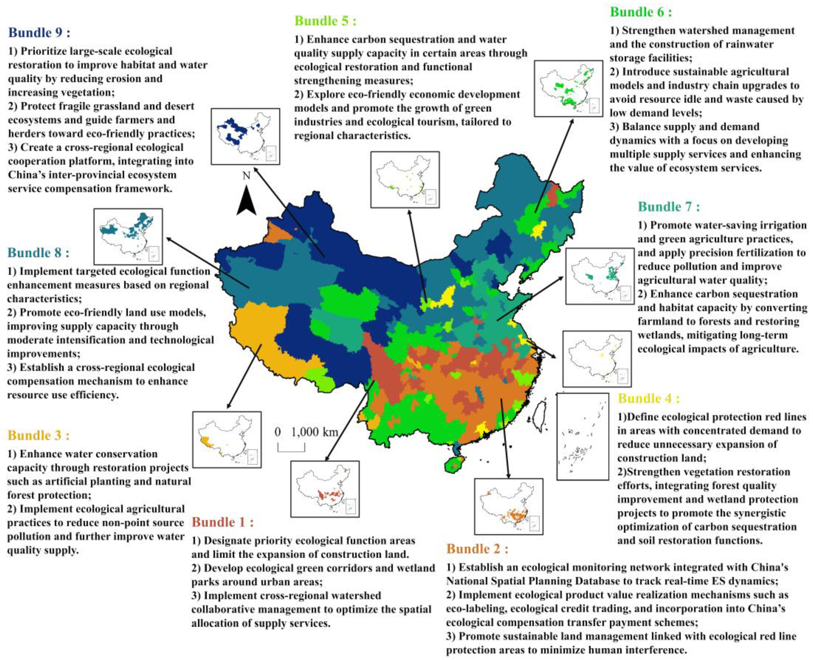
4.3. Localized Management Strategies for Dual-Scale ES Supply–Demand Bundles

To effectively implement the results of ES bundle identification, we developed spatially differentiated strategies at both grid and city scales (Figure 14 and Figure 15). These strategies respond to trade-offs and synergies within bundles, account for dominant influencing factors, and incorporate China’s existing ecological governance tools such as National Land Spatial Planning (2021–2035), the Ecological Red Line policy, and regional ecological compensation mechanisms [62]. Tailored responses from different spatial perspectives are essential for achieving long-term sustainability goals [63]. At the city scale, Bundle 7—located primarily in the North China Plain and lower Yangtze River Basin—represents high-provisioning but trade-off-intensive regions. For these areas, returning farmland to forests and wetlands is critical to enhancing CS and HQ services, aligning with the Grain for Green Program, and reinforcing ecological red line enforcement to ensure controlled urban expansion and sustainable agricultural transitions. Precision agriculture and green infrastructure should be promoted to mitigate non-point source pollution and improve multifunctional land use. Bundle 9, concentrated in Northwest China, covers ecologically degraded zones with extreme climate exposure, where large-scale ecological restoration projects should align with China’s Major Function-Oriented Zoning and the Three-North Shelterbelt Program. Inter-provincial ecological compensation platforms and real-time monitoring stations are also recommended to improve ecosystem service flows and strengthen regional resilience. Bundle 2, distributed in the southern hilly zones, reflects synergy bundles with high HQ and water regulation services. Ecological monitoring systems should be integrated with the National Spatial Planning Database, while biodiversity corridors can be protected and eco-tourism promoted through mechanisms like the Ecological Product Value Realization Mechanism. At the grid scale, strategies prioritize precision and site-specific ecological needs. For instance, Bundle 1—commonly located along river valleys—should focus on delineating micro-scale ecological corridor protection zones under the Ecological Red Line framework, supported by village-level forest restoration pilots and participatory conservation programs. Bundle 6, found in mountainous farming areas, should prioritize the construction of micro-reservoirs and rainwater harvesting systems, integrated into county-level water management and linked with national subsidies. Grid-level Bundle 9, covering desert-prone zones, requires localized drought-adaptive strategies, including the introduction of stress-tolerant crops, sustainable land management training, and early warning systems—all aligned with the National Desertification Control Plan and ecological compensation pilots. By embedding these bundle-based recommendations within China’s existing institutional frameworks, this approach enhances the policy relevance and actionable integration of ES assessments for sustainable land use governance.

5. Conclusions

This study systematically investigated the multi-scale spatiotemporal dynamics, trade-offs, synergies, and driving mechanisms of ES supply–demand relationships across mainland China to support regional sustainable development. By integrating spatiotemporal analysis, SOM, and interpretable machine learning models, we revealed significant heterogeneity in ES supply, demand, and supply–demand ratios, with higher supply values concentrated in the east and south and demand hotspots in densely populated central and eastern regions. The analysis at the grid scale proved more effective in detecting spatial clustering patterns, while trade-offs and synergies exhibited differences across scales. The spatiotemporal interaction network highlighted regional imbalances, with pronounced supply–demand mismatches in the western and northern regions. Nine distinct supply–demand bundles were identified, offering a scientific basis for differentiated and scale-specific ecosystem management strategies. Using XGBoost combined with SHAP interpretability, we identified key drivers of supply–demand dynamics, demonstrating the scale-dependent roles of ecological, climatic, and socioeconomic factors; in particular, socioeconomic drivers exerted a stronger influence at the city scale. Overall, this study enhances our understanding of ES supply–demand dynamics and provides practical insights for ecosystem governance and sustainable policy-making in China. Based on the identified spatial mismatches and driving mechanisms, several policy recommendations are proposed: (1) In ecologically underperforming areas such as the Sanjiangyuan region and the Inner Mongolia Plateau, efforts should focus on constructing ecological corridors and restoring habitats. These measures should be integrated with regional development priorities to enhance ecosystem service connectivity and spatial flow. (2) In central agricultural regions such as the North China Plain and Northeast Plain, integrated strategies combining farmland conservation, water resource management, and green infrastructure can enhance regulating services (e.g., HQ, CS) while ensuring food security. (3) In the ecologically fragile areas along the desert margins of northwest China, efforts should focus on building ecological buffer zones and managing water resources, in conjunction with anti-desertification and oasis restoration programs, to strengthen basic supply capacity and regional resilience.

This study has several limitations. First, the exclusion of cultural and some supporting services (e.g., pollination, aesthetic value) may compromise assessment completeness. These services are vital to human well-being but are difficult to quantify due to the lack of standardized indicators and large-scale spatial data, particularly in culturally diverse or densely populated areas. Second, while the dual-scale framework enhances spatial analysis, cross-scale feedback remains underexplored. Understanding how local land-use changes influence city-level patterns, or how macro policies affect micro-level decisions, requires future research using nested modeling and scale-linkage approaches. Third, the analysis used only three time points, limiting the ability to capture dynamic shifts from climate extremes or policy changes. Future studies should incorporate scenario-based simulations, remote sensing time series, and social perception data to better reflect the non-stationary nature of ES dynamics. Overall, advancing service inclusion, scale integration, and temporal modeling will improve support for ecosystem governance and planning.

References

1. Gallardo, B.; Bacher, S.; Barbosa, A.M.; Gallien, L.; González-Moreno, P.; Martínez-Bolea, V.; Sorte, C.; Vimercati, G.; Vilà, M. Risks posed by invasive species to the provision of ecosystem services in Europe. Nat. Commun. 2024, 15, 2631. [Google Scholar] [CrossRef]
2. He, L.; Xie, Z.; Wu, H.; Liu, Z.; Zheng, B.; Wan, W. Exploring the interrelations and driving factors among typical ecosystem services in the Yangtze river economic Belt, China. J. Environ. Manag. 2024, 351, 119794. [Google Scholar] [CrossRef] [PubMed]
3. Liu, C.; Yang, M.; Hou, Y.; Xue, X. Ecosystem service multifunctionality assessment and coupling coordination analysis with land use and land cover change in China’s coastal zones. Sci. Total Environ. 2021, 797, 149033. [Google Scholar] [CrossRef]
4. Xu, W.; Xiao, Y.; Zhang, J.; Yang, W.; Zhang, L.; Hull, V.; Wang, Z.; Zheng, H.; Liu, J.; Polasky, S.; et al. Strengthening protected areas for biodiversity and ecosystem services in China. Proc. Natl. Acad. Sci. USA 2017, 114, 1601–1606. [Google Scholar] [CrossRef] [PubMed]
5. Cui, F.; Tang, H.; Zhang, Q.; Wang, B.; Dai, L. Integrating ecosystem services supply and demand into optimized management at different scales: A case study in Hulunbuir, China. Ecosyst. Serv. 2019, 39, 100984. [Google Scholar] [CrossRef]
6. Yuan, Y.; Bai, Z.; Zhang, J.; Huang, Y. Investigating the trade-offs between the supply and demand for ecosystem services for regional spatial management. J. Environ. Manag. 2023, 325, 116591. [Google Scholar] [CrossRef]
7. Xue, C.; Xue, L.; Chen, J.; Tarolli, P.; Chen, X.; Zhang, H.; Qian, J.; Zhou, Y.; Liu, X. Understanding driving mechanisms behind the supply-demand pattern of ecosystem services for land-use administration: Insights from a spatially explicit analysis. J. Clean. Prod. 2023, 427, 139239. [Google Scholar] [CrossRef]
8. Gou, M.; Li, L.; Ouyang, S.; Wang, N.; La, L.; Liu, C.; Xiao, W. Identifying and analyzing ecosystem service bundles and their socioecological drivers in the Three Gorges Reservoir Area. J. Clean. Prod. 2021, 307, 127208. [Google Scholar] [CrossRef]
9. Tian, P.; Liu, Y.; Li, J.; Pu, R.; Cao, L.; Zhang, H. Spatiotemporal patterns of urban expansion and trade-offs and synergies among ecosystem services in urban agglomerations of China. Ecol. Indic. 2023, 148, 110057. [Google Scholar] [CrossRef]
10. Feng, Z.; Jin, X.; Chen, T.; Wu, J. Understanding trade-offs and synergies of ecosystem services to support the decision-making in the Beijing–Tianjin–Hebei region. Land. Use Policy 2021, 106, 105446. [Google Scholar] [CrossRef]
11. Huang, J.; Xia, Z.; Liu, L. Impacts of landscape configurations on ecosystem services and their trade-offs across different landscape compositions. Ecosyst. Serv. 2024, 70, 101666. [Google Scholar] [CrossRef]
12. Zuo, L.; Gao, J. Investigating the compounding effects of environmental factors on ecosystem services relationships for Ecological Conservation Red Line areas. Land. Degrad. Dev. 2021, 32, 4609–4623. [Google Scholar] [CrossRef]
13. He, G.; Zhang, L.; Wei, X.; Jin, G. Scale effects on the supply–demand mismatches of ecosystem services in Hubei Province, China. Ecol. Indic. 2023, 153, 110461. [Google Scholar] [CrossRef]
14. Ou, D.H.; Wu, N.J.; Li, Y.X.; Ma, Q.; Zheng, S.Y.; Li, S.Q.; Yu, D.R.; Tang, H.L.; Gao, X.S. Delimiting Ecological Space and Simulating Spatial-Temporal Changes in Its Ecosystem Service Functions Based on a Dynamic Perspective: A Case Study on Qionglai City of Sichuan Province, China. J. Resour. Ecol. 2022, 13, 1128–1142. [Google Scholar] [CrossRef]
15. Chang, B.; Chen, B.; Chen, W.; Xu, S.; He, X.; Yao, J.; Huang, Y. Analysis of trade-off and synergy of ecosystem services and driving forces in urban agglomerations in Northern China. Ecol. Indic. 2024, 165, 112210. [Google Scholar] [CrossRef]
16. Jin, G.; Deng, X.Z.; Dong, Y.; Wu, F. China’s multidimensional poverty measurement and its spatiotemporal interaction characteristics in the perspective of development geography. Acta Geogr. Sin. 2020, 75, 1633–1646. [Google Scholar]
17. Geng, Y.W.; Li, X.S.; Chen, J.Q.; Liu, X.Z.; Zhang, J.X.; Cheng, J.M. Coupling relationship and transition mechanism between resilience and efficiency in China’s territorial space. Acta Ecol. Sin. 2024, 44, 6003–6019. [Google Scholar]
18. Liu, J.; Wang, H.; Hui, L.; Tang, B.; Zhang, L.; Jiao, L. Identifying the Coupling Coordination Relationship between Urbanization and Ecosystem Services Supply–Demand and Its Driving Forces: Case Study in Shaanxi Province, China. Remote Sens. 2024, 16, 2383. [Google Scholar] [CrossRef]
19. Xu, J.; Wang, S.; Xiao, Y.; Xie, G.; Wang, Y.; Zhang, C.; Li, P.; Lei, G. Mapping the spatiotemporal heterogeneity of ecosystem service relationships and bundles in Ningxia, China. J. Clean. Prod. 2021, 294, 126216. [Google Scholar] [CrossRef]
20. Yuan, Z.; Liang, Y.; Zhao, H.; Wei, D.; Wang, X. Trade-offs and synergies between ecosystem services on the Tibetan Plateau. Ecol. Indic. 2024, 158, 111384. [Google Scholar] [CrossRef]
21. Sun, X.; Liu, H.; Liao, C.; Nong, H.; Yang, P. Understanding recreational ecosystem service supply-demand mismatch and social groups’ preferences: Implications for urban-rural planning. Landsc. Urban. Plan. 2024, 241, 104903. [Google Scholar] [CrossRef]
22. Zhou, B.; Chen, G.; Yu, H.; Zhao, J.; Yin, Y. Revealing the Nonlinear Impact of Human Activities and Climate Change on Ecosystem Services in the Karst Region of Southeastern Yunnan Using the XGBoost–SHAP Model. Forests 2024, 15, 1420. [Google Scholar] [CrossRef]
23. Ouyang, N.; Rui, X.; Zhang, X.; Tang, H.; Xie, Y. Spatiotemporal evolution of ecosystem health and its driving factors in the southwestern karst regions of China. Ecol. Indic. 2024, 166, 112530. [Google Scholar] [CrossRef]
24. Zhang, J.; Ma, X.; Zhang, J.; Sun, D.; Zhou, X.; Mi, C.; Wen, H. Insights into geospatial heterogeneity of landslide susceptibility based on the SHAP-XGBoost model. J. Environ. Manag. 2023, 332, 117357. [Google Scholar] [CrossRef] [PubMed]
25. Zhao, X.; Xu, Y.; Pu, J.; Tao, J.; Chen, Y.; Huang, P.; Shi, X.; Ran, Y.; Gu, Z. Achieving the supply-demand balance of ecosystem services through zoning regulation based on land use thresholds. Land Use Policy 2024, 139, 107056. [Google Scholar] [CrossRef]
26. Jaligot, R.; Chenal, J.; Bosch, M. Assessing spatial temporal patterns of ecosystem services in Switzerland. Landsc. Ecol. 2019, 34, 1379–1394. [Google Scholar] [CrossRef]
27. Chen, Y.; Lu, Y.; Meng, R.; Li, S.; Zheng, L.; Song, M. Multi-scale matching and simulating flows of ecosystem service supply and demand in the Wuhan metropolitan area, China. J. Clean. Prod. 2024, 476, 143648. [Google Scholar] [CrossRef]
28. Wen, Y.; Li, H.; Zhang, X.; Li, T. Ecosystem services in Jiangsu province: Changes in the supply and demand patterns and its influencing factors. Front. Environ. Sci. 2022, 10, 931735. [Google Scholar] [CrossRef]
29. Huang, Y.; Wu, J. Spatial and temporal driving mechanisms of ecosystem service trade-off/synergy in national key urban agglomerations: A case study of the Yangtze River Delta urban agglomeration in China. Ecol. Indic. 2023, 154, 110800. [Google Scholar] [CrossRef]
30. Costanza, R.; de Groot, R.; Braat, L.; Kubiszewski, I.; Fioramonti, L.; Sutton, P.; Farber, S.; Grasso, M. Twenty years of ecosystem services: How far have we come and how far do we still need to go? Ecosyst. Serv. 2017, 28, 1–16. [Google Scholar] [CrossRef]
31. Tao, Q.; Gao, G.; Xi, H.; Wang, F.; Cheng, X.; Ou, W.; Tao, Y. An integrated evaluation framework for multiscale ecological protection and restoration based on multi-scenario trade-offs of ecosystem services: Case study of Nanjing City, China. Ecol. Indic. 2022, 140, 108962. [Google Scholar] [CrossRef]
32. Wang, L.; Gong, J.; Ma, S.; Wu, S.; Zhang, X.; Jiang, J. Ecosystem service supply–demand and socioecological drivers at different spatial scales in Zhejiang Province, China. Ecol. Indic. 2022, 140, 109058. [Google Scholar] [CrossRef]
33. Shi, Y.; Shi, D.; Zhou, L.; Fang, R. Identification of Ecosystem Services Supply and Demand Areas and Simulation of Ecosystem Service Flows in Shanghai. Ecol. Indic. 2020, 115, 106418. [Google Scholar] [CrossRef]
34. He, S.Y.; Wang, L.; Chen, J.C.; Qi, Q.; Wang, B.Y.; Li, K.; Li, Z.H.; Li, K. Supply-demand Spatial Pattern of Ecosystem Services and Influencing Factors in Agricultural Production Area: A Case of Sihu Lake Basin in Hubei Province. Resour. Environ. Yangtze Basin 2024, 33, 810–821. [Google Scholar]
35. Yang, K.; Han, Q.; Vries, B.D. Urbanization effects on the food-water-energy nexus within ecosystem services: A case study of the Beijing-Tianjin-Hebei urban agglomeration in China. Ecol. Indic. 2024, 160, 111845. [Google Scholar] [CrossRef]
36. Hou, W.; Hu, T.; Yang, L.; Liu, X.; Zheng, X.; Pan, H.; Zhang, X.; Xiao, S.; Deng, S. Matching ecosystem services supply and demand in China’s urban agglomerations for multiple-scale management. J. Clean. Prod. 2023, 420, 138351. [Google Scholar] [CrossRef]
37. Zhou, L.; Li, M.; Guan, D.; Tan, S.; Wang, C.; Cao, J.; Zhu, K.; He, X. Quantitative identification on spatial mismatch characteristics between supply and demand of carbon sequestration services. J. Environ. Manag. 2024, 365, 121636. [Google Scholar] [CrossRef]
38. Li, Y.; Luo, H. Trade-off/synergistic changes in ecosystem services and geographical detection of its driving factors in typical karst areas in southern China. Ecol. Indic. 2023, 154, 110811. [Google Scholar] [CrossRef]
39. Hu, B.; Xie, M.; He, R.; Shi, Z.; Zhou, Y.; Ni, H.; Li, H. Spatio-temporal evolution of cropland ecosystem services value and its spatially varying dominate over the past two decades: A case study in Jiangxi Province in southern China. J. Clean. Prod. 2023, 427, 139228. [Google Scholar] [CrossRef]
40. Ren, J.; Ma, R.; Huang, Y.; Wang, Q.; Guo, J.; Li, C.; Zhou, W. Identifying the trade-offs and synergies of land use functions and their influencing factors of Lanzhou-Xining urban agglomeration in the upper reaches of Yellow River Basin, China. Ecol. Indic. 2024, 158, 111279. [Google Scholar] [CrossRef]
41. Xu, Y.; Song, X.; Deng, M.; Bai, T.; Tao, W. Shifting from Trade-Offs to Synergies in Ecosystem Services Through Effective Ecosystem Management in Arid Areas. Remote Sens. 2024, 16, 4115. [Google Scholar] [CrossRef]
42. Feng, M.; Xiong, K.; Chen, Y.; Zhang, W.; Xu, M. The Temporal Variation and Spatial Scale Dependence of the Trade-Offs and Synergies among Multiple Ecosystem Services in the World Heritage Site of South China Karst. Land 2024, 13, 1391. [Google Scholar] [CrossRef]
43. Qiu, J.; Carpenter, S.R.; Booth, E.G.; Motew, M.; Kucharik, C.J. Spatial and temporal variability of future ecosystem services in an agricultural landscape. Landsc. Ecol. 2020, 35, 2569–2586. [Google Scholar] [CrossRef]
44. Feng, L.; Lei, G.P. Study on Spatial-temporal Evolution Characteristics and Functional Zoning of Ecosystem Services and Trade-offs/Synergies Relationships in Northeastern China. China Land Sci. 2023, 37, 100–113. [Google Scholar]
45. Zhang, Z.; Shi, K.; Tang, L.; Su, K.; Zhu, Z.; Yang, Q. Exploring the spatiotemporal evolution and coordination of agricultural green efficiency and food security in China using ESTDA and CCD models. J. Clean. Prod. 2022, 374, 133967. [Google Scholar] [CrossRef]
46. Liu, X.; Jin, X.; Luo, X.; Zhou, Y. Quantifying the spatiotemporal dynamics and impact factors of China’s county-level carbon emissions using ESTDA and spatial econometric models. J. Clean. Prod. 2023, 410, 137203. [Google Scholar] [CrossRef]
47. Gong, L.; Wang, L.; Hu, R.; Lu, X.; Sun, Y.; Zhang, S.; Zhang, G.; Tan, B. Identification of unique ecosystem service bundles in farmland-A case study in the Huang-Huai-Hai Plain of China. J. Environ. Manag. 2024, 370, 122516. [Google Scholar] [CrossRef]
48. Li, W.; Kang, J.; Wang, Y. Identifying the impacts of landscape structure on ecosystem services trade-offs among ecosystem services bundles in the mountains of Southwest China. Ecol. Eng. 2024, 209, 107419. [Google Scholar] [CrossRef]
49. Peng, Y.; Chen, W.; Pan, S.; Gu, T.; Zeng, J. Identifying the driving forces of global ecosystem services balance, 2000–2020. J. Clean. Prod. 2023, 426, 139019. [Google Scholar] [CrossRef]
50. Jas, K.; Dodagoudar, G.R. Explainable machine learning model for liquefaction potential assessment of soils using XGBoost-SHAP. Soil. Dyn. Earthq. Eng. 2023, 165, 107662. [Google Scholar] [CrossRef]
51. Tian, Y.; Zhang, Q.; Tao, J.; Zhang, Y.; Lin, J.; Bai, X. Use of interpretable machine learning for understanding ecosystem service trade-offs and their driving mechanisms in karst peak-cluster depression basin, China. Ecol. Indic. 2024, 166, 112474. [Google Scholar] [CrossRef]
52. Wei, Y.; Wu, S.; Jiang, C.; Feng, X. Managing supply and demand of ecosystem services in dryland catchments. Curr. Opin. Environ. Sustain. 2021, 48, 10–16. [Google Scholar] [CrossRef]
53. Sun, W.; Li, D.; Wang, X.; Li, R.; Li, K.; Xie, Y. Exploring the scale effects, trade-offs and driving forces of the mismatch of ecosystem services. Ecol. Indic. 2019, 103, 617–629. [Google Scholar] [CrossRef]
54. Yu, Y.; Wang, Y.; Li, J.; Han, L.; Zhang, S. Optimizing Management of the Qinling–Daba Mountain Area Based on Multi-Scale Ecosystem Service Supply and Demand. Land 2023, 12, 1744. [Google Scholar] [CrossRef]
55. Gao, M.; Hu, Y.; Liu, X.; Liang, M. Revealing multi-scale characteristics of ecosystem services supply and demand imbalance to enhance refined ecosystem management in China. Ecol. Indic. 2025, 170, 112971. [Google Scholar] [CrossRef]
56. Qiao, X.; Gu, Y.; Zou, C.; Xu, D.; Wang, L.; Ye, X.; Yang, Y.; Huang, X. Temporal variation and spatial scale dependency of the trade-offs and synergies among multiple ecosystem services in the Taihu Lake Basin of China. Sci. Total Environ. 2019, 651, 218–229. [Google Scholar] [CrossRef]
57. Yang, Y.; Yuan, X.; An, J.; Su, Q.; Chen, B. Drivers of ecosystem services and their trade-offs and synergies in different land use policy zones of Shaanxi Province, China. J. Clean. Prod. 2024, 452, 142077. [Google Scholar] [CrossRef]
58. Huang, F.; Zuo, L.; Gao, J.; Jiang, Y.; Du, F.; Zhang, Y. Exploring the driving factors of trade-offs and synergies among ecological functional zones based on ecosystem service bundles. Ecol. Indic. 2023, 146, 109827. [Google Scholar] [CrossRef]
59. Xia, H.; Yuan, S.; Prishchepov, A.V. Spatial-temporal heterogeneity of ecosystem service interactions and their social-ecological drivers: Implications for spatial planning and management. Resour. Conserv. Recycl. 2023, 189, 106767. [Google Scholar] [CrossRef]
60. Wang, G.; Yue, D.; Niu, T.; Yu, Q. Regulated Ecosystem Services Trade-Offs: Synergy Research and Driver Identification in the Vegetation Restoration Area of the Middle Stream of the Yellow River. Remote Sens. 2022, 14, 718. [Google Scholar] [CrossRef]
61. Liu, H.; Liu, S.; Wang, F.; Liu, Y.; Han, Z.; Wang, Q.; Yu, L.; Dong, Y.; Sun, J. Multilevel driving factors affecting ecosystem services and biodiversity dynamics on the Qinghai-Tibet Plateau. J. Clean. Prod. 2023, 396, 136448. [Google Scholar] [CrossRef]
62. Gu, W.; Wu, C.F.; Xu, Z.G.; You, H.Y.; Wang, M.J. Planning lag and planning paradox: A new perspective of territorial spatial planning. J. Nat. Resour. 2024, 39, 2881–2896. [Google Scholar] [CrossRef]
63. Li, X.; Xiao, L.; Tian, C.; Zhu, B.; Chevallier, J. Impacts of the ecological footprint on sustainable development: Evidence from China. J. Clean. Prod. 2022, 352, 131472. [Google Scholar] [CrossRef]
Figure 1. Study area overview. (a) Elevation; (bd) land use/land cover in 2000, 2010, and 2020.
Sustainability 17 06782 g001
Figure 2. Evaluation of clustering performance across different bundle numbers using the CH Index. (vertical axis indicates the CH score, with higher values indicating better-defined clusters).
Sustainability 17 06782 g002
Figure 3. Composition and relative magnitude of ES supply and demand bundles across two scales (in the relative magnitude, the supply bundles are in the upper half of the circle and the demand bundles are in the lower half of the circle).
Sustainability 17 06782 g003
Figure 4. Spatial and temporal patterns of ES supply at the grid scale.
Sustainability 17 06782 g004
Figure 5. Spatial and temporal patterns of ES demand at the grid scale.
Sustainability 17 06782 g005
Figure 6. Spatial and temporal patterns of ESDR at the grid scale.
Sustainability 17 06782 g006
Figure 7. Changes in the correlation between ES supply and demand at the grid scale from 2000 to 2020 (* indicates significance at p < 0.05).
Sustainability 17 06782 g007
Figure 8. Spatial synergies and trade-offs of ES supply pairs at the grid scale.
Sustainability 17 06782 g008
Figure 9. Spatial synergies and trade-offs of ES demand pairs at the grid scale.
Sustainability 17 06782 g009
Figure 10. Trade-offs and synergies in the temporal evolution of the ESDR.
Sustainability 17 06782 g010
Figure 11. Spatial distribution patterns of ES supply and demand bundles across two scales.
Sustainability 17 06782 g011
Figure 12. Importance ranking of drivers for ESDR at the grid scale (this figure ranks the importance of drivers for each ES from high to low. The red and blue on the feature value axis represent high and low values of the factor’s feature, respectively. The horizontal axis shows the SHAP value, with values to the left of 0 indicating a negative impact on the target variable, and values to the right of 0 indicating a positive impact).
Sustainability 17 06782 g012
Figure 13. Average SHAP values of drivers for ESDR at the grid scale.
Sustainability 17 06782 g013
Figure 14. Spatial management strategies for ES bundles at the grid scale.
Sustainability 17 06782 g014
Figure 15. Spatial management strategies for ES bundles at the city scale.
Sustainability 17 06782 g015