Iterative Learning Control for Virtual Inertia: Improving Frequency Stability in Renewable Energy Microgrids

Abstract

The integration of renewable energy sources (RESs) into power systems, particularly in microgrids, is becoming a prominent trend aimed at reducing dependence on traditional energy sources. Replacing conventional synchronous generators with grid-connected RESs through power electronic converters has significantly reduced the inertia of microgrids. This reduction negatively impacts the dynamics and operational performance of microgrids when confronted with uncertainties, posing challenges to frequency and voltage stability, especially in a standalone operating mode. To address this issue, this research proposes enhancing microgrid stability through frequency control based on virtual inertia (VI). Additionally, the Iterative Learning Control (ILC) method is employed, leveraging iterative learning strategies to improve the quality of output response control. Accordingly, the ILC-VI control method is introduced, integrating the iterative learning mechanism into the virtual inertia controller to simultaneously enhance the system’s inertia and damping coefficient, thereby improving frequency stability under varying operating conditions. The effectiveness of the ILC-VI method is evaluated in comparison with the conventional VI (C-VI) control method through simulations conducted on the MATLAB/Simulink platform. Simulation results demonstrate that the ILC-VI method significantly reduces the frequency nadir, the rate of change of frequency (RoCoF), and steady-state error across iterations, while also enhancing the system’s robustness against substantial variations from renewable energy sources. Furthermore, this study analyzes the effects of varying virtual inertia values, shedding light on their role in influencing response quality and convergence speed. This research underscores the potential of the ILC-VI control method in providing effective support for low-inertia microgrids.

1. Introduction

Nowadays, traditional energy sources such as coal, oil, and natural gas continue to play a significant role in meeting global energy demands. Traditional energy sources generally supply electricity to the distribution grid via synchronous generators providing significant rotational inertia through their spinning turbines, which plays a critical role in stabilizing grid frequency during emergencies or sudden changes in demand [1]. However, the use of these energy sources has been causing several concerns. Firstly, they are finite resources and are gradually being depleted in the future. Secondly, the extraction and consumption of traditional energy sources produce substantial greenhouse gas emissions, contributing to global warming and climate change. Countries worldwide are facing increasing pressure to transition to more sustainable energy sources to mitigate environmental impacts and ensure long-term energy security. Therefore, promoting the use of renewable energy has become an essential and inevitable trend. In order to promote renewable sources, numerous policies are implemented [2]. There are various types of renewable energy sources that have tremendous potential and are increasingly being developed.

However, integrating RESs into the power grid poses considerable challenges, particularly because system stability heavily depends on rotational inertia [3]. This is especially problematic for frequency regulation, as inverters do not provide inherent inertia. Rotational inertia helps minimize these fluctuations as much as possible [4]. Consequently, the system’s frequency will fluctuate when disturbances occur. Frequency response quality criteria, such as frequency overshoot/nadir and the rate of change of frequency (RoCoF) [5], will be directly impacted when the power grid’s inertia diminishes [3,4].

These challenges, combined with the increasing penetration of RESs, significantly complicate the stabilization of system frequency and voltage. This, in turn, reduces the overall stability and resilience of both microgrids (MGs) and utility grids [6]. To tackle these issues, a modern control algorithm based on the principles of power system inertia has been introduced. By emulating the dynamic behavior of synchronous generators, virtual inertia can be generated for RESs, effectively boosting the system’s overall inertia. A variety of techniques are currently available to enhance system inertia, including the use of VSG structure [7,8,9], and its application for vehicle-to-grid system [10]. The VISMA topologies were developed using the dq-axis model of the synchronous generator, but this structure is considered unstable [11,12]. The ISE’s lab structure was developed to implement virtual inertia without using a complete model of a synchronous generator [13,14]. Conventional virtual inertia (C-VI) control is a simplified form of VSG that focuses solely on emulating the prime mover’s role to aid in frequency stabilization [15]. In recent years, many control strategies have been developed to improve the performance of power systems with the high integration of RESs through a virtual inertia control loop to improve frequency stability. Among them, a virtual inertia control model incorporating advanced derivative techniques has been used to simulate the damping and inertia characteristics to improve frequency resilience. A fuzzy controller has also been integrated into the virtual inertia control loop to adjust the virtual inertia coefficient based on the system input signal, RES integration level, and load disturbance. In addition, a control strategy based on the Coefficient Diagram Method (CDM) has also been developed in the virtual inertia model to minimize frequency fluctuations when integrating high RESs in isolated microgrids. In addition, the African Vultures Optimization Algorithm (AVOA) has been applied to the MPC controller in the virtual inertial control loop to enhance the operability of an independent microgrid, highly integrated with RES and load fluctuations [16]. In addition, to fine-tune the parameters of the C-VI controller, a Gray Wolf Optimization (GWO) algorithm was applied [17].

However, these methods often struggle to adapt to highly dynamic operating conditions, including sudden load changes and fluctuations in renewable energy generation. Recent studies have explored advanced techniques, such as robust H-infinity design, to overcome the limitations of C-VI control [18]. In [19], conventional PI controllers are implemented in the virtual inertial dynamic model of isolated microgrids to optimize control parameters to improve frequency stability. However, although these PI controllers have quite good performance in dealing with frequency stability problems, they still have limitations such as sensitivity to control parameters, poor performance in handling strong nonlinearities, and slow response to sudden disturbances [20].

While these methods provide improved robustness, they often involve complex tuning processes. Iterative Learning Control (ILC), a data-driven control strategy, has emerged as a promising approach for addressing these gaps [21]. By using historical data and learning from repetitive system operations, ILC can optimize control performance over successive iterations, making it wellsuited for applications in microgrids with low inertia and high renewable penetration, and this method helps us to easily select the parameter sets of the traditional PI controller through grid standards such as RoCoF and settling time.

This paper proposes an Iterative Learning Control-based Virtual Inertia (ILC-VI) method for frequency regulation in low-inertia microgrids. The proposed method integrates the adaptive learning capabilities of ILC with the dynamic frequency stabilization properties of VI control. Extensive simulations conducted in MATLAB/Simulink 2024b compare the proposed ILC-VI method with traditional VI and PID-based VI approaches under varying disturbance scenarios. Assessing key performance metrics, including frequency nadir and RoCoF, is the main objective. The results highlight the potential of ILC-VI in achieving robust, adaptive, and efficient frequency control, offering a practical solution for the future development of microgrids with high renewable energy penetration. This article is structured as follows: II. System Configuration and Modeling; III. Iterative Learning Control (ILC); IV. Simulation Results and Discussions; and V. Conclusions.

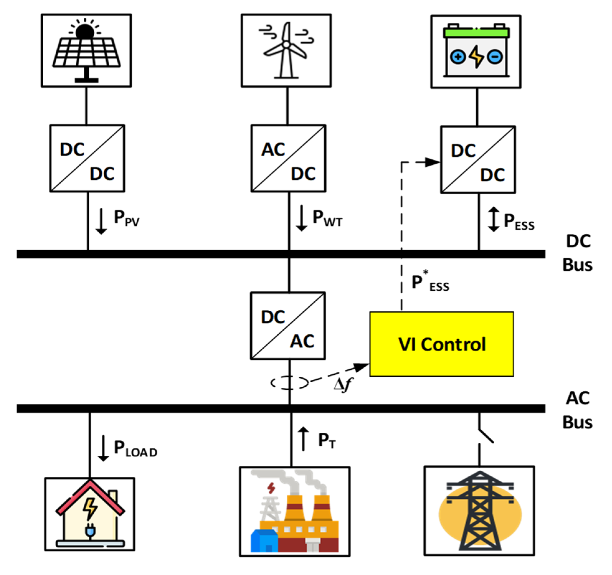
2. System Configuration and Modeling

2.1. Fundamental Frequency Regulation

Frequency regulation is a type of operation in the power grid that involves balancing source power and load power [3]. Frequency regulation involves bringing the frequency back to its normal level whenever a deviation from the nominal value happens. Depending on the cause of the deviation, frequency control is divided into four main operations (as shown in Figure 1), known as primary control, secondary control, tertiary control, and emergency control [3]. When a large frequency deviation occurs, the frequency restoration process typically follows a sequence of response times. Initially, the response occurs with the system’s inertial reaction (0–5 s), followed by primary control (5–10 s), which helps mitigate the rate of frequency decline and stabilize transient fluctuations. Finally, secondary control (20 s–10 min) restores the frequency to its nominal value and ensures long-term stability [4].

Additionally, during normal operation, the system frequency can be adjusted using the inertial response of the generator, helping to reduce small fluctuations. In cases where there is a significant imbalance of power between the load and generator, the inertia response provides support by slowing down the rate of change, allowing other control mechanisms to intervene [22]. In current international standards, the acceptable frequency deviation level typically is within 1% of nominal frequency [4]. This depends on operational conditions, and frequency stability standards may vary among different power grids worldwide. The Australian standard used in this study is ±0.15 Hz in large grid-connected systems, and ±0.5 Hz in off-grid systems [23]. Although traditional frequency control principles play an important role in maintaining the stability of the power system frequency, the development of microgrids with a high proportion of renewable energy sources has significantly changed the dynamic characteristics of the system. In particular, in MGs operating in an islanded mode, the lack of natural rotational inertia from traditional synchronous generators makes the system more sensitive to frequency fluctuations and sudden power fluctuations. Therefore, to better understand the challenges and solutions of frequency control in modern MGs, it is necessary to build and analyze the dynamic model of MGs. The next section will present the system configuration and dynamic modeling of microgrids, which will serve as a foundation for the design of advanced control strategies.

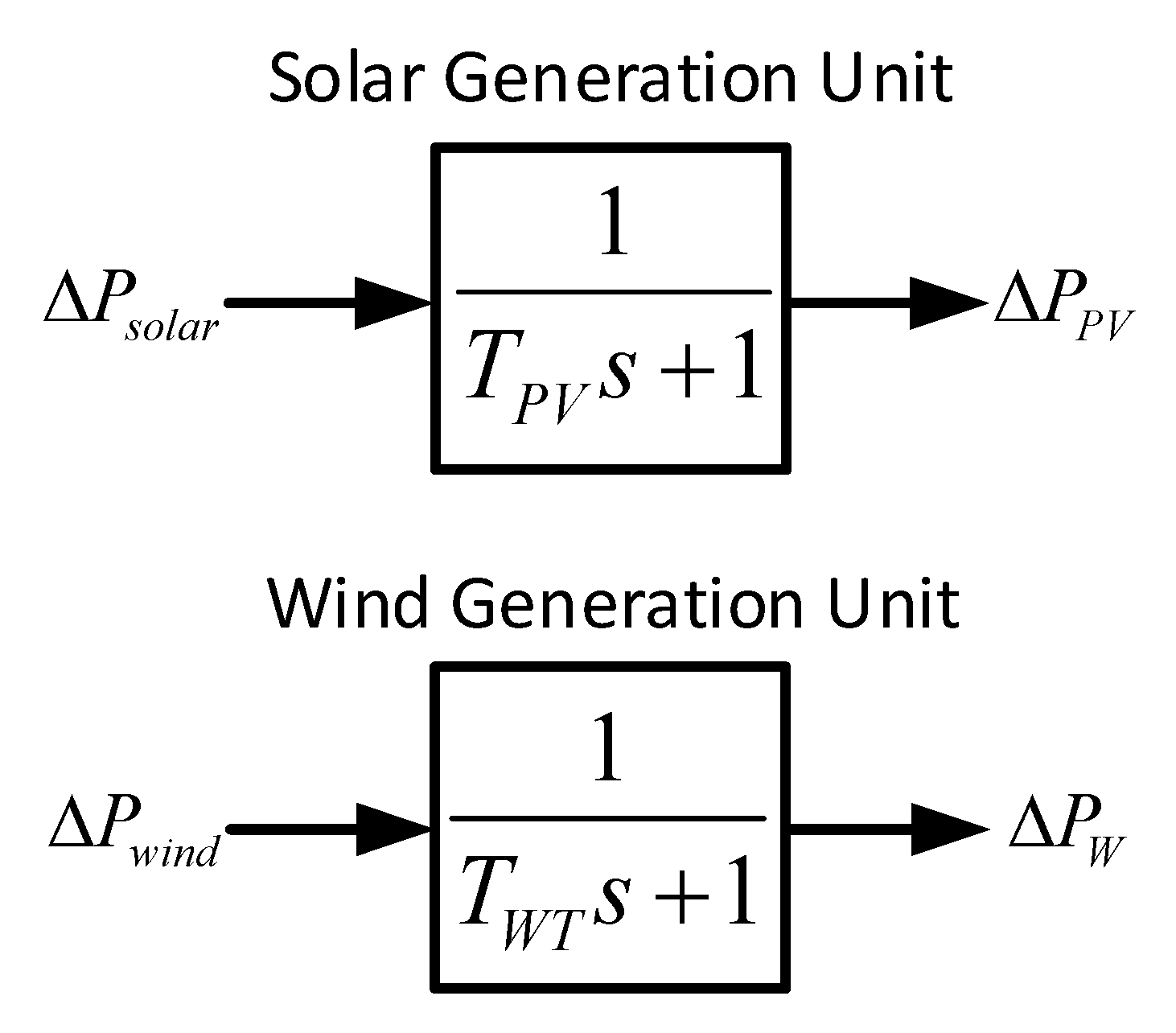
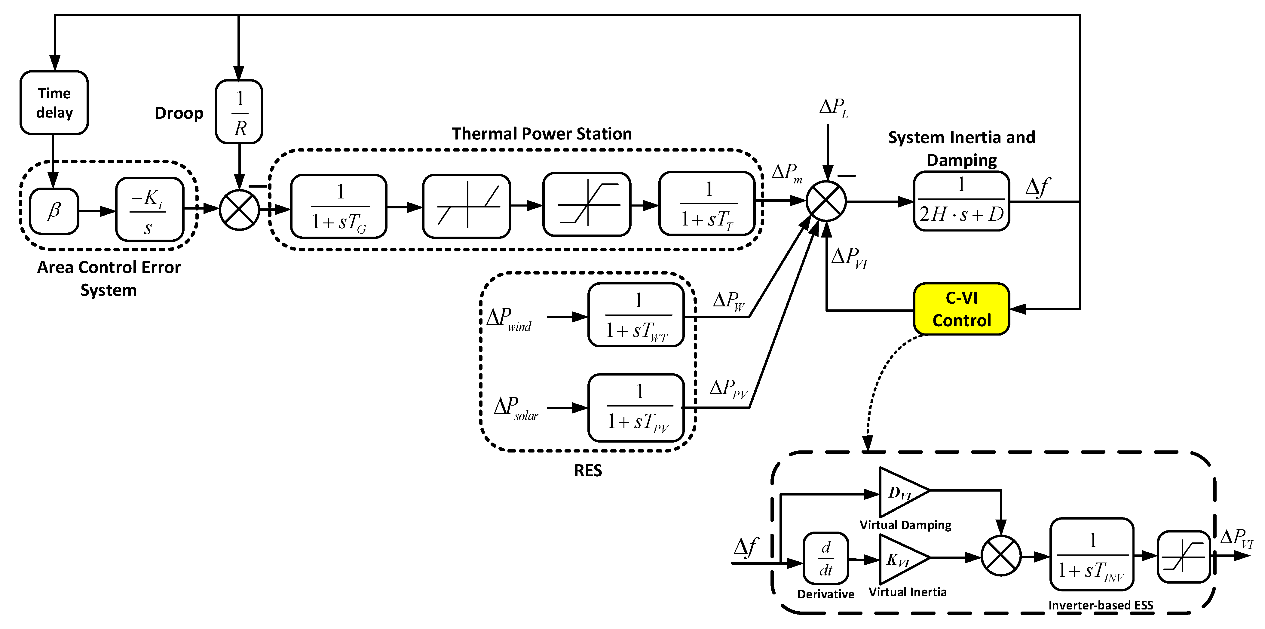
2.2. Microgrid Dynamic and Modeling

The basic architecture of a microgrid is illustrated in Figure 2, consisting of various components such as an energy storage system (ESS), an inverter, a wind power system, a solar power system, an internal combustion engine, a diesel generator, multiple inverters, and DC-DC converters [24]. This simple power system is just used for justifying the efficiency of the proposed method. The dynamic characteristics of a microgrid are highly complex, involving numerous nonlinear differential algebraic equations [25]. Therefore, to facilitate system analysis and controller design, the microgrid control model is often approximated using linearized models of different hierarchical levels [24].

It is assumed that the investigated system operates in an off-grid mode as shown in Figure 2. In this mode, the system itself dispatches the power needed to operate in the area so that the frequency is stable when a large proportion of energy comes from a very large source of renewable energy. The dynamic characteristics of a microgrid follow the generator–load dynamic relationship, considering the incremental mismatch between power and the frequency deviation (Δf), and can be represented by the swing equation as follows [4,26].

$$\Delta P_m(t)-\Delta P_L(t)=2H{\displaystyle \frac{d\Delta f(t)}{dt}}+D\Delta f(t)$$

(1)

where ΔP_m and ΔP_L are mechanical power deviation and load power deviation, respectively, and H is the inertia constant of the power system calculated based on the inertia constant of the synchronous machine calculated from Equation (2).

$$H={\displaystyle \sum _i\frac{\left(H_{SGi}{S}_{SGi}\right)}{S_{MG}}}$$

(2)

where S_SG and S_MG denote the rated power of the synchronous generator and the nominal microgrid system power, respectively. From this assumption, Figure 3 provides a simplified structure of frequency response, focusing on a single generating unit based on Equation (1).

The modeling of RESs, such as wind and solar power systems, is critical for MG modeling. These RES systems, along with associated energy storage units, are often represented using simplified dynamic models. Such models are deemed sufficient for addressing the frequency control challenges in isolated microgrids. The simplified models primarily consider first-order dynamic responses as shown in Figure 4, although it is acknowledged that some RESs might possess high-order dynamics [27]. This approach helps in analyzing how the system responds to various disturbances including wind power, solar irradiation power, and load demands, which are considered as external disturbances to the system’s frequency stability.

From the above assumptions, the mathematical model of MG for frequency response can be represented with all components as shown in Figure 5.

The speed governor in generators of thermal power system in Figure 5 have a big role in restoring frequency response of the system through the primary control loop and secondary control loop [4,16,19]. And these operational dynamics in thermal power system are crucially influenced by certain physical constraints, which are Governor Dead Band (GDB) and Generation Rate Constraint (GRC) [4]. The GRC restricts the rate of change of plant generating unit’s power output, reflecting realistic limitations imposed by the thermal and mechanical properties of the system [28]. And the purpose of the governor’s dead band is to enhance the apparent steady-state speed controls [27]. These settings help ensure the stability and safety of power generation by controlling the rate at which the turbines can respond automatically to changes in demand or operational conditions.

2.3. Conventional Virtual Inertia Control for Islanded Microgrids

Conventional virtual inertia (C-VI) control is a method designed to stabilize modern power systems by virtually synthesizing additional inertia and damping. This approach enables distributed generation (DG) and RESs to contribute effectively to systems with low inertia [5,9,11]. The C-VI control dynamically calculates the power drawn from the ESS to support grid frequency, thereby addressing imbalances between generation and load [4].

The C-VI control mechanism operates seamlessly in both grid-connected and islanded modes, as illustrated in Figure 5 [29]. Its core components include virtual damping (D_VI) and virtual inertia (K_VI) as the control parameters with frequency error and RoCoF as the inputs [27]. These components emulate the inertia and damping properties of synchronous generators, reducing frequency deviations and enhancing system stability under dynamic conditions. The low-pass filter is used to eliminate the noise issue and to obtain the accurate dynamics of inverter-based ESS (i.e., fast response characteristic). The limiter block is implemented to limit the ESS output power, representing the practical power response of the ESS. As a result, the dynamic equation of the C-VI control is expressed as follows:

$$\Delta P_{VI}(s)={\displaystyle \frac{s{K}_{VI}+D_{VI}}{1+s{T}_{INV}}}\Delta f(s)$$

(3)

where T_INV represents the time constant of the inverter-based ESS. Inverters play a central role in the C-VI control scheme, operating either voltage sources or current sources [30]. By employing linearization feedback control, the active and reactive power of the inverter can be adjusted with minimal delay, enabling the inverter to respond to its reference power within a short time [30]. With this fast dynamic response, the inverter dynamic can be modeled as a first-order transfer function [27].

To ensure safe operation and enhance performance, a Power Limiter Unit is connected to the C-VI control structure as shown in Figure 5. This unit imposes upper (P_{INV_max}) and lower (P_{INV_min}) boundaries on the ESS output power. By restricting output power, the power limiter prevents overloading of the inverter and ESS, protects against rapid power fluctuations, and ensures operation within physical constraints. This capability is particularly critical during high renewable energy variability or sudden load changes.

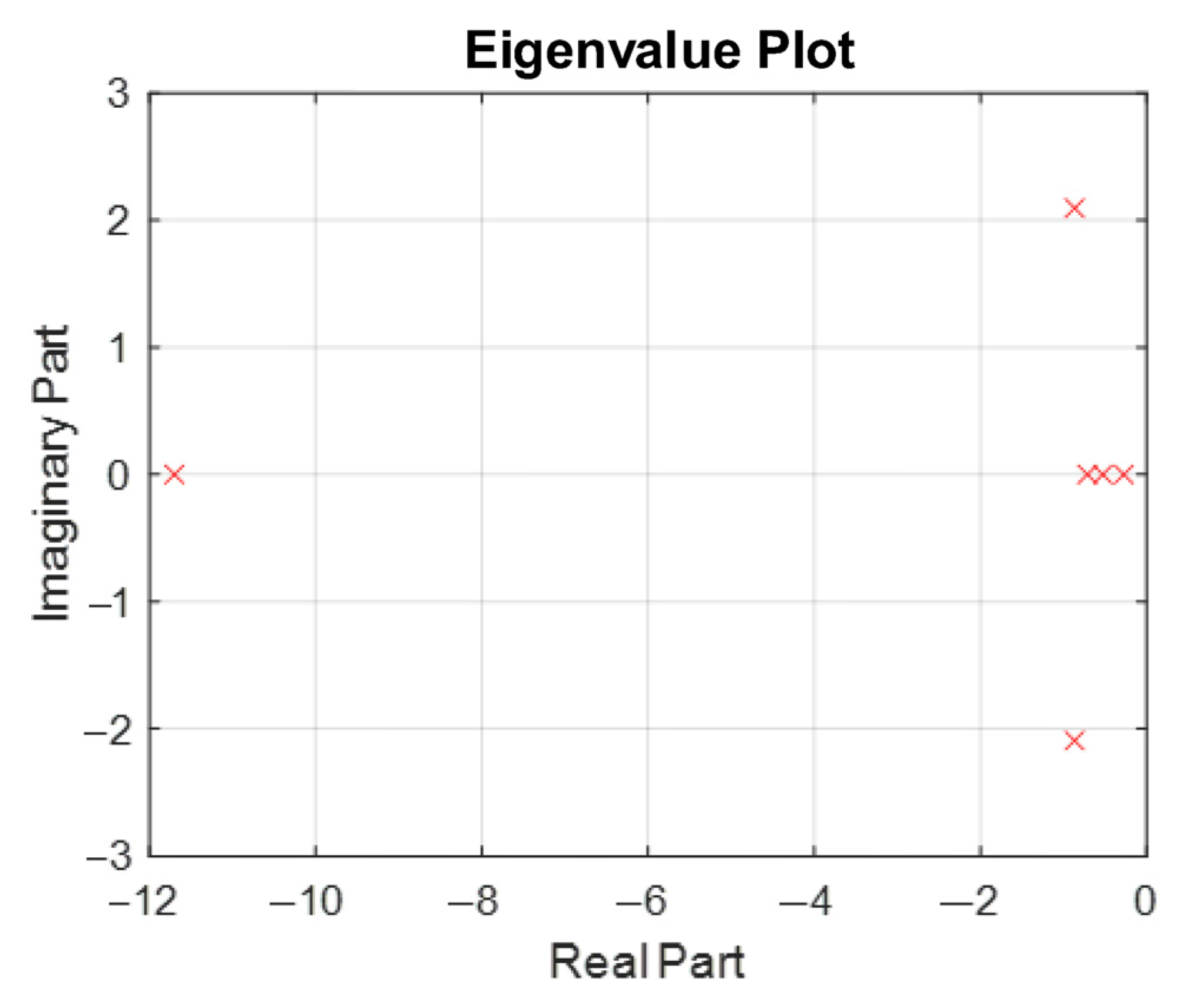
2.4. State-Space Modeling of Microgrid

The use of state-space representation plays an important role in the further analysis of the object model as well as in the application of modern controllers. From the ESS, thermal power system, load, and wind and solar power system modeling mentioned above, the microgrid based on Figure 5 can be expressed in state-space modeling as follows [4].

$$\Delta f={\displaystyle \frac{1}{2Hs+D}}\left(\Delta P_m+\Delta P_W+\Delta P_{PV}+\Delta P_{VI}-\Delta P_L\right)$$

(4)

$$s\Delta P_m(s)=-{\displaystyle \frac{\Delta P_m(s)}{T_t}}+{\displaystyle \frac{\Delta P_g(s)}{T_t}}$$

(5)

$$s\Delta P_g(s)=-{\displaystyle \frac{\Delta f(s)}{R{T}_g}}-{\displaystyle \frac{\Delta P_g(s)}{T_g}}+{\displaystyle \frac{\Delta P_C(s)}{T_g}}$$

(6)

$$s\Delta P_C(s)=-K_S\beta \Delta f(s)$$

(7)

$$s\Delta P_W(s)=-{\displaystyle \frac{\Delta P_W(s)}{T_{WT}}}+{\displaystyle \frac{\Delta P_{wind}(s)}{T_{WT}}}$$

(8)

$$s\Delta P_{PV}(s)=-{\displaystyle \frac{\Delta P_{PV}(s)}{T_{PV}}}+{\displaystyle \frac{\Delta P_{solar}(s)}{T_{PV}}}$$

(9)

Hence, the model can be expressed as this following form:

$$\left\{\begin{array}{l}\stackrel{•}{x(t)}=Ax(t)+B_{1}w(t)+B_{2}u(t)\\ y(t)=Cx(t)\end{array}\right.$$

(10)

where x(t)^T = [Δf ΔP_m ΔP_g ΔP_c ΔP_W ΔP_PV] is the state vector of the model, w^T = [ΔP_wind ΔP_solar ΔP_L] is disturbance vector, and control signal u = ΔP_VI. More specifically, ΔP_c is the power fluctuation from the area control error (ACE) of the secondary control, ΔP_m is the power fluctuation of the thermal power station, ΔP_g is the output power deviation at the governor system, ΔP_W and ΔP_PV are the output power fluctuation of the wind and solar systems, respectively, and ΔP_L is the load power deviation. Substituting Equations from (4)–(9) into the state-space model (10), we have the system of state equations with the following system matrices:

$$A=\left[\begin{array}{cccccc}-{\displaystyle \frac{D}{2H}}& {\displaystyle \frac{1}{2H}}& 0& 0& {\displaystyle \frac{1}{2H}}& {\displaystyle \frac{1}{2H}}\\ 0& -{\displaystyle \frac{1}{T_t}}& {\displaystyle \frac{1}{T_t}}& 0& 0& 0\\ -{\displaystyle \frac{1}{R{T}_g}}& 0& -{\displaystyle \frac{1}{T_g}}& {\displaystyle \frac{1}{T_g}}& 0& 0\\ -K_S\beta & 0& 0& 0& 0& 0\\ 0& 0& 0& 0& -{\displaystyle \frac{1}{T_{WT}}}& 0\\ 0& 0& 0& 0& 0& -{\displaystyle \frac{1}{T_{PV}}}\end{array}\right]$$

(11)

$$B_1=\left[\begin{array}{ccc}0& 0& -{\displaystyle \frac{1}{2H}}\\ 0& 0& 0\\ 0& 0& 0\\ 0& 0& 0\\ {\displaystyle \frac{1}{T_{WT}}}& 0& 0\\ 0& {\displaystyle \frac{1}{T_{PV}}}& 0\end{array}\right]$$

(12)

$$B_2=\left[\begin{array}{c}{\displaystyle \frac{1}{2H}}\\ 0\\ 0\\ 0\\ 0\\ 0\end{array}\right]$$

(13)

$$C=\left[\begin{array}{cccccc}1& 0& 0& 0& 0& 0\end{array}\right]$$

(14)

The mathematical model of the MG (10)–(14) is essential for designing the iterative learning controllers.

3. Designing Iterative Learning Control for Frequency Regulation

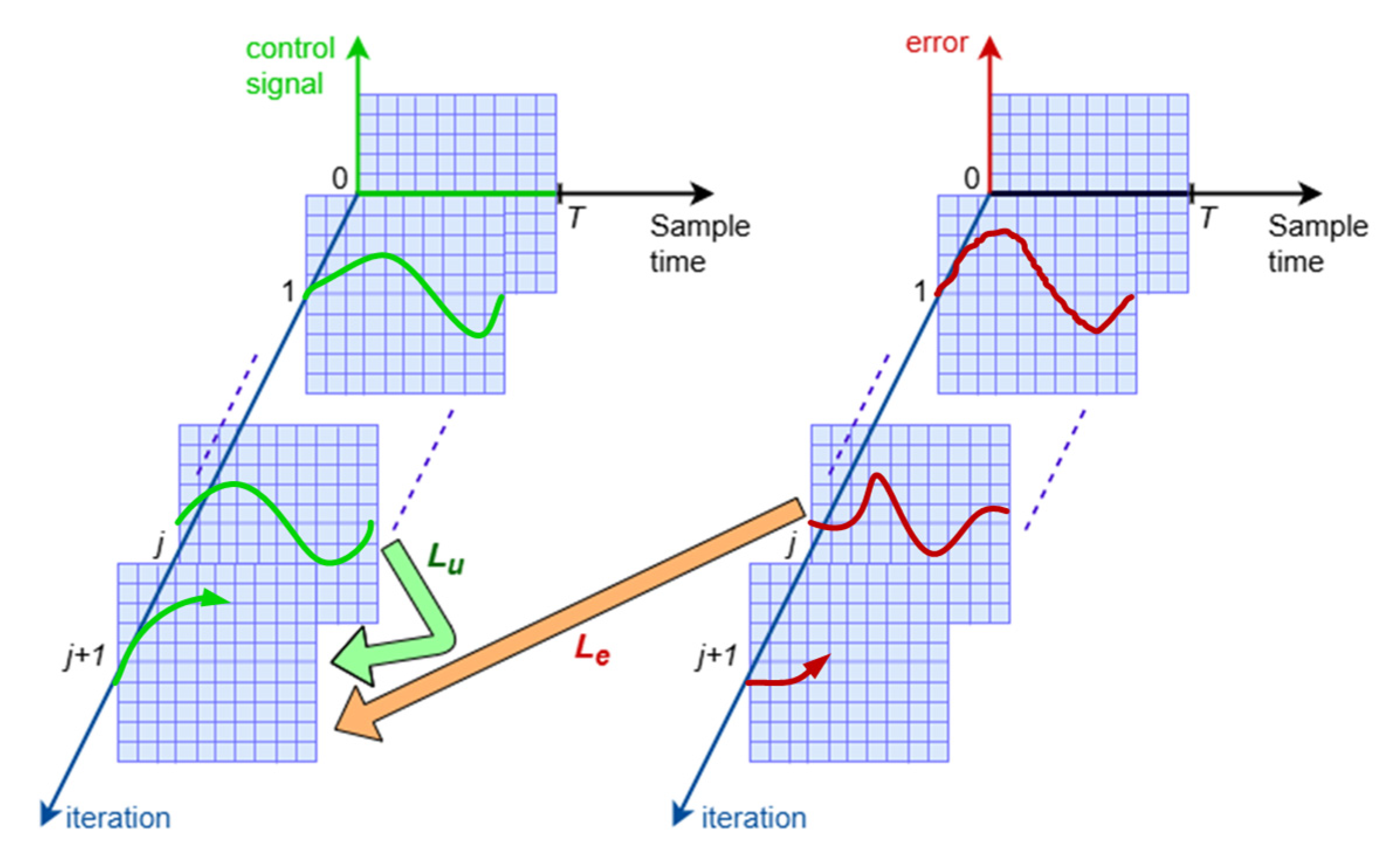
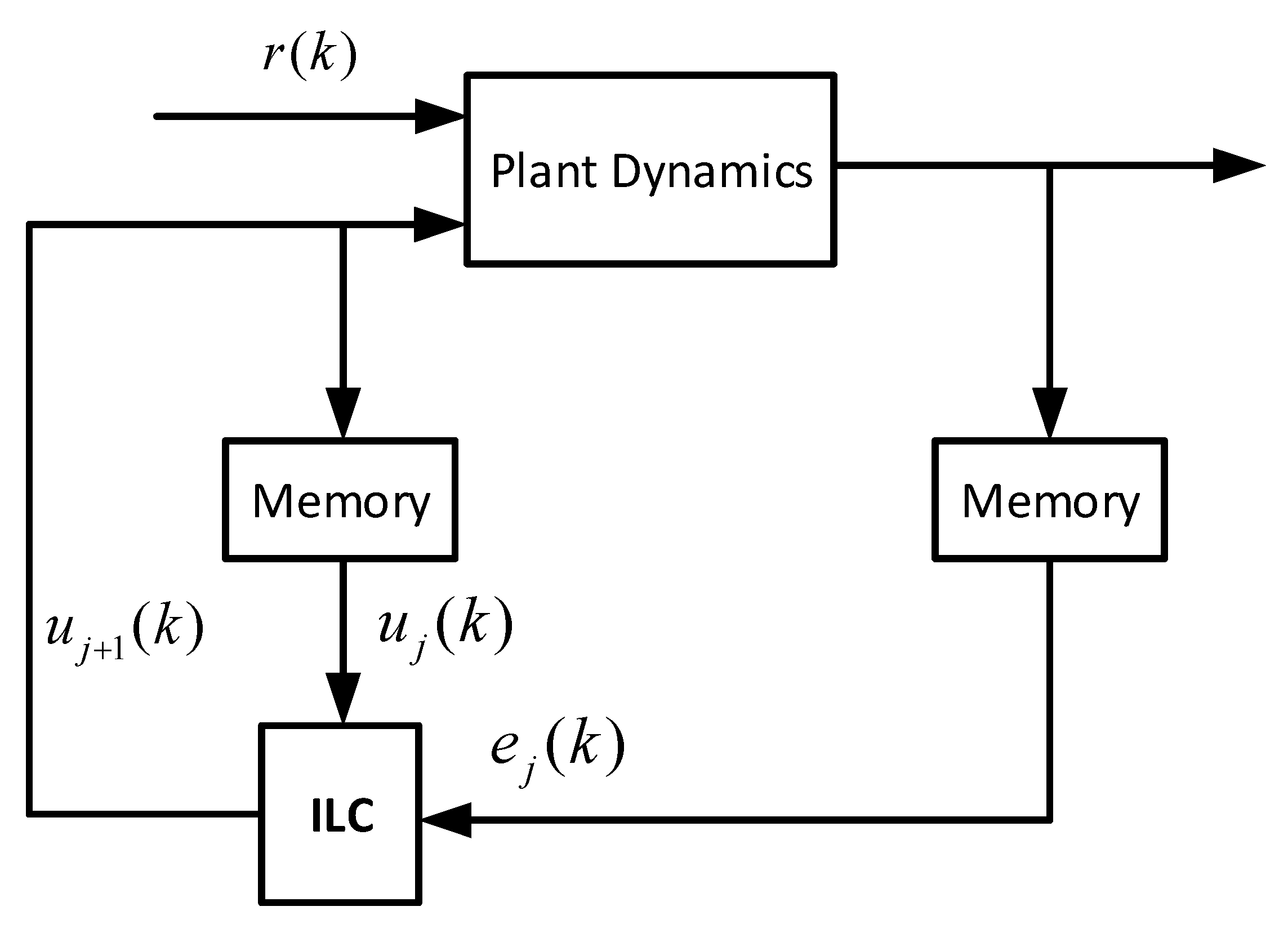
3.1. Basic Concept of Iterative Learning Control

Iterative Learning Control (ILC) is a control technique that uses the control signal from previous iterations, as shown in Figure 6, to improve the current system’s transient response [21]. The objective of this control method is to decrease the error between the response and the reference signal, enabling convergence over iterations.

ILC is considered an intelligent control system because it does not require a complete mathematical model of the system being controlled. This control method can be applied to both continuous and discrete-time systems [21,31]. ILC is most commonly used for discrete-time systems since these systems are typically designed based on discrete control techniques. For ILC to be effectively implemented, the following three conditions must be satisfied [31]:

• The system must incorporate ILC within a fixed time interval;
• In each iteration, ILC must generate an output signal to the same reference setpoint;
• The initial state of each iteration should be reset to the same value.

ILC has two primary structures: open-loop ILC and closed-loop ILC. The open-loop ILC structure is often used, whereas the closed-loop ILC structure is only applied in cases where the system undergoes significant variations, causing instability [21]. The block diagram of ILC operating in the discrete domain is illustrated in Figure 7.

The term r(k) represents the reference signal, y_j(k) is the system output at iteration j, e_j(k) is the error between r(k) and y_j(k), and u_j+1(k) is the control signal at trial j + 1. After each iteration, the updated control signal u_j+1(k) is computed and applied to the system in the next iteration, becoming u_j(k). ILC is classified into several orders, for example, second-order means learning from the earlier two trials. In the scope of this study, the first-order controller model is applied. The first-order ILC control equation is applied with two parameters L_u and L_e. The equation is expressed as follows:

$$u_{j+1}=L_u{u}_j+L_e{e}_j$$

(15)

$$e_j(k)=r(k)-y_j(k)$$

(16)

To design ILC, the mathematical model needs to be represented in the discrete domain.

$$\left\{\begin{array}{l}{x}_j(k+1)=A{x}_j(k)+B{u}_j(k)+d_j(k)\\ y_j(k)=C{x}_j(k)\end{array}\right.;k\in \left[0;N\right]$$

(17)

Rewriting the system model in terms of output:

$$y_j(k)=P{u}_j(k)+d_j(k)$$

(18)

$$\mathrm{Where} y_j=\left[\begin{array}{c}{y}_j(1)\\ ⋮\\ y_j(N)\end{array}\right] , u_j=\left[\begin{array}{c}{u}_j(0)\\ ⋮\\ u_j(N-1)\end{array}\right] , d=\left[\begin{array}{c}{d}_j(0)\\ ⋮\\ d_j(N-1)\end{array}\right]$$

The terms y_j, u_j, and d_j represent the output, input, and noise values of the model at the jth iteration, respectively. The P matrix characterizes the system characteristics and is defined as follows:

$$P=\left[\begin{array}{cccc}CB& 0& \dots & 0\\ CAB& CB& \dots & 0\\ ⋮& ⋮& \ddots & ⋮\\ C{A}^{N-1}B& C{A}^{N-2}B& \dots & CB\end{array}\right]=\left[\begin{array}{cccc}{p}_1& 0& \dots & 0\\ p_2& p_1& \dots & 0\\ ⋮& ⋮& \ddots & ⋮\\ p_N& p_{N-1}& \dots & p_1\end{array}\right]$$

(19)

where A, B, and C are the main-system-describing matrices in equation (17).

The Markov parameters in the P matrix of the system are represented by the system’s state equations or can be obtained from the system’s impulse response matrix (CAⁱ⁻¹B) [32]. The controller equation only depends on two adjustment matrices L_u and L_e. To minimize the error between learning times, convergence must be ensured. The error will converge when L_u and L_e are chosen to satisfy the following conditions [21,32].

$$‖L_u-L_e.P‖<1$$

(20)

3.2. Virtual Inertia Control Based Iterative Learning Control

The ILC learning rules can be combined with conventional controllers such as P-type (i.e., proportional-type) or PD-type (i.e., proportional–derivative-type). PD-type controllers will be examined. For simplicity, the parameters are set as follows:

$$L_u=I$$

(21)

$$L_e=\left[\begin{array}{cccc}{k}_d& 0& 0& 0\\ k_p-k_d& k_d& 0& 0\\ ⋮& \ddots & \ddots & ⋮\\ 0& \dots & k_p-k_d& k_d\end{array}\right]$$

(22)

The control signal will then follow the learning formula at iteration (j + 1) with the PD control law shown in Equation (23).

$$\begin{gathered} u_{j+1}(k)=u_j(k)+k_p{e}_j(k)+k_d(e_j(k+1)-e_j(k)) \\ \Delta u_{j+1}(k)=(k_p+k_d)e_j(k+1)+k_d{e}_j(k) \end{gathered}$$

(23)

where k_p and k_d are real constant gains, and we call them proportional and derivative learning gain of PD-type, respectively. To ensure the convergence condition of Equation (20), the selection of two parameters k_p and k_d is crucial [31,32].

From Equation (16), we obtain the following:

$$e_{j+1}=e_j+y_j-y_{j+1}=e_j-P\Delta u_{j+1}$$

(24)

Matrix F is defined as follows:

$$F=\left[\begin{array}{cccccc}0& 0& 0& \dots & 0& 0\\ 1& 0& 0& \dots & 0& 0\\ 0& 1& 0& & 0& 0\\ ⋮& ⋮& & \ddots & ⋮& ⋮\\ 0& 0& \dots & 1& 0& 0\\ 0& 0& \dots & 0& 1& 0\end{array}\right]$$

(25)

We obtain the following:

$$\begin{array}{l}{G}_c=I-(k_P+k_D)P+k_{D}PF\\ =\left[\begin{array}{cccccc}{g}_{c1}& 0& 0& \dots & 0& 0\\ g_{c2}& g_{c1}& 0& & 0& 0\\ g_{c3}& g_{c2}& g_{c1}& & 0& 0\\ ⋮& & & \ddots & & ⋮\\ g_{c(N-1)}& g_{c(N-2)}& g_{c(N-3)}& & g_{c1}& 0\\ g_{cN}& g_{c(N-1)}& g_{c(N-2)}& \dots & g_{c2}& g_{c1}\end{array}\right]\end{array}$$

(26)

where G_c is a lower triangular Toeplitz matrix formed by vector g_c:

$$g_c=\left[\begin{array}{c}{g}_{c1}\\ g_{c2}\\ g_{c3}\\ ⋮\\ g_{c(N-1)}\\ g_{cN}\end{array}\right]=\left[\begin{array}{c}1-p_1{k}_p-p_1{k}_d\\ -p_2{k}_p-(p_2-p_1)k_d\\ -p_3{k}_p-(p_3-p_2)k_d\\ ⋮\\ -p_{N-1}{k}_p-(p_{N-1}-p_{N-2})k_d\\ -p_N{k}_p-(p_N-p_{N-1})k_d\end{array}\right]$$

(27)

From Equations (24)–(27), we obtain the following:

$$e_{j+1}=G_c{e}_j$$

(28)

The convergence condition of ILC system is given by the following:

$$\underset{j\to \infty }{\lim } e_j=0$$

(29)

According to [33], in order to satisfy convergence condition in Equation (29), all eigenvalues of matrix G_c must be located into the unit circle, which is given by the following:

$$\left|g_{c1}\right|<1\mathrm{or} 0<k_p+k_d<{\displaystyle \frac{2}{p_1}}={\displaystyle \frac{2}{CB}}$$

(30)

During the learning process, the algorithm learns the dynamic characteristics of the system and adjusts the control signals. Therefore, in the PD-type ILC controller, there is no need to identify the system, and it is enough to associate with the first Markov parameter. It gives this type of iterative learning an advantage because of its simplicity [18]. In this study, the ILC method is integrated with a C-VI control to calculate the output power of ESS, which is connected to the microgrid. The goal is to enhance the stability of MG operation. Although the MG model faces constraints, such as inverter output power limit, which is a static nonlinear factor, wind and solar power fluctuations, or large load variations, the ILC method is suitable for these types of models. With the ILC objective mentioned in Section 3.1, it is demonstrated that applying ILC to C-VI control helps reduce the impact of frequency fluctuations as well as RoCoF. Consequently, this contributes to improving the stability of MG operation and MG inertia.

Based on the C-VI controller examination, the structure of C-VI is similar to the PD controller with virtual damping such as k_p (proportional) and the differential term with virtual inertia such as k_d (derivative). This means the combination of ILC and C-VI control is similar to the PD-type ILC controller. Based on the learning rule in Equation (23), the learning law of ILC-VI is indicated as follows:

$$u_j(k+1)=u_j(k)+D_{VI}\Delta f_j(k)+K_{VI}\left(\Delta f_j(k+1)-\Delta f_j(k)\right)$$

(31)

where Δf_j(k) and Δf_j(k + 1) are the frequency responses at time k and k + 1 in jth loop, respectively. With matrix L_u = I, the selection of D_VI and K_VI for L_e similarly to the selection of k_p and k_d, respectively, must satisfy the convergence conditions as in Equation (30). The detailed structure of the ILC-VI controller is shown in Figure 8 and Figure 9.

This control method is suitable as a backup when a fault occurs on the grid. After these learning iterations, the control signal u_j(k) providing the best frequency response quality (in terms of nadir/overshoot frequency and RoCoF) at a given learning trial is stored in the controller memory, and then it used as a control signal whenever the power fluctuation between the source and the load is too large.

4. Simulation Results and Discussions

This section details the simulation results and analysis used to assess the effectiveness of both the traditional VI control and the integrated ILC-VI method in stabilizing the frequency of a low-inertia microgrid. The microgrid was modeled and simulated in MATLAB/Simulink to introduce disturbances and evaluate its dynamic behavior under various conditions. Operating in an islanded mode, the simulated microgrid includes several components depicted in Figure 5: a 9 MW solar farm, a 7 MW wind farm, domestic loads totaling 15 MW, a 1 MW ESS, and a 12 MW thermal power plant. The total system base is 12 MW, providing a diverse mix of generation and load to evaluate the control strategies. The parameters used for simulation are detailed in

Table 1. System parameters.

Symbol	Quantity	Value
Ki	Gain of integral controller	0.1
TG	Governor time constant	0.09 (s)
TT	Turbine time constant	0.4 (s)
R	Governor droop constant	2.6 (Hz/p.u.)
β	Bias factor	0.98 (p.u./Hz)
KVI	Virtual inertia constant	0.2 (p.u. s)
DVI	Virtual damping constant	0.3 (p.u./Hz)
TINV	Time constant of inverter-based ESS	3.0 (s)
TW	Time constant of wind turbine	1.4 (s)
TPV	Time constant of solar system	1.9 (s)
H	Microgrid system inertia	0.083 (p.u. s)
D	Microgrid system damping	0.016 (p.u./Hz)
Lu	Filter parameter of ILC	I
Kp	Proportional gain of ILC	0.11
Kd	Derivative gain of ILC	0.085

[4,19].

The simulation time is set for 200 s. The simulation was performed under two scenarios. To assess the effectiveness of ILC-VI compared to C-VI control, the ILC-VI method was run for seven iterations to explore its learning and adaptation capabilities over repeated trials. Before utilizing the ILC-VI control, the system model needs to be asymptotically stable [34]. For the above parameters and state matrix in Equation (11), the eigenvalues of the matrix are all located to the left side of the complex plane, as depicted in Figure 10. Another stability condition that needs to be considered is that the error between desired output signal and output response must converge to 0. For the convergence analysis, the L_u and L_e parameters must be set so that they satisfy Equation (20); here, we set L_u = I. As for the L_e parameter, K_d = 0.085 and K_p = 0.11. Furthermore, the first Markov parameter CB (or CB₁) is derived from the state-space model in Equation (10), where the output y is the frequency deviation Δf (the first state in the vector x(t) = [Δf, ΔP_m, ΔP_g, ΔP_C, ΔP_W, ΔP_PV]^T), so C = [1, 0, 0, 0, 0, 0]. The input matrix B is given in Equation (12) as B₁ = [${\displaystyle \frac{1}{2H}}$, 0, 0, 0, 0, 0]^T, with H = 0.083 p.u.s from Table 1. Thus, $CB=p_1={\displaystyle \frac{1}{2H}}={\displaystyle \frac{1}{2\times 0.083}}\approx 6.024$. Therefore, in this model, $\left|g_{c1}\right|=\left|1-p_1(K_P+K_d)\right|=\left|1-6.024(0.11+0.085)\right|=\left|-0.174\right|=0.174<1$, which satisfies the stability condition in Equation (30) as derived in Section 3.2. Quantitative convergence criteria are defined as monotonic error reduction, ensuring $\left|g_{c1}\right|<1$, beyond the visual inspection of frequency response curves; this guarantees asymptotic stability and minimizes steady-state error across iterations, as validated by reductions in RoCoF and frequency nadir in simulations.

4.1. Scenario 1: Unit Step Load Power and Constant RES Power

In this case study, load power undergoes fluctuations through unit step responses in load power deviation at time points of 10 and 100 s as shown in Figure 11. When there is no fluctuation in RESs, the RES power deviation is 0 throughout the simulation.

The frequency response of the iterations is shown in Figure 12. The ILC-VI control significantly improves the dynamic response over iterations. As iterations progress, the ILC-VI control demonstrates significant improvements in dynamic performance. From these iterations, the fifth iteration was selected for detailed analysis, as it consistently delivers a superior output response, specifically in terms of frequency nadir, overshoot, and RoCoF, compared to C-VI, while maintaining a settling time within an acceptable range, though not necessarily shorter than that of C-VI. Following the load power deviation increase to 0.08 p.u at 10 s, the frequency deviation nadir (the minimum frequency reached during the transient) improves from approximately −0.22 Hz under the C-VI control to −0.16 Hz by the fifth iteration of ILC-VI. At the load decrease at 100 s, the frequency deviation overshoot is reduced from 0.47 Hz (C-VI) to 0.41 Hz. Additionally, the RoCoF decreases from 0.368 Hz/s in the C-VI case to 0.361 Hz/s in the fifth iteration after the load increases, and from 0.752 Hz/s to 0.729 Hz/s after the load decreases, indicating a smoother transient response. However, a trade-off is observed with the increase in settling time with each iteration. Choosing which iteration has the desired output response is important. The fifth iteration was selected as optimal based on quantitative criteria: it achieves a 27% reduction in frequency nadir (from −0.22 Hz to −0.16 Hz) and a 3% decrease in RoCoF (from 0.368 Hz/s to 0.361 Hz/s) compared to C-VI, while balancing performance gains against computational burden—further iterations increase oscillations without proportional benefits, as seen in the gradual convergence of metrics in

Table 2. Simulation results.

Scenario			Frequency Nadir/Overshoot (Hz)	RoCoF (Hz/s)	Settling Time (s)
1	10 s	C-VI	−0.22	0.368	35.4
		ILC-VI (5th trial)	−0.16	0.361	35.7
	100 s	C-VI	0.47	0.752	60
		ILC-VI (5th trial)	0.41	0.729	40.3
2	10 s	C-VI	0.251	0.125	45
		ILC-VI (5th trial)	0.2	0.11	43
	100 s	C-VI	−0.553	0.242	50.5
		ILC-VI (5th trial)	−0.441	0.231	47.4

. The stored control signal from the fifth iteration of ILC-VI, which provides the optimal frequency response, can be reused for similar load disturbance patterns, enhancing the controller’s practicality.

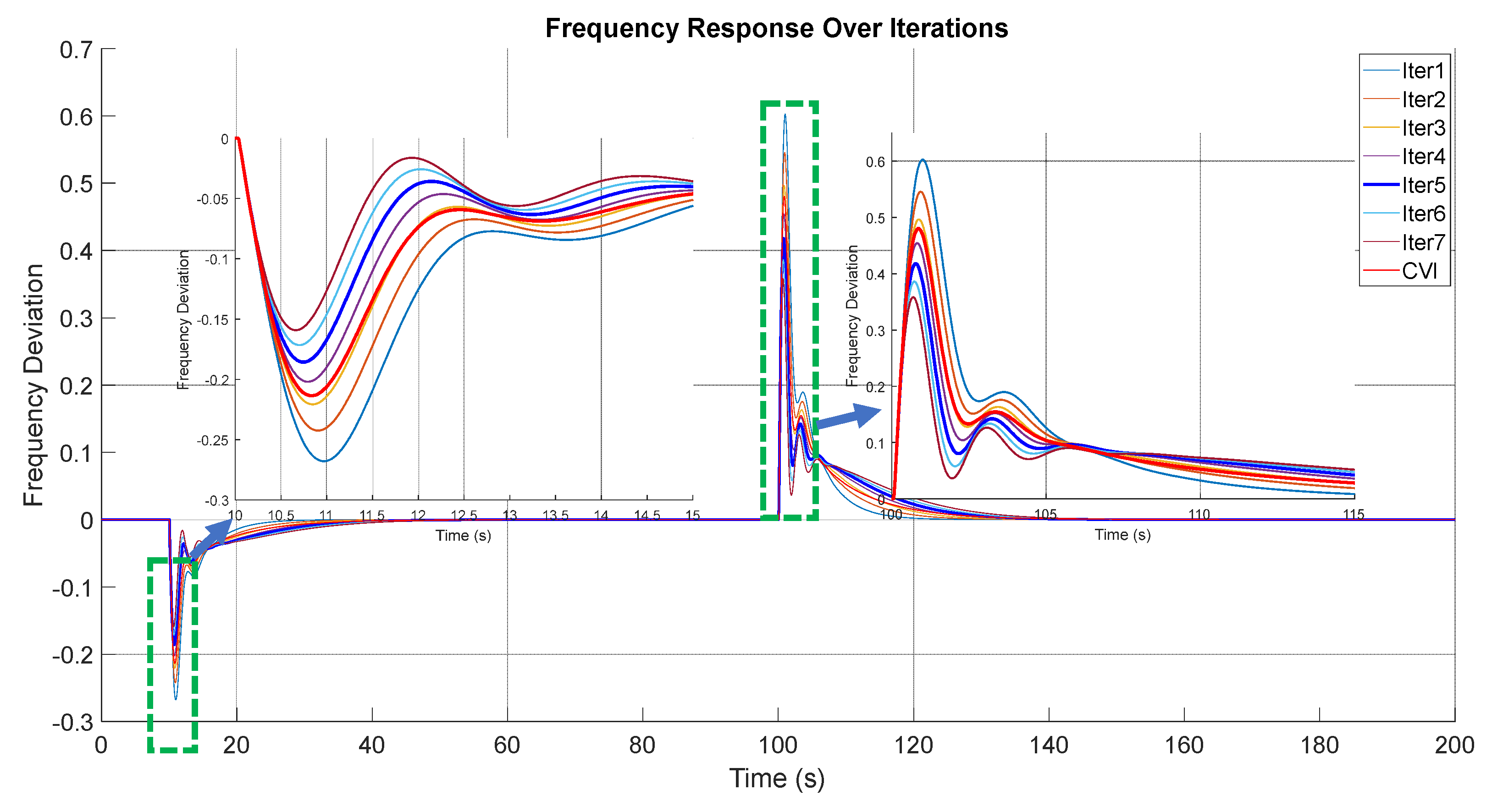
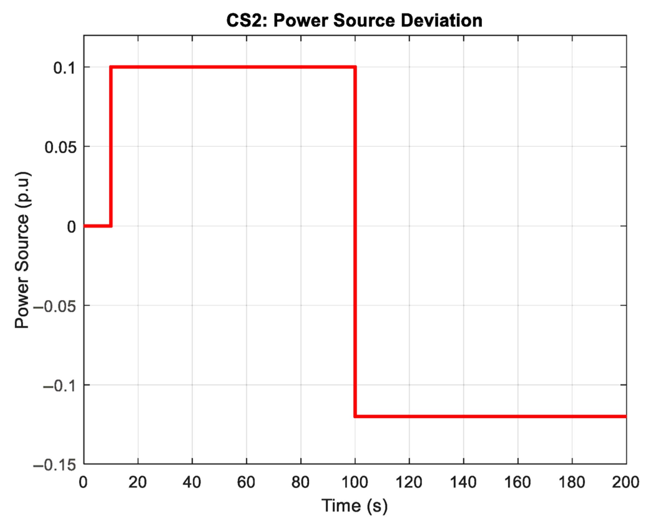
4.2. Scenario 2: Unit Step RES Power and Constant Load Power

There are no fluctuations in load power in this scenario; therefore, the load power deviation appears to be 0 during the simulation time. However, to present the intermittence of RESs, RES power (wind and solar) experiences unit step changes. Specifically, a step increase of 0.1 p.u. in RES power deviation occurs at 10 s, followed by a step decrease to −0.12 p.u. in solar power deviation at 100 s as shown in Figure 13.

The frequency response under this scenario is illustrated in Figure 14. The traditional VI control (C-VI) exhibits a frequency overshoot of 0.251 Hz following the RES power increase and a nadir of −0.553 Hz after the RES power decrease. The RoCoF reaches 0.125 Hz/s and 0.242 Hz/s, respectively, indicating significant transient fluctuations. In contrast, the ILC-VI control improves these metrics iteratively. By the fifth iteration, the frequency overshoot reduces to 0.2 Hz, the nadir increases to −0.441 Hz, and the RoCoF decreases to 0.11 Hz/s and 0.231 Hz/s, respectively. These improvements highlight the adaptive learning capability of ILC-VI, which leverages historical data to mitigate the impact of RES variability. Table 2 provides a detailed comparison of key performance metrics for Scenarios 1 and 2.

According to Table 2, the interval between nadir frequency values and RoCoF between iterations gradually decreases. The settling time for each iteration also shortens as the number of iterations increases, indicating improved convergence. When the frequency nadir and RoCoF values meet the control requirements, the settling time is converged and cannot be reduced further. However, this does not mean that more iterations are always better, as an excessive number of iterations can negatively impact control effectiveness. Figure 12 and Figure 14 also illustrate that the total oscillation of the output response increases as the number of iterations grows. In terms of grid code requirements, ILC delivers frequency response that meets Australian frequency deviation limit quality standards for the islanded grid (±0.5 Hz) [23]. Besides choosing the appropriate iteration, selecting optimal controller parameters of ILC-VI is also important, and this leads to a more stable, reasonable response, and convergence is achieved faster [21,31]. Thus, optimal parameter tunning approaches have been developed in previous studies [32,35]. These results confirm the advantages of integrating ILC into the C-VI control for systems with low inertia, particularly when experiencing high renewable energy fluctuations.

4.3. Parameter Selection Methodology and Sensitivity Analysis

The selection of K_p = 0.11 and K_d = 0.085 was based on empirical tuning to balance convergence speed and system stability, ensuring $\left|g_{c1}\right|<1$ while minimizing frequency nadir and RoCoF in simulations. To illustrate the impact of variations in K_p and K_d, a sensitivity analysis was conducted by varying each parameter around the nominal values (e.g., ±20%), while keeping the other fixed, and evaluating key performance metrics (frequency nadir, RoCoF, and settling time) under Scenario 1 (unit step load at 10 s).

Table 3. Simulation results with different parameter changes.

Parameter Variation	Kp	Kd	$\left|{\mathit{g}}_{\mathit{c}1}\right|$	Frequency Nadir (Hz)	RoCoF (Hz/s)	Settling Time (s)
Nominal	0.11	0.085	0.174	−0.16	0.361	35.7
Kp + 20%	0.132	0.085	0.246	−0.154	0.355	34.2
Kp − 20%	0.088	0.085	0.102	−0.18	0.368	37.1
Kd + 20%	0.11	0.102	0.209	−0.155	0.358	35.0
Kd − 20%	0.11	0.068	0.139	−0.165	0.364	36.5

summarizes the results.

Increasing K_p or K_d tightens the convergence margin ($\left|g_{c1}\right|$ increases but remains < 1), leading to faster convergence (a lower settling time) and improved nadir/RoCoF, but excessive increases (e.g., >30%) could push $\left|g_{c1}\right|$ > 1, causing divergence. Decreasing them widens the margin but degrades performance, increasing oscillations. This analysis confirms that the nominal values provide an optimal trade-off for robustness against load disturbances, with $\left|g_{c1}\right|$ safely below 1. In another context, if the value of CB = 0, the convergence condition is violated, and there are no parameters K_p or K_d that satisfy the convergence condition (20). In this case, instead of determining K_p and K_d according to the convergence condition (20), we can determine K_p and K_d according to some optimality criterion, which is appropriately chosen, such as the following:

$$K=\arg \min ‖e_{j+1}‖, e_{j+1}=G_c(\mathrm{z}).{\mathrm{e}}_j$$

(32)

The matrix $G_c(\mathrm{z})$ contains elements $g_{ij}$ that depend on the constraint $z$.

($z_{\min }<z<z_{\max }$) is as follows:

$$g_{ij}=\left\{\begin{array}{c}0\hspace{1em}if \mathrm{i}<\mathrm{j}\\ 1-CB(z_1+z_2)\hspace{1em}if \mathrm{i}=\mathrm{j}\\ -C{A}^{i-j}\mathrm{B}{\mathrm{z}}_1+(C{A}^{i-j}\mathrm{B}-C{A}^{i-j-1}\mathrm{B}){\mathrm{z}}_2\hspace{1em}if \mathrm{i}>\mathrm{j}\end{array}\right.$$

(33)

This is an example of a suitable optimal criterion, because in order to have the sum of squared errors in the previous trial smaller than in the next trial, according to the convergence condition (20), it must satisfy Equation (32). Constraints $z_1$ and $z_2$ are experimental constraints that depend on the designer experiences.

4.4. Discussion on Complex Scenarios, Scalability, and Implementation

The selection of Scenarios 1 and 2, featuring step changes in load and RES power, is motivated by their representation of worst-case phenomena in microgrids, such as sudden imbalances that maximize frequency deviations and RoCoF, allowing the rigorous evaluation of controller robustness under extreme conditions; by demonstrating improvements in these worst-case scenarios, the ILC-VI method ensures reliable performance and effective mitigation under more typical, less severe disturbances like gradual noise or minor fluctuations. For more realistic disturbances, such as random fluctuations in wind and solar irradiance with time-varying profiles, the ILC-VI controller is expected to perform robustly due to its iterative learning mechanism. Unlike fixed-parameter controllers like C-VI, ILC-VI learns from previous iterations to optimize the control signal, making it particularly suitable for repetitive or quasi-periodic disturbances common in renewable energy sources (e.g., diurnal solar patterns or stochastic wind variations). In simulations with random profiles (e.g., noise superimposed on irradiance data), ILC-VI would likely reduce frequency nadir and RoCoF over iterations by adapting to the disturbance patterns, as inferred from similar studies on ILC in dynamic systems [21,32]. However, initial iterations might show higher transients under highly non-repetitive noise, requiring a sufficient number of learning cycles for convergence. Under multiple simultaneous disturbances, such as combined load changes and RES fluctuations (e.g., a sudden load increase coinciding with a drop in solar output), ILC-VI’s ability to minimize error through accumulated knowledge would help mitigate compounded effects. For instance, the controller could store optimal signals from prior combined events, reducing RoCoF by learning to balance virtual inertia and damping dynamically. Continuous dynamic variations, rather than discrete step changes, would further highlight ILC-VI’s strengths, as the method excels in tracking smooth trajectories over time, potentially leading to lower steady-state errors in long-duration simulations.

Regarding scalability, the ILC-VI method is well suited for larger microgrids with higher renewable penetration. As system size increases, the state-space model can be extended to include more distributed generators, with CB recalculated based on inertia (H). The learning process remains computationally similar per iteration, but convergence speed may improve with more data from diverse sources, enhancing robustness against widespread disturbances.

Finally, on computational requirements, the ILC-VI controller is feasible for real-time implementation due to its simple PD-type structure and low-order computations. Each iteration involves basic matrix operations. On standard hardware like embedded microcontrollers, this requires minimal resources, making it suitable for inverter-based ESS without high-end processors. Memory storage for control signals (e.g., seven iterations) is also modest, though real-time adaptations may need hybrid online–offline learning to handle non-repetitive events. Regarding hardware implementation limitations, the modeling of the ESS inverter as a first-order system (Equation (3)) provides a simplified representation for analysis, but it may overlook real-world dynamics that impact performance, as detailed in [4]. For instance, switching delays in the inverter can introduce lags in the control response, potentially exacerbating frequency oscillations during rapid disturbances, while dead-time in PWM switching might cause voltage distortion and harmonic issues, reducing the accuracy of virtual inertia emulation under high-load conditions. Moreover, current-limiting behavior during faults or overloads could restrict the inverter’s output, limiting the effective inertia support and risking instability if not mitigated. Communication latency between system components, such as delays in frequency measurements or control signals, could further influence the ILC learning process by introducing errors in iterative updates, potentially slowing convergence or causing divergence in highly dynamic scenarios. To address these constraints, future work could explore advanced inverter modeling techniques, such as incorporating higher-order dynamics or adaptive control strategies to compensate for delays and distortions, enhancing real-time robustness in hardware-in-the-loop implementations [4].

In summary, the ILC-VI controller used for virtual inertia control strategies results in a reduced RoCoF. However, using fixed C-VI parameters does not guarantee optimal system performance across different scenarios. For instance, these parameters may fail to provide variable inertia during disturbances, limiting the ability to enhance transient stability by leveraging the energy storage system’s transient energy variations. Additionally, they may not sufficiently improve dynamic and transient stability during significant disturbances. Therefore, to enhance system inertia and enable adaptive responses to disturbances—especially under conditions of high renewable energy penetration—further improvements are needed, and our control strategies are based on the PD-type ILC controller, in which, input signal for inverter-based ESS is calculated based on frequency errors. The coefficients K_p and K_d provide a suitable tuning parameter for the iterative learning process. Furthermore, the ILC-VI approach shows promise for scaling to more complex and larger microgrid scenarios

5. Conclusions

In this study, the ILC-VI controller is applied in the virtual inertia control loop to support frequency stability in low-inertia microgrids. The ILC-VI controller ensures the convergence of the learning process while providing good transient performance. The results indicate that the ILC-VI controller minimizes the impact of RES power fluctuations and load variations, thereby improving both the performance and stability of the system. This is particularly important for microgrids with a high integration of renewable energy, where frequency stability is a major concern. However, in the ILC-VI controller, the parameters L_u and L_e are selected experimentally based on the system characteristics and the convergence condition for the desired setpoint. Future research could explore optimal parameter tuning via a linear–quadratic (LQ) design to enhance the convergence speed and robustness, integrating sensitivity analysis for K_p and K_d under varying RES penetration, as suggested in the virtual inertia synthesis literature. The simulation results of this study can be considered a foundation for further improvements in microgrid control strategies. Future work will also focus on experimental validations under complex disturbances, optimizing computational efficiency for real-time scalability, and addressing hardware constraints like inverter delays and communication latency to ensure practical deployment.

References

1. Ulbig, A.; Borsche, T.S.; Andersson, G. Analyzing rotational inertia, grid topology and their role for power system stability. IFAC-PapersOnLine 2015, 48, 541–547. [Google Scholar] [CrossRef]
2. Duong, M.Q.; Tran, N.T.N.; Sava, G.N.; Leva, S.; Mussetta, M. The Impact of 150 MWp PhoAn Solar Photovoltaic Project into Vietnamese QuangNgai-Grid. In Proceedings of the 2018 International Conference and Exposition on Electrical and Power Engineering (EPE), Iasi, Romania, 18–19 October 2018. [Google Scholar]
3. Bevrani, H. Robust Power System Frequency Control; Springer: New York, NY, USA, 2014. [Google Scholar]
4. Kerdphol, T.; Rahman, F.S.; Watanabe, M.; Mitani, Y. Virtual Inertia Synthesis and Control; Springer International Publishing: Cham, Switzerland, 2021. [Google Scholar]
5. Moore, P.; Alimi, O.A.; Abu-Siada, A. A Review of System Strength and Inertia in Renewable-Energy-Dominated Grids: Challenges, Sustainability, and Solutions. Challenges 2025, 16, 12. [Google Scholar] [CrossRef]
6. Bevrani, H.; Ise, T.; Miura, Y. Virtual synchronous generators: A survey and new perspectives. Int. J. Electr. Power Energy Syst. 2014, 54, 244–254. [Google Scholar] [CrossRef]
7. Harasis, S. Controllable transient power sharing of inverter-based droop controlled microgrid. Int. J. Electr. Power Energy Syst. 2024, 155, 109565. [Google Scholar] [CrossRef]
8. Su, Z.; Yang, G.; Yao, L. Transient Frequency Modeling and Characteristic Analysis of Virtual Synchronous Generator. Energies 2025, 18, 1098. [Google Scholar] [CrossRef]
9. Harasis, S.; Sozer, Y. Improved Transient Frequency Stabilization of Grid Feeding Distributed Generation Systems Using Active Damping Control. In Proceedings of the 2019 IEEE Energy Conversion Congress and Exposition (ECCE), Baltimore, MD, USA, 29 September–3 October 2019. [Google Scholar]
10. Nguyen, V.T.; Nguyen, H.V.P.; Truong, T.B.T.; Truong, Q.V. A virtual synchronous generator control method in microgrid with vehicle-to-grid system. J. Electr. Eng. 2023, 74, 492–502. [Google Scholar] [CrossRef]
11. Hesse, R.; Turschner, D.; Beck, H.P. Microgrid stabilization using the Virtual Synchronous Machine (VISMA). In Proceedings of the International Conference on Renewable Energies and Power Quality (ICREPQ’09), Valencia, Spain, 15–17 April 2009. [Google Scholar]
12. Shadoul, M.; Ahshan, R.; AlAbri, R.S.; Al-Badi, A.; Albadi, M.; Jamil, M.A. A comprehensive review on a virtual-synchronous generator: Topologies, control orders and techniques, energy storages, and applications. Energies 2022, 15, 8406. [Google Scholar] [CrossRef]
13. Sakimoto, K.; Miura, Y.; Ise, T. Stabilization of a power system with a distributed generator by a Virtual Synchronous Generator function. In Proceedings of the 8th International Conference on Power Electronics—ECCE Asia, Jeju, Republic of Korea, 30 May–3 June 2011. [Google Scholar]
14. Tamrakar, U.; Shrestha, D.; Maharjan, M.; Bhattarai, B.P.; Hansen, T.M.; Tonkoski, R. Virtual inertia: Current trends and future directions. Appl. Sci. 2017, 7, 654. [Google Scholar] [CrossRef]
15. Kerdphol, T.; Rahman, F.S.; Mitani, Y.; Hongesombut, K.; Küfeoğlu, S. Virtual Inertia Control-Based Model Predictive Control for Microgrid Frequency Stabilization Considering High Renewable Energy Integration. Sustainability 2017, 9, 773. [Google Scholar] [CrossRef]
16. Saleh, A.; Hasanien, H.M.; Turky, R.A.; Turdybek, B.; Alharbi, M.; Jurado, F.; Omran, W.A. Optimal Model Predictive Control for Virtual Inertia Control of Autonomous Microgrids. Sustainability 2023, 15, 5009. [Google Scholar] [CrossRef]
17. Zaid, S.A.; Bakeer, A.; Magdy, G.; Albalawi, H.; Kassem, A.M.; El-Shimy, M.E.; AbdelMeguid, H.; Manqarah, B. A New Intelligent Fractional-Order Load Frequency Control for Interconnected Modern Power Systems with Virtual Inertia Control. Fractal Fract. 2023, 7, 62. [Google Scholar] [CrossRef]
18. Kerdphol, T.; Rahman, F.S.; Mitani, Y.; Watanabe, M.; Küfeoǧlu, S.K. Robust Virtual Inertia Control of an Islanded Microgrid Considering High Penetration of Renewable Energy. IEEE Access 2018, 6, 625–636. [Google Scholar] [CrossRef]
19. Saleh, A.; Omran, W.A.; Hasanien, H.M.; Tostado-Véliz, M.; Alkuhayli, A.; Jurado, F. Manta Ray Foraging Optimization for the Virtual Inertia Control of Islanded Microgrids Including Renewable Energy Sources. Sustainability 2022, 14, 4189. [Google Scholar] [CrossRef]
20. Skiparev, V.; Machlev, R.; Chowdhury, N.R.; Levron, Y.; Petlenkov, E.; Belikov, J. Virtual Inertia Control Methods in Islanded Microgrids. Energies 2021, 14, 1562. [Google Scholar] [CrossRef]
21. Gunnarsson, S.; Norrlöf, M. A Short Introduction to Iterative Learning Control; Linköping University Electronic Press: Linköping, Sweden, 1997. [Google Scholar]
22. Deng, X.; Mo, R.; Wang, P.; Chen, J.; Nan, D.; Liu, M. Review of RoCoF Estimation Techniques for Low-Inertia Power Systems. Energies 2023, 16, 3708. [Google Scholar] [CrossRef]
23. Fang, J.; Li, H.; Tang, Y.; Blaabjerg, F. On the Inertia of Future More-Electronics Power Systems. IEEE J. Emerg. Sel. Top. Power Electron. 2019, 7, 2130–2146. [Google Scholar] [CrossRef]
24. Mishra, S.; Sahu, P.R.; Prusty, R.C.; Panda, S.; Ustun, T.S.; Onen, A. Application of Enhanced Self-Adaptive Virtual Inertia Control for Efficient Frequency Control of Renewable Energy-Based Microgrid System Integrated with Electric Vehicles. IEEE Access 2025, 13, 43520–43531. [Google Scholar] [CrossRef]
25. Hu, W.; Wu, Z.; Dinavahi, V. Dynamic Analysis and Model Order Reduction of Virtual Synchronous Machine Based Microgrid. IEEE Access 2020, 8, 106585–106600. [Google Scholar] [CrossRef]
26. Hamanah, W.M.; Shafiullah, M.; Alhems, L.M.; Alam, M.S.; Abido, M.A. Realization of Robust Frequency Stability in Low-Inertia Islanded Microgrids with Optimized Virtual Inertia Control. IEEE Access 2024, 12, 58208–58221. [Google Scholar] [CrossRef]
27. Kerdphol, T.; Rahman, F.S.; Watanabe, M.; Mitani, Y.; Turschner, D.; Beck, H.-P. Enhanced virtual inertia control based on derivative technique to emulate simultaneous inertia and damping properties for microgrid frequency regulation. IEEE Access 2019, 7, 14422–14433. [Google Scholar] [CrossRef]
28. Morsali, J.; Zare, K.; Hagh, M.T. Appropriate generation rate constraint (GRC) modeling method for reheat thermal units to obtain optimal load frequency controller (LFC). In Proceedings of the 2014 5th Conference on Thermal Power Plants (CTPP), Tehran, Iran, 10–11 June 2014. [Google Scholar]
29. Shobug, M.A.; Chowdhury, N.A.; Hossain, M.A.; Sanjari, M.J.; Lu, J.; Yang, F. Virtual Inertia Control for Power Electronics-Integrated Power Systems: Challenges and Prospects. Energies 2024, 17, 2737. [Google Scholar] [CrossRef]
30. Yazdani, A.; Iravani, R. Voltage-Sourced Converters in Power Systems: Modeling, Control, and Applications; John Wiley & Sons: Hoboken, NJ, USA, 2010. [Google Scholar]
31. Lee, J.H.; Lee, K.S. Iterative learning control applied to batch processes: An overview. Control Eng. Pract. 2007, 15, 1306–1318. [Google Scholar] [CrossRef]
32. Estakhrouieh, M.R.; Gharaveisi, A.A. Optimal iterative learning control design for generator voltage regulation system. Turk. J. Electr. Eng. Comput. Sci. 2013, 21, 1909–1919. [Google Scholar] [CrossRef]
33. Reza-Alikhani, H.-R.; Madady, A. Monotonic convergence conditions in PD type iterative learning control. In Proceedings of the 2011 19th Mediterranean Conference on Control & Automation (MED), Corfu, Greece, 20–23 June 2011. [Google Scholar]
34. Bristow, D.A.; Tharayil, M.; Alleyne, A.G. A survey of iterative learning control. IEEE Control Syst. Mag. 2006, 26, 96–114. [Google Scholar]
35. Longman, R.W.; Liu, S.; Elsharhawy, T.A. A Method to Speed Up the Convergence of Iterative Learning Control for High Precision Repetitive Motion. In Proceedings of the AIAA/AAS Astrodynamics Specialist Conference, Big Sky, MT, USA, 13–17 August 2023. [Google Scholar]
Figure 1. Operations for managing frequency deviations of varying magnitudes.
Sustainability 17 06727 g001
Figure 2. Hybrid microgrid with virtual inertia controller.
Sustainability 17 06727 g002
Figure 3. Structure of microgrid for frequency control.
Sustainability 17 06727 g003
Figure 4. Low-order dynamic model of renewable energy generation unit.
Sustainability 17 06727 g004
Figure 5. The islanded microgrid dynamic model.
Sustainability 17 06727 g005
Figure 6. Illustration of the ILC method.
Sustainability 17 06727 g006
Figure 7. Control structure of ILC.
Sustainability 17 06727 g007
Figure 8. Schematic of the Iterative Learning Control-based Virtual Inertia (ILC-VI) controller.
Sustainability 17 06727 g008
Figure 9. The islanded microgrid dynamic model using Iterative Learning Control-based Virtual Inertia (ILC-VI) controller.
Sustainability 17 06727 g009
Figure 10. Eigenvalues of the system.
Sustainability 17 06727 g010
Figure 11. Load power deviation in Scenario 1.
Sustainability 17 06727 g011
Figure 12. Frequency response across different iterations of ILC-VI in Scenario 1.
Sustainability 17 06727 g012
Figure 13. RES power deviation in Scenario 2.
Sustainability 17 06727 g013
Figure 14. Frequency response across different iterations of ILC-VI in Scenario 2.
Sustainability 17 06727 g014